A Controlled Particle Filter for Global Optimization

Abstract

A particle filter is introduced to numerically approximate a solution of the global optimization problem. The theoretical significance of this work comes from its variational aspects: (i) the proposed particle filter is a controlled interacting particle system where the control input represents the solution of a mean-field type optimal control problem; and (ii) the associated density transport is shown to be a gradient flow (steepest descent) for the optimal value function, with respect to the Kullback–Leibler divergence. The optimal control construction of the particle filter is a significant departure from the classical importance sampling-resampling based approaches. There are several practical advantages: (i) resampling, reproduction, death or birth of particles is avoided; (ii) simulation variance can potentially be reduced by applying feedback control principles; and (iii) the parametric approximation naturally arises as a special case. The latter also suggests systematic approaches for numerical approximation of the optimal control law. The theoretical results are illustrated with numerical examples.

I Introduction

We consider the global optimization problem:

$$\min_{x\in\mathbb{R}^{d}}~{}h(x),$$

where $h:\mathbb{R}^{d}\rightarrow\mathbb{R}$ is a real-valued function. This paper is concerned with gradient-free simulation-based algorithms to obtain the global minimizer

$$\bar{x}=\mathop{\text{\rm arg\,min}}_{x\in\mathbb{R}^{d}}\;\;h(x).$$

It is assumed that such a minimizer exists and is unique.

A Bayesian approach to solve the problem is as follows: Given an everywhere positive initial density (prior) $p_{0}^{*}$, define the (posterior) density at a positive time $t$ by

$$p^{*}(x,t):=\frac{p_{0}^{*}(x)\,\text{exp}{(-\beta h(x)\,t)}}{\int p_{0}^{*}(y)\,\text{exp}{(-\beta h(y)\,t)}\,\mathrm{d}y},$$ (1)

where $\beta$ is a positive constant parameter. Under certain additional technical assumptions on $h$ and $p_{0}^{*}$, the density $p^{*}(x,t)$ weakly converges to the Dirac delta measure at $\bar{x}$ as time $t\rightarrow\infty$ (See Appendix -G). The Bayesian approach is attractive because it can be implemented recursively: Consider a finite time interval $[0,T]$ with an associated discrete-time sequence $\{t_{0},t_{1},t_{2},\ldots,t_{\bar{N}}\}$ of sampling instants, with $0=t_{0}<t_{1}<\ldots<t_{\bar{N}}=T$, and increments given by $\Delta t_{n}\doteq t_{n}-t_{n-1},n=1,\ldots,\bar{N}$. The posterior distribution is expressed recursively as:

$$\text{Initialization:}\quad\rho_{0}(x) =p_{0}^{*}(x),$$ (2)

$$\text{Update:}\quad\rho_{n}(x) =\frac{\rho_{n-1}(x)\,\text{exp}(-\beta h(x)\Delta t_{n})}{\int\rho_{n-1}(y)\,\text{exp}(-\beta h(y)\Delta t_{n})\,\mathrm{d}y}.$$

Note that $\{\rho_{n}\}$ is a sequence of probability densities. At time $t_{n}$, $\rho_{n}(x)=p^{*}(x,t_{n})$ by construction.

A particle filter is a simulation-based algorithm to sample from $\rho_{n}$. A particle filter is comprised of $N$ stochastic processes $\{X^{i}_{t}:1\leq i\leq N\}$. The vector $X^{i}_{t}\in\mathbb{R}^{d}$ is the state for the $i^{\text{th}}$ particle at time $t$. For each time $t$, the empirical distribution formed by the ensemble is used to approximate the posterior distribution. The empirical distribution is defined for any measurable set $A\subset\mathbb{R}^{d}$ by

$$p^{(N)}(A,t)=\frac{1}{N}\sum_{i=1}^{N}{\mathchoice{\rm 1\mskip-4.0mul}{\rm 1\mskip-4.0mul}{\rm 1\mskip-4.5mul}{\rm 1\mskip-5.0mul}}\{X^{i}_{t}\in A\}.$$

A sequential importance sampling resampling (SISR) particle filter implementation involves the following recursive steps:

Initialization: $$X^{i}_{0}\;\;\mathop{\sim}^{\text{{i.i.d.}}}\;\;p_{0}^{*},$$ (3)

Update: $$X^{i}_{n}\;\;\mathop{\sim}^{\text{i.i.d.}}\;\;\sum_{i=1}^{N}w^{i}_{n}\delta_{X^{i}_{n-1}},$$

where $w^{i}_{n}\propto\text{exp}(-\beta h(X^{i}_{n-1})\Delta t_{n})$ are referred to as the importance weights and $\delta_{z}$ denotes the Dirac-delta at $z\in\mathbb{R}^{d}$. In practice, the importance weights $w^{i}_{n}$ can potentially suffer from large variance. To address this problem, several extensions have been described in literature based on consideration of suitable sampling (proposal) distributions and efficient resampling schemes; cf., [8, 32].

The use of probabilistic models to derive recursive sampling algorithms is by now a standard solution approach to the global optimization problem: The model (1) appears in [34] with closely related variants given in [30, 13]. Importance sampling type schemes, of the form (3), based on these and more general (stochastic) models appear in [44, 42, 23, 24, 33].

In this paper, we present an alternate control-based approach to the construction and simulation of the particle filter for global optimization. In our approach, the particle filter is a controlled interacting particle system where the dynamics of the $i^{\text{th}}$ particle evolve according to

$$\frac{\,\mathrm{d}X_{t}^{i}}{\,\mathrm{d}t}=u(X_{t}^{i},t),\quad X_{0}^{i}\sim p_{0}^{*},$$ (4)

where the control function $u(x,t)$ is obtained by solving a weighted Poisson equation:

$$-\nabla\cdot(\rho(x)\nabla\phi(x)) =(h(x)-\hat{h})\rho(x),\quad x\in\mathbb{R}^{d},$$ (5)

$$\int\phi(x)\rho(x)\,\mathrm{d}x =0,$$

where $\hat{h}:=\int h(x)\rho(x)\,\mathrm{d}x$, $\nabla$ and $\nabla\cdot$ denote the gradient and the divergence operators, respectively, and at time $t$, $\rho(x)=p(x,t)$ denotes the density of $X_{t}^{i}$. In terms of the solution $\phi(x)$ of (5), the control function at time $t$ is given by

$$u(x,t)=-\beta\nabla\phi(x).$$ (6)

Note that the control function $u$ is vector-valued (with dimension $d\times 1$) and it needs to be obtained for each value of time $t$. The basic results on existence and uniqueness of $\nabla\phi$ are summarized in Appendix -C. These results require additional assumptions on the prior $p_{0}^{*}$ and the function $h$. These assumptions appear at the end of this section.

The inspiration for controlling a single particle – via the control input $U_{t}^{i}$ in (4) – comes from the mean-field type control formalisms [16, 2, 3, 38], control methods for optimal transportation [4, 5], and the feedback particle filter (FPF) algorithm for nonlinear filtering [36, 35]. One interpretation of the control input $u(X_{t}^{i},t)$ is that it implements the “Bayesian update step” to steer the ensemble $\{X_{t}^{i}:1\leq i\leq N\}$ towards the global minimum $\bar{x}$. Structurally, the control-based approach of this paper is a significant departure from the importance sampling based implementation of the Bayes rule in conventional particle filters. It is noted that there are no additional steps, e.g., associated with resampling, reproduction, death, or birth of particles. In the language of importance sampling, the particle flow is designed so that the particles automatically have identical importance weights for all time. The Poisson equation (5) also appears in FPF [36] and in other related algorithms for nonlinear filtering [28, 7].

The contributions of this paper are as follows:

• Variational formulation: A time-stepping procedure is introduced consisting of successive minimization problems in the space of probability densities. The construction shows the density transport (1) may be regarded as a gradient flow, or a steepest descent, for the expected value of the function $h$, with respect to the Kullback–Leibler divergence. More significantly, the construction is used to motivate a mean-field type optimal control problem. The control law (4)-(6) for the proposed particle filter represents the solution to this problem. The Poisson equation (5) is derived from the first-order analysis of the Bellman’s optimality principle. To the best of our knowledge, our paper provides the first derivation/interpretation of a (Bayesian) particle filter as a solution to an optimal control problem. For a discussion on the importance of the variational aspects of nonlinear filter, see [26] and [22].

• Quadratic Gaussian case: For a quadratic objective function $h$ and a Gaussian prior $p_{0}^{*}$, the partial differential equation (pde) (5) admits a closed-form solution. The resulting control law is shown to be affine in the state. The quadratic Gaussian problem is an example of the more general parametric case where the density is of a (known) parametrized form. For the parametric case, the filter is shown to be equivalent to the finite-dimensional natural gradient algorithm for the parameters [18].

• Numerical algorithms: For the general non-parametric case, the pde (5) may not admit a closed form solution. Based on our prior work on the feedback particle filter, two algorithms are discussed: (i) Galerkin algorithm; and (ii) Kernel-based algorithm. The algorithms are completely adapted to data (That is, they do not require an explicit approximation of $p(x,t)$ or computation of derivatives of $h$). Two numerical examples are presented to illustrate these algorithms.

Literature review: There are two broad categories of global optimization algorithms: (i) Instance-based algorithms and (ii) Model-based algorithms; cf., [45]. The instance-based algorithms include simulated annealing [20, 29], genetic algorithms [11], nested partitioning methods [31], and various types of random search [39] and particle swarm [19, 37] algorithms. The optimization is cast as an iterative search where one seeks to balance the exploration of the state-space with the optimization objective. In [30], such algorithms are referred to as ‘local search heuristics,’ presumably because they depend upon the local topological structure of the state-space.

In recent years, the focus has been on model-based algorithms where a probabilistic model – sequence of recursively-defined distributions (e.g., (2)) – informs the search of the global optimizer. Examples include (i) non-parametric approaches such as estimation of distribution algorithm [21], sequential Monte Carlo simulated annealing [42], and the particle filter optimization (PFO) [44]; and (ii) parametric approaches such as the cross-entropy (CE) [30] and the model reference adaptive search  [13] algorithms. Recent surveys of the model-based algorithms appear in [15, 24].

The main steps for a non-parametric algorithm are as follows: (i) the (prescribed) distribution at discrete time $t_{n}$ is used to generate a large number of samples, (ii) a selection mechanism is used to generate ‘elite samples’ from the original samples, (iii) the distribution at time $t_{n}+\Delta t_{n}$ is the distribution estimated from the elite samples. The SISR particle filter (3) may be viewed as a model-based algorithm where the selection mechanism is guided by the importance weights and the new samples are generated via the resampling step. A more general version of (3) is the model-based evolutionary optimization (MEO) algorithm [34] where the connection to the replicator pde is also provided. The stochastic extension of this algorithm is the PFO [44] based on a nonlinear filtering model (see also [24, 23, 33]). Related Bayesian approaches to particle swarm optimization appears in [17, 27].

The parametric version of the model-based algorithm is similar except that at each discrete time-step, the infinite-dimensional distribution is replaced by its finite-dimensional parametric approximation. For example, in the CE algorithm, the parameters are chosen to minimize the Kullback-Leibler distance (cross-entropy) between the distribution and its approximation. In particle filtering, this is referred to as density projection [43].

The two sets of theoretical results in this paper – the non-parametric results in Sec. II-A and the parametric results in Sec. II-C – represent the control counterparts of the non-parametric and the parametric model-based algorithms. The variational analysis serves to provide the connection between these as well as suggest systematic approaches for approximation of the optimal control law (6).

Apart from the MEO and PFO algorithms, the non-parametric particle filter model (4) of this paper has some interesting parallels to the consensus-based optimization algorithm [25] where an interacting particle system is proposed to steer the distribution to the global optimizer. The parametric models in this paper are related to the stochastic approximation type model-based algorithms [14] and the natural gradient algorithm [18].

The outline of the remainder of this paper is as follows: The variational aspects of the filter – including the non-parametric and parametric cases – appears in Sec. II. The details of the two algorithms for numerical approximation of the control function appear in Sec. III. The numerical examples appear in Sec. IV. All the proofs are contained in the Appendix.

Notation: The Euclidean space $\mathbb{R}^{d}$ is equipped with the Borel $\sigma$-algebra denoted as ${\cal B}(\mathbb{R}^{d})$. The space of Borel probability measures on $\mathbb{R}^{d}$ with finite second moment is denoted as ${\cal P}$:

$${\cal P}\doteq\left\{\rho:\mathbb{R}^{d}\rightarrow[0,\infty)\,\text{meas. density}\,\Big{|}~{}\int|x|^{2}\rho(x)\,\mathrm{d}x<\infty\right\}.$$

The density for a Gaussian random variable with mean $m$ and variance $\Sigma$ is denoted as ${\cal N}(m,\Sigma)$. For vectors $x,y\in\mathbb{R}^{d}$, the dot product is denoted as $x\cdot y$ and $|x|:=\sqrt{x\cdot x}$; $x^{T}$ denotes the transpose of the vector. Similarly, for a matrix ${\sf K}$, ${\sf K}^{T}$ denotes the matrix transpose, and $K\succ 0$ denotes positive-definiteness. For $l,k\in\mathbb{Z}^{+}$ (Natural numbers), the tensor notation $\delta_{lk}$ is used to denote the identity matrix ($\delta_{lk}=1$ if $l=k$ and $0$ otherwise). $C^{k}$ is used to denote the space of $k$-times continuously differentiable functions on $\mathbb{R}^{d}$. For a function $f$, $\nabla f=\frac{\partial f}{\partial x_{i}}$ is used to denote the gradient vector, and $D^{2}f=\frac{\partial^{2}f}{\partial x_{i}\partial x_{j}}$ is used to denote the Hessian matrix. $L^{\infty}$ denotes the space of bounded functions on $\mathbb{R}^{d}$ with associated norm denoted as $\|\cdot\|_{\infty}$. $L^{2}(\mathbb{R}^{d};\rho)$ is the Hilbert space of square integrable functions on $\mathbb{R}^{d}$ equipped with the inner-product, $\big{<}\phi,\psi\big{>}:=\int\phi(x)\psi(x)\rho(x)\,\mathrm{d}x$. The associated norm is denoted as $\|\phi\|^{2}_{2}:=\big{<}\phi,\phi\big{>}$. The space $H^{1}(\mathbb{R}^{d};\rho)$ is the space of square integrable functions $\phi$ whose derivative (defined in the weak sense) is in $L^{2}(\mathbb{R}^{d};\rho)$. For a function $\phi\in L^{2}(\mathbb{R}^{d};\rho)$, $\hat{\phi}:=\int\phi(x)\rho(x)\,\mathrm{d}x$ denotes the mean. $L^{2}_{0}$ and $H_{0}^{1}$ denote the co-dimension $1$ subspaces of functions whose mean is zero.

Assumptions: The following assumptions are made throughout the paper:

• Assumption A1: The prior probability density function $p_{0}^{*}\in{\cal P}$ and is of the form $p_{0}^{*}(x)=e^{-V_{0}(x)}$ where $V_{0}\in C^{2}$, $D^{2}V_{0}\in L^{\infty}$, and

  $$\liminf_{|x|\to\infty}\;\;\nabla V_{0}(x)\cdot\frac{x}{|x|}=\infty.$$

• Assumption A2: The function $h\in C^{2}\cap L^{2}(\mathbb{R}^{d};p^{*}_{0})$ with $D^{2}h\in L^{\infty}$ and

  $$\liminf_{|x|\to\infty}\;\;\nabla h(x)\cdot\frac{x}{|x|}>-\infty.$$

• Assumption A3: The function $h$ has a unique minimizer $\bar{x}\in\mathbb{R}^{d}$ with minimum value $h(\bar{x})=:\bar{h}$. Outside some compact set $D\subset\mathbb{R}^{d}$, $\exists\;r>0$ such that

  $$h(x)>\bar{h}+r\quad\quad\forall\;x\in\mathbb{R}^{d}\setminus D.$$

Remark 1

Assumptions (A1) and (A2) are important to prove existence, uniqueness and regularity of the solutions of the Poisson equation (see Appendix -C). (A1) holds for density with Gaussian tails. Assumption (A3) is used to obtain weak convergence of $p^{*}(x,t)$ to Dirac delta at $\bar{x}$. The uniqueness of the minimizer $\bar{x}$ can be relaxed to obtain weaker conclusions on convergence (See Appendix -G).

II Variational Formulation

II-A Non-parametric case

A variational formulation of the Bayes recursion (2) is the following time-stepping procedure: For the discrete-time sequence $\{t_{0},t_{1},t_{2},\ldots,t_{\bar{N}}\}$ with increments $\Delta t_{n}\doteq t_{n}-t_{n-1}$ (see Sec. I), set $\rho_{0}=p_{0}^{*}\in{\cal P}$ and recursively define $\{\rho_{n}\}_{n=1}^{\bar{N}}\subset{\cal P}$ by taking $\rho_{n}\in{\cal P}$ to minimize the functional

$${\sf I}(\rho|\rho_{n-1})\doteq\frac{1}{\Delta t_{n}}{\sf D}(\rho\mid\rho_{n-1})+\beta\int h(x)\rho(x)\,\mathrm{d}x,$$ (7)

where ${\sf D}$ denotes the relative entropy or Kullback–Leibler divergence,

$${\sf D}(\rho\mid\rho_{n-1}):=\int\rho(x)\ln\Bigl{(}\frac{\rho(x)}{\rho_{n-1}(x)}\Bigr{)}\,\mathrm{d}x.$$

The proof that $\rho_{n}$, as defined in (2), is in fact the minimizer is straightforward: By Jensen’s formula, ${\sf I}(\rho|\rho_{n-1})\geq-\ln(\int\rho_{n-1}(y)\text{exp}(-h(y)\Delta t_{n})\,\mathrm{d}y)$ with equality if and only if $\rho=\rho_{n}$. Although the optimizer is known, a careful look at the first order optimality equations associated with $\rho_{n}$ leads to i) the replicator dynamics pde for the gradient flow (in Theorem 1), and ii) the proposed particle filter algorithm for approximation of the posterior (in Theorems 2 and 3).

The sequence of minimizers $\{\rho_{n}\}_{n=0}^{\bar{N}}$ is used to construct, via interpolation, a density function $\rho^{(\bar{N})}(x,t)$ for $t\in[0,T]$: Define $\rho^{(\bar{N})}(x,t)$ by setting

$$\rho^{(\bar{N})}(x,t):=\rho_{n}(x),~{}~{}\text{for}~{}t\in[t_{n},t_{n+1})$$

for $n=0,1,2,\ldots,\bar{N}-1$. The proof of the following theorem appears in Appendix -D.

Theorem 1 (Gradient flow)

In the limit as $\bar{N}\bf\to\infty$ the density $\rho^{(\bar{N})}(x,t)$ converges pointwise to the density $\rho(x,t)$ which is a weak solution of of the following replicator dynamics pde:

$$\frac{\partial\rho}{\partial t}(x,t)=-\beta(h(x)-\hat{h}_{t})\,\rho(x,t),\quad\rho(x,0)=p_{0}^{*}(x).$$ (8)

To construct the particle filter, the key idea is to view the gradient flow time-stepping procedure as a dynamic programming recursion from time $t_{n-1}\rightarrow t_{n}$:

$$\rho_{n}=\mathop{\text{argmin}}_{\rho^{(u)}\in{\cal P}}\;\underbrace{\frac{1}{\Delta t_{n}}{\sf D}(\rho^{(u)}|\rho_{n-1})}_{\text{control cost}}\;+\;V(\rho^{(u)}),$$

where $V(\rho^{(u)}):=\beta\int\rho^{(u)}(x)h(x)\,\mathrm{d}x$ is the cost-to-go. The notation $\rho^{(u)}$ for density corresponds to the following construction: Consider the differential equation

$$\frac{\,\mathrm{d}X_{t}^{i}}{\,\mathrm{d}t}=u(X_{t}^{i},t)$$

and denote the associated flow from $t_{n-1}\rightarrow t_{n}$ as $x\mapsto s_{n}(x)$. Under suitable assumptions on $u$ (Lipschitz in $x$ and continuous in $t$), the flow map $s_{n}$ is a well-defined diffeomorphism on $\mathbb{R}^{d}$ and $\rho^{(u)}:=s_{n}^{\#}\left(\rho_{n-1}\right)$, where $s_{n}^{\#}$ denotes the push-forward operator. The push-forward of a probability density $\rho$ by a smooth map $s$ is defined through the change-of-variables formula

$$\int f(x)[s^{\#}(\rho)](x)\,\mathrm{d}x=\int f(s(x))\rho(x)\,\mathrm{d}x$$

for all continuous and bounded test functions $f$.

Via a formal but straightforward calculation, in the asymptotic limit as $\Delta t_{n}\rightarrow 0$, the control cost is expressed in terms of the control $u$ as

$$\frac{1}{\Delta t_{n}}{\sf D}(\rho^{(u)}|\rho_{n-1}) =\frac{\Delta t_{n}}{2}\int\left|\frac{1}{\rho_{n-1}}\nabla\cdot(\rho_{n-1}u)\right|^{2}\,\rho_{n-1}\,\,\mathrm{d}x+o(\Delta t_{n}).$$ (9)

These considerations help motivate the following optimal control problem:

$$\mathop{\text{Minimize:}}_{u} \quad J(u)=\int_{0}^{T}{\sf L}(\rho_{t},u_{t})\,\mathrm{d}t+\beta\int h(x)\rho_{T}(x)\,\mathrm{d}x$$ (10)

Constraint: $$\quad\frac{\partial\rho_{t}}{\partial t}+\nabla\cdot\left(\rho_{t}u_{t}\right)=0,\quad\rho_{0}(x)=p_{0}^{*}(x),$$

where the Lagrangian is defined as

$${\sf L}(\rho,u):=\frac{1}{2}\int_{\mathbb{R}^{d}}{\left|\frac{1}{\rho(x)}\nabla\cdot(\rho(x)u(x))\right|^{2}}\;\rho(x)\,\,\mathrm{d}x\,+\,\frac{\beta^{2}}{2}\int_{\mathbb{R}^{d}}|h(x)-\hat{h}|^{2}\;\rho(x)\,\,\mathrm{d}x,$$

where $\hat{h}:=\int h(x)\rho(x)\,\mathrm{d}x$.

The Hamiltonian is defined as

$${\sf H}(\rho,{\sf q},u):={\sf L}(\rho,u)-\int{\sf q}(x)\nabla\cdot(\rho(x)u(x))\,\,\mathrm{d}x$$ (11)

where ${\sf q}$ is referred to as the momentum.

Suppose $\rho\in{\cal P}$ is the density at time $t$. The value function is defined as

$$V(\rho,t):=\inf_{u}\left[\int_{t}^{T}{\sf L}(\rho_{s},u_{s})\,\mathrm{d}s\right].$$ (12)

The value function is a functional on the space of densities. For a fixed $\rho\in{\cal P}$ and time $t\in[0,T)$, the (Gâteaux) derivative of $V$ is a function on $\mathbb{R}^{d}$, and an element of the function space $L^{2}(\mathbb{R}^{d};\rho)$. This function is denoted as $\frac{\partial V}{\partial\rho}(\rho,t)(x)$ for $x\in\mathbb{R}^{d}$. Additional details appear in the Appendix -E where the following Theorem is proved.

Theorem 2 (Finite-horizon optimal control)

Consider the optimal control problem (10) with the value function defined in (12). Then $V$ solves the following DP equation:

$$\frac{\partial V}{\partial t}(\rho,t) +\inf_{u\in L^{2}}~{}{\sf H}(\rho,\frac{\partial V}{\partial\rho}(\rho,t),u)=0,\quad t\in[0,T),$$

$$V(\rho,T) =\beta\int h(x)\rho(x)\,\mathrm{d}x.$$

The solution of the DP equation is given by

$$V(\rho,t)=\beta\int_{\mathbb{R}^{d}}h(x)\rho(x)\,\mathrm{d}x,$$

and the associated optimal control is a solution of the following pde:

$$\frac{1}{\rho(x)}\nabla\cdot(\rho(x)u(x)) =\beta(h(x)-\hat{h}),\quad\forall\;x\in\mathbb{R}^{d}.$$ (13)

It is also useful to consider the following infinite-horizon version of the optimal control problem:

$$\mathop{\text{Minimize:}}_{u} \quad J(u)=\int_{0}^{\infty}{\sf L}(\rho_{t},u_{t})\,\mathrm{d}t$$ (14)

Constraints: $$\quad\begin{cases}\frac{\partial\rho_{t}}{\partial t}+\nabla\cdot\left(\rho_{t}u_{t}\right)=0,\quad\rho_{0}(x)=p_{0}^{*}(x),\\ \underset{t\to\infty}{\lim}\int h(x)\rho_{t}(x)=h(\bar{x}).\end{cases}$$

For this problem, the value function is defined as

$$V(\rho)=\inf_{u}~{}J(u).$$ (15)

The solution is given by the following Theorem whose proof appears in Appendix -E:

Theorem 3 (Infinite-horizon optimal control)

Consider the infinite horizon optimal control problem (14) with the value function defined in (15). The value function is given by

$$V(\rho)=\beta\int_{\mathbb{R}^{d}}h(x)\rho(x)\,\mathrm{d}x-\beta h(\bar{x})$$

and the associated optimal control law is a solution of the pde (13).

The particle filter algorithm (4)-(6) in Sec. I is obtained by additionally requiring the solution $u$ of (13) to be of the gradient form. One of the advantages of doing so is that the optimizing control law, obtained instead as solution of (5), is uniquely defined (See Theorem 5 in Appendix -C). In part, this choice is guided by the $L^{2}$ optimality of the gradient form solution (The proof appears in the Appendix -E):

Lemma 1 ($L^{2}$ optimality)

Consider the pde (13) where $\rho$ and $h$ satisfy Assumptions (A1)-(A2). The general solution is given by

$$u=-\beta\nabla\phi+v,$$

where $\phi$ is the solution of (5), $v$ solves $\nabla\cdot(\rho v)=0$, and

$$\|u\|_{2}^{2}=\beta^{2}\|\nabla\phi\|^{2}_{2}+\|v\|_{2}^{2}.$$

That is, $u=-\beta\nabla\phi$ is the minimum $L^{2}$-norm solution of (13).

Remark 2

In Appendix -F, the Pontryagin’s minimum principle of optimal control is used to express the particle filter (4)-(6) in its Hamilton’s form:

$$\frac{\,\mathrm{d}X^{i}_{t}}{\,\mathrm{d}t} =u(X^{i}_{t},t),\quad X^{i}_{0}\sim p^{*}_{0}$$

$$0 \equiv{\sf H}(p(\cdot,t),{\scriptstyle\beta}h,u(\cdot,t))=\min_{v\in L^{2}}~{}{\sf H}(p(\cdot,t),{\scriptstyle\beta}h,v)$$

The Poisson equation (5) is simply the first order optimality condition to obtain a minimizing control. Under this optimal control, the density $p(x,t)$ is the optimal trajectory. The associated optimal trajectory for the momentum (co-state) is a constant equal to its terminal value $\beta h(x)$.

The following theorem shows that the particle filter implements the Bayes’ transport of the density, and establishes the asymptotic convergence for the density (The proof appears in the Appendix (-G)). We recall the notation for the two types of density in our analysis:

1. $p(x,t)$: Defines the density of $X^{i}_{t}$.

2. $p^{*}(x,t)$: The Bayes’ density given by (1).

Theorem 4 (Bayes’ exactness and convergence)

Consider the particle filter (4)-(6). If $p(\,\cdot\,,0)=p^{*}(\,\cdot\,,0)$, we have for all $t\geq 0$,

$$p(\,\cdot\,,t)=p^{*}(\,\cdot\,,t).$$

As $t\rightarrow\infty$, $\int h(x)p(x,t)\,\mathrm{d}x$ decreases monotonically to $h(\bar{x})$ and $X_{t}^{i}\rightarrow\bar{x}$ in probability.

The hard part of implementing the particle filter is solving the Poisson equation (5). For the quadratic Gaussian case – where the objective function $h$ is quadratic and the prior $p_{0}^{*}$ is Gaussian – the solution can be obtained in an explicit form. This is the subject of the Sec. II-B. In the quadratic Gaussian case, the infinite-dimensional particle filter can be replaced by a finite-dimensional filter involving only the mean and the variance of the Gaussian density. The simplification arises because the density admits a parameterized form. A more general version of this result – finite-dimensional filters for general class of parametrized densities – is the subject of Sec. II-C. For the general case where a parametric form of density is not available, numerical algorithms for approximating the control function solution appear in Sec. III.

Remark 3

In the construction of the time-stepping procedure (7), we considered a gradient flow with respect to the divergence metric. In the optimal transportation literature, the Wasserstein metric is widely used. In the conference version of this paper [40], it is shown that the limiting density with the Wasserstein metric evolves according to the Liouville equation:

$$\frac{\partial\rho}{\partial t}(x,t)=\nabla\cdot(\rho(x,t)\nabla h(x)).$$

The particle filter is the gradient descent algorithm:

$$\frac{\,\mathrm{d}X^{i}_{t}}{\,\mathrm{d}t}=-\nabla h(X_{t}^{i}).$$

The divergence metric is chosen here because of the Bayesian nature of the resulting solution.

II-B Quadratic Gaussian case

For the quadratic Gaussian problem, the solution of the Poisson equation can be obtained in an explicit form as described in the following Lemma. The proof appears in the Appendix -H.

Lemma 2

Consider the Poisson equation (5). Suppose the objective function $h$ is a quadratic function such that $h(x)\rightarrow\infty$ as $|x|\rightarrow\infty$ and the density $\rho$ is a Gaussian with mean $m$ and variance $\Sigma$. Then the control function

$$u(x)=-\beta\nabla\phi(x)=-\beta{\sf K}(x-m)-\beta b,$$ (16)

where the affine constant vector

$$b=\int x(h(x)-\hat{h})\rho(x)\,\mathrm{d}x,$$ (17)

and the gain matrix ${\sf K}={\sf K}^{T}\succ 0$ is the solution of the Lyapunov equation:

$$\Sigma{\sf K}+{\sf K}\Sigma=\int(x-m)(x-m)^{T}(h(x)-\hat{h})\rho(x)\,\mathrm{d}x.$$ (18)

Using an affine control law (16), it is straightforward to verify that $p(x,t)=p^{*}(x,t)$ is a Gaussian whose mean $m_{t}\rightarrow\bar{x}$ and variance $\Sigma_{t}\rightarrow 0$. The proofs of the following Proposition and the Corollary appear in the Appendix -H:

Proposition 1

Consider the particle filter (4) with the affine control law (16). Suppose the objective function $h$ is a quadratic function such that $h(x)\rightarrow\infty$ as $|x|\rightarrow\infty$ and the prior density $p_{0}^{*}$ is a Gaussian with mean $m_{0}$ and variance $\Sigma_{0}$. Then the posterior density $p$ is a Gaussian whose mean $m_{t}$ and variance $\Sigma_{t}$ evolve according to

$$\frac{\,\mathrm{d}m_{t}}{\,\mathrm{d}t} =-\beta{\sf E}\left[X_{t}^{i}(h(X_{t}^{i})-\hat{h}_{t})\right],$$ (19)

$$\frac{\,\mathrm{d}\Sigma_{t}}{\,\mathrm{d}t} =-\beta{\sf E}\left[(X_{t}^{i}-m_{t})(X_{t}^{i}-m_{t})^{T}(h(X_{t}^{i})-\hat{h}_{t})\right],$$

where $\hat{h}_{t}:={\sf E}[h(X_{t}^{i})]$.

Corollary 1

Under the hypothesis of Proposition 1, with an explicit form for quadratic objective function $h(x)=\frac{1}{2}\,(x-\bar{x})^{T}H(x-\bar{x})+c$ where $H=H^{T}\succ 0$, the expectations on the righthand-side of (19) are computed in closed-form and the resulting evolution is given by

$$\frac{\,\mathrm{d}m_{t}}{\,\mathrm{d}t} =\beta\Sigma_{t}H(\bar{x}-m_{t}),$$ (20a)

$$\frac{\,\mathrm{d}\Sigma_{t}}{\,\mathrm{d}t} =-\beta\Sigma_{t}H\Sigma_{t},$$ (20b)

whose explicit solution is given by

$$m_{t} =m_{0}+\Sigma_{0}S_{t}^{-1}(\bar{x}-m_{0}),$$ (21)

$$\Sigma_{t} =\Sigma_{0}-\Sigma_{0}S_{t}^{-1}\Sigma_{0},$$

where $S_{t}:=\frac{1}{\beta t}H^{-1}+\Sigma_{0}$. In particular, $m_{t}\rightarrow\bar{x}$ and $\Sigma_{t}\rightarrow 0$.

In practice, the affine control law (16) is implemented as:

$$\frac{\,\mathrm{d}X^{i}_{t}}{\,\mathrm{d}t}=-\beta{\sf K}_{t}^{(N)}(X^{i}_{t}-m_{t}^{(N)})-\beta b_{t}^{(N)}=:u_{t}^{i},$$ (22)

where the terms are approximated empirically from the ensemble $\{X_{t}^{i}\}_{i=1}^{N}$. The algorithm appears in Table 1 (the dependence on time $t$ is suppressed).

As $N\rightarrow\infty$, the approximations become exact and (16) represents the mean-field limit of the finite-$N$ control in (22). Consequently, the empirical distribution of the ensemble approximates the posterior distribution (density) $p^{*}(x,t)$.

Remark 4

The finite-dimensional system (19) is the optimization counterpart of the Kalman filter. Likewise the particle filter (22) is the counterpart of the ensemble Kalman filter. While the affine control law (16) is optimal for the quadratic Gaussian case, it can be implemented for more general non-quadratic non-Gaussian settings - as long as the various approximations can be obtained at each step. The situation is analogous to the filtering setup where the Kalman filter is often used as an approximate algorithm even in nonlinear non-Gaussian settings.

Algorithm 1 Affine approximation of the control function

0:  $\{X^{i}\}_{i=1}^{N}$, $\{h(X^{i})\}_{i=1}^{N}$, $\beta$

0:  $\{u^{i}\}_{i=1}^{N}$

1:  Calculate $m^{(N)}:=\frac{1}{N}\sum_{i=1}^{N}X^{i}$,

2:  Calculate $\Sigma^{(N)}:=\frac{1}{N}\sum_{i=1}^{N}\left(X^{i}-m^{(N)}\right)\left(X^{i}-m^{(N)}\right)^{T}$

3:  Calculate $\hat{h}^{(N)}:=\frac{1}{N}\sum_{i=1}^{N}h(X^{i})$

4:  Calculate $b^{(N)}:=\frac{1}{N}\sum_{i=1}^{N}X^{i}\;\left(h(X^{i})-\hat{h}^{(N)}\right)$

5:  Calculate

$$C^{(N)}:=\frac{1}{N}\sum_{i=1}^{N}\left(X^{i}-m^{(N)}\right)\left(X^{i}-m^{(N)}\right)^{T}\left(h(X^{i})-\hat{h}^{(N)}\right)$$

6:  Calculate ${\sf K}^{(N)}$ by solving  $\Sigma^{(N)}{\sf K}^{(N)}+{\sf K}^{(N)}\Sigma^{(N)}=C^{(N)}$

7:  Calculate $u^{i}=-\beta{\sf K}^{(N)}(X^{i}-m^{(N)})-\beta b^{(N)}$

II-C Parametric case

Consider next the case where the density has a known parametric form,

$$p(x,t)=\Varrho(x;\theta_{t}),$$ (23)

where $\theta_{t}\in\mathbb{R}^{M}$ is the parameter vector. For example, in the quadratic Gaussian problem, $\Varrho$ is a Gaussian with parameters $m_{t}$ and $\Sigma_{t}$.

For the parametric density $\Varrho(x;\vartheta)$, $\frac{\partial}{\partial\vartheta}\left(\log\Varrho(x;\vartheta)\right)$ is a $M\times 1$ column vector whose $k^{\text{th}}$ entry,

$$\left[\frac{\partial}{\partial\vartheta}(\log\Varrho(x;\vartheta))\right]_{k}=\frac{\partial}{\partial\vartheta_{k}}\left(\log\Varrho(x;\vartheta)\right),$$

for $k=1,\ldots,M$.

The Fisher information matrix is a $M\times M$ matrix:

$$G_{(\vartheta)}:=\int\frac{\partial}{\partial\vartheta}(\log\Varrho(x;\vartheta))\;\left[\frac{\partial}{\partial\vartheta}(\log\Varrho(x;\vartheta))\right]^{T}\Varrho(x;\vartheta)\,\mathrm{d}x.$$ (24)

By construction, $G_{(\vartheta)}$ is symmetric and positive semidefinite. In the following, it is furthermore assumed that $G_{(\vartheta)}$ is strictly positive definite, and thus invertible, for all $\vartheta\in\mathbb{R}^{M}$.

In terms of the parameter,

$$e(\vartheta):=\int h(x)\Varrho(x;\vartheta)\,\mathrm{d}x,$$

and its gradient is a $M\times 1$ column vector:

$$\nabla e(\vartheta)=\int h(x)\frac{\partial}{\partial\vartheta}\left(\log\Varrho(x;\vartheta)\right)\Varrho(x;\vartheta)\,\mathrm{d}x.$$ (25)

We are now prepared to describe the induced evolution for the parameter vector $\theta_{t}$. The proof of the following proposition appears in the Appendix -I.

Proposition 2

Consider the particle filter (4)-(6). Suppose the density admits the parametric form (23) whose Fisher information matrix, defined in (24), is assumed to be invertible. Then the parameter vector $\theta_{t}$ is a solution of the following ordinary differential equation,

$$\frac{\,\mathrm{d}\theta_{t}}{\,\mathrm{d}t}=-\beta G^{-1}_{(\theta_{t})}\nabla e(\theta_{t}).$$ (26)

Remark 5

The filter (26) is referred to as the natural gradient; cf., [18]. There are several variational interpretations:

• The filter can be obtained via a time stepping procedure, analogous to (7). The sequence $\{\theta_{n}\}_{n=1}^{N}$ is inductively defined as a minimizer of the function,

  $${\sf I}(\theta|\theta_{n-1}):=~{}\left[\frac{1}{\Delta t_{n}}{\sf D}(\Varrho(\cdot;\theta)|\Varrho(\cdot;\theta_{n-1}))+\beta e(\theta)\right].$$

  On taking the limit as $\Delta t_{n}\to 0$, one arrives at the filter (26).

• The optimal control interpretation of (26) is based on the Pontryagin’s minimum principle (see also Remark 2). For the finite-dimensional problem, the Hamiltonian

  $${\sf H}(\theta,{\sf q},u)={\sf L}(\theta,u)+{\sf q}\cdot u,$$

  where ${\sf q}\in\mathbb{R}^{M}$ is the momentum. With $\dot{\theta}=u$, the counterpart of (9) is

  $$\frac{1}{\Delta t_{n}}{\sf D}(\Varrho^{(u)}(\cdot;\theta)|\Varrho(\cdot;\theta_{n-1})) =\frac{1}{2}u^{T}G_{(\theta)}u+o(\Delta t_{n}).$$

  With $\frac{1}{2}\;u^{T}G_{(\theta)}u$ as the control cost component in the Lagrangian, the first order optimality condition gives

  $$G_{(\theta)}u=-{\sf q}=-\beta\nabla e(\theta),$$

  where we have used the fact that $\beta e(\theta)$ is the value function. Note that it was not necessary to write the explicit form of the Lagrangian to obtain the optimal control.

• Finally, the filter (26) represents the gradient flow (in $\mathbb{R}^{M}$) for the objective function $e(\theta)$ with respect to the Riemannian metric $\big{<}v,w\big{>}_{\theta}=v^{T}G_{(\theta)}w$ for all $v,w\in\mathbb{R}^{M}$.

Example 1

In the quadratic Gaussian case, the natural gradient algorithm (26) with parameters $m_{t}$ and $\Sigma_{t}$ reduces to (19).

Remark 6

While the systems (26) and (19) are finite-dimensional, the righthand-sides will still need to be approximated empirically. The convergence properties of a class of related algorithms is studied using a stochastic approximation framework in [14].

The stochastic approximation is not necessary if the problem admits a certain affine structure in the parameters:

Example 2

Suppose the density is of the following exponential parametric form:

$$\Varrho(x;\vartheta)=\frac{\text{exp}(\vartheta\cdot\psi(x))}{\int\text{exp}(\vartheta\cdot\psi(y))\,\mathrm{d}y},$$

where $\vartheta\in\mathbb{R}^{M}$, and $\psi(x):=(\psi_{1}(x),\psi_{2}(x),\ldots,\psi_{M}(x))$ is a given set of linearly independent (basis) functions, expressed here as a vector. Furthermore, suppose $h$ is expressed as a linear combination of these functions:

$$h(x)=\alpha\cdot\psi(x),$$

where $\alpha\in\mathbb{R}^{M}$.

The elements of the Fisher information matrix (24) and the gradient (25) are given by the respective formulae:

$$[G]_{lk}(\theta)=\int(\psi_{l}(x)-\hat{\psi}_{l})(\psi_{k}(x)-\hat{\psi}_{k})\Varrho(x;\theta)\,\mathrm{d}x,$$

$$[\nabla e]_{k}(\theta)=\int(\alpha\cdot\psi(x))\;(\psi_{k}(x)-\hat{\psi}_{k})\Varrho(x;\theta)\,\mathrm{d}x,$$

where $\hat{\psi}_{k}:=\int\psi_{k}(x)\Varrho(x;\theta)\,\mathrm{d}x$. The ode (26) simplifies to

$$\frac{\,\mathrm{d}\theta_{t}}{\,\mathrm{d}t}=-\beta\alpha.$$

Although interesting, there do not appear to be any non-trivial examples where the affine structure applies.

III Numerical Approximation of Control Function

The Poisson equation (5) is expressed as

$$\begin{aligned} -\Delta_{\rho}\phi&=h-\hat{h},\\ \int\phi\rho\,\mathrm{d}x&=0,\end{aligned}$$ (27)

where $\rho\in{\cal P}$ and $\Delta_{\rho}\phi:=\frac{1}{\rho}\nabla\cdot(\rho\nabla\phi)$. The equation is solved for each time to obtain the control function $u(x):=-\beta\nabla\phi(x)$. The existence-uniqueness theory for the solution $\phi$ is summarized in Appendix -C.

Problem statement: Given $N$ samples $\{X^{1},\ldots,X^{i},\ldots,X^{N}\}$ drawn i.i.d. from $\rho$, approximate the vector-valued control input $\{u^{1},\ldots,u^{i},\ldots,u^{N}\}$, where $u^{i}:=u(X^{i})=-\beta\,\nabla\phi(X^{i})$. The density $\rho$ is not explicitly known.

III-A Galerkin Approximation

The Galerkin approximation is based upon the weak form of the Poisson equation (27) (see (33) in Appendix -C). Using the notation $<\cdot,\cdot>$ for the inner product in $L^{2}(\mathbb{R}^{d};\rho)$, the weak form is succinctly expressed as follows: Obtain $\phi\in H_{0}^{1}(\mathbb{R}^{d};\rho)$ such that

$$\big{<}\nabla\phi,\nabla\psi\big{>}=\big{<}h-\hat{h},\psi\big{>},\quad\forall\;\psi\in H^{1}(\mathbb{R}^{d};\rho).$$

The Galerkin approximation involves solving this equation in a finite-dimensional subspace $S:=\text{span}\{\psi_{1},\ldots,\psi_{M}\}\subset H^{1}_{0}$, where $(\psi_{1}(x),\psi_{2}(x),\ldots,\psi_{M}(x))=:\psi(x)$ is a given set of linearly independent (basis) functions, expressed as a vector. The solution $\phi$ is approximated as

$$\phi^{(M)}(x)=c\cdot\psi(x),$$

where the vector $c\in\mathbb{R}^{M}$ is selected such that

$$\big{<}\nabla\phi^{(M)},\nabla\psi\big{>}=\big{<}h-\hat{h},\psi\big{>},\quad\forall\;\psi\in S.$$ (28)

The finite dimensional approximation (28) is a linear matrix equation

$$Ac=b,$$ (29)

where $A$ is a $M\times M$ matrix and $b$ is a $M\times 1$ vector whose entries are given by the respective formulae

$$[A]_{lk} =\big{<}\nabla\psi_{l},\nabla\psi_{k}\big{>},$$

$$[b]_{l} =\big{<}h-\hat{h},\psi_{l}\big{>}.$$

It is next shown that the affine control law (16), introduced in Lemma 2 as an exact solution for the quadratic Gaussian case, is in fact a Galerkin solution.

Example 3

Two types of approximations follow from consideration of first order and second order polynomials as basis functions:

• The constant approximation is obtained by taking basis functions as $\psi_{l}(x)=x_{l}$ for $l=1,\ldots,d$. With this choice, $A$ is the identity matrix and the control function is a constant vector:

  $$u(x)=-\beta b=-\beta\int x\,(h(x)-\hat{h})\,\rho(x)\,\mathrm{d}x.$$

• The affine approximation is obtained by taking the basis functions from the family of quadratic polynomials, $\psi_{l}(x)=x_{l}$ for $l=1,\ldots,d$ and $\psi_{lk}(x)=x_{l}\,x_{k}$ for $1\leq l\leq k\leq d$. In this case,

  $$u(x)=-\beta{\sf K}(x-m)-\beta b,$$

  where the vector $-b$ is the constant approximation, the matrix ${\sf K}$ is the solution of the Lyapunov equation (18) and $m:=\int x\,\rho(x)\,\mathrm{d}x$ is the mean. The calculation is included as part of the proof of Lemma 2 given in Appendix -H. Note that the Galerkin derivation of the affine control law does not require that the density be Gaussian.

Algorithm 2 Galerkin approximation of control function

0:  $\{X^{i}\}_{i=1}^{N}$, $\{h(X^{i})\}_{i=1}^{N}$, $\{\psi_{1},\ldots,\psi_{M}\}$, $\beta$

0:  $\{u^{i}\}_{i=1}^{N}$,

1:  $[A^{(N)}]_{lk}:=\frac{1}{N}\sum_{i=1}^{N}\nabla\psi_{l}(X^{i})\cdot\nabla\psi_{k}(X^{i}),$ for $l,k=1,\ldots,M$

2:  $[b^{(N)}]_{k}:=\frac{1}{N}\sum_{i=1}^{N}\psi_{k}(X^{i})(h(X^{i})-\hat{h}^{(N)})$, for $k=1,\ldots,M$

3:  Calculate $c^{(N)}$ by solving $A^{(N)}c^{(N)}=b^{(N)}$

4:  $u^{i}=-\beta\sum_{k=1}^{M}c^{(N)}_{k}\nabla\psi_{k}(X^{i})$

In practice, the matrix $A$ and the vector $b$ are approximated empirically, and the equation (29) solved to obtain the empirical approximation of $c$, denoted as $c^{(N)}$ (see Table 2 for the Galerkin algorithm). In terms of this empirical approximation, the control function is approximated as

$$u(x)=-\beta\nabla\phi^{(M,N)}(x):=-\beta c^{(N)}\cdot\nabla\psi(x).$$

Example 4

With a single basis function $\psi(x)=h(x)$, the approximate Galerkin solution is

$$\phi(x)=\frac{\int(h(x)-\hat{h})^{2}\rho(x)\,\mathrm{d}x}{\int|\nabla h(x)|^{2}\rho(x)\,\mathrm{d}x}\;h(x).$$

Using an empirical approximation, the finite-$N$ system is the gradient-descent algorithm:

$$\frac{\,\mathrm{d}X^{i}_{t}}{\,\mathrm{d}t}=-\beta\frac{\sum_{i=1}^{N}(h(X_{t}^{i})-\hat{h}^{(N)})^{2}}{\sum_{i=1}^{N}|\nabla h(X_{t}^{i})|^{2}}\;\nabla h(X_{t}^{i}).$$

The following Proposition provides error bounds for the special case where the basis functions are chosen to be the eigenfunctions of the Laplacian $\Delta_{\rho}$. The proof appears in Appendix -J.

Proposition 3

Consider the empirical Galerkin approximation of the Poisson equation (27) on the space $S:=\text{span}\{e_{1},e_{2},\ldots,e_{M}\}$ of the first $M$ eigenfunctions of $\Delta_{\rho}$. Fix $M<\infty$. Then there exists a unique solution for the matrix equation (29). And there is a sequence of random variables $\{\epsilon_{N}\}$ such that

$$\|\nabla\phi-\nabla\phi^{(M,N)}\|_{2}\leq\frac{1}{\sqrt{\lambda_{M}}}\|h-\Pi_{S}h\|_{2}+\epsilon_{N},$$

where $\epsilon_{N}\rightarrow 0$ as $N\rightarrow\infty$ a.s, and $\Pi_{S}h:=\sum_{k=1}^{M}<e_{k},h>e_{k}$ is the projection of the function $h$ onto $S$.

Remark 7 (Variational interpretation)

Suppose $u=-\beta\nabla\phi$ is the exact control function obtained from solving the weak form of the Poisson equation (27). The Galerkin solution $\nabla\phi^{(M)}$ is the optimal least-square approximation of $\nabla\phi$ in $S\subset H^{1}(\mathbb{R}^{d};\rho)$, i.e,

$$\phi^{(M)}=\mathop{\text{\rm arg\,min}}_{\psi\in S}~{}\|\nabla\phi-\nabla\psi\|_{2}.$$

The Galerkin approximation (28) is simply the statement of the projection theorem.

Algorithm 3 Kernel-based approximation of control function

0:  $\{X^{i}\}_{i=1}^{N}$, $\{h(X^{i})\}_{i=1}^{N}$, $\Phi_{\text{prev}}$, $\beta$ , $L$

0:  $\{u^{i}\}_{i=1}^{N}$

1:  Calculate $g_{ij}:=\text{exp}(-|X^{i}-X^{j}|^{2}/4\epsilon)$ for $i,j=1$ to $N$

2:  Calculate $k_{ij}:=\frac{g_{ij}}{\sqrt{\sum_{l}g_{il}}\sqrt{\sum_{l}g_{jl}}}$ for $i,j=1$ to $N$

3:  Calculate $T_{ij}:=\frac{k_{ij}}{\sum_{l}k_{il}}$ for $i,j=1$ to $N$

4:  Calculate $\hat{h}^{(N)}=\frac{1}{N}\sum_{i=1}^{N}h(X^{i})$

5:  Initialize $\Phi_{i}=\Phi_{\text{prev},i}$ for $i=1$ to $N$

6:  for $l=1$ to $L$ do

7:     Calculate $\Phi_{i}=\sum_{j=1}^{N}T_{ij}\Phi_{j}+\epsilon(h(X^{i})-\hat{h}^{(N)})$

8:     Calculate $\Phi_{i}=\Phi_{i}-\frac{1}{N}\sum_{j=1}^{N}\Phi_{j}$

9:  end for

10:  Calculate

$$u^{i}=\frac{-\beta}{2\epsilon}\sum_{j=1}^{N}\left[T_{ij}(\Phi_{j}+\epsilon(h(X^{j})-\hat{h}^{(N)}))\left(X^{j}-\sum_{k=1}^{N}T_{ik}X^{k}\right)\right]$$

III-B Kernel-based approximation

An alternate algorithm is based on approximating the semigroup of $\Delta_{\rho}$. The semigroup, introduced in Appendix -C, is denoted as $e^{\epsilon\Delta_{\rho}}$. The solution $\phi$ of the Poisson equation (27) is equivalently expressed as, for any fixed $\epsilon>0$,

$$\phi=e^{\epsilon\Delta_{\rho}}\phi+\int_{0}^{\epsilon}e^{s\Delta_{\rho}}(h-\hat{h})\,\mathrm{d}s.$$ (30)

For the purposes of numerical approximation, $e^{\epsilon\Delta_{\rho}}$ is approximated by a finite-rank operator:

$${T}^{(N)}_{\epsilon}f(x):=\frac{1}{N}\sum_{i=1}^{N}{k}_{\epsilon}^{(N)}(x,X^{i})f(X^{i}),$$ (31)

where the kernel,

$${k}_{\epsilon}^{(N)}(x,y)=\frac{1}{{n}^{(N)}_{\epsilon}(x)}\frac{{g}_{\epsilon}(x-y)}{\sqrt{\frac{1}{N}\sum_{i=1}^{N}{g}_{\epsilon}(x-X^{i})}\sqrt{\frac{1}{N}\sum_{i=1}^{N}{g}_{\epsilon}(y-X^{i})}},$$

is expressed in terms of the Gaussian kernel ${g}_{\epsilon}(z):={(4\pi\epsilon)}^{-\frac{d}{2}}\text{exp}{(-\frac{|z|^{2}}{4\epsilon})}$ for $z\in\mathbb{R}^{d}$, and ${n}^{(N)}_{\epsilon}(x)$ is a normalization factor chosen such that ${T}^{(N)}_{\epsilon}1=1$. It is shown in [6, 12] that $e^{\epsilon\Delta\rho}\approx{T}^{(N)}_{\epsilon}$ as $\epsilon\downarrow 0$ and $N\to\infty$.

The approximation of the fixed-point problem (30) is obtained as

$${\phi}^{(N)}_{\epsilon}={T}^{(N)}_{\epsilon}{\phi}^{(N)}_{\epsilon}+\epsilon(h-\hat{h}),$$ (32)

where $\int_{0}^{\epsilon}e^{s\Delta_{\rho}}(h-\hat{h})\,\mathrm{d}s\approx\epsilon(h-\hat{h})$ for small $\epsilon>0$. The method of successive approximation is used to solve the fixed-point equation for ${\phi}^{(N)}_{\epsilon}$. In a recursive simulation, the method is initialized with the solution from the previous time-step.

The control function is obtained by taking the gradient of the two sides of (32). For this purpose, it is useful to first define a finite-rank operator:

$$\nabla{T}^{(N)}_{\epsilon}f(x):=\frac{1}{N}\sum_{i=1}^{N}\nabla{k}_{\epsilon}^{(N)}(x,X^{i})f(X^{i})$$

$$=\frac{1}{2\epsilon}\left[\frac{1}{N}\sum_{i=1}^{N}{k}_{\epsilon}^{(N)}(x,X^{i})f(X^{i})\left(X^{i}-\frac{1}{N}\sum_{j=1}^{N}{k}_{\epsilon}^{(N)}(x,X^{j})X^{j}\right)\right].$$

The control function is approximated as,

$$u(x)=-\beta\nabla{T}^{(N)}_{\epsilon}{\phi}^{(N)}_{\epsilon}(x)-\beta\epsilon\nabla{T}^{(N)}_{\epsilon}(h-\hat{h}^{(N)})(x),$$

where ${\phi}^{(N)}_{\epsilon}$ on the righthand-side is the solution of (32).

The overall algorithm appears in Table 3. The convergence analysis of this algorithm, as $\epsilon\downarrow 0$ and $N\rightarrow\infty$, is outside the scope of this paper and will be published separately.

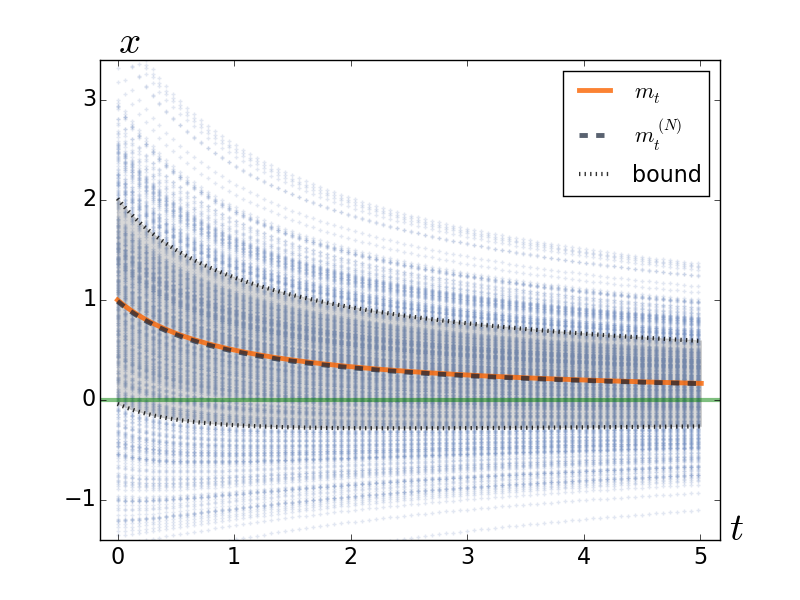
Figure 1: Simulation results with a quadratic function $h(x)=\frac{1}{2}x^{2}$. Trajectories of $N=500$ particles is depicted as dots in the background. The solid line is the mean $m_{t}$ obtained using the exact formula (21) and the dashed line is its empirical estimate obtained using the particles. The shaded region depicts the $\pm 1$ standard deviation bound.

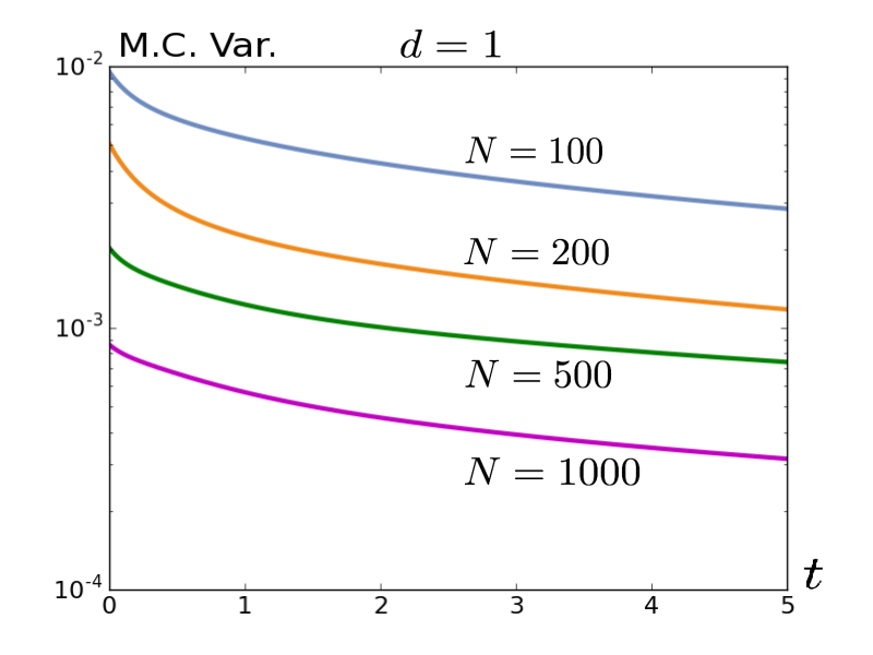
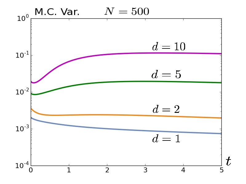
Figure 2: Comparison of the M.C. variance of the estimated mean as a function of the number of particles $N$ (part (a)) and the dimension $d$ (part (b)).

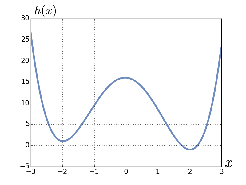
Figure 3: Double-well potential.

IV Numerical Examples

Results of numerical experiments are presented next. The purpose is to illustrate the algorithms with simple examples. A comprehensive numerical study on benchmark problems including comparisons with other algorithms will be a subject of a separate publication.

IV-A Quadratic Gaussian Case

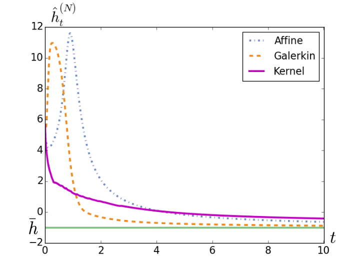
Figure 4: Comparison of $\hat{h}_{t}^{(N)}$ with the three types of approximate control laws.

Consider the quadratic function $h(x)=\frac{1}{2}\,|x|^{2}$ for $x\in\mathbb{R}^{d}$. For a quadratic function with a Gaussian prior, the optimal solution is known in closed-form (see Sec. II-B).

The simulation parameters are as follows: The simulations are carried out over a finite time-horizon $[0,T]$ with $T=5$, a fixed time step $\Delta t=0.01$, and the parameter $\beta=1$. An Euler discretization is used to numerically integrate the ode (4). At each discrete time step, the algorithm in Table 1 is used to approximate the affine control law. The filter is initialized with samples drawn i.i.d. from the Gaussian distribution ${\cal N}(m_{0},\Sigma_{0})$, where $m_{0}=(1,...,1)\in\mathbb{R}^{d}$ and $\Sigma_{0}=\text{diag}(1,...,1)$.

Figure 1 depicts a typical simulation result for $d=1$ and $N=500$. The empirical mean $m_{t}^{(N)}$ is seen to closely match its mean-field limit $m_{t}$ obtained using the exact formula (21).

Figure 2 depicts the results of Monte Carlo experiments: The part (a) is a plot of Monte Carlo (M.C.) variance for estimated mean as the number of particles $N$ is varied with $d=1$ fixed, and the part (b) is the corresponding plot as $d$ is varied with $N=500$ fixed. The M.C. variance is defined as:

$$\text{M. C. Var}(m_{t}^{(N)}) :=\frac{1}{J}\sum_{j=1}^{J}|m_{t,j}^{(N)}-\frac{1}{J}\sum_{j=1}^{J}m_{t,j}^{(N)}|^{2}$$

with $J=100$ independent runs used in the experiment.

IV-B Double-Well Potential

Consider a double-well potential $h(x)=(x-2)^{2}(x+2)^{2}-\frac{x}{2}$, as depicted in Figure 3. Figure 4 depicts a comparison of $\hat{h}_{t}^{(N)}=N^{-1}\sum_{i}h(X_{t}^{i})$ with the three types of approximate control laws: the affine approximation given in Table 1, the Galerkin approximation given in Table 2, and the kernel approximation given in Table 3. With the optimal control, Theorem 4 shows that $\hat{h}_{t}$ decreases monotonically as a function of time. This was indeed found to be the case with the kernel-based algorithm but not so with the other two. Even though the particles in all three cases eventually converge to the correct equilibrium (see Fig. 5), the approximate nature of the control can lead to a transient growth of $\hat{h}_{t}^{(N)}$.

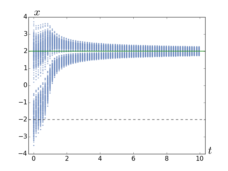
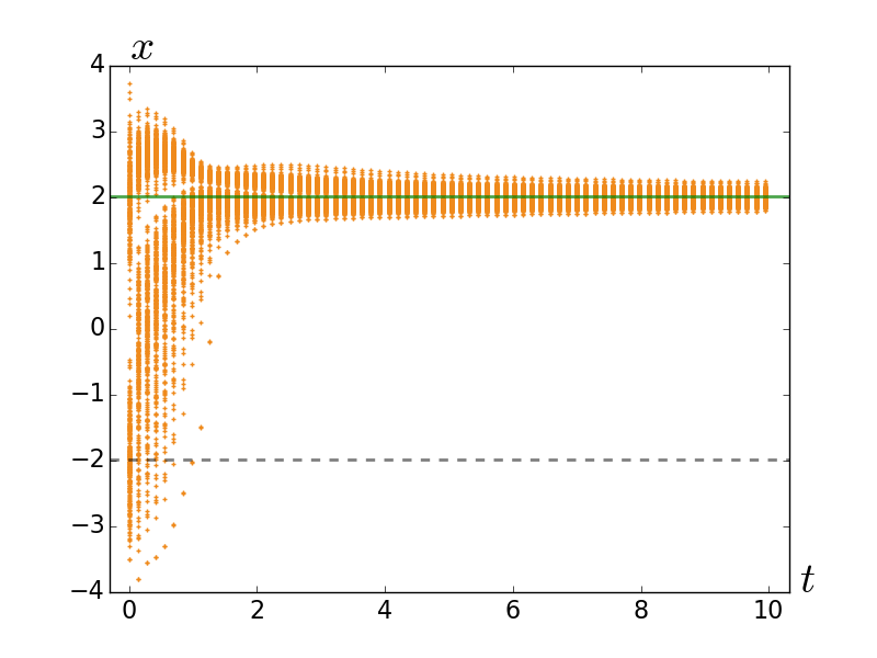
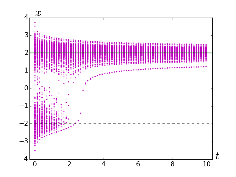
Figure 5: Particle trajectories with the three approximate control laws: (a) affine control, (b) Galerkin control, and (c) kernel-based control. The global and the local minimizers are depicted via the solid and dashed lines, respectively.

For each simulation, $N=500$ particles are used. The initial particles $X_{0}^{i}$ are sampled i.i.d. from a mixture of two Gaussians, ${\cal N}(-2,\,0.6^{2})$ and ${\cal N}(2,\,0.6^{2})$, with equal weights. An Euler discretization is used to numerically integrate the ode (4) with $\Delta t=0.01$ and $\beta=1$. For the Galerkin approximation, the basis functions are $\text{span}\Big{\{}x,~{}\cos\big{(}\frac{2\pi}{10}\,x\big{)},~{}\sin\big{(}\frac{2\pi}{10}\,x\big{)}\Big{\}}$. For the kernel approximation, the parameter $\epsilon=0.5$. The Galerkin approximation can suffer from numerical instability on account of ill-conditioning of the matrix $A$. This can lead to relatively large values of control requiring small time-steps for numerical integration.

-C Poisson’s Equation

This section includes background on the existence-uniqueness results for the Poisson equation (5). The appropriate function space for the solution is the co-dimension 1 subspace $L^{2}_{0}(\mathbb{R}^{d},\rho):=\{\phi\in L^{2}(\mathbb{R}^{d},\rho);\int\phi\rho\,\mathrm{d}x=0\}$ and $H^{1}_{0}(\mathbb{R}^{d},\rho):=\{\phi\in H^{1}(\mathbb{R}^{d},\rho);\int\phi\rho\,\mathrm{d}x=0\}$; cf. [22, 35].

A function $\phi\in H_{0}^{1}(\mathbb{R}^{d};\rho)$ is said to be a weak solution of the Poisson’s equation (5) if

$$\int\nabla\phi(x)\cdot\nabla\psi(x)\rho(x)\,\mathrm{d}x=\int(h(x)-\hat{h})\psi(x)\rho(x)\,\mathrm{d}x$$ (33)

for all $\psi\in H^{1}(\mathbb{R}^{d};\rho)$.

Theorem 5 (Theorem 2.2. in [22])

Suppose the density $\rho$ admits a spectral gap (or Poincaré inequality) ([1] Thm 4.6.3), i.e., $\exists\;\lambda_{1}>0$ such that

$$\int f(x)^{2}\,\rho(x)\,\mathrm{d}x\leq\frac{1}{\lambda_{1}}\int|\nabla f(x)|^{2}\,\rho(x)\,\mathrm{d}x,\quad\forall f\in H^{1}_{0}(\mathbb{R}^{d},\rho).$$ (34)

Then for each $h\in L^{2}(\mathbb{R}^{d};\rho)$, there exists a unique weak solution $\phi\in H_{0}^{1}(\mathbb{R}^{d};\rho)$ satisfying (33). Moreover, the derivative of the solution is controlled by the size of the data:

$$\int|\nabla\phi(x)|^{2}\rho(x)\,\mathrm{d}x\leq\frac{1}{\lambda_{1}}\int|h(x)-\hat{h}|^{2}\rho(x)\,\mathrm{d}x.$$ (35)

∎

An alternate but equivalent approach to obtain the solution of (5) is to first note that the weighted Laplacian $\Delta_{\rho}:=\frac{1}{\rho}\nabla\cdot(\rho\nabla)$ is the infinitesimal generator of a Markov semigroup, denoted in this paper as $e^{\epsilon\Delta_{\rho}}$; cf., [1]. In terms of this semigroup, the Poisson’s equation (5) is equivalently expressed as, for fixed $\epsilon>0$,

$$\phi=e^{\epsilon\Delta_{\rho}}\phi+\int_{0}^{\epsilon}e^{s\Delta_{\rho}}(h-\hat{h})\,\mathrm{d}s.$$ (36)

If the density $\rho$ admits a spectral gap (i.e., (34) holds for some $\lambda_{1}>0$) then $e^{\epsilon\Delta_{\rho}}$ is a contraction on $L^{2}_{0}(\mathbb{R}^{d},\rho)$ and a unique solution exists by the contracting mapping theorem.

The two formulations for obtaining the solution, viz., (33) and (36), inform the two algorithms for numerically approximating the control law. These algorithms are presented in Sec. III-A and Sec. III-B, respectively.

-D Gradient flow

Proof of Theorem 8: As $\Delta t_{n}\downarrow 0$, $\rho^{(\bar{N})}(x,t)\rightarrow p^{*}(x,t)$, the posterior density defined in (1). By direct substitution, it is verified that $p^{*}$ is a solution of the replicator pde (8).

In the conference version of this paper (see [40]), the replicator pde is derived based on variational analysis. The main steps of the variational proof are as follows:

• By taking the first variation of the functional (7), the minimizer $\rho_{n}$ is shown to satisfy the E-L equation:

  $$\int\frac{\rho_{n}}{\rho_{n-1}}\nabla\cdot(\rho_{n-1}\,\varsigma)\,\mathrm{d}x-\Delta t_{n}\;\beta\int\nabla h\cdot\varsigma\rho_{n}\,\mathrm{d}x=0,$$ (37)

  for each vector field $\varsigma\in L^{2}(\mathbb{R}^{d};\rho_{n-1})$.

• Given any $C^{1}$ smooth and compactly supported (test) function $f$, let $\xi_{n}\in L^{2}(\mathbb{R}^{d};\rho_{n-1})$ be the solution of

  $$\nabla\cdot(\rho_{n-1}\xi_{n})=(f-\hat{f}_{n-1})\rho_{n-1},$$ (38)

  where $\hat{f}_{n-1}:=\int f\rho_{n-1}\,\mathrm{d}x$. Then, using the E-L equation (37),

  $$\hat{f}_{n}-\hat{f}_{n-1}=\Delta t_{n}\;\beta\int\nabla h\cdot\xi_{n}\rho_{n}\,\mathrm{d}x,$$

  and upon summing,

  $$\hat{f}_{\bar{N}}=\hat{f}_{0}+\beta\sum_{n=1}^{\bar{N}}\Delta t_{n}\int\nabla h\cdot\xi_{n}\rho_{n}\,\mathrm{d}x.$$ (39)

• Integrating by parts and using (38),

  $$\int\nabla h\cdot\xi_{n}\rho_{n}\,\mathrm{d}x=-\int h(f-\hat{f}_{n-1})\rho_{n-1}\,\mathrm{d}x+{\cal E}_{n},$$

  where the error term ${\cal E}_{n}=O(\Delta t_{n})$. Equation (39) thus becomes

  $$\hat{f}_{\bar{N}}=\hat{f}_{0}-\beta\sum_{n=1}^{\bar{N}}\Delta t_{n}\int h(f-\hat{f}_{n-1})\rho_{n-1}\,\mathrm{d}x+\sum_{n=1}^{\bar{N}}\Delta t_{n}\mathcal{E}_{n}.$$

• On taking the limit as $\Delta t_{n}\downarrow 0$, the limiting density $p^{*}(x,t)$ satisfies

  $$\hat{f}_{t} =\hat{f}_{0}-\beta\int_{0}^{t}\int h(x)(f(x)-\hat{f}_{s})p^{*}(x,s)\,\mathrm{d}x\,\mathrm{d}s$$

  $$=\hat{f}_{0}-\beta\int_{0}^{t}\int(h(x)-\hat{h}_{s})f(x)p^{*}(x,s)\,\mathrm{d}x\,\mathrm{d}s$$

  for all test functions $f$, showing that $p^{*}(x,t)$ is a weak solution of the replicator pde (1). For additional details on these calculations, see [40].

-E Optimal control

Preliminaries: Consider a functional $E:{\cal P}\to\mathbb{R}$ mapping densities to real numbers. For a fixed $\rho\in{\cal P}$, the (Gâteaux) derivative of $E$ is a real-valued function on $\mathbb{R}^{d}$, and an element of the function space $L^{2}(\mathbb{R}^{d};\rho)$. This function is denoted as $\frac{\partial E}{\partial\rho}(\rho,t)(x)$ for $x\in\mathbb{R}^{d}$, and defined as follows:

$$\frac{\,\mathrm{d}}{\,\mathrm{d}t}E(\rho_{t})\bigg{|}_{t=0}=-\int_{\mathbb{R}^{d}}\frac{\partial E}{\partial\rho}(\rho)(x)\nabla\cdot(\rho(x)u(x))\,\mathrm{d}x,$$

where $\rho_{t}$ is a path in ${\cal P}$ such that $\frac{\partial\rho_{t}}{\partial t}=-\nabla\cdot(\rho_{t}u)$ with $\rho_{0}=\rho$, and $u$ is any arbitrary vector-field on $\mathbb{R}^{d}$. Similarly, $\frac{\partial^{2}E}{\partial\rho^{2}}(\rho)\in L^{2}(\mathbb{R}^{d}\times\mathbb{R}^{d})$ is the second (Gâteaux) derivative of the functional $E$ if

$$\frac{\,\mathrm{d}}{\,\mathrm{d}t}\frac{\partial E}{\partial\rho}(\rho_{t})(x)\bigg{|}_{t=0}=-\int_{\mathbb{R}^{d}}\frac{\partial^{2}E}{\partial\rho^{2}}(\rho)(x,y)\nabla\cdot(\rho(y)u(y))\,\mathrm{d}y.$$

The optimal control problems (10) and (14) are examples of the mean-field type control problem introduced in [2]. The notation and the methodology for the following proofs is based in part on [2].

Proof of Theorem 2: The value function $V(\rho,t)$, defined in (12), is the solution of the DP equation:

$$\frac{\partial V}{\partial t}(\rho,t) +\inf_{u\in L^{2}}~{}{\sf H}(\rho,\frac{\partial V}{\partial\rho}(\rho,t),u)=0,\quad t\in[0,T),$$ (40)

$$V(\rho,T) =\beta\int h(x)\rho(x)\,\mathrm{d}x.$$

In the following, we use the notation

$$\Theta=\Theta(\rho,t)(x):=\frac{\partial V}{\partial\rho}(\rho,t)(x).$$

For a fixed $\rho\in{\cal P}$ and $t\in[0,T)$, $\Theta$ is a function on $\mathbb{R}^{d}$.

A necessary condition is obtained by considering the first variation of ${\sf H}$. Suppose $u$ is a minimizing control function. Then $u$ satisfies the first order optimality condition:

$$\left.\frac{\,\mathrm{d}}{\,\mathrm{d}\epsilon}{\sf H}(\rho,\Theta,u+\epsilon v)\right|_{\epsilon=0}=0,$$

where $v$ is an arbitrary vector field on $\mathbb{R}^{d}$. Explicitly,

$$\int\nabla(-\frac{1}{\rho}\nabla\cdot(\rho u)+\Theta)\cdot v\;\rho\,\mathrm{d}x=0,$$

or in its strong form

$$-\frac{1}{\rho}\nabla\cdot(\rho u)+\Theta=(\text{constant}).$$

Multiplying both sides by $\rho$ and integrating yields the value of the constant as $\int\Theta(\rho,t)(x)\rho(x)\,\mathrm{d}x=:\hat{\Theta}(\rho,t)$. Therefore, the minimizing control solves the pde

$$\frac{1}{\rho}\nabla\cdot(\rho u)=\Theta-\hat{\Theta}.$$

On substituting the optimal control law into the DP equation (40), the HJB equation for the value function is given by

$$\frac{\partial V}{\partial t}(\rho,t) +\frac{\beta^{2}}{2}\int|h-\hat{h}|^{2}\rho\,\mathrm{d}x$$

$$-\frac{1}{2}\int(\Theta(\rho,t)-\hat{\Theta}(\rho,t))^{2}\rho\,\mathrm{d}x=0,\quad t\in[0,T),$$

$$V(\rho,T) =\beta\int h(x)\rho(x)\,\mathrm{d}x.$$

The equation involves both $V$ and $\Theta$. One obtains the so-called master equation (see [2]) involving only $\Theta$ by differentiating with respect to $\rho$

$$\frac{\partial\Theta}{\partial t}(\rho,t)(x)+\frac{\beta^{2}}{2}|h(x)-\hat{h}|^{2}-\frac{1}{2}|\Theta(\rho,t)(x)-\hat{\Theta}(\rho,t)|^{2}$$

$$-\int(\Theta(\rho,t)(y)-\hat{\Theta}(\rho,t))\frac{\partial\Theta}{\partial\rho}(\rho,t)(y,x)\rho(y)\,\mathrm{d}y=0,\;t\in[0,T),$$

$$\Theta(\rho,T)=\beta h.$$

It is easily verified that $\Theta(\rho,t)=\beta h$ solves the master equation. The corresponding value function $V(\rho,t)=\beta\int h\rho\,\mathrm{d}x$.

Sufficiency: The proof that the proposed control law is a minimizer is as follows. Consider any arbitrary control law $v_{t}$ with the resulting density $\rho_{t}$. Taking the time derivative of $-\beta\int h\rho_{t}\,\mathrm{d}x$:

$$-\beta\frac{\,\mathrm{d}}{\,\mathrm{d}t}\int h\rho_{t}\,\mathrm{d}x =\beta\int h\;\nabla\cdot(\rho_{t}v_{t})\,\mathrm{d}x$$

$$=\int\beta(h-\hat{h}_{t})\;(\frac{1}{\rho_{t}}\nabla\cdot(\rho_{t}v_{t}))\;\rho_{t}\,\mathrm{d}x$$

$$\leq\int\left(\frac{\beta^{2}}{2}(h-\hat{h})^{2}+\frac{1}{2}\left|\frac{1}{\rho_{t}}\nabla\cdot(\rho_{t}v_{t})\right|^{2}\right)\rho_{t}\,\mathrm{d}x$$

$$={\sf L}(\rho_{t},v_{t}).$$

On integrating both sides with respect to time,

$$\beta\int_{\mathbb{R}^{d}}h\rho_{0}\,\mathrm{d}x \;\leq\;\int_{0}^{T}{\sf L}(\rho_{t},v_{t})\,\mathrm{d}t\;+\;\beta\int_{\mathbb{R}^{d}}h\rho_{T}\,\mathrm{d}x,$$

where the equality holds with $v_{t}=u_{t}$ (defined as solution of (13)). Therefore,

$$J(u)=\beta\int h\rho_{0}\,\mathrm{d}x\leq J(v).$$

This also confirms that $V(\rho,t)=\beta\int h\rho\,\mathrm{d}x$ is the value function, and completes the proof of Theorem 2.  ∎

The analysis for the infinite horizon optimal control problem (14) is similar and described next.

Proof of Theorem 3: The infinite-horizon value function $V^{\infty}(\rho):=\mathop{\inf}_{u}\int_{0}^{\infty}{\sf L}(\rho_{t},u_{t})\,\mathrm{d}t$ is a solution of the DP equation:

$$\inf_{u\in L^{2}}~{}{\sf H}(\rho,\Theta^{\infty}(\rho),u)=0,$$ (41)

where $\Theta^{\infty}(\rho):=\frac{\partial V^{\infty}}{\partial\rho}(\rho)$. By carrying out the first order analysis in an identical manner, it is readily verified that:

• A minimizing control $u$ is a solution of the pde (13);

• $V^{\infty}(\rho)=\beta\int h\rho\,\mathrm{d}x-\beta h(\bar{x})$ is a solution of the DP equation (41).

The sufficiency also follows similarly. With any arbitrary control $v_{t}$,

$$\beta\int_{\mathbb{R}^{d}}h\rho_{0}\,\mathrm{d}x\leq\int_{0}^{\infty}{\sf L}(\rho_{t},v_{t})\,\mathrm{d}t+\beta\limsup_{t\to\infty}\int_{\mathbb{R}^{d}}h\rho_{t}\,\mathrm{d}x,$$

with equality if $v_{t}=u_{t}$ solves the pde (13). Using the boundary condition, $\limsup_{t\to\infty}\int h\rho_{t}\,\mathrm{d}x=h(\bar{x})$,

$$J(u)=\beta\int h\rho_{0}\,\mathrm{d}x-\beta h(\bar{x})\leq J(v).$$

∎

Proof of Lemma 1: Suppose $\phi$ is the unique solution of the Poisson equation (5) (Theorem 5 in Appendix -C). Then $u=-\beta\nabla\phi$ is a particular solution of the pde (13). The general solution is then given by $u=v-\beta\nabla\phi$ where $v$ is a null solution, i.e., $\nabla\cdot(\rho v)=0$. The $L^{2}$ optimality of the gradient solution follows from the simple calculation:

$$\int|u|^{2}\rho\,\mathrm{d}x =\int\beta^{2}|\nabla\phi|^{2}\rho\,\mathrm{d}x+\int|v|^{2}\rho\,\mathrm{d}x-2\beta\int v\cdot\nabla\phi\rho\,\mathrm{d}x$$

$$=\beta^{2}\|\nabla\phi\|_{2}^{2}+\|v\|^{2}_{2},$$

because $\int\nabla\phi\cdot v\rho\,\mathrm{d}x=-\int\phi\nabla\cdot(\rho v)\,\mathrm{d}x=0$.  ∎

-F Hamiltonian formulation

The Hamiltonian ${\sf H}$ is defined in (11). Suppose $u_{t}$ is the optimal control and $\rho_{t}$ is the corresponding optimal trajectory. Denote the trajectory for the co-state (momentum) as ${\sf q}_{t}$. Using the Pontryagin’s minimum principle, $(\rho_{t},{\sf q}_{t})$ satisfy the following Hamilton’s equations:

$$\frac{\partial\rho_{t}}{\partial t} =\frac{\partial{\sf H}}{\partial\rho}(\rho_{t},{\sf q}_{t},u_{t}),\quad\rho_{0}=p^{*}_{0},$$

$$\frac{\partial{\sf q}_{t}}{\partial t} =-\frac{\partial{\sf H}}{\partial{\sf q}}(\rho_{t},{\sf q}_{t},u_{t}),\quad{\sf q}_{T}=\frac{\partial}{\partial\rho}\left(\beta\int h(x)\rho(x)\,\mathrm{d}x\right),$$

$$0 ={\sf H}(\rho_{t},{\sf q}_{t},u_{t})=\min_{v\in L^{2}}{\sf H}(\rho_{t},{\sf q}_{t},v).$$

The calculus of variation argument in the proof of Theorem 2 shows that the minimizing control $u_{t}$ solves the first order optimality equation

$$\frac{1}{\rho_{t}}\nabla\cdot(\rho_{t}u_{t})={\sf q}_{t}-\hat{\sf q}_{t},$$ (42)

where $\hat{\sf q}_{t}:=\int{\sf q}_{t}(x)\rho_{t}(x)\,\mathrm{d}x$.

The explicit form of the Hamilton’s equations are obtained by explicitly evaluating the derivatives along the optimal trajectory:

$$\frac{\partial{\sf H}}{\partial\rho}(\rho_{t},{\sf q}_{t},u_{t}) =-\nabla\cdot(\rho_{t}u_{t}),$$

$$\frac{\partial{\sf H}}{\partial{\sf q}}(\rho_{t},{\sf q}_{t},u_{t}) =\frac{\beta^{2}}{2}(h-\hat{h}_{t})^{2}-\frac{1}{2}({\sf q}_{t}-\hat{\sf q}_{t})^{2}.$$

It is easy to verify that ${\sf q}_{t}\equiv{\beta}h(x)$ satisfies both the boundary condition and the evolution equation for the momentum. This results in a simpler form of the Hamilton’s equations:

$$\frac{\partial\rho_{t}}{\partial t} =-\nabla\cdot(\rho_{t}u_{t}),$$

$$0 ={\sf H}(\rho_{t},{\scriptstyle\beta}h,u_{t})=\min_{v\in L^{2}}{\sf H}(\rho_{t},{\scriptstyle\beta}h,v).$$

In a particle filter implementation, the minimizing control $u_{t}=-\nabla\phi$ is obtained by solving the first order optimality equation (42) with ${\sf q}_{t}=\beta h$.

-G Bayes’ exactness and convergence

Before proving the Theorem 4, we state and prove the following technical Lemma:

Lemma 3

Suppose the prior density $p_{0}^{*}(x)$ satisfies Assumption (A1) and the objective function $h(x)$ satisfies assumption (A2). Then for each fixed time $t\geq 0$:

• The posterior density $p^{*}(x,t)$, defined according to (1), admits a spectral bound;

• The objective function $h\in L^{2}(\mathbb{R}^{d};p^{*}(\cdot,t))$.

Proof 1

Define $V_{t}(x):=-\log p^{*}(x,t)=V_{0}(x)+t\beta h(x)+\gamma_{t}$ where $\gamma_{t}:=\log(\int e^{-V_{0}(y)-th(y)}\,\mathrm{d}y)$. It is directly verified that $V_{t}\in C^{2}$ with $D^{2}V_{t}\in L^{\infty}$ and $\liminf_{|x|\to\infty}\;\;\nabla V_{t}(x)\cdot\frac{x}{|x|}=\infty$. Therefore, the density $p^{*}(x,t)$ admits a spectral bound [Thm 4.6.3 in [1]]. The function $h$ is square-integrable because

$$\int|h(x)|^{2}p^{*}(x,t)\,\mathrm{d}x\leq e^{-\beta t\bar{h}-\gamma_{t}}\int|h(x)|^{2}e^{-V_{0}(x)}\,\mathrm{d}x<\infty.$$

∎

Proof of Theorem 4: Given any $C^{1}$ smooth and compactly supported (test) function $f$, using the elementary chain rule,

$$\,\mathrm{d}f(X_{t}^{i})=-\beta\nabla\phi(X_{t}^{i})\cdot\nabla f(X_{t}^{i}).$$

On integrating and taking expectations,

$${\sf E}[f(X_{t}^{i})] ={\sf E}[f(X_{0}^{i})]-\beta\int_{0}^{t}{\sf E}[\nabla\phi(X_{s}^{i})\cdot\nabla f(X_{s}^{i})]\,\mathrm{d}s$$

$$={\sf E}[f(X_{0}^{i})]-\beta\int_{0}^{t}{\sf E}[(h(X_{s}^{i})-\hat{h}_{s})f(X_{s}^{i})]\,\mathrm{d}s,$$

which is the weak form of the replicator pde (8). Note that the weak form of the Poisson equation (33) is used to obtain the second equality. Since the test function $f$ is arbitrary, the evolution of $p$ and $p^{*}$ are identical. That the control function is well-defined for each time follows from Theorem 5 based on apriori estimates in Lemma 3 for $p^{*}=p$.

The convergence proof is presented next. The proof here is somewhat more general than needed to prove the Theorem. For a function $h$, we define the minimizing set:

$$A_{0}:=\{x\in\mathbb{R}^{d}\mid h(x)=\bar{h}\},$$

where it is recalled that $\bar{h}=\inf_{x\in\mathbb{R}^{d}}h(x)$. In the following it is shown that for any open neighborhood $U$ of $A_{0}$,

$$\liminf_{t\to\infty}\int_{U}p(x,t)\,\mathrm{d}x=1.$$ (43)

It then follows that $X_{t}^{i}$ converges in distribution where the limiting distribution is supported on $A_{0}$ [Thm. 3.2.5 in [10]]. If the minimizer is unique (i.e., $A_{0}=\{\bar{x}\}$), $X^{i}_{t}$ converges to $\bar{x}$ in probability.

The key to prove the convergence is the following property of the function $h$:

(P1): For each $\delta>0$, $\exists\;\epsilon>0$ such that:

$$|h(x)-\bar{h}|\leq\epsilon\quad\Rightarrow\quad\text{dist}(x,A_{0})\leq\delta\quad\forall x\in\mathbb{R}^{d},$$

where $\text{dist}(x,A_{0})$ denotes the Euclidean distance of point $x$ from set $A_{0}$. If the minimizer $\bar{x}$ is unique, it equals $|x-\bar{x}|$.

Any lower semi-continuous function satisfying Assumption (A3) also satisfies the property (P1): Suppose $\{x_{n}\}$ is a sequence such that $h(x_{n})\rightarrow\bar{h}$. Then $\{x_{n}\}$ is compact because $h(x)>\bar{h}+r$ outside some compact set. Therefore, the limit set is non-empty and because $h$ is lower semi-continuous, for any limit point $z$, $\bar{h}\leq h(z)\leq\liminf_{x_{n}\rightarrow z}h(x_{n})=\bar{h}$. That is, $z\in A_{0}$.

The proof for (43) is based on construction of a Lyapunov function: Denote $A_{\epsilon}:=\{x\in\mathbb{R}^{d}\mid h(x)\leq\bar{h}+\epsilon\}$ where $\epsilon>0$. By property (P1), given any open neighborhood $U$ containing $A_{0}$, $\exists\;\epsilon>0$ such that $A_{\epsilon}\subset U$. A candidate Lyapunov function $V_{A_{\epsilon}}(\mu):=-\beta^{-1}\log(\mu(A_{\epsilon}))$ is defined for measure $\mu$ with everywhere positive density. By construction $V_{A_{\epsilon}}(\mu)\geq 0$ with equality iff $\mu(A_{\epsilon})=1$.

Let $\mu_{t}$ be the probability measure associated with $p(x,t)$, i.e, $\mu_{t}(B):=\int_{B}p(x,t)\,\mathrm{d}x$ for all Borel measurable set $B\subset\mathbb{R}^{d}$. Since $p(x,t)$ is a solution of the replicator pde,

$$\frac{\,\mathrm{d}}{\,\mathrm{d}t}V_{A_{\epsilon}}(\mu_{t}) =\frac{\,\mathrm{d}}{\,\mathrm{d}t}\big{[}-\frac{1}{\beta}\log(\mu_{t}(A_{\epsilon}))\big{]}$$

$$=\frac{1}{\mu_{t}(A_{\epsilon})}\int_{A_{\epsilon}}(h(x)-\hat{h}_{t})\,\mathrm{d}\mu_{t}(x)$$

$$=(1-\mu_{t}(A_{\epsilon}))\left(\frac{\int_{A_{\epsilon}}h\,\mathrm{d}\mu_{t}}{\mu_{t}(A_{\epsilon})}-\frac{\int_{A_{\epsilon}^{c}}h\,\mathrm{d}\mu_{t}}{\mu_{t}(A_{\epsilon}^{c})}\right)$$

$$\leq 0$$

with equality iff $\mu_{t}(A_{\epsilon})=1$.

For the objective function $h$, a direct calculation also shows:

$$\frac{\,\mathrm{d}}{\,\mathrm{d}t}\int h(x)p(x,t)\,\mathrm{d}x =-\beta\int h(x)(h(x)-\hat{h}_{t})p(x,t)\,\mathrm{d}x$$

$$=-\beta\int(h(x)-\hat{h})^{2}p(x,t)\,\mathrm{d}x\leq 0,$$

with equality iff $h=\hat{h}$ almost everywhere (with respect to the measure $\mu_{t}$).  ∎

-H Quadratic Gaussian case

Proof of Lemma 2: We are interested in obtaining an explicit solution of the Poisson equation,

$$-\nabla\cdot(\rho(x)\nabla\phi(x))=(h(x)-\hat{h})\rho(x).$$ (44)

Consider the solution ansatz:

$$\nabla\phi(x)={\sf K}(x-m)+b,$$ (45)

where the matrix ${\sf K}={\sf K}^{T}\in\mathbb{R}^{d\times d}$ and the vector $b\in\mathbb{R}^{d}$ are determined as follows:

• Multiply both sides of (44) by vector $x$ and integrate (element-by-element) by parts to obtain

  $$b=\int x(h(x)-\hat{h})\rho(x)\,\mathrm{d}x.$$ (46)

• Multiply both sides of (44) by matrix $(x-m)(x-m)^{T}$ and integrate by parts to obtain

  $$\Sigma{\sf K}+{\sf K}\Sigma=\int(x-m)(x-m)^{T}(h(x)-\hat{h})\rho(x)\,\mathrm{d}x.$$ (47)

We have thusfar not used the fact that the density $\rho$ is Gaussian and the function $h$ is quadratic. In the following, it is shown that the solution thus defined in fact solves the pde (44) under these conditions.

A radially unbounded quadratic function is of the general form:

$$h(x)=\frac{1}{2}(x-\bar{x})^{T}H(x-\bar{x})+c$$

where the matrix $H=H^{T}\succ 0$ and $c$ is some constant. For a Gaussian density $\rho$ with mean $m$ and variance $\Sigma\succ 0$, the integrals are explicitly evaluated to obtain

$$b =\int x(h(x)-\hat{h})\rho(x)\,\mathrm{d}x=\Sigma H(m-\bar{x}),$$ (48a)

$$\Sigma{\sf K}+{\sf K}\Sigma =\int(x-m)(x-m)^{T}(h(x)-\hat{h})\rho(x)\,\mathrm{d}x=\Sigma H\Sigma.$$ (48b)

A unique positive-definite symmetric solution ${\sf K}$ exists for the Lyapunov equation (48b) because $\Sigma\succ 0$ and $\Sigma H\Sigma\succ 0$ [9].

On substituting the solution (45) into the Poisson equation (44) and dividing through by $\rho$, the two sides are:

$$-\frac{1}{\rho}\nabla\cdot(\rho\nabla\phi)=(x-m)^{T}\Sigma^{-1}({\sf K}(x-m)+b)-\mbox{tr}({\sf K}),$$

$$h-\hat{h}=\frac{1}{2}(x-\bar{x})^{T}H(x-\bar{x})-\frac{1}{2}(m-\bar{x})^{T}H(m-\bar{x})-\frac{1}{2}\mbox{tr}(H\Sigma).$$

where $\mbox{tr}(\cdot)$ denotes the matrix trace. Using formulae (48a)-(48b) for $b$ and ${\sf K}$, the two sides are seen to be equal.  ∎

Proof of Proposition 1: Using the affine control law (16), the particle filter is a linear system with a Gaussian prior:

$$\frac{\,\mathrm{d}X^{i}_{t}}{\,\mathrm{d}t}=-\beta{\sf K}_{t}(X^{i}_{t}-m_{t})-\beta b_{t},\quad X^{i}_{0}\sim{\cal N}(m_{0},\Sigma_{0}).$$ (49)

Therefore, the density of $X_{t}^{i}$ is Gaussian for all $t>0$. The evolution of the mean is obtained by taking an expectation of both sides of the ode (49):

$$\frac{\,\mathrm{d}}{\,\mathrm{d}t}{\sf E}[X^{i}_{t}]=-\beta b_{t}=-\beta{\sf E}[X_{t}^{i}(h(X_{t}^{i})-\hat{h}_{t})],$$

where (17) is used to obtain the second equality. The equation for the variance $\Sigma_{t}$ of $X_{t}^{i}$ is similarly obtained:

$$\frac{\,\mathrm{d}\Sigma_{t}}{\,\mathrm{d}t} =-\beta({\sf K}_{t}\Sigma_{t}+\Sigma_{t}{\sf K}_{t})$$

$$=-\beta{\sf E}\left[(X_{t}^{i}-m_{t})(X_{t}^{i}-m_{t})^{T}(h(X_{t}^{i})-\hat{h}_{t})\right],$$

where (18) has been used. ∎

Proof of Corollary 1: The closed-form odes (20a) and (20b) are obtained by using explicit formulae (48a) and (48b) for $b$ and ${\sf K}$, respectively.  ∎

-I Parametric case

Proof of Theorem 26: The natural gradient ode (26) is obtained by applying the chain rule. In its parameterized form, the density $p(x,t)=\Varrho(x;\theta_{t})$ evolves according to the replicator pde:

$$\frac{\partial\Varrho}{\partial t}(x;\theta_{t})=-\beta\,(h(x)-\hat{h}_{t})\,\Varrho(x;\theta_{t}).$$

Now, using the chain rule,

$$\frac{\partial\Varrho}{\partial t}(x,\theta_{t})=\Varrho(x,\theta_{t})\left[\frac{\partial}{\partial\vartheta}(\log\Varrho(x;\theta_{t}))\right]^{T}\frac{\,\mathrm{d}\theta_{t}}{\,\mathrm{d}t},$$

where $\frac{\partial}{\partial\vartheta}\left(\log\Varrho\right)$ and $\frac{\,\mathrm{d}\theta_{t}}{\,\mathrm{d}t}$ are both $M\times 1$ column vectors. Therefore, the replicator pde is given by

$$\left[\frac{\partial}{\partial\vartheta}(\log\Varrho(x;\theta_{t}))\right]^{T}\frac{\,\mathrm{d}\theta_{t}}{\,\mathrm{d}t}\Varrho(x;\theta_{t})=-\beta(h(x)-\hat{h}_{t})\Varrho(x;\theta_{t}).$$

Multiplying both sides by the column vector $\frac{\partial}{\partial\vartheta}\left(\log\Varrho\right)$, integrating over the domain, and using the definitions (24) of the Fisher information matrix $G$ and (25) for $\nabla e$, one obtains

$$G_{(\theta_{t})}\frac{\,\mathrm{d}\theta_{t}}{\,\mathrm{d}t}=-\beta\nabla e(\theta_{t}).$$

The ode (26) is obtained because $G$ is assumed invertible.  ∎

-J Galerkin approximation error

Spectral representation: Under Assumptions (A1)-(A2), the spectrum of $-\Delta_{\rho}$ is known to be discrete with an ordered sequence of eigenvalues $0=\lambda_{0}<\lambda_{1}\leq\lambda_{2}\leq\ldots$ and associated eigenfunctions $\{e_{n}\}$ that form a complete orthonormal basis of $L^{2}(\mathbb{R}^{d},\rho)$ [Corollary 4.10.9 in  [1]]. As a result, for $m,l\in\mathbb{Z}^{+}$:

$$\big{<}e_{k},e_{l}\big{>}=\delta_{kl},\quad\big{<}\nabla e_{k},\nabla e_{l}\big{>}=\lambda_{m}\delta_{kl}.$$

The trivial eigenvalue $\lambda_{0}=0$ with associated eigenfunction $e_{0}(x)=1$. On the subspace of zero-mean functions, the spectral representation yields: For $\phi\in L^{2}_{0}(\mathbb{R}^{d},\rho)$,

$$-\Delta_{\rho}\phi(x)=\sum_{k=1}^{\infty}\lambda_{k}\big{<}e_{k},\phi\big{>}e_{k}(x).$$ (50)

Proof of Proposition 3: By the triangle inequality,

$$\|\nabla\phi-\nabla\phi^{(M,N)}\|_{2}\;\leq\;\underbrace{\|\nabla\phi-\nabla\phi^{(M)}\|_{2}}_{\text{bias}}\;+\;\|\nabla\phi^{(M)}-\nabla\phi^{(M,N)}\|_{2}.$$

The estimates for the bias and for the error due to the empirical approximation are as follows:

Bias: Using the spectral representation (50), because $h-\hat{h}\in L^{2}_{0}$,

$$\phi(x)=-\Delta_{\rho}^{-1}(h-\hat{h})(x)=\sum_{k=1}^{\infty}\frac{1}{\lambda_{k}}\big{<}e_{k},h\big{>}e_{k}(x).$$

With basis functions as eigenfunctions,

$$\phi^{(M)}(x)=\sum_{k=1}^{M}\frac{1}{\lambda_{k}}\big{<}e_{k},h\big{>}e_{k}(x).$$

Therefore,

$$\|\nabla\phi-\nabla\phi^{(M)}\|^{2}_{2} =\sum_{k=M+1}^{\infty}\frac{1}{\lambda_{k}^{2}}|\big{<}e_{k},h\big{>}|^{2}\|\nabla e_{k}\|_{2}^{2}$$

$$=\sum_{k=M+1}^{\infty}\frac{1}{\lambda_{k}^{2}}|\big{<}e_{k},h\big{>}|^{2}\lambda_{k}\;\leq\;\frac{1}{\lambda_{M}}\|h-\Pi_{S}h\|^{2}_{2},$$

where $\Pi_{S}h(x):=\sum_{k=1}^{M}\big{<}e_{k},h\big{>}e_{k}(x)$ denotes the projection of $h$ onto $S$.

Empirical error: Suppose $\{X^{i}\}_{i=1}^{N}$ are drawn i.i.d. from the density $\rho$. The empirical solution is obtained as:

$$\phi^{(M,N)}(x)=\sum_{k=1}^{M}\frac{1}{\lambda_{k}}\left(\frac{1}{N}\sum_{i=1}^{N}e_{k}(X^{i})h(X^{i})\right)e_{k}(x),$$

and the error,

$$\phi^{(M,N)}(x)-\phi^{(M)}(x)=\sum_{k=1}^{M}\frac{1}{\lambda_{k}}z_{k}^{(N)}e_{k}(x),$$

where $z_{k}^{(N)}:=\frac{1}{N}\sum_{i=1}^{N}e_{k}(X^{i})h(X^{i})-\big{<}e_{k},h\big{>}$. Therefore,

$$\|\nabla\phi^{(M,N)}-\nabla\phi^{(M)}\|_{2}^{2}=\sum_{k=1}^{M}\frac{1}{\lambda_{k}}|z_{k}^{(N)}|^{2}=:\epsilon_{N},$$ (51)

where $\big{<}\nabla e_{k},\nabla e_{l}\big{>}=\lambda_{k}\delta_{kl}$ is used to simplify the cross-terms. Finally, by applying the Law of Large Numbers (LLN) for the random variable $z_{k}^{(N)}$, $\epsilon_{N}\stackrel{{\scriptstyle\text{a.s.}}}{{\rightarrow}}0$ as $N\rightarrow\infty$. The LLN applies because

$${\sf E}[|z_{k}^{(N)}|]\leq 2\,{\sf E}[|e_{k}(X)h(X)|]\leq 2\,\|h\|_{2}<\infty.$$

Variance: Under additional restrictions on $h$, one can obtain sharper estimates. For example, taking the expectation of both sides of (51),

$${\sf E}[\|\nabla\phi^{(M)}-\nabla\phi^{(M,N)}\|_{2}^{2}]=\sum_{k=1}^{M}\frac{{\sf E}[|z_{k}^{(N)}|^{2}]}{\lambda_{k}}.$$

Now, ${\sf E}[|z_{k}^{(N)}|^{2}]=\frac{\text{Var}(e_{k}(X^{i})h(X^{i}))}{N}$. Therefore, supposing $h\in L^{\infty}$,

$${\sf E}[\|\phi^{(M)}-\phi^{(M,N)}\|_{2}^{2}]\leq\frac{\|h\|_{\infty}^{2}}{N}{\sum_{k=1}^{M}\frac{1}{\lambda_{k}}},$$

because $\text{Var}(e_{k}(X^{i}))=1$.

In summary, for bounded functions $h$,

$${\sf E}[\|\nabla\phi-\nabla\phi^{(M,N)}\|_{2}]\;\leq\;\underbrace{\frac{\|h-\Pi_{S}h\|_{2}}{\sqrt{\lambda_{M}}}}_{\text{bias}}\;+\;\underbrace{\frac{\|h\|_{\infty}}{\sqrt{N}}\sqrt{\sum_{k=1}^{M}\frac{1}{\lambda_{k}}}}_{\text{variance}}.$$

∎

References

• [1] D. Bakry, I. Gentil, and M. Ledoux. Analysis and Geometry of Markov Diffusion Operators, volume 348. Springer Science & Business Media, 2013.
• [2] A. Bensoussan, J. Frehse, and S. C. P. Yam. The master equation in mean field theory. Journal de Mathématiques Pures et Appliquées, 103(6):1441–1474, 2015.
• [3] R. Brockett. Optimal control of the Liouville equation. AMS IP Studies in Advanced Mathematics, 39:23, 2007.
• [4] Y. Chen, T. Georgiou, and M. Pavon. On the relation between optimal transport and Schródinger bridges: A stochastic control viewpoint. J. Optimiz. Theory App., 169(2):671–691, 2016.
• [5] Y. Chen, T. Georgiou, and M. Pavon. Optimal steering of a linear stochastic system to a final probability distribution, part I. IEEE Trans. Autom. Control, 61(5):1158–1169, 2016.
• [6] R. R. Coifman and S. Lafon. Diffusion maps. Appl. Comput. Harmon. A., 21(1):5–30, 2006.
• [7] F. Daum, J. Huang, and A. Noushin. Exact particle flow for nonlinear filters. In SPIE Defense, Security, and Sensing, pages 769704–769704, 2010.
• [8] A. M. Doucet, A.and Johansen. A tutorial on particle filtering and smoothing: Fifteen years later. Handbook of Nonlinear Filtering, 12:656–704, 2009.
• [9] G. E. Dullerud and F. Paganini. A Course in Robust Control Theory: A Convex Approach, volume 36. Springer Science & Business Media, 2013.
• [10] R. Durrett. Probability: Theory and Examples. Cambridge University Press, 2010.
• [11] D. E. Goldberg. Genetic Algorithms in Search, Optimization, and Machine Learning. Addison-Wesley Publishing Company, 1989.
• [12] M. Hein, J. Audibert, and U. Luxburg. Graph Laplacians and their convergence on random neighborhood graphs. J. Mach. Learn. Res., 8(Jun):1325–1368, 2007.
• [13] J. Hu, M. C. Fu, and S. I. Marcus. A model reference adaptive search method for global optimization. Oper. Res., 55(3):549–568, 2007.
• [14] J. Hu and P. Hu. A stochastic approximation framework for a class of randomized optimization algorithms. IEEE Trans. Autom. Control, 57(1):165–178, 2012.
• [15] J. Hu, Y. Wang, E. Zhou, M. C. Fu, and S. I. Marcus. A survey of some model-based methods for global optimization. In H. Daniel and M. Adolfo, editors, Optimization, Control, and Applications of Stochastic Systems: In Honor of Onésimo Hernández-Lerma, Systems & Control: Foundations & Applications, pages 157–179. Birkhäuser, 2012.
• [16] M. Huang, P. E. Caines, and R. P. Malhamé. Large-population cost-coupled LQG problems with nonuniform agents: Individual-mass behavior and decentralized $\varepsilon$-Nash equilibria. IEEE Trans. Autom. Control, 52(9):1560–1571, 2007.
• [17] C. Ji, Y. Zhang, M. Tong, and S. Yang. Particle filter with swarm move for optimization. In Int. Conf. Parallel Problem Solving from Nature, pages 909–918, 2008.
• [18] S. Kakade. A natural policy gradient. In NIPS, volume 14, pages 1531–1538, 2001.
• [19] J. Kennedy and R. Eberhart. Particle swarm optimization. In Proc. IEEE Int. Conf. Neural Network., pages 1942–1948, 1995.
• [20] S. Kirkpatrick, C. D. Gelatt, and M. P. Vecchi. Optimization by simmulated annealing. Science, 220(4598):671–680, 1983.
• [21] P. Larranaga and J. A. Lozano. Estimation of distribution algorithms: A new tool for evolutionary computation, volume 2. Springer, 2002.
• [22] R. S. Laugesen, P. G. Mehta, S. P. Meyn, and M. Raginsky. Poisson’s equation in nonlinear filtering. SIAM J. Control Optim., 53(1):501–525, 2015.
• [23] B. Liu. Posterior exploration based sequential Monte Carlo for global optimization. arXiv preprint:1509.08870, 2016.
• [24] B. Liu, S. Cheng, and Y. Shi. Particle filter optimization: A brief introduction. In Proc. 7th Int. Conf. Swarm Intelligence, pages 95–104, 2016.
• [25] S. Martin, R. Pinnau, C. Totzeck, and O. Tse. A consensus-based model for global optimization and its mean-field limit. arXiv preprint:1604.05648, 2016.
• [26] S. K. Mitter and N. J. Newton. A variational approach to nonlinear estimation. SIAM J. Control Optim., 42(5):1813–1833, 2003.
• [27] C. K. Monson and K. D. Seppi. The Kalman swarm. In Proc. Genetic Evolutionary Comput. Conf., pages 140–150, 2004.
• [28] S. Reich. A dynamical systems framework for intermittent data assimilation. BIT Numerical Mathematics, 51(1):235–249, 2011.
• [29] H. E. Romeijn and R. L. Smith. Simulated annealing for constrained global optimization. J. Global Optim., 5(2):101–126, 1994.
• [30] R. Rubinstein. The cross-entropy method for combinatorial and continuous optimization. Methodology and Computing in Applied Probability, 1(2):127–190, 1999.
• [31] L. Shi and S. Ólafsson. Nested partitions method for global optimization. Oper. Res., 48(3):390–407, 2000.
• [32] A. Smith, A. Doucet, N. de Freitas, and N. Gordon. Sequential Monte Carlo Methods in Practice. Springer Science & Business Media, 2013.
• [33] P. Stinis. Stochastic global optimization as a filtering problem. J. Comput. Phys., 231(4):2002–2014, 2012.
• [34] Y. Wang and M. C. Fu. Model-based evolutionary optimization. In Proceedings of the 2010 Winter Simulation Conference, pages 1199–1210, December 2010.
• [35] T. Yang, R. S. Laugesen, P. G. Mehta, and S. P. Meyn. Multivariable feedback particle filter. Automatica, 71(9):10–23, 2016.
• [36] T. Yang, P. G. Mehta, and S. P. Meyn. Feedback particle filter. IEEE Trans. Autom. Control, 58(10):2465–2480, 2013.
• [37] X-S. Yang. Nature-inspired Metaheuristic Algorithms. Luniver press, 2010.
• [38] H. Yin, P. G. Mehta, S. P. Meyn, and U. V. Shanbhag. Synchronization of coupled oscillators is a game. IEEE Trans. Autom. Control, 57(4):920–935, 2012.
• [39] Z. B. Zabinsky. Stochastic Adaptive Search for Global Optimization, volume 72. Springer, 2013.
• [40] C. Zhang. A particle system for global optimization. In Proc. 52nd IEEE Conf. Decision Control, pages 1714–1719, 2013.
• [41] C. Zhang, A. Taghvaei, and P. G. Mehta. Feedback particle filter on matrix Lie groups. In Proc. Amer. Control Conf., pages 2723–2728, 2016.
• [42] E. Zhou and X. Chen. Sequential Monte Carlo simulated annealing. J. Global Optim., 55(1):101–124, 2013.
• [43] E. Zhou, M. C. Fu, and S. I. Marcus. Solving continuous-state POMDPs via density projection. IEEE Trans. Autom. Control, 55(5):1101–1116, 2010.
• [44] E. Zhou, M. C. Fu, and S. I. Marcus. Particle filtering framework for a class of randomized optimization algorithms. IEEE Trans. Autom. Control, 59(4):1025–1030, 2014.
• [45] M. Zlochin, N. Birattari, and M. Meuleau, M. Dorigo. Model-based search for combinatorial optimization: A critical survey. Ann. Oper. Res., 131(1-4):373–395, 2004.