Information Pursuit: A Bayesian Framework for Sequential Scene Parsing

Abstract

Despite enormous progress in object detection and classification, the problem of incorporating expected contextual relationships among object instances into modern recognition systems remains a key challenge. In this work we propose information pursuit, a Bayesian framework for scene parsing that combines prior models for the geometry of the scene and the spatial arrangement of objects instances with a data model for the output of high-level image classifiers trained to answer specific questions about the scene. In the proposed framework, the scene interpretation is progressively refined as evidence accumulates from the answers to a sequence of questions. At each step, we choose the question to maximize the mutual information between the new answer and the full interpretation given the current evidence obtained from previous inquiries. We also propose a method for learning the parameters of the model from synthesized, annotated scenes obtained by top-down sampling from an easy-to-learn generative scene model. Finally, we introduce a database of annotated indoor scenes of dining room tables, which we use to evaluate the proposed approach.

1 Introduction

The past few years have seen dramatic improvements in the performance of object recognition systems, especially in 2D object detection and classification. Much of this progress has been driven by the use of deep learning techniques, which allow for end-to-end learning of multiple layers of low-, mid- and high-level image features, which are used to predict, e.g., the object’s class, its 2D location, or its 3D pose, provided that sufficiently many annotations for the desired output are provided for training the corresponding deep net.

On the other hand, automatic semantic parsing of natural scenes that typically exhibit contextual relationships among multiple object instances remains a core challenge in computational vision. As an example, consider the dining room table scene shown in Figure 1, where it is fairly common for collections of objects to appear in a specific arrangement on the table. For instance, a plate setting often involves a plate with a knife, a fork and a spoon to the left or right of the plate, and a glass in front of the plate. Also, the knife, fork and spoon often appear parallel to each other rather than in a random configuration. These complex spatial relationships among object poses are often not captured by existing deep networks, which tend to detect each object instance independently. We argue that modeling such contextual relationships is essential for highly accurate semantic parsing because detecting objects in the context of other objects can potentially provide more coherent interpretations (e.g., by avoiding object detections that are inconsistent with each other).

Proposed Bayesian Framework: We propose to leverage recent advances in object classification, especially deep learning of low-, mid- and high-level features, to build high-level generative models that reason about objects in the scene rather than features in the image. Specifically, we assume we have at our disposal a battery of classifiers trained to answer specific questions about the scene (e.g., is there a plate in this image patch?) and propose a model for the output of these high-level classifiers.

The proposed model is Bayesian, but can be seen as a hybrid of learning-based and model-based approaches. By the former, we refer to parsing an image by scanning it with a battery of trained classifiers (e.g., SVMs or deep neural nets). By the latter, we refer to identifying likely states under the posterior distribution in a Bayesian framework which combines a prior model over interpretations and a data model based (usually) on low-level image features. In a nutshell, we maintain the battery of classifiers and the Bayesian framework by replacing the low-level features with high-level classifiers. This is enabled by defining the latent variables in one-to-one correspondence with the classifiers. In particular, there are no low-level or mid-level features in the model; all variables, hidden and measured, have semantic content. We refer to the set which indexes the latent variables and corresponding classifiers as “queries” and to the latent variables as “annobits”. For example, some annobits might be lists of binary indicators of the presence or absence of visible instances from a subset of object categories in a specific image patch, and the corresponding classifiers might be CNNs which output a vector of weights for each of these categories. Annobits can be seen as a perfect (noiseless) classifier and, vice-versa, the classifier can be seen as an imperfect (noisy) annobit. The data model is the conditional distribution of the family of classifiers given the family of annobits.

The prior model encodes our expectations about how scenes are structured, for example encoding preferred spatial arrangements among objects composing a dining room table setting. Hence the posterior distribution serves to modulate or “contextualize” the raw classifier output. We propose two prior models. The first one combines a prior model of the 3D scene and camera geometry, whose parameters can be encoded by a homography, and a Markov random field (MRF) model of the 2D spatial arrangement of object instances given the homography. The model is motivated by our particular application to parsing dining room table scenes, where most objects lie on the table plane. This model is easy to sample from its posterior, but it is hard to learn tabula-rasa due to lack of modularity and therefore the need for a great many training samples. The second model is based on an attributed graph where each node corresponds to an object instance that is attributed with a category label and a pose in the 3D world coordinate system. The attributed graph is built on top of a random skeleton that encodes spatial relationships among different object instances. This model is easy to learn and sample, but sampling from its posterior is much harder. We get the best of both worlds by using the second model to synthesize a large number of annotated scenes, which are then used to learn the parameters of the first model.

Proposed Scene Parsing Strategy: Depending on the scene, running a relatively small subset of all the classifiers might already provide a substantial amount of information about the scene, perhaps even a sufficient amount for a given purpose. Therefore, we propose to annotate the data sequentially, identifying and applying the most informative classifier (in an information-theoretic sense) at each step given the accumulated evidence from those previously applied.

The selection of queries is task-dependent, but some general principles can be articulated. We want to structure them to allow the parsing procedure to move freely among different levels of semantic and geometric resolution, for example to switch from analyzing the scene as a whole, to local scrutiny for fine discrimination, and perhaps back again depending on current input and changes in target probabilities as evidence is acquired. Processing may be terminated at any point, ideally as soon as the posterior distribution is peaked around a coherent scene description, which may occur after only a small fraction of the classifiers have been executed.

The Bayesian framework provides a principled way for deciding what evidence to acquire at each step and for coherently integrating the evidence by updating likelihoods. At each step, we select the classifier (equivalently, the query) which achieves the maximum value of the conditional mutual information between the global scene interpretation and any classifier given the existing evidence (i.e., output of the classifiers already implemented). Consequently, the order of execution is determined online during scene parsing by solving the corresponding optimization problem at each step. The proposed Information Pursuit (IP) strategy then alternates between selecting the next classifier, applying it to the image data, and updating the posterior distribution on interpretations given the currently collected evidence.

Application to 2D Object Detection and 3D Pose Estimation in the JHU Table-Setting Dataset: We will use the proposed IP strategy to detect instances from multiple object categories in an image and estimate their 3D poses. More precisely, consider a 3D scene and a semantic description consisting of a variable-length list of the identities and 3D poses of visible instances from a pre-determined family of object categories. We want to recover this list by applying high-level classifiers to an observed image of the scene acquired from an unknown viewpoint. As a proof of concept, we will focus on indoor scenes of dinning room tables, where the specific categories are plate, glass, utensil and bottle. Such scenes are challenging due to severe occlusion, complex photometry and intra-class variability. In order to train models and classifiers we have collected and manually labeled $3000$ images of table settings from the web. We will use this dataset for learning our model, training and testing the classifiers, and evaluating system’s performance. We will show that we can make accurate decisions about existing object instances by processing only a small fraction of patches from a given test image. We will also demonstrate that coarse-to-fine search naturally emerges from IP.

Paper Contributions: In summary, the core contribution of our work is a Bayesian framework for semantic scene parsing that combines (1) a data model on the output of high-level classifiers as opposed to low-level image features, (2) prior models on the scene that captures rich contextual relationships among instances of multiple object categories, (3) a progressive scene annotation strategy driven by stepwise uncertainty reduction, and (4) a dataset of table settings.

Paper Outline: The remainder of the paper is organized as follows. In section 2 we summarize some related work. In section 3 we define the main system variables and formulate information pursuit in mathematical terms. In section 4 we introduce the annobits and the annocell hierarchy. In section 5 we introduce our prior model on 3D scenes, which includes a prior model on interpretation units and a prior model on scene geometry and camera parameters. In section 6 we introduce a novel scene generation model for synthesizing 3D scenes, which is used to learn the parameters of the prior model. The algorithm for sampling from the posterior distribution, a crucial step, is spelled out in section 7 and the particular classifiers (CNNs) and data model (Dirichlet distributions) we use in our experiments are described in section 8. In section 9 we introduce the “JHU Table-Setting Dataset”, which is composed of about 3000 fully annotated scenes, which we use for training the prior model and the classifiers. In section 10 we present comprehensive experiments, including comparisons between IP and using the CNNs alone. Finally, there is a concluding discussion in section 11.

2 Related Work

The IP strategy proposed in this work is partially motivated by the “divide-and-conquer” search strategy employed by humans in playing parlor and board games such as “Twenty Questions,” where the classifiers would represent noisy answers, as well as by the capacity of the human visual system to select potential targets in a scene and ignore other items through acts of selective attention (Serences and Yantis, 2006; Reynolds et al., 1999). An online algorithm implementing the IP strategy was first introduced by Geman and Jedynak (1996) under the name “active testing” and designed specifically for road tracking in satellite images. Since then, variations on active testing have appeared in (Sznitman and Jedynak, 2010) for face detection and localization, in (Branson et al., 2014) for fine-grained classification, and in (Sznitman et al., 2013) for instrument tracking during retinal microsurgery. However, it has not yet been applied to problems of the complexity of 3D scene interpretation.

CNNs, and more generally deep learning with feature hierarchies, are everywhere. Current CNNs are designed based on the same principles introduced years ago in (Homma et al., 1988; Lecun et al., 1998). In the past decade, more efficient ways to train neural networks with more layers (Hinton et al., 2006; Bengio et al., 2007; Ranzato et al., 2007) together with far larger annotated training sets (e.g., large public image repositories such as ImageNet (Deng et al., 2009)) and efficient implementations on high-performance computing systems, such as GPUs and large-scale distributed clusters (Dean et al., 2012; Ciresan et al., 2011) resulted in the success of deep learning and more specifically CNNs. This has resulted in impressive performance of CNNs on a number of benchmarks and competitions including the ImageNet Large Scale Visual Recognition Challenge (ILSVRC) (Russakovsky et al., 2015). To achieve better performance, the network size has grown constantly in the past few years by taking advantage of the newer and more powerful computational resources.

State-of-the-art object detection systems (e.g., RCNN Girshick et al. (2016) and faster RCNN Ren et al. (2015)) initially generate some proposal boxes which are likely to contain object instances; these boxes are then processed by the CNN for classification, and then regressed to obtain better bounding boxes for positive detections. In RCNN Girshick et al. (2016), the proposals are generated using the “selective search” algorithm Uijlings et al. (2013). The selective search algorithm generates candidates by various ways of grouping the output of an initial image segmentation. The faster region-based CNN (faster RCNN) of Ren et al. (2015) does not use the selective search algorithm to generate the candidate boxes; their network generates the proposals internally in the forward path. These approaches do not use contextual relations to improve disambiguation and prevent inconsistent interpretations, allow for progressive annotation, or accommodate 3D representations. There is no image segmentation in our approach.

There is a considerable amount of work attempting to incorporate contextual reasoning into object recognition. Frequently this is accomplished by labeling pairs of regions obtained from segmentation or image patches using Conditional Random Fields or Markov Random Fields (Rabinovich et al., 2007; Mottaghi et al., 2014; Sun et al., 2014; Desai et al., 2011). Compositional vision (Geman et al., 2002) embeds context in a broader sense by considering more general, non-Markovian models related to context-sensitive grammars. While most of the work is about discriminative learning and reasoning in 2D (Choi et al., 2012; Sun et al., 2014; Desai et al., 2011; Felzenszwalb et al., 2010; Porway et al., 2010; Hoai and Zisserman, 2014; Rabinovich et al., 2007), several attempts have been made recently at designing models that reason about surfaces of 3D scenes and the interaction between objects and their supporting surfaces (Bao et al., 2010; Hoiem et al., 2007; Lee et al., 2010; Silberman et al., 2012; Saxena et al., 2009; Liu et al., 2014). It has been shown that reasoning about the underlying 3D layout of the scene is, as expected, useful in recognizing interactions with other objects and surfaces (Bao et al., 2010; Hoiem and Savarese, 2011). However, most of the current 3D models do not encode contextual relations among objects on supporting surfaces beyond their coplanarity.

3 General Framework

3.1 Scenes and Queries

Let $\mathcal{Z}$ be a limited set of possible interpretations or descriptions of a physical 3D scene and let $I$ be a 2D image of the scene. In this paper, a description $Z\in\mathcal{Z}$ records the identities and 3D poses of visible instances from a pre-determined family of object categories ${\mathcal{C}}$. The scene description is unknown, but the image $I$ is observed and is determined by the scene together with other, typically unobserved, variables $W$, including the camera’s intrinsic and extrinsic parameters. We will assume that $Z$, $W$ and $I$ are random variables defined on a common probability space.

The goal is to reconstruct as much information as possible about $Z$ from the observation $I$ and to generate a corresponding semantic rendering of the scene by visualizing object instances. In our setting, information about $Z$ is supplied by noisy answers to a series of image-based queries from a specified set $\mathcal{Q}$. We assume the true answer $Y_{q}$ to a query $q\in\mathcal{Q}$ is determined by $Z$ and $W$; hence, for each $q\in\mathcal{Q}$, $Y_{q}=f_{q}(Z,W)$ for some function $f_{q}$. The dependency of $Y_{q}$ on $W$ allows the queries to depend on locations relative to the observed image. We regard $Y_{q}$ as providing a small unit of information about the scene $Z$, and hence assuming a small set of possible values, even just two, i.e., $Y_{q}\in\{0,1\}$ corresponding to the answers “no” or “yes” to a binary query. We will refer to every $Y_{q}$ as an “annobit” whether or not $q$ is a binary query. Also, for each subset of queries $V\subset\mathcal{Q}$, we will denote the corresponding subset of annobits as $Y_{V}=(Y_{q}\,|\,q\in V)$ and similarly for classifiers $X_{V}$ (see below).

We will progressively estimate the states of the annobits from a matched family of image-based predictors. More specifically, for each query $q\in\mathcal{Q}$, there is a corresponding classifier $X_{q}$, where $X_{q}=h_{q}(I)$ for some function $h_{q}$. We will assume that each classifier has the same computational cost; this is necessary for sequential exploration based on information flow alone to be meaningful, but can also be seen as a constraint on the choice of queries $\mathcal{Q}$. We will further assume that $Y_{\mathcal{Q}}$ is a sufficient statistic for $X_{\mathcal{Q}}$ in the sense that

$$P(X_{\mathcal{Q}}|Z,U)=P(X_{\mathcal{Q}}|Y_{\mathcal{Q}}).$$ (1)

We will use a Bayesian model. The prior model is composed of a scene model for $Z$, which encodes knowledge about spatial arrangements of scene objects, and a camera model for $W$. Combining the prior model $P(Z)P(W)$ with the data model $P(X_{\mathcal{Q}}|Y_{\mathcal{Q}})$ then allows us to develop inference methods based on (samples from) the posterior $P(Z,W|X_{\mathcal{Q}})$. While the specific form of these models naturally depends on the application (see section 5 for a description of these models for our applications to tables scenes), the information pursuit strategy is generally applicable to any prior and data models, as explained next.

3.2 Information Pursuit

Let $(q_{1},\dots,q_{k})$ be an ordered sequence of the first $k$ distinct queries and let $(x_{1},\ldots,x_{k})$ be possible answers from the corresponding classifiers $(X_{q_{1}},\ldots,X_{q_{k}})$. Consider the event

$$\mathbf{E}_{k}=\{X_{q_{1}}=x_{1},\ldots,X_{q_{k}}=x_{k}\},$$ (2)

where, $q_{\ell}$ is the index of the query at step $\ell$ of the process and $x_{\ell}$ is the observed result of applying classifier $X_{\ell}$ on $I$. Therefore, $\mathbf{E}_{k}$ is the accumulated evidence after $k$ queries.

The IP strategy is defined recursively. The first query is fixed by the model:

$$q_{1}=\operatorname*{\arg\!\max}_{q\in\mathcal{Q}}\hskip 2.84526pt\mathcal{I}(X_{q},Y_{\mathcal{Q}}),$$ (3)

where $\mathcal{I}$ is the mutual information, which is determined by the joint distribution of $X_{q}$ and $Y_{\mathcal{Q}}$. Thereafter, for $k>1$,

$$q_{k}=\operatorname*{\arg\!\max}_{q\in\mathcal{Q}}\hskip 2.84526pt\mathcal{I}(X_{q},Y_{\mathcal{Q}}|\mathbf{E}_{k-1})$$ (4)

which is determined by the conditional joint distribution of $X_{q}$ and $Y_{\mathcal{Q}}$ given the evidence to date, i.e., given $\mathbf{E}_{k-1}$. According to (4) a classifier with maximum expected information gain given the currently collected evidence is greedily selected at each step of IP.

From the definition of the mutual information, we have

$$\mathcal{I}(X_{q},Y_{\mathcal{Q}}|\mathbf{E}_{k-1})=H(Y_{\mathcal{Q}}|\mathbf{E}_{k-1})-{H}(Y_{\mathcal{Q}}|X_{q},\mathbf{E}_{k-1}),$$ (5)

where $H$ denotes the Shannon entropy. Since the first term on the right-hand side does not depend on $q$, one sees that the next query is chosen such that adding to the evidence the result of applying $X_{q}$ to the test image will minimize, on average, the uncertainty about $Y_{\mathcal{Q}}$. One point of caution regarding the notation ${H}(Y_{\mathcal{Q}}|X_{q},\mathbf{E}_{k-1})$: here $Y_{\mathcal{Q}}$ and $X_{q}$ are random variables, while $\mathbf{E}_{k-1}$ is a fixed event. The notation then refers to the conditional entropy of $Y_{\mathcal{Q}}$ given $X_{q}$ computed under the conditional probability $P(\cdot|\mathbf{E}_{k-1})$, i.e., the expectation (with respect to the distribution of $X_{q}$) of the entropy of $Y_{\mathcal{Q}}$ under $P(\cdot|X_{q}=x,\mathbf{E}_{k-1})$.

Returning to the interpretation of the selection criterion, we can also write

$$\mathcal{I}(X_{q},Y_{\mathcal{Q}}|\mathbf{E}_{k-1})=\\ H(X_{q}|\mathbf{E}_{k-1})-{H}(X_{q}|Y_{\mathcal{Q}},\mathbf{E}_{k-1}).$$ (6)

This implies that the next question is selected such that:

1. $H(X_{q}|\mathbf{E}_{k-1})$ is large, so that its answer is as unpredictable as possible given the current evidence, and

2. ${H}(X_{q}|Y_{\mathcal{Q}},\mathbf{E}_{k-1})$ is small, so that $X_{q}$ is predictable given the ground truth (i.e., $X_{q}$ is a “good” classifier).

The two criteria are however balanced, so that one could accept a relatively poor classifier if it is (currently) highly unpredictable.

Depending on the structure of the joint distribution of $X$ and $Y$, these conditional entropies may not be easy to compute. A possible simplification is to make the approximation of neglecting the error rates of $X_{q}$ at the selection stage, therefore replacing $X_{q}$ by $Y_{q}$. Such an approximation leads to a simpler definition of $q_{k}$, namely

$$q_{k}=\operatorname*{\arg\!\max}_{q\in\mathcal{Q}\setminus\{q_{1},\ldots,q_{k-1}\}}H(Y_{q}|\mathbf{E}_{k-1}).$$ (7)

Notice that (in above) the $X$ and $Y$ are not assumed to coincide in the conditioning event $\mathbf{E}_{k-1}$ (which depends on the $X$ variables) so that the accuracy of the classifiers is still accounted for when evaluating the implications of current evidence. So here again, one prefers asking questions whose (true) answers are unpredictable. For example, one would not ask “Is it an urban scene?” after already having got a positive response to “Is there a skyscraper?” nor would one ask if there is an object instance from category $c$ in patch “$A$” if we already know it is highly likely that there is an object instance from category $c$ in patch “$B$”, a subset of “$A$”. Removing previous questions from the search is important with this approximation, since the mutual information in (6) vanishes in that case, but not necessarily the conditional entropy in (7).

Returning to the general situation, (6) can be simplified if one makes two independence assumptions:

1. The classifiers are conditionally independent given $Y_{\mathcal{Q}}$;

2. The classifier $X_{q}$ is conditionally independent of $Y_{{\mathcal{Q}}\setminus q}$ given $Y_{q}$, i.e., the distribution of $X_{q}$ depends on $Y_{\mathcal{Q}}$ only through $Y_{q}$.

Clearly ${H}(X_{q}|Y_{\mathcal{Q}},\mathbf{E}_{k-1})=0$ if query $q$ belongs to the history, so assume $q\not\in\{q_{1},\ldots,q_{k-1}\}$. In what follows, let $y=(y_{q},q\in\mathcal{Q})$, where $y_{q}$ represents a possible value of $Y_{q}$. Then, under assumptions 1 and 2, and using the fact that $\mathbf{E}_{k-1}$ only depends on the realizations of $X$, we have:

$$\begin{split}&{H}(X_{q}|Y_{\mathcal{Q}},\mathbf{E}_{k-1})\\ &=\sum_{y}{H}(X_{q}|Y_{\mathcal{Q}}=y,\mathbf{E}_{k-1})P(Y_{\mathcal{Q}}=y|\mathbf{E}_{k-1})\\ &=\sum_{y}{H}(X_{q}|Y_{\mathcal{Q}}=y)P(Y_{\mathcal{Q}}=y|\mathbf{E}_{k-1})\\ &=\sum_{y}{H}(X_{q}|Y_{q}=y_{q})P(Y_{\mathcal{Q}}=y|\mathbf{E}_{k-1})\\ &=\sum_{y_{q}}{H}(X_{q}|Y_{q}=y_{q})P(Y_{q}=y_{q}|\mathbf{E}_{k-1}).\end{split}$$ (8)

This entropy ${H}(X_{q}|Y_{q}=y_{q})$ can be computed from the data model and the mixture weights $P(Y_{q}=y_{q}|\mathbf{E}_{k-1})$ can be estimated from Monte Carlo simulations (see section 7). Similarly, the first term in (6), namely $H(X_{q}|\mathbf{E}_{k-1})$, can be expressed as the entropy of a mixture:

$$\begin{split}&{H}(X_{q}|\mathbf{E}_{k-1})\\ &=-\sum_{x}P(X_{q}=x|\mathbf{E}_{k-1})\log P(X_{q}=x|\mathbf{E}_{k-1})\end{split}$$ (9)

with

$$\begin{split}&P(X_{q}=x|\mathbf{E}_{k-1})\\ &=-\!\sum_{y}\!P(X_{q}=x|Y_{\mathcal{Q}}=y,\mathbf{E}_{k-1})P(Y_{\mathcal{Q}}=y|\mathbf{E}_{k-1}).\!\!\end{split}$$ (10)

Arguing as with the second term in (6), i.e., replacing $P(X_{q}=x|Y_{\mathcal{Q}}=y,\mathbf{E}_{k-1})$ by $P(X_{q}=x|Y_{q}=y_{q})$, the last expression is the entropy of the mixture distribution

$$\sum_{y_{q}}P(X_{q}=x|Y_{q}=y_{q})P(Y_{q}=y_{q}|\mathbf{E}_{k-1}).$$ (11)

where $x$ is fixed. Consequently, given an explicit data model, the information pursuit strategy can be efficiently approximated by sampling from the posterior distribution.

As a final note, we remark that we have used the variables $Y_{\mathcal{Q}}$ to represent the unknown scene $Z$. Writing

$$H(Z|\mathbf{E}_{k-1})=H(Z|Y_{\mathcal{Q}},\mathbf{E}_{k-1})+H(Y_{\mathcal{Q}}|\mathbf{E}_{k-1}),$$ (12)

we see that the residual uncertainty on $Z$ given the current evidence will only slightly differ from the residual uncertainty of $Y_{\mathcal{Q}}$ as soon as the residual uncertainty of $Z$ given $Y_{\mathcal{Q}}$ is small, which is a reasonable assumption when the number of annobits is large enough.

We now pass to a more specific description of the variables $X,Y,Z$ and their distributions. In particular, the next section provides our driving principles for the choice of the annobits. We will then discuss the related classifiers, followed by the construction of the prior and data models, their training and the associated sampling algorithms.

4 Annobits

4.1 General Principles

The choice of the functions $f_{q}$ that define the annobits, $Y_{q}=f_{q}(Z,W)$, $q\in\mathcal{Q}$, naturally depends on the specific application. The annobits we have in mind for scene interpretation, and have used in previous related work on a visual Turing test (Geman et al., 2015), fall mainly into three categories:

• Scene context annobits: These indicate full scene labels, such as “indoor”, “outdoor” or “street”; since our application is focused entirely on “dinning room table settings” we do not illustrate these.

• Part-of descriptors: These indicate whether or not one image region is a subset of another, e.g., whether an image patch is part of a table.

• Existence annobits: These relate to the presence or absence of object instances with certain properties or attributes. The most numerous set of annobits in our system ask whether or not instances of a given object category are visible inside a specified region.

Functions of these elementary descriptors can also be of interest. For example, we will rely heavily on annobits providing a list of all object categories visible in a given image region, as described in section 4.3.

4.2 Annocell Hierarchy

Recall from section 3.1 that a scene description $Z$ consists of the object categories and 3D poses of visible instances from a pre-determined family of object categories. Here, motivated by our application to dining room table scenes where objects lie in the table plane, we use a 2D representation of the object pose, which can be put in one-to-one correspondence with its 3D pose via the homography relating the image plane and the table plane (see section 5.2 for details). More specifically, an object instance is a triple $(C,L,D)$, where $C\in\mathcal{C}$ denotes the object category in a set of pre-defined categories $\mathcal{C}$, $L\in\mathcal{L}$ denotes the locations of the centers of the instances in the image domain $\mathcal{L}$ and $D>0$ denotes their sizes in the image (e.g., diameter). The apparent 2D pose space is therefore $\mathcal{L}\times(0,+\infty)$. More refined poses could obviously be considered.

To define the queries, we divide the apparent pose space into cells. Specifically, we consider a finite, distinguished subset of sub-windows, $\mathcal{A}$, and subset of size intervals, $\mathcal{M}$, and index the queries $q\in\mathcal{Q}$ by the triplet $q=(C,A,M)$, where $C\in\mathcal{C}$, $A\in\mathcal{A}$, and $M\in\mathcal{M}$. For every category $C\in\mathcal{C}$, sub-window $A\subset\mathcal{A}$ and size interval $M\in\mathcal{M}$, we let $Y_{C,A,M}=1$ if an instance of category $C$ with size in $M$ is visible in $A$, and $Y_{C,A,M}=0$ otherwise. If $M=(0,+\infty)$, we simply write $Y_{C,A}$. We refer to $A\in\mathcal{A}$ as an “annocell.” Specifically, assuming $\mathcal{L}=[0,1]^{2}$ (by padding and normalizing), $\mathcal{A}$ consists of square patches of four sizes, $2^{-l}$ for $l\in\{0,1,2,3\}$. The patches at each “level” overlap: for each level, the row and column shift ratio is $25\%$ i.e., $75\%$ overlap between nearest windows. This leads to 1, 25, 169, and 841 patches for levels 0,1,2, and 3 respectively, for a total of $|\mathcal{A}|=1036$ patches. Figure 1 shows some of these regions selected from the four levels of the hierarchy.

Figure 1: Some selected cells from different levels of the annocell hierarchy. Rectangles with dashed lines are the nearest neighbor patches to the rectangles with solid lines from the same color.

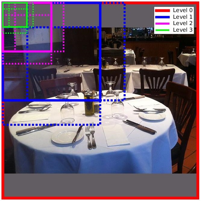
Using a hierarchical annocell structure has the advantage of allowing for coarse-to-fine exploration of the pose space. Note also that, by construction, annocells at low resolution are unions of certain high-resolution ones. This implies that the value of the annobits at low resolution can in turn be derived as maximums of high-resolution annobits.

4.3 Extended Existence Annobits

Due to the nature of the classifiers we use in our application, we also introduce annobits that list the categories that have entirely visible instances in an annocell, i.e., the collection

$$Y^{\mathit{cat}}_{A}=(Y_{C,A},C\in\mathcal{C}).$$ (13)

In addition, we also use category-independent, size-related annobits: For each annocell $A\!\in\!{\mathcal{A}}$ and size interval $M\!\in\!{\mathcal{M}}$, we define a binary annobit $Y^{\mathit{sc}}_{A,M}$ which indicates whether or not the average size of the objects present in $A$ belongs to $M$.

4.4 Classifiers for Annobits

The particular image-based predictors of the annobits we use in the table-setting application are described in full detail in section 8. Some examples include:

• Variables $X^{\mathit{cat}}_{A}$, $A\in\mathcal{A}$, which provide a vector of weights on $\mathcal{C}$ for predicting $Y^{\mathit{cat}}_{A}$.

• Variables $X^{\mathit{sc}}_{A}$, $A\in\mathcal{A}$, which provide a probability vector on $\mathcal{M}$ for predicting $(Y^{\mathit{sc}}_{A,M},M\in{\mathcal{M}})$.

Additional variables $X^{t}_{A},A\in\mathcal{A}^{\prime}$ (where $\mathcal{A}^{\prime}$ is a subset of $\mathcal{A}$) will also be introduced. They are designed to predict information units $Y_{A}^{t}=1$ if more than half of $A$ overlaps the table. Observe that the classifier $X_{q}$ assigned to $Y_{q}$ does not necessarily assume the same value as $Y_{q}$. However, this is not a problem since we are only interested in the conditional distribution of $X$ given $Y$.

5 Prior Model

Following section 3, the joint distribution of the annobits $(Y_{q},q\in\mathcal{Q})$ is derived from a prior model on the 3D scene description, $Z$, and on camera parameters $W$. We assume these variables to be independent and model them separately.

5.1 Scene Model $P(Z\,|\,S)$

Motivated by our application to dining room table scenes, we assume a fixed dominant plane in the 3D model, and choose a coordinate system $Oxyz$ in $\mathbb{R}^{3}$, such that the xy-plane coincides with this dominant plane. The scene $Z$ is represented as a set of object instances, assumed to be sitting on a bounded region of the dominant plane, in our case a centered, rectangular table $S$ characterized by its length and width. Recall from section 4.2 that each object instance $i$ is represented by a category $C_{i}\in\mathcal{C}$, a location $L_{i}$ and a size $D_{i}$ in the image. Here, we assume that objects from a given category have a fixed size, so that $Z=\{Z_{i}\}$ with $Z_{i}=(C_{i},L_{i})$. The distribution of $Z$ will be defined conditional to $S$, since, for example, the size of $S$ will directly impact the number of objects that it can support. More generally the table can be replaced by some other variable $S$ representing more complex properties of the global scene geometry. For convenience we sometimes drop $S$ from our notation. However, most of the model components introduced below depend on $S$, and the proposed model is to be understood conditional to $S$.

We partition the reference plane into small cells ($5\text{cm}\times 5\text{cm}$ in the table-setting case) and use binary variables to indicate the presence of instances of object categories centered in each cell. In other words, we discretize the family $(C_{i},L_{i})$ into a binary random field that we will still denote by $Z$. Letting $\mathcal{J}$ denote the set of cells, a configuration can therefore be represented as the binary vector $z=(z_{j,c},j\in\mathcal{J},c\in\mathcal{C})$ where $z_{j,c}=1$ if and only if an object of category $c$ is centered in the cell $j$.

The configuration $z$ is obviously a discrete representation of the scene layout restricted to object categories $\mathcal{C}$ and location $L$. Letting $\Omega$ denote the space of all such configurations, we will use a Gibbs distribution on $\Omega$ associated with a family of feature functions $\boldsymbol{\varphi}=(\varphi_{i},i=1,\ldots,n)$, with $\varphi_{i}:\Omega\mapsto\{0,1\}$, and scalar parameters $\boldsymbol{\lambda}=(\lambda_{i},i=1,\ldots,n)$. The Gibbs distribution then has the following form:

$$p(z)=\frac{1}{\kappa(\boldsymbol{\lambda})}\exp\bigl{(}\boldsymbol{\lambda}\cdot\boldsymbol{\varphi}(z)\bigr{)},$$ (14)

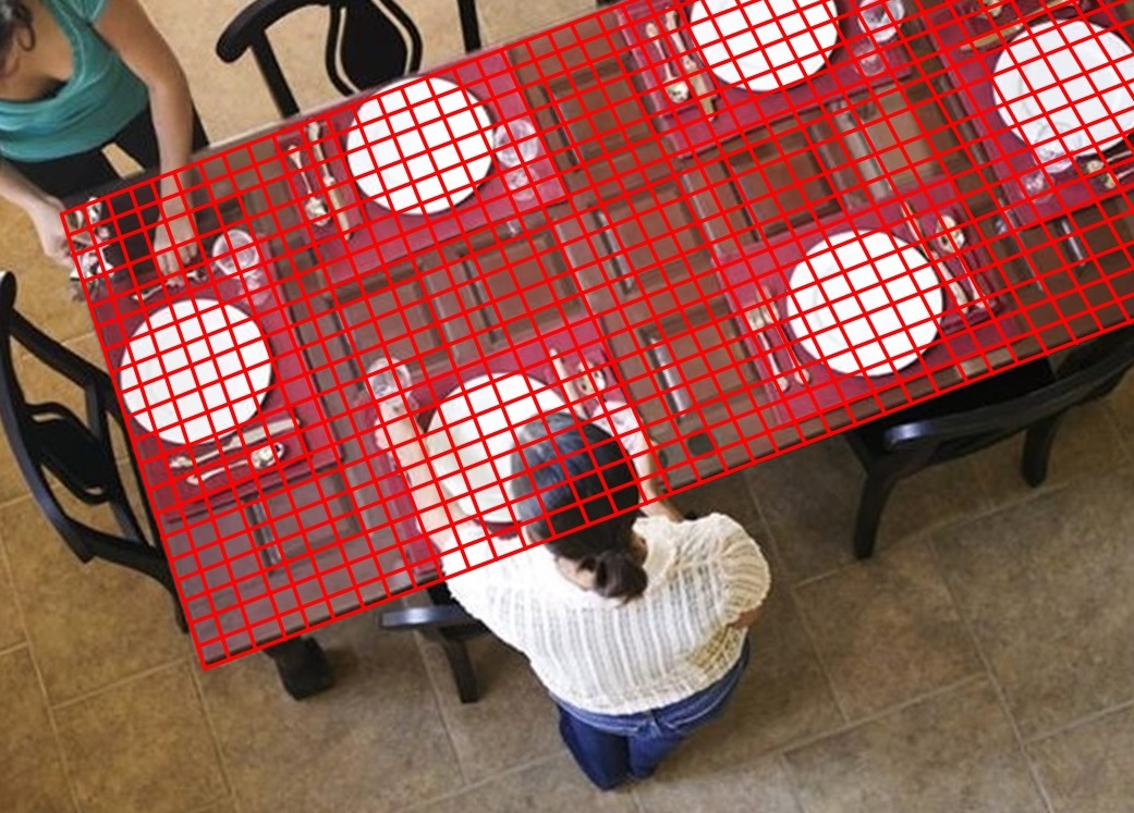
where $\kappa(\boldsymbol{\lambda})$ is the normalizing factor (partition function) ensuring that the probabilities sum up to one. Figure 2 shows a table and its fitted mesh where each of the cells is a $5\text{cm}\times 5\text{cm}$ square.

Figure 2: Table fitting mesh.

We use the following features:

• Existence features, which indicate whether or not an instance from a given category is centered anywhere in a given set of cells, therefore taking the form

  $$\varphi_{J,c}(z)=\max(z_{j,c},j\in J)$$ (15)

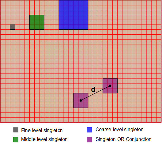
  with $J\subset\mathcal{J}$. We consider sets $J$ at three different granularity levels, illustrated in Figure 3. At the fine level $J=\{j\}$ is a singleton, so that $\varphi_{J,c}(z)=z_{j,c}$. We also consider middle-level sets (3$\times$3 array of fine cells) and coarse-level sets (6$\times$6 array of fine cells) that cover the reference plane without intersection.

• Conjunction features, which are products of two middle-level existence features (of the same or different categories), and therefore signal their co-occurrence:

  $$\varphi_{J_{1},c_{1},J_{2},c_{2}}(z)=\varphi_{J_{1},c_{1}}(z)\varphi_{J_{2},c_{2}}(z).$$ (16)

  To limit model complexity, only pairs $J_{1},J_{2}$ whose centers are less than a threshold away are considered where the threshold can depend on the pair $c_{1},c_{2}$.

Figure 3: Domain of various types of feature functions.

Invariance and symmetry assumptions about the 3D scene are then encoded as equality constraints among the model parameters thereby reducing model complexity. Grouping binary features $\varphi_{i}$ with identical parameters $\lambda_{i}$ is then equivalent to considering a new set of features that count the number of layout configurations satisfying some conditions on the locations and categories. For table settings, it is natural to assume invariance by rotation around the center of the table. Hence we assume that existence features whose domain $J$ is of the same size and located at the same distance from the closest table edge all have the same weights ($\lambda$’s), and hence the probability only depends on the number of such instances.

We group conjunction feature functions based on the distance of the first patch to the edge of the table, and the relative position of the second patch (left, right, front, or back) with respect to the first patch.

Remark 1

: The model can be generalized to include pose attributes other than location, e.g., orientation, size and height. If $\Theta$ denotes the space of poses, then one can extend the state space for $z_{j,c}$ to $\{0,1\}\times\Theta$, interpreting $z_{j,c}=(1,\theta)$ as the presence of an object with category $c$ and pose $\theta$ in cell $j$, and $z_{j,c}=(0,\theta)$ as the absence of any object with category $c$, $\theta$ being irrelevant. Features can then be extended to this state space to provide a joint distribution that includes pose. The simplest approach would be to only extend univariate features, so that object poses and other attributes are conditionally independent given their categories and locations (and the geometry variable $S$, since the model is always assumed conditional to it). Other attributes (color, style, etc.) can be incorporated in a similar way.

5.2 Camera Model $P(W)$

The second component of the prior model determines the probability distribution of the extrinsic and intrinsic camera parameters, such as its pose and focal length, respectively. The definition of these parameters is fairly standard in computer vision (see e.g., Ma et al. (2003)), but the definition of generative models for these parameters is not. In what follows we summarize the typical definitions, and leave the details of the generative model to the Appendix.

Remember that we assumed a fixed coordinate system in 3D in which the $xy$-plane coincides with the dominant “horizontal” plane. Consider also a second camera coordinate system $O^{\prime}x^{\prime}y^{\prime}z^{\prime}$, such that $x^{\prime}y^{\prime}$-plane is equal to the image plane. The extrinsic camera parameters are defined by the pose $(R,T)$ of the camera coordinate system $O^{\prime}x^{\prime}y^{\prime}z^{\prime}$ relative to the fixed coordinate system $Oxyz$, where $R$ is the camera rotation, which maps the unit axis vectors of $Oxyz$ to the unit axis vectors of $O^{\prime}x^{\prime}y^{\prime}z^{\prime}$, and $T=OO^{\prime}$ is the translation vector. We parametrize the rotation $R$ by three angles $\boldsymbol{\psi}=(\psi_{x},\psi_{y},\psi_{z})$ representing, respectively, counter-clockwise rotations of the camera’s coordinate system about the x-axis, y-axis, and z-axis of the world coordinate system (see equation (29) for conversion of unit vectors to angles). Observe that one can express the coordinates $m=(x,y,z)^{\top}$ of a 3D point in the world coordinate system as functions of its coordinates in the camera coordinate system $m^{\prime}=(x^{\prime},y^{\prime},z^{\prime})^{\top}$ in the form $m=Rm^{\prime}+T$. Since in our case 3D points lie in a plane $N^{\top}m^{\prime}=d$, where $N$ is the normal to the plane (i.e., table) measured in the camera coordinate system and $d$ is the distance from the plane to the camera center, we further have $m=Hm^{\prime}$, where $H=(R+TN^{\top}/d)$ is the homography between the camera plane and the world plane.

The intrinsic camera parameters are defined by the coordinates of the focal point, $(x_{0},y_{0},-f)$, where $f>0$ is the focal length and $(x_{0},y_{0})$ is the intersection of the principal axis of the camera with the image plane, as well as the pixel sizes in directions $x^{\prime}$ and $y^{\prime}$, denoted by $\gamma_{x}$ and $\gamma_{y}$.

The complete set of camera parameters is therefore 11-dimensional and given by $W=(f,\gamma_{x},\gamma_{y},x_{0},y_{0},\boldsymbol{\psi},T)$. Our generative model for $W$ assumes that:

• Intrinsic camera parameters are independent from extrinsic camera parameters.

• Pixels are square, i.e., $\gamma_{x}=\gamma_{y}$, but intrinsic parameters are otherwise independent. The focal length $f$ is uniformly distributed between 10 and 40 millimeters, $x_{0}$ (resp. $y_{0}$) is uniformly distributed between $W_{p}/4$ and $3W_{p}/4$ (resp. $H_{p}/4$ and $3H_{p}/4$), where $W_{p}$ and $H_{p}$ are the width and height of the image in pixels, and $\gamma_{x}=\gamma_{y}$ is uniformly distributed between $1/W_{p}$ and $1.2/W_{p}$.

• The vertical component of $T$ is independent of the other two and the distribution of the horizontal components is rotation invariant. Specifically, letting $T=(T_{x},T_{y},T_{z})$, we assume that $(T_{z}-0.3)/2.7$ follows a Beta distribution so that $T_{z}\in[0.3,3]$ (expressed in meters). Then, letting $r=\sqrt{T_{x}^{2}+T_{y}^{2}}$ denote the distance between the horizontal projection of $T$ on the table plane and the center of the table, we assume that $r/4$ follows a Beta distribution. We assume independence of $r$ and $t_{z}$ and invariance by rotation around the vertical axis, which specifies the distribution of $T$.

• The distribution of the rotation angles $\mathbf{\psi}$ is defined conditionally to $T$. Specifically, we assume that the camera roughly points towards the center of the scene and the horizontal direction in the image plane is also horizontal in the 3D coordinate system. Additional details of the model for $p(\psi|T)$ are provided in the Appendix.

5.3 Scene Geometry Model $P(S)$ and Global Model

We assume that the scene geometry $S$ takes value in a finite set of “template geometries” that coarsely cover all possible situations. Note that these templates are defined up to translation, since we can always assume that the 3D reference frame is placed in a given position relative to the geometry. For table settings, where the geometry represents the table itself, our templates were simply square tables with size distributed according to a shifted and scaled Beta distribution ranging from 0.5 to 3 meters. This rough approximation was sufficient for our purposes, even though tables in real scenes are obviously much more variable in shape and size.

Finally, the joint prior distribution $p(z,s,w)=P(Z=z,S=s,W=w)$ of all the variables is defined by:

$$p(z,s,w)=p(z|s)~{}p(s)~{}p(w).$$ (17)

5.4 Learning the Prior Model

The models for $P(S)$ and $P(W)$ are simple enough that we specified their model parameters manually, as described before. Therefore, the fundamental challenge is to learn the prior model on scene interpretations $P(Z\,|\,S)$. For this purpose, we assume that a training set of annotated images is available. The annotation for each image consists of a list of object instances, each one labeled by its category (and possibly other attributes) and apparent 2D pose represented by an ellipse in the image plane. We also assume that sufficient information is provided to propagate the image annotation to a scene annotation in 3D coordinates; this will allow us to train the scene model independently from the unknown transformation that maps it to the image. This can be done in several ways. For example, given four points in the image that are the projections of the corners of a square in the reference plane, one can reconstruct, up to a scale factor, the homography mapping this plane to the image. Doing this with a reasonable accuracy is relatively easy in general for a human annotator, and allows one to invert the outline of every flat object on the image that lies on the reference plane to its 3D shape, up to a scale ambiguity. This ambiguity can be removed by knowing the true distance between two points in the reference plane, and their positions in the image. We used this level of annotation and representation for our table settings, based on the fact that all objects of interest were either horizontal (e.g., plates), or had easily identifiable horizontal components (e.g., bottoms of bottles), and we assumed that plates had a standard diameter of 25cm to remove the scale ambiguity.

As can be seen, the level of annotation required to train our prior model is quite high. While we have been able to produce rich annotations for 3,000 images of dining room table settings (see section 9), this is insufficient to train our model. To address this issue, in the next section we propose a 3D scene generation model that can be use to generate a large number of annotations for as many synthetic images as needed. Given the annotations of both synthetic images (section 6) as well as real images (section 9), the parameters of our prior model are learned using an accelerated version of the robust stochastic approximation (Nemirovski et al., 2009) to match empirical statistics calculated based on top-down samples from the scene generation model (see Jahangiri (2016) for details).

6 Scene Generation Model

In this section we propose a 3D scene generation model that can be used to generate a large number of annotations to train the prior model described in the section 5. The proposed model mimics a natural sequence of steps in composing a scene. First, create spontaneous instances by placing some objects randomly in the scene; the distribution of locations depends on the scene geometry. Then, allow each of these instances to trigger the placement of ancillary objects, whose categories and attributes are sampled conditionally, creating groups of contextually related objects. This recursive process terminates when no children are created, or when the number of iterations reaches an upper-bound.

6.1 Model Description Using a Generative Attributed Graph

To formally define this process, we will use the notation $\mathbf{n}=(n_{c},c\in\mathcal{C})$ to represent a family of integer counts $n_{c}\in\mathbb{N}$ indexed by categories, so that $\mathbf{n}\in\mathbb{N}^{|\mathcal{C}|}$. We will also let $|\mathbf{n}|=\sum_{c\in\mathcal{C}}n_{c}$.

We will assume a probability distribution $p^{(0)}$ on $\mathbb{N}^{|\mathcal{C}|}$, and a family of such distributions $p^{(c)},c\in\mathcal{C}$. These distributions (which are defined conditionally to $S=s$) are used to decide the number of objects that will be placed in the scene at each step. More specifically:

1. $p^{(0)}(\cdot\,|\,s)$ is the conditional joint distribution of the number of object instances from each category that are placed initially on the scene.

2. For each category $c\in\mathcal{C}$, $p^{(c)}(\cdot\,|\,s)$ is the joint distribution of the numbers of new object instances that are triggered by the addition of an object instance from category $c$. These distributions can be thought of as the basis distributions in a multi-type branching process (see Mode (1971)).

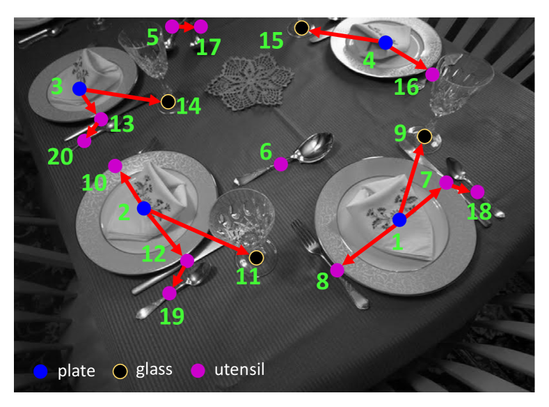
The complexity of the process is controlled by a master graph that restricts the subset of categories that can be created at each step. More formally, this directed graph has vertices in $\{0\}\cup\mathcal{C}$ and is such that $p^{(v)}$ is supported by categories that are children of the node $v\in\{0\}\cup\mathcal{C}$. Adjoining $0$ to the node labels avoids treating $p^{(0)}$ as a special case in the derivations below. The master graph we used on table settings is provided in Figure 4, where we regard “plate” and “bottle” as the children of category $0$. Note that since we allow spontaneous instances from all categories every category is a child to category 0.

Figure 4: An example master graph.

The output of this branching process can be represented as a directed tree $G_{0}=(V,C,E)$ in which each vertex $v\in V$ is attributed a category denoted by $C(v)$ and $E$ is a set of edges. The root node of the tree, hereafter denoted by $0$, essentially represents the empty scene whose “category” is also denoted by 0 (note that $0\not\in\mathcal{C}$). All other nodes have categories in $\mathcal{C}$. Each non-terminal node $v\in V$ has $|\mathbf{N}^{(v)}|$ children where $\mathbf{N}^{(v)}\sim p^{(c(v))}(\cdot|s)$ so that $N_{c}^{(v)}$ of these children have category $c$. We will refer to $G_{0}$ as a skeleton tree, which needs to be completed with the object attributes (excluding its category since $G_{0}$ already includes the category attribute) to obtain a complete scene description. The probability distribution of $G_{0}$ is

$$p(G_{0}\,|\,s)=\prod_{v\in V\backslash V_{T}}p^{(c(v))}(\mathbf{n}^{(v)}\,|\,s),$$ (18)

where $V_{T}$ is the set of terminal nodes and $\mathbf{n}^{(v)}$ are the category counts of the children of $v$ (graphs being identified up to category-invariant isomorphisms). An example of such graph is provided in Figure 5.

Figure 5: A table-setting scene (top) and its corresponding skeleton graph (bottom) where the categories (plate, bottle, glass, and utensil) are color-coded in the graph. Root nodes $V_{0}$ initialize the generative process; here there are six. The terminal nodes for this instance are $V_{T}=\{6,8,9,10,11,14,15,16,17,18,19,20\}$. According to the base graph $n^{(0)}_{\text{plate}}=4$,$n^{(0)}_{\text{bottle}}=0$, $n^{(0)}_{\text{glass}}=0$ and $n^{(0)}_{\text{utensil}}=2$.

To complete the description, we need to associate attributes to objects, the most important of them being their poses in the 3D world, on which we focus now. In the MRF designed for our experiments, the only relevant information about pose was the location on the table, a 2D parameter. It is however possible to design a top-down generative model that includes richer information, using for example a 3D ellipsoid. Such representations involve a small number of parameters denoted generically by $\theta$: each vertex $v$ in the skeleton graph is attributed by parameters such as its pose denoted by $\theta^{(v)}$. When using ellipsoids, $\theta^{(v)}$ involves eight free parameters (five for the shape of the ellipsoid, which is a positive definite symmetric matrix, and three for its center). Fewer parameters would be needed for flat objects (represented by a 2D ellipse), or vertical ones, or objects with rotational symmetry. In any case, it is obvious that the distribution of an object pose depends heavily on its category.

In our model, contextual information is important: when placing an object relative to a parent, the pose also depends on the parent’s pose and category. This is captured by the conditional distribution $p^{(c)}(\theta\,|\,c^{\prime},\theta^{\prime})$ of the pose parameters for a category $c$, relative to a parent with category $c^{\prime}$ and pose $\theta^{\prime}$. To simplify notation, we allow again for $c^{\prime}=0$ (indicating objects without parent), in which case $\theta^{\prime}$ is irrelevant. The complete attributed graph associated with the scene is now $G=(V,C,\Theta,E)$ (where $\Theta$ is the family of poses) with distribution

$$p(G=g|s)=\prod_{v\in V\backslash V_{T}}p^{(c(v))}(\mathbf{n}^{(v)}|s)\\ \prod_{v\in V\setminus\{0\}}p^{(c(v))}(\theta^{(v)}|c(pa(v)),\theta_{pa(v)}),$$ (19)

where $pa(v)$ is the parent of $v$. In (19), we have mixed discrete probability mass functions for the object counts and continuous probability density functions for the pose attributes.

If one is only interested in the objects visible in the scene, the scene description, $Z$, is obtained by discarding the graph structure from $G$, i.e., only retaining the object categories and poses. More complex scene descriptors could be interesting as well, like object relationships or groupings (e.g., whether a family of plate, utensils, glasses can be considered as belonging to a single setting), in which case the whole graph structure may also be of interest; we do not use such “compositions” in our experiments. As a final point, we mention that the samples may require some pruning at the final stage, since the previous model does not avoid object collisions or overlaps that one generally wants to avoid. We removed physically impossible samples in which vertical object categories (i.e., bottle and glass) were overlapping in the world coordinate system. In general, one can add undirected edges between the children of the same parent to incorporate more context into a single setting. More details on the scene model that we used for table-settings can be found in the Appendix.

6.2 Algorithm for Learning the Scene Generation Model

Even though the annotation is assumed to describe the scene in the world coordinate system, the information it provides on $G$ is still incomplete, because it does not include the graph structure. To learn the parameters of the branching process, we used the EM algorithm (Dempster et al., 1977) or, more precisely, the Monte-Carlo version of the Stochastic Expectation-Maximization (SEM) algorithm (Celeux and Diebolt, 1985), usually referred to as MCEM in the literature (Wei and Tanner, 1990). In this framework, the conditional expectation of the complete log-likelihood, which is maximized at each step to update the parameters, is approximated by Monte-Carlo sampling, averaging a sufficient number of realizations of the conditional distribution of the complete data given the observed one for the current parameters. Note that the unobserved part of the graph given $(V,C,\Theta)$ can be represented as a $|V|$-dimensional vector $\boldsymbol{\zeta}=\bigl{(}\zeta_{1}=pa(v_{1}),\zeta_{2}=pa(v_{2}),...,\zeta_{|V|}=pa(v_{|V|})\bigr{)}$, with $pa(v)=\emptyset$ if $v$ is an orphan. These configurations form a subset of $V\cup\{\emptyset\}$, given the constraints imposed by the master graph and the fact that $g$ is acyclic. The Gibbs sampling algorithm iteratively updates each $\zeta_{i}$ according to its conditional distribution given the observed variables and the other $\zeta_{j}$, $j\neq i$, which can easily be computed using equation (19). Recall that the graph distribution is learned conditional to a given scene geometry $S=s$.

6.3 Simulated Table Settings

Figure 6: Top-view icon visualization of table-settings considering only plate, bottle, glass, utensil categories. Upper Panel: visualization of some annotated images in the dataset that roughly match in size to a $1.5\times 1.5\hskip 1.42262ptm^{2}$ table Lower Panel: samples from the generative attributed graph model for a square table of size $1.5\times 1.5\hskip 1.42262ptm^{2}$.

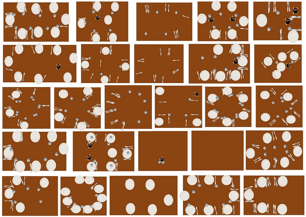
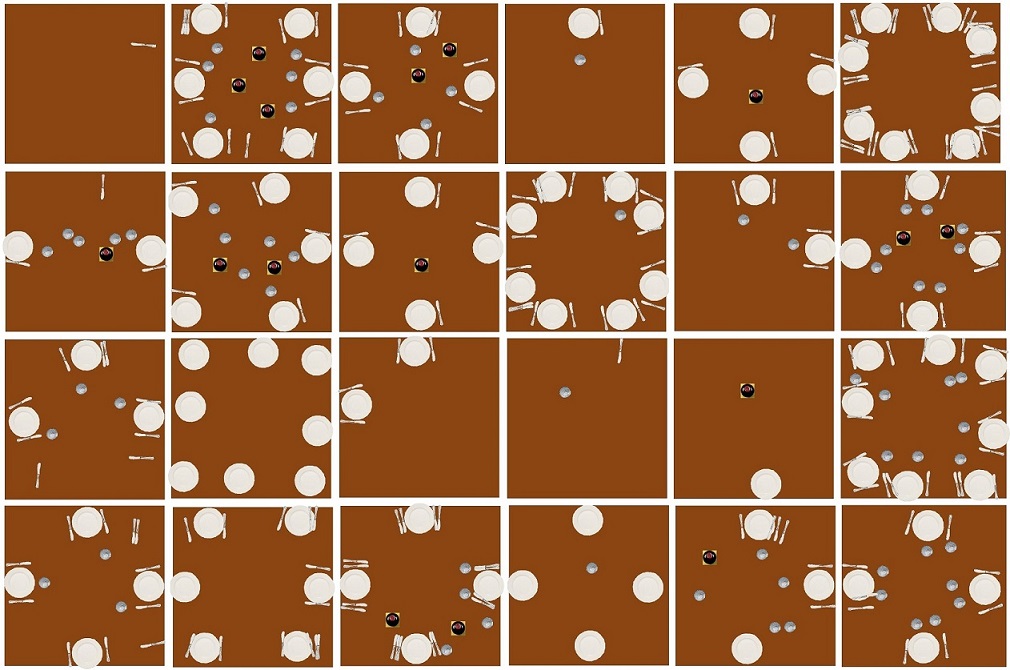
Figure 6 shows top-view visualization of some annotated images in the dataset that roughly match in size to a $1.5\times 1.5\hskip 1.42262ptm^{2}$ table and some samples drawn from the generative attributed graph model for a square table of size $1.5\times 1.5\hskip 1.42262ptm^{2}$ learned from matching annotated images. Visual similarity of the samples taken from the generative attributed graph model to natural scene samples confirm suitability of this model for table setting scenes although the proposed model is quite general and can be used to model different types of scenes.

Remark 2

: We developed algorithms for unconditional and conditional sampling of the graph model in the context of IP (the conditional distribution relative to the current history). The unconditional sampling is top-down, easy and fast. However, our conditional sampling based on Metropolis-Hastings (Hastings (1970); Metropolis et al. (1953)) is relatively complex and slow to adapt to a new condition i.e., long burn-in period; this is partly due to the innate low acceptance rate of the Metropolis-Hastings algorithm, normally $<25\%$ (see Roberts and Rosenthal (2001) and Jahangiri (2016) for details). This is why we have not used this model directly in the IP framework, relying instead on the MRF model described in section 5.1, in which the feature expectations are learned on scenes generated by the generative attributed graph model.

7 Conditional Sampling

Sampling from the posterior distribution over hidden variables given evidence is central to our method, being necessary for both IP and performance evaluation. Writing $\Xi=(Z,S,W)$ for the unobserved scene-related variables, the prior distribution $p(\xi)=p(z,s,w)$ was given in (17). Recall that the annobits $Y_{q}$ are deterministically related to the scene, with $Y_{q}=f_{q}(Z,W)$. In this discussion, we will work under the simplifying assumption that the classifiers are conditionally independent given $\Xi$ and that, for a given $q$, the conditional distribution of $X_{q}$ given these variables only depends on $Y_{q}$. (This assumption can be relaxed to a large extent without significantly increasing the complexity of the algorithm. This will be discussed at the end of this section.) Recall also (see Section 3.2) that at step $k$ of IP, in order to compute the conditional mutual information and determine the next query $q_{k}$, we require the mixture weights $P(Y_{q}=y|\mathbf{E}_{k-1})$, where $\mathbf{E}_{k-1}=\{X_{q_{1}}=x_{1},...,X_{q_{k-1}}=x_{k-1}\}$ is the evidence after $k-1$ steps. Clearly, then, $P(Y_{q}=y|\mathbf{E}_{k-1})$ can be estimated from samples from $\Xi$ given the history.

The joint distribution of $\Xi$ and all the data $X_{\mathcal{Q}}$ therefore takes the form

$$P(x_{\mathcal{Q}},\xi)=p(z\,|\,s)p(w)p(s)\prod_{q\in\mathcal{Q}}p(x_{q}\,|\,f_{q}(z,w)).$$ (20)

Since the next query $q_{k}$ is a deterministic function of $\mathbf{E}_{k-1}$, the conditional distribution of $\Xi$ given $\mathbf{E}_{k-1}$ is

$$p(\xi\,|\,\mathbf{E}_{k-1})\propto p(z\,|\,s)p(w)p(s)\prod_{q=1}^{k-1}p(x_{q}\,|\,f_{q}(z,w)),$$ (21)

for which we have again used the conditional independence of the $X_{q}$’s given the scene.

7.1 General Framework

We use a Metropolis-Hastings sampling strategy to estimate the conditional distribution of the scene variables given the history. As a reminder, the algorithm relies on the fact that any transition probability $\psi(\xi,\xi^{\prime})$ can be modified by rejection sampling to be placed in detailed balance with $p(\xi\,|\,\mathbf{E}_{k-1})$ by letting

$$\psi^{*}(\xi,\xi^{\prime})=\\ \begin{cases}\displaystyle\psi(\xi,\xi^{\prime})\max\left(1,\frac{\psi(\xi^{\prime},\xi)p(\xi^{\prime}\,|\,\mathbf{E}_{k-1})}{\psi(\xi,\xi^{\prime})p(\xi\,|\,\mathbf{E}_{k-1})}\right),\\ \displaystyle\hskip 108.405pt\text{ if }\xi^{\prime}\neq\xi\\ \displaystyle 1-\sum_{\xi^{\prime\prime}\neq\xi}\psi^{*}(\xi,\xi^{\prime\prime}),\text{ if }\xi^{\prime}=\xi\end{cases}$$ (22)

provided $\psi(\xi,\xi^{\prime})>0\Rightarrow\psi(\xi^{\prime},\xi)>0$. The Metropolis-Hastings strategy assumes a family of “elementary moves” represented by transition probabilities $\{\psi_{m}(\xi,\xi^{\prime})\}$. At each step, say $t$, of the algorithm, a move $m_{t}$ is chosen (based on a random or deterministic scheme), and a new configuration is created with probability $\psi_{m_{t}}^{*}(\xi_{t-1},\cdot)$, where $\xi_{t-1}$ is the current configuration. The set of elementary moves and the updating scheme must be chosen appropriately to ensure that the chain is ergodic.

7.2 Application to the Scene Model

The feasibility of the method relies on whether the ratio intervening in (22) is tractable. In this equation, all terms can be relatively easily computed, with the exception of the probabilities $p(z|s)$ in (21) because of the normalizing constant in (14) which depends on $s$. This constant cancels in the ratio whenever the values of $s$ in $\xi$ and $\xi^{\prime}$ coincide, i.e., the elementary move does not change the scene geometry. Among moves that satisfy this property, moves involving the camera properties $w$ are generally computationally demanding, because they modify all the annobits, while elementary changes in $z$ only have a local impact.

7.2.1 Changing the Scene Geometry

To process moves that modify $s$, the normalizing constant in (14), namely

$$\kappa(\boldsymbol{\lambda})=\sum_{z\in\Omega}\exp(\boldsymbol{\lambda}\cdot\boldsymbol{\varphi}(z))$$ (23)

must be computed (where $\boldsymbol{\lambda},\Omega$ and $\boldsymbol{\varphi}$ all depend on $s$). Whereas an exact computation is intractable, approximations can be obtained, using, for example, the formula

$$\log\kappa(\boldsymbol{\lambda})=\log\kappa(\boldsymbol{\lambda}_{0})\\ +\int_{0}^{1}\!\!\!E\Big{(}(\boldsymbol{\lambda}-\boldsymbol{\lambda}_{0})\cdot\boldsymbol{\varphi}\,|\,\boldsymbol{\lambda}_{0}+t(\boldsymbol{\lambda}-\boldsymbol{\lambda}_{0})\Big{)}dt$$ (24)

in which $\boldsymbol{\lambda}_{0}$ is a parameter at which $\kappa$ is computable (typically making all variables independent) and each expectation in a numerical approximation of the integral is computed using Monte-Carlo sampling. This is a costly but can be computed offline for each value of $s$ (which can be discretized over a finite set).

In our application, however, we have used a simpler approach, relying on a good estimator of $S$ that is fixed in the rest of the computation. Letting $\hat{S}$ be this estimator, we sampled $S$ over a small neighborhood of $\hat{S}$, making the additional approximation that $\kappa$ in constant (as a function of $s$) in this neighborhood.

7.2.2 Changing the Camera Properties

For the camera properties, we use a proposal distribution taking the form $\psi_{W}(\xi,\xi^{\prime})=p(w^{\prime}|I)$, where the $z$ and $s$ coordinates in $\xi$ and $\xi^{\prime}$ coincide, and $I$ is the observed image. The dependency on $I$ is implemented through an estimator limiting the camera parameters, which will be described in the next section. The proposal distribution of $S$ can be assumed to be uniform over the finite set of scene geometries which is considered.

7.2.3 Changing object indicators

In our implementation, in which $z=\{z_{j}\}$ is a collection of binary variables, elementary moves correspond to Gibbs sampling, taking,

$$\psi_{j}(\xi,\xi^{\prime})=p(z^{\prime}_{j}\,|\,\mathbf{E}_{k-1},\{z_{l}\hskip 1.42262pt,l\neq j\})$$

if $\xi=(z,w,s)$ and $\xi^{\prime}=(z^{\prime},w^{\prime},s^{\prime})$ are such that $w=w^{\prime}$, $s=s^{\prime}$ and $z_{l}=z^{\prime}_{l}$ for $l\neq j$; and taking $\psi_{j}(\xi,\xi^{\prime})=0$ in all other cases.

The overall updating scheme is based on nested loops, where the inner loop updates $z$, the middle one updates $w$ and the outer one $s$. Each loop is run several times before an update is made at a higher level.

8 Classifiers and Data Model

We trained three deep CNNs. The first one, “CatNet,” is for object category classification; the second one, “ScaleNet,” is to estimate the size of detected object instances, and the third, “SceneNet,” is to estimate the scene geometry in a given image. All of these CNNs borrow their network architecture, up to the last weight layer, i.e., layer 15, from the VGG-16 network (Simonyan and Zisserman, 2014). The last fully-connected layer (16-th weight layer) and the following softmax layer of these three CNNs were modified to accommodate our design needs. All CNNs rely on “transfer learning” by initializing the first 15 weight-layers to the corresponding weights from the VGG-16 network trained on 1.2 million images from the ImageNet dataset (see Deng et al. (2014)). However, since the last layer’s architecture for all three CNNs is different from VGG-16, the corresponding weights were randomly initialized during training. All CNNs were trained and tested using the Caffe Deep Learning framework (Jia et al., 2014) using an Nvidia Tesla K40 GPU on a desktop computer with Intel i7-4790K Quad-Core processor (8M Cache and up to 4.40 GHz clock rate) and 32-GB RAM running Ubuntu 15.04 operating system. The processing time for each patch is about 12 seconds on our end-of-the-line Intel i7-4790K CPU and 0.2 seconds on the Tesla K40 GPU. Since the input patches are of the same size, namely $224\times 224$, and pass through the same network, the classifiers all have the same computational cost during test time. We describe the design, training, and performance of these CNNs in the following subsections.

8.1 CatNet

For each object category $c\in\mathcal{C}$, we want to detect if there is at least one instance in a given patch $A$. This will be done simultaneously for all categories, including “background.” Moreover, all patches are resized to $224\times 224$ and only one CNN is trained independently of the original size of $A$ in the image. This suffices in our framework since patches are restricted to the 4-level annocell hierarchy and the smallest annocells remain at the scale of objects except in extreme cases. CatNet is then a CNN with a softmax output layer, which returns a vector of scores $X^{\mathit{cat}}=(X^{\mathit{cat}}_{c},c\in\mathcal{C}\cup\{0\})$, where each $X^{\mathit{cat}}_{c}$, for $c\in\mathcal{C}$, reflects a proportional confidence level about the presence of at least one object from category $c$ in the patch, while $X^{\mathit{cat}}_{0}$ corresponds to an empty patch (or the ”No Object” category). The scores are non-negative and sum to 1, but they should not be interpreted as probability of existence, since the events they represent are not incompatible i.e., they can co-occur.

The corresponding annobit $Y^{\mathit{cat}}_{A}$ is a binary vector $Y^{\mathit{cat}}_{A}=(Y^{\mathit{cat}}_{c,A},c\in\mathcal{C})$ where $Y^{\mathit{cat}}_{c,A}=1$ if and only if an object with category $c$ exists in $A$. The conditional distribution $P(x^{\mathit{cat}}|y^{\mathit{cat}})$ is taken to be independent of $A$, and modeled as a Dirichlet distribution separately for each of the $2^{|\mathcal{C}|}$ possible configurations of $Y^{\mathit{cat}}$. We used a fixed-point (without projection) iterative schemes to perform MLE parameter estimation (see Minka (2012)).

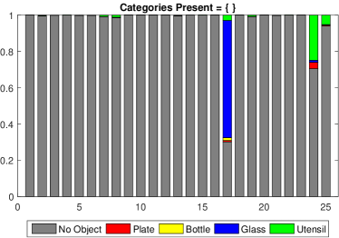
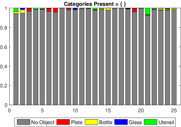
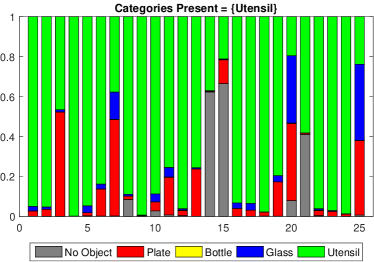
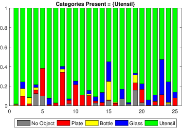
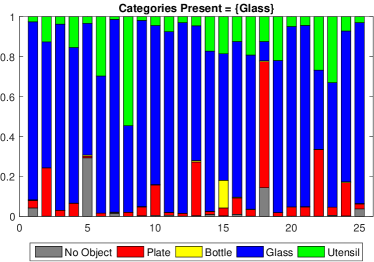
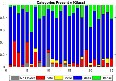
Figure 7 illustrates some samples from the learned Dirichlet distribution versus some sample CNN outputs for the corresponding annobit $Y^{cat}$ for a few configurations. We have $|\mathcal{C}|=4$ and therefore estimated 16 conditional distributions. The figure shows stacked bar visualization of 25 samples (per configuration) drawn randomly from data collected by running CatNet on patches (left column) and samples taken from the Dirichlet model learned from CatNet output data (right column) where each row corresponds to one of the 16 annobit configurations. We have shown stacked bars for only four configurations as example. The length of each colored bar represent the proportion of each category; therefore, the total length of each stacked bar is equal to 1. Two interesting observations are: (1) the length of bars corresponding to the present categories are comparable and usually considerably larger than the length of absent categories; (2) the color distribution of CatNet outputs and Dirichlet model samples are very similar for the same configuration. This supports the argument for using a Dirichlet distribution in modeling the data distribution $p(x^{\mathit{cat}}|y^{\mathit{cat}})$. Stacked bars are good means to visually inspect and compare the true empirical distribution versus the Dirichlet model.

  
  
  
  

Figure 7: Stacked bar visualization of samples from CatNet output (left) and Dirichlet model (right).

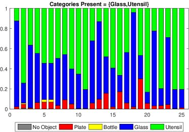
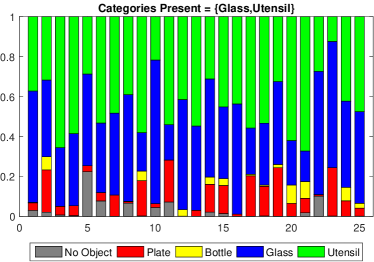
8.2 ScaleNet

Figure 8: Scale ratio intervals.

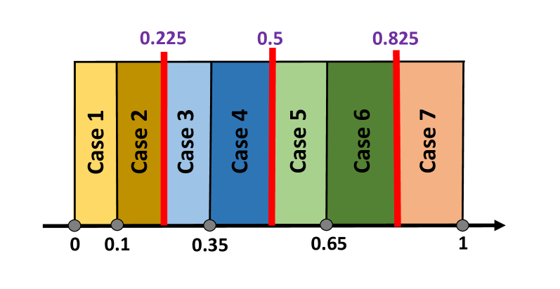
Define the scale of an object in an image patch as the ratio of its longest side to the patch size (therefore belonging to $(0,1]$ when completely visible. The ScaleNet predictor is designed to estimate the average scale of object instances in a given patch, independent of their category.

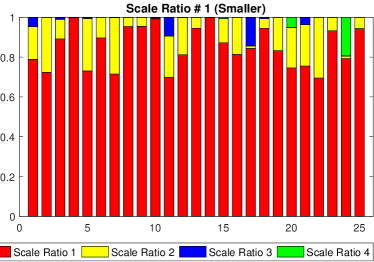
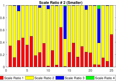
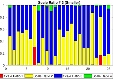
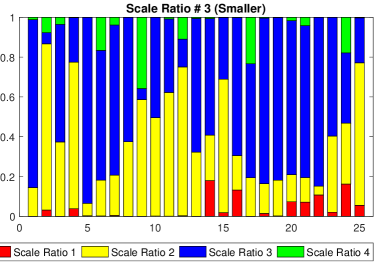
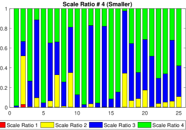
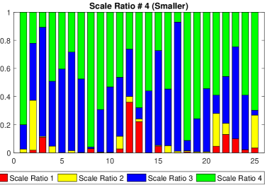
Assume a quantization $(\tau_{0}=0,\tau_{1},\ldots,\tau_{d-1},\tau_{d}=1)$ of the unit interval (in our experiments, we used $d=4$ and quantization levels of $0.1$, $0.35$, $0.65$, and $1$). We modified the VGG-16 network by assigning $d$ output values to the softmax layer and trained by assigning to each patch in the training data the index $j\geq 1$ such that $\tau_{j}$ is closest to the average scale of the objects it contains, using only non-empty patches. The output of the CNN is a vector $X^{\mathit{sc}}=(X^{\mathit{sc}}_{1},\ldots,X^{\mathit{sc}}_{d})$ of non-negative weights summing to one. Again, there is only one CNN and patches of different sizes are aggregated for training. The associated annobit $Y^{\mathit{sc}}\in\{1,2d-1\}$ is the index of the Voronoï cell that contains the average scale, obtained by adding midpoints $\tau_{j+1/2}=(\tau_{j}+\tau_{j+1})/2$ to the initial sequence (which separates the unit interval into $2d-1$ regions; see Figure 8). The conditional distribution $P(x^{\mathit{sc}}|y^{\mathit{sc}})$ is then modeled and trained as a Dirichlet distribution for each value $y^{\mathit{sc}}=1,\ldots,2d-1$.

Figure 9 (similar to Figure 7) provides some ScaleNet stacked bars visualizations for 4 (out of $2d-1=7$) scale configurations.

  
  
  
  

Figure 9: Stacked bar visualization of samples from ScaleNet output (left) and Dirichlet model (right).

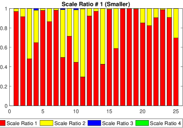
8.3 SceneNet

SceneNet combines binary classifiers predicting whether or not an input patch belongs to the dominant plane. The basic architecture is the same as that of the CatNet and ScaleNet. It returns a region $\hat{M}$ in the image plane. For a given scene geometry $s$ and camera properties $w$, let $M(s,w)$ be the representation of $s$ in the image plane. We discretize the image plane into non-overlapping patches, and let $\mathbf{X}^{g}=(X^{g}_{j},j=1,\ldots,m_{t})$ be the corresponding SceneNet outputs. Let $Y^{g}_{j}=1$ if the corresponding patch belongs to $M(s,w)$ and zero otherwise.

9 JHU Table-Setting Dataset

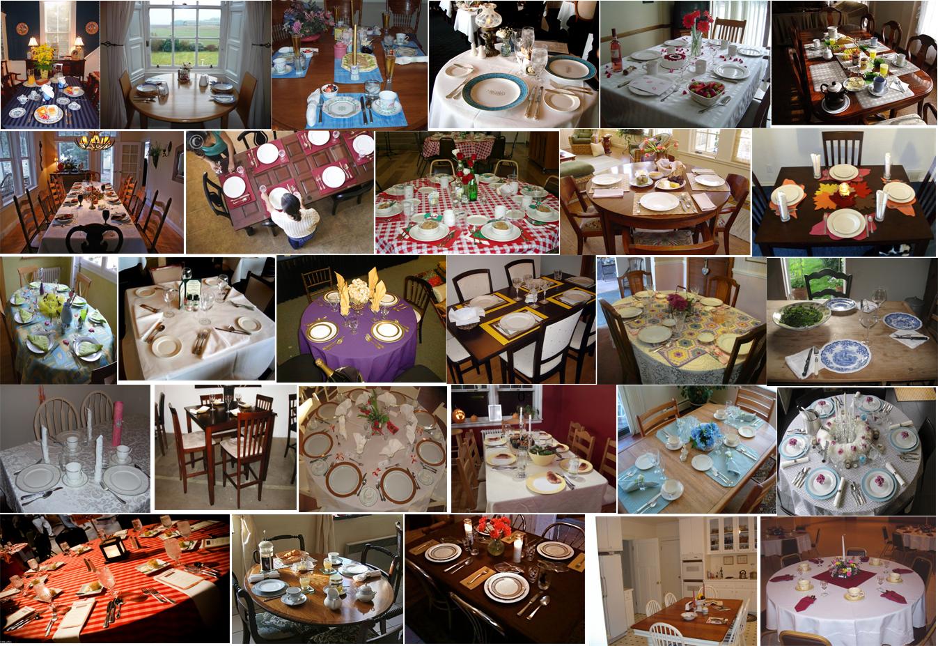
We collected and annotated the “JHU Table-Setting Dataset,” which consists of about 3000 images of dining room table settings with more than 30 object categories. The images in this dataset were collected from multiple sources such as Google, Flickr, Altavista, etc. Figure 13 shows a snapshot of the dataset, which is made publicly available .

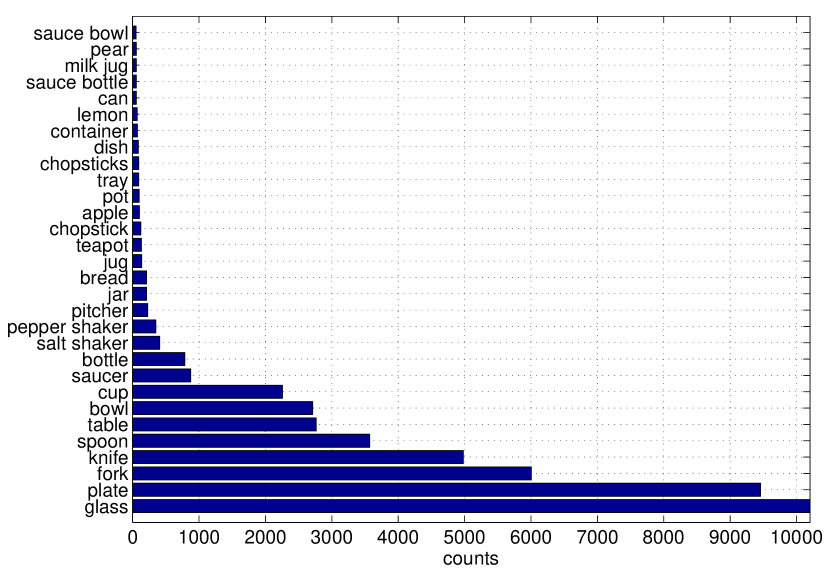
The images were annotated by three annotators over a period of about ten months using the “LabelMe” online annotating website  Russell et al. (2008). The consistency of labels across annotators was then verified and synonymous labels were consolidated. The annotation task was carried out with careful supervision resulting in high quality annotations, better than what we normally get from crowd-sourcing tools like Amazon Mechanical Turk. Figure 13 shows the annotation histogram of the 30 most annotated categories. The average number of annotations per image is about 17.

Figure 10: A snapshot of the JHU Table-Setting Dataset.

Figure 11: The number of annotated instances of each object category in the whole dataset for the 30 top most annotated object categories.

Figure 12: Rectification of table surfaces after back-projection.

Figure 13: Left: an annotated image from the table-setting dataset. Middle: back-projection of table (in blue), plates (in red), glasses (in green), and utensils (in black). The unit of axes is centimeter. Right: top-view visualization of the table-setting (all utensil instances including fork, knife, and spoon are shown by knife icon).

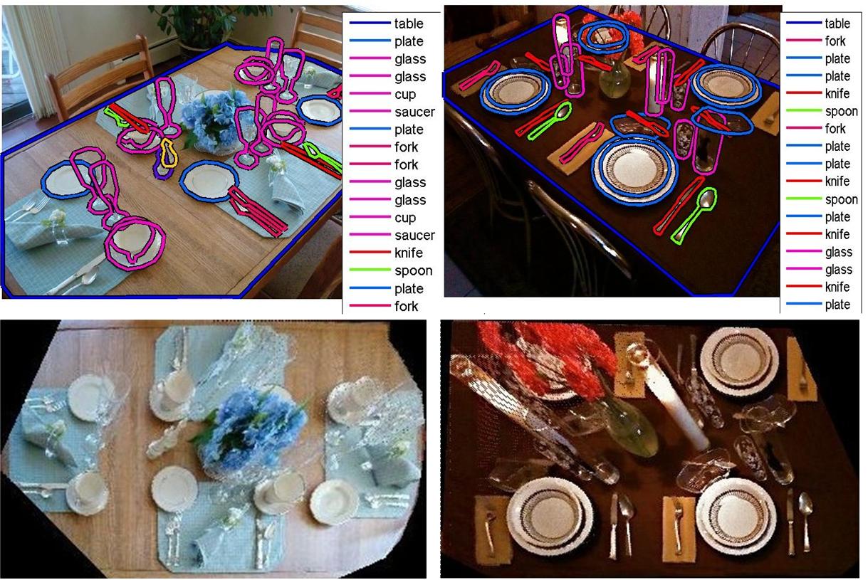
To estimate the homography (up to scale) at least four pairs of corresponding points are needed according to the Direct Linear Transformation (DLT) algorithm (Hartley and Zisserman, 2004, p. 88). These four pairs of corresponding points were located in the image coordinate system by annotators’ best visual judgment about four corners of a square in real world whose center coincides with the origin of the table (world) coordinate system. We are able to undo the projective distortion due to the perspective effect by back-projecting the table surface in the image coordinate system onto the world coordinate system. The homography matrices are scaled appropriately (using object’s typical sizes in real world) such that after back-projection the distance of object instances in the world coordinate system (measured in meters) can be computed. Figure 13 shows two typical images from this dataset and their rectified versions. Clearly, the main distortions occur for objects which are out of the table plane.

Each object instance was annotated with an object category label plus an enclosing polygon. Then, an ellipse was fit to the vertices of the polygon to estimate the object’s shape and pose in the image plane. Figure 13 (left) shows an example annotated image; Figure 13 (middle) shows the corresponding back-projection of vertices of annotation polygons for plates (in red), glasses (in green), and utensils (in black). Note that non-planar objects (e.g., glass) often get distorted after back projection (e.g., elongated green ellipses) since the homography transformation is a perspective projection from points on the table surface to the camera’s image plane. Hence, we estimated the base of vertical objects (shown by black circles in the middle figure) to estimate their location in the table (world) coordinate system since the center of fitting ellipse to the back-projection of such objects’ annotation points is not a good estimate of their 3D location in the real world. Figure 13 (right) shows top-view visualization of the annotated scene in the left using top-view icons of the corresponding object instances for plates, glasses, and utensils (note that all utensil instances are shown by top-view knife icons).

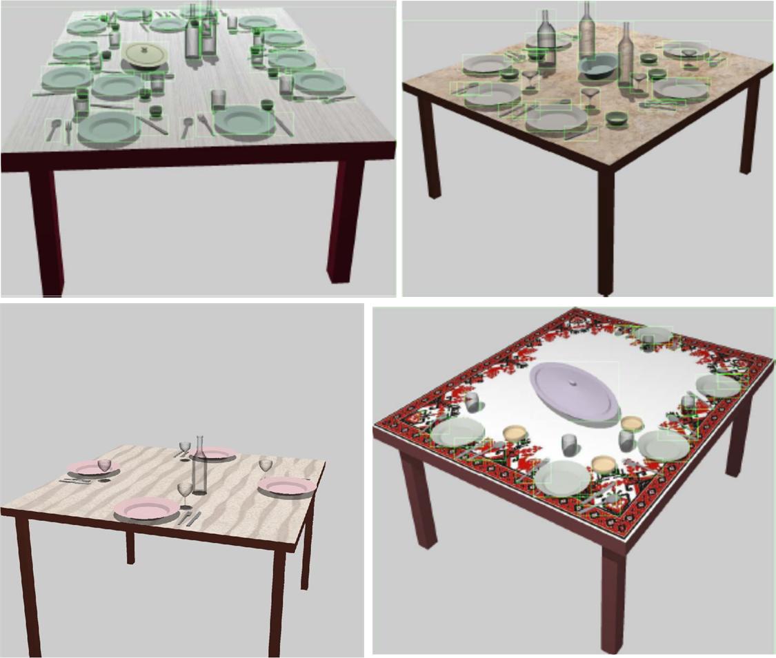
We also utilized a synthetic table-setting scene renderer for verification purposes. This synthetic image renderer inputs the camera’s calibration parameters, six rotation and translation camera’s extrinsic parameters, table length and width, and 3D object poses in the table’s coordinate system and outputs the corresponding table setting scene. Figure 14 shows some synthetic images generated by this renderer.

Figure 14: Synthetic table-setting scene samples.

10 Experiments and Results

10.1 Classifier Training

10.1.1 CatNet and ScaleNet

We fine-tuned CatNet using a set of 344,149 patches. The training set contained 170,830 patches from the “No Object” category, 36,429 patches from the “Plate” category, 2,074 patches from the “Bottle” category, 49,401 patches from the “Glass” category, and 85,415 patches from the “Utensil” category. If a patch includes multiple object instances, it is repeated in the training set, once for each instance. The train and test patches were extracted from the “JHU Table-Setting Dataset” using the image partitioning scheme explained in section 4.2. The “No Object” category patches were selected from the set of annocell patches whose overlap with the table area is less than $10\%$ of the patch. The number of such background training patches was chosen to be twice the number of patches from the most frequent category (utensil). We evaluated the performance of CatNet on a test set of 62,157 patches. Results from the raw output of CatNet are provided in Table 1, which shows the average scores in the vector of SoftMax scores returned by CatNet’s when it is applied to a patch from the corresponding class at different levels of the hierarchy. Unsurprisingly, for each category, the scores for that category increase as the patch size decreases (usually resulting in tighter patches to objects) when the category is present in the patch, which leads to higher classification accuracy being achieved for patches from finer levels of the annocell hierarchy.

Table 1: Average score at different levels of resolution of the annocell hierarchy when CatNet is applied to an input patch from the corresponding class.

Category	Level-0	Level-1	Level-2	Level-3
“No Object”	0.31	0.72	0.96	0.99
“Plate”	0.32	0.34	0.39	0.44
“Bottle”	0.08	0.19	0.31	0.36
“Glass”	0.33	0.44	0.56	0.68
“Utensil”	0.48	0.54	0.71	0.81

We fine-tuned ScaleNet on 171,395 patches. Each patch was labeled by one label $l\in\{1,2,3,4\}$, respectively associated to the closest scale ratios in $\{0.1,0.35,0.65,1\}$, the number of patches in each category being 42,567, 82,509, 37,443 and 8,876.

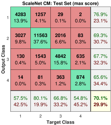
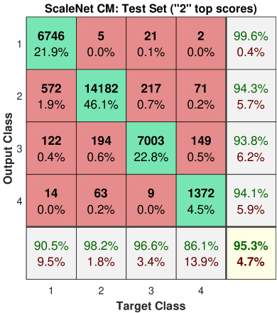
We evaluated the performance of ScaleNet on a test set of 30,742 patches. Figure 15 shows confusion matrices for test set in two cases of classification based on the maximum score class and top-2 score classes. A match is declared in the case of top-2 score classification if the true class is among the top two scores. It can be seen that the most common mistakes are made between consecutive classes which makes sense since consecutive classes are associated with consecutive scale ratios which have closer output distributions.

Figure 15: ScaleNet confusion matrix on “training” and “test” set considering both max score classification and top-2 classification.

Figure 16: CNN classifier detections for “plate”, “bottle”, and “glass”, and “utensil” categories from left to right. The ordinal numbers in brackets represent the confidence rank of detections per category and the fractional values in parentheses indicate the scale ratio of detections.

10.1.2 SceneNet

Figure 17: Table detection examples using TableNet: The fitting polygon, rectangle, and ellipse to the corner the points of patches at level–3 which were classified as table are shown in yellow, red, and magenta, respectively. The blue and green boxes show patches from, respectively, level-2 and level-3 classified as table. The estimated table size (in meters) based on each shape is shown on the green text boxes.

Figure 18: Noisy table detection examples using TableNet: The top row shows two examples with off-table false positives which were suppressed by considering the region with the maximum number of connected positive detections. The bottom row shows two poor table detection examples, perhaps due to the insufficient texture on the tables.

Figure 19: Histogram of the relative (left) and absolute (right) error made by the table–size estimator.

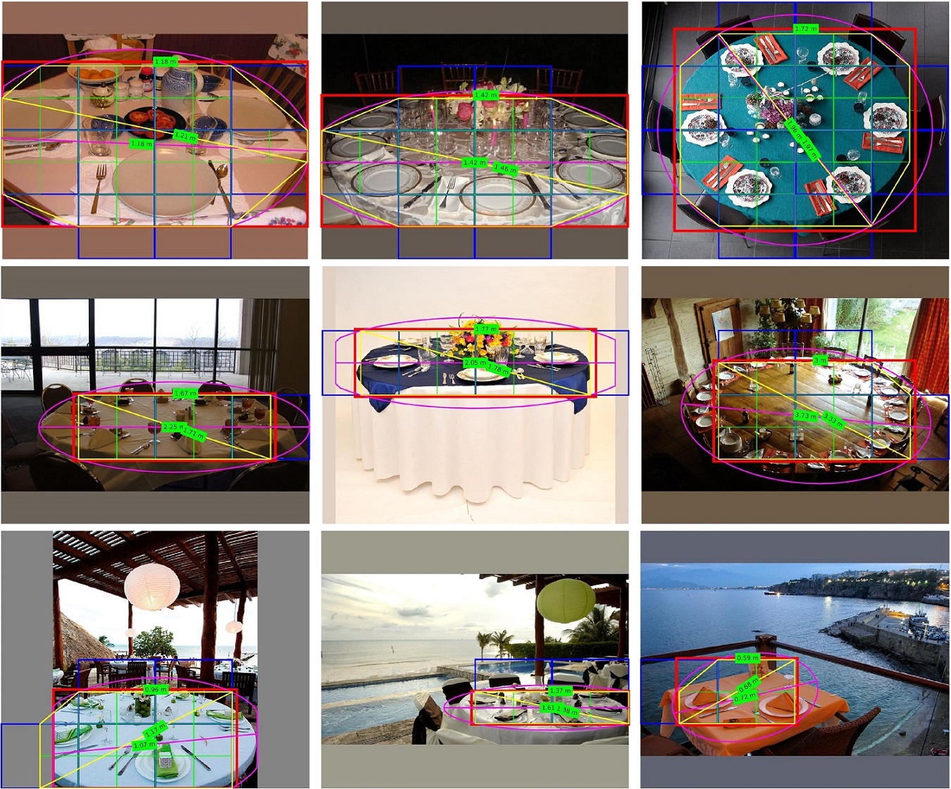
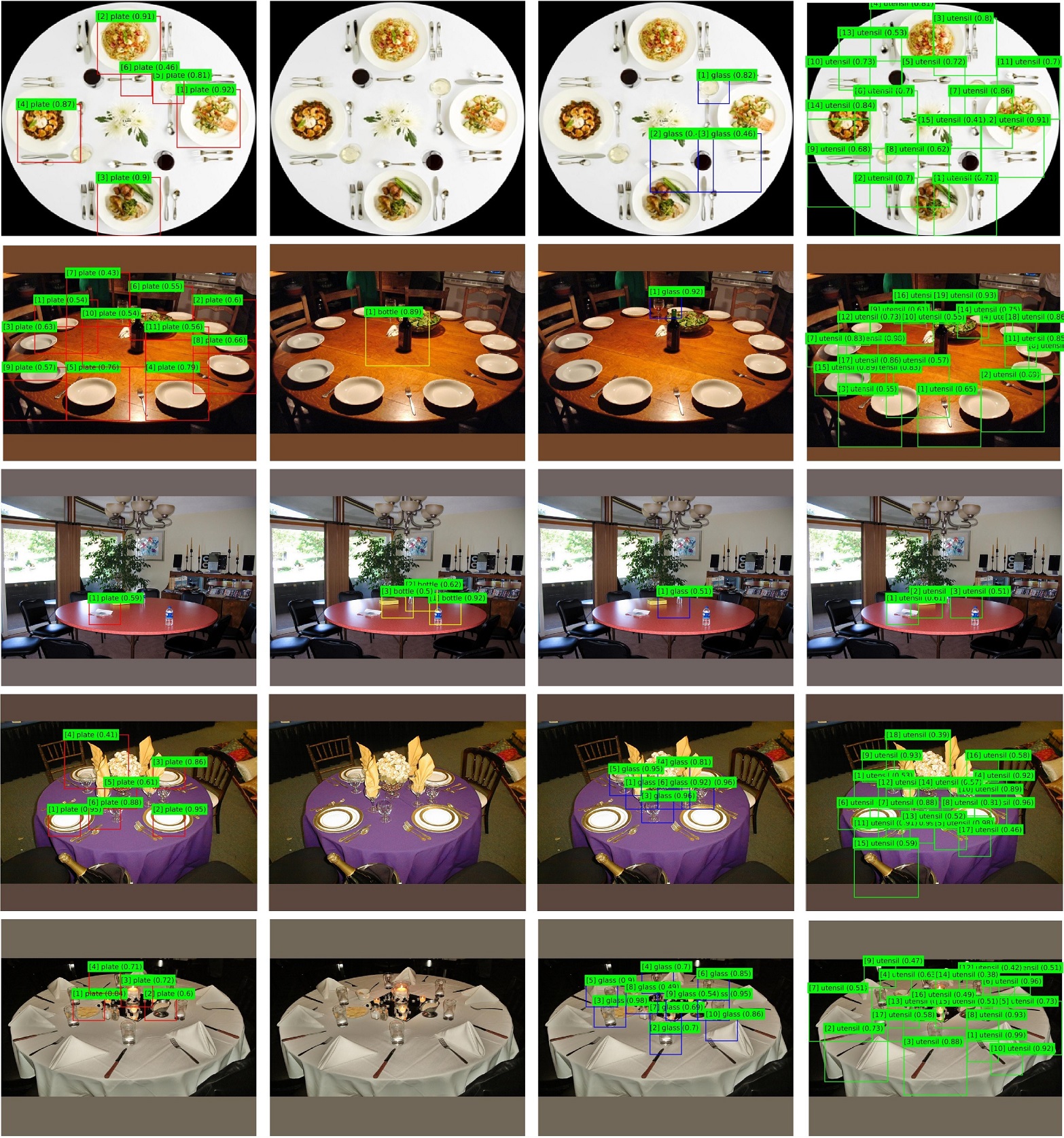
The main component of SceneNet is a CNN that detects whether a patch is part of the table area. We used 270,410 training patches (including 153,812 background and 116,598 table), and 38,651 test patches (including 18,888 background and 19,763 table). The background and table patches are defined by having, respectively, at most $10\%$ and at least $50\%$ (of the patch) overlap with the table surface area. All of the training and test patches were selected from level-2 and level-3 of the annocell hierarchy.

We classify a level-3 patch as part of the table if both its associated CNN and the one run on one of the level-2 patches that contain it report a positive detection. The final table area prediction, $\hat{M}$, is defined as the convex hull of the largest connected component of the union of detected level-3 patches. Figure 17 shows the estimated table area for some example images. Figure 18 (left and middle) shows two examples in which misdetected off-table patches are removed after post-processing. Figure 18 (right) shows a poor table detection example which seem to happen due to the lack of sufficient texture on the tables. We tested our table detector on 284 images and observed fewer than 5 poor table detections.

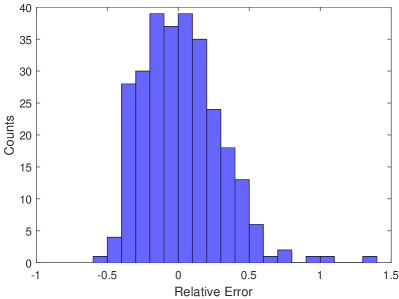
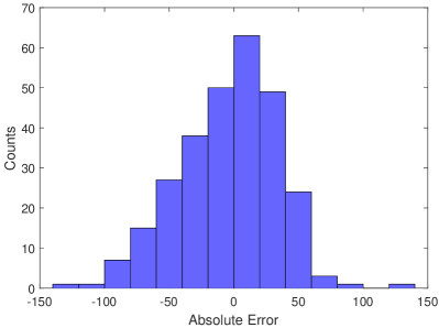
We estimate the table size (in 3D) by appropriately scaling the diameter length of its convex hall. The scale was calculated by running ScaleNet on patches from level 2 classified as table, and assuming that the table-setting objects have an average size of $20$cm. Figure 19 shows the histogram of the absolute and relative errors made by our table size estimator. We calculated the true table size by back-projecting the annotated table surface using the homography that was estimated from the annotation of the images. The histogram is centered roughly around 0 meaning that our table size estimator is relatively unbiased.

Figure 20: Questions at “early” IP steps.

Figure 21: Questions at “middle” IP steps.

Figure 22: Questions at “later” IP steps.

Figure 23: An example showing a plate instance not captured by annocells from the possibly best-fitting level (in green).

10.2 IP Experiments

Conditional inference on the posterior distribution $p(\xi|{\bf E}_{k})=P(Z=z,S=s,W=w|{\bf E}_{k})$ given the accumulated evidence after $k$ steps of IP, was described in section 7 (including, in particular, approximations made to the sampling of the scene geometry and camera properties). The templates we used for the geometry $S$ are square tables whose sizes range from 0.9 to 2.7 meters with 20cm intervals. We selected the template closest to the estimated table size and its two nearest neighbors (or one neighbor if the closest table size is 0.9 or 2.7). For each of them, we sampled 10 homographies which are consistent with the detected table surface area (described in section 10.1.2).

To generate homography samples that conform with the detected table area, assume a rectangular table with length $L_{s}$ and width $W_{s}$ whose four corner points are $(-L_{s}/2,-W_{s}/2)$, $(-L_{s}/2,W_{s}/2)$, $(L_{s}/2,-W_{s}/2)$, and $(L_{s}/2,W_{s}/2)$. We draw samples from the distribution on camera parameters $p(W)$ proposed in section 5.2 and calculate the corresponding homography matrix. Then, we project the four corners of the table to the image coordinate system using this homography matrix and check if the resulting polygon (quadrilateral) fits well to the detected table area using a similarity measure for 2D–shapes. We declare a “good fit” between two shapes $A_{1}$ and $A_{2}$ if their distance defined as $d(A_{1},A_{2})=|(A_{1}\cup A_{2})-(A_{1}\cap A_{2})|$ satisfies

$$d(A_{1},A_{2})<0.25\min(|A_{1}|,|A_{2}|).$$ (25)

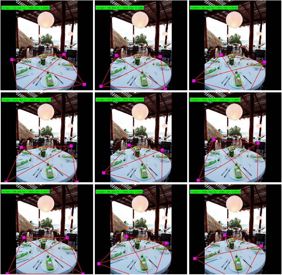
In an attempt to efficiently sample the homography (camera parameter) distribution that is consistent with the detected table area, we first try to find a set of camera parameters that result in a table projection meeting a relaxation of (25), namely $d(A_{1},A_{2})<0.4\hskip 1.42262pt\min(|A_{1}|,|A_{2}|)$, and as soon as we find such a sample we start to greedily fine–tune the camera parameters to finally satisfy (25). During fine-tuning we randomly choose one camera parameter and change it slightly by sampling a normal distribution with small variance centered at the previous value; we accept this change if it resulted in a smaller distance $d(A_{1},A_{2})$. We try a total of $10,000$ homographies obtained by sampling the camera model $p(W)$ (to satisfy the relaxed condition) or fine-tuning of parameters $W$ (to satisfy (25)) and exit the loop as soon as (25) is met; otherwise, if the condition (25) was not met during $10,000$ trials, we output the camera parameters resulting in the minimum $d(A_{1},A_{2})$. Figure 24 shows some example consistent homography samples.

Figure 24: Consistent homography samples satisfy condition (25).

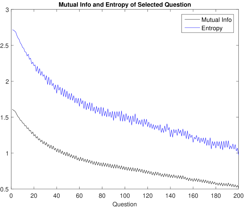
Recall that at step $k$, IP maximizes the mutual information $\mathcal{I}(X_{q},Y_{\mathcal{Q}}|\mathbf{E}_{k-1})$ over queries $q\in{\mathcal{Q}}$ and that this mutual information is the difference
$H(X_{q}|\mathbf{E}_{k-1})-{H}(X_{q}|Y_{\mathcal{Q}},\mathbf{E}_{k-1})$ (see (6)). Moreover, under our conditional independence assumptions, this reduces to the entropy of a mixture minus a mixture of entropies where in both cases the mixture weights are the conditional probabilities of the annobit $Y_{q}$ given the evidence. In the current case, the queries are indexed by the annocells $A\in{\mathcal{A}}$, where $Y^{cat}_{A}$ assumes sixteen possible values corresponding to the possible subsets of the four object categories. There are also scale annobits in correspondence with the classifiers $X^{sc}_{A}$ but we do not consider these in the selection of queries; of course each time we execute a CatNet classifier for an annocell $A$ we also execute the corresponding ScaleNet classifier for $A$ and both the CatNet and ScaleNet results are part of the evidence. Once the weights $P(Y^{cat}_{A}=y|{\bf E}_{k-1})$ are computed by sampling (see below) from the posterior, we can immediately evaluate the mixture of entropies since the entropy of the Dirichlet distribution has a closed-form solution. For the entropy of the mixture, namely the entropy of the mixture of $\sum_{y}Dir(X^{cat}_{A}|Y^{cat}_{A}=y)P(Y^{cat}_{A}=y|{\bf E}_{k-1})$ of Dirichlet densities, we estimate the integral by Monte Carlo integration. To generate a sample from the mixture distribution for the Monte Carlo integration, we first select one of the 16 Dirichlet densities with probabilities according to the posterior $P(Y^{cat}_{A}=y|{\bf E}_{k-1})$ and generate a sample from the selected Dirichlet distribution. Given generated samples from the mixture distribution we then evaluate negative logarithm of the mixture distribution at the generated samples and average to get an estimate of the entropy of the mixture. A similar approach can be taken to estimate the entropy of a Dirichlet distribution but since there is a closed-form solution for the entropy of Dirichlet distribution we used the closed-form solution in computing mixture of entropies. Nevertheless, by comparing the closed-form calculation of the Dirichlet distribution entropy and its Monte Carlo integration estimation we got insight about the appropriate number of mixture samples to reasonably estimate the entropy of mixture.

Turning back to the annobit posterior, we determine the states of the annobits from posterior samples $(\xi,s,w)$ by projecting the 3D samples $z$ to the image coordinate system using the sampled homography. More specifically, the projection of the sampled locations on the table plane in 3D obviously allows us to answer any queries about locations in the image plane appearing in the definition of an annobit. However, in order to determine what instances of objects are contained in a given annocell, and to measure the average sizes of the instances present, we need an estimate of the set of pixels which constitute the image realization of each instance sampled. For plates and utensils, which are effectively 2D, we simply use the projected circle for plates and projected ellipse for utensils, which of course are again ellipses in the image plane. For glasses and bottles, which are three-dimensional, we know the image representation is larger than the image ellipse obtained by projecting the base circle determined by the sample. Also, the projection of these objects in 2D is oriented perpendicular to the orientation of their base circle projection. Hence, we estimate the projection we would obtain for instances from these categories with a fully 3D to image mapping by moving the center of projection from the center of projected base upward (in the image) and along a vector orthogonal to the main axis of the projected base ellipse; we place the updated object center at a distance from the projected base center equal to half of its size where the size is proportional to the main diameter of the projected base.

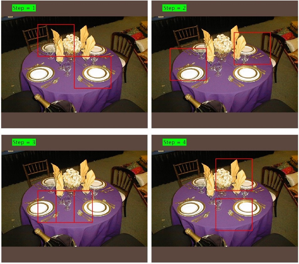
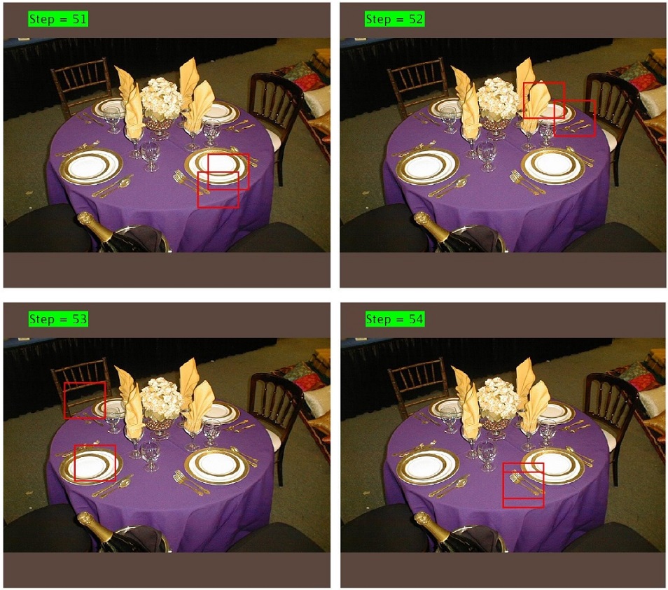
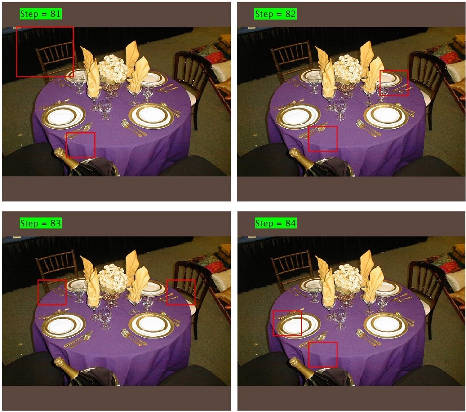
We ran IP on a dataset of 284 images. In each step of IP, two most informative questions corresponding to annobits with maximum mutual informations were asked, i.e., two patches were processed by CNNs. Figure 20 shows the annocells selected in the first four steps of IP for a given test image. Figure 21, 22 show the selected annocells at later IP steps. We can see that the patches selected later are usually from the finer levels which follows a coarse-to-fine scene analysis paradigm. However, it is completely plausible, and actually happened during our experiments, to go back again to a coarser question after asking a sequence of finer questions. Analogously, we as humans may focus on a particular area while analyzing a scene and then depending on the collected evidence can zoom out and collect evidence at a coarser level.

It is worthy to mention the difference between the IP selection criterion in (4) and the approximate criterion in (7) in terms of the resolution level of selected patches. According to our experiments, the approximate selection criterion in (7) usually starts with selecting coarser patches compared to the IP selection criterion in (4); more specifically the approximate criterion starts with level-1 whereas the exact criterion starts with level-2 (the reason of not starting with level-0, in the approximate criterion, is that in level-0, which is basically the whole image, most of categories exist. Therefore, analyzing the whole image will not result in much information gain if we are considering only one type of scene category). This is mainly due to the fact that the approximate criterion ignores the error rates of classifiers $X_{q}$ at the selection stage by replacing $X_{q}$ with $Y_{q}$. We know that our classifiers are more accurate at finer levels which leads to encouragement of their selection when using the IP criterion in (4). Note that in both criterions the questions selected at the early steps are usually coarser and they progressively refine (coarse-to-fine analysis). This is an interesting contrast between the two criterions. In support of the IP criterion in (4), assume Alice walks into a bookstore in Brooklyn, where Bob is the Bookstore clerk, in search for a novel that she does not remember its title. Bob wants to find the book that Alice is looking for by asking questions that are most informative to him and at the same time Alice can provide an answer to them. There is no point in asking a very informative question if Alice cannot provide an accurate answer to it e.g., Alice may be able to tell Bob what is the color of cover but most probably will not be able to mention the name of a few non-first characters in the novel. The IP selection criterion in (4) is trying to strike a tradeoff between the information gain of questions and the accuracy of the classifier at providing answer to them.

For the first 100 steps of IP, Figure 25 shows the maximal mutual information $\mathcal{I}(X^{cat}_{A_{k}},Y_{\mathcal{Q}}|\mathbf{E}_{k-1})$ for the selected annocell $A_{k}$ at step $k$, and the corresponding conditional entropy $H(Y^{cat}_{A_{k}}|\mathbf{E}_{k-1})$, both averaged across the 284 processed images. Hence $k=1,...,100$ but 200 classifiers are involved which explains the ripples with period two in this figure. This is because the second most informative question asked in each step usually has slightly lower conditional mutual information compared to the most informative question of the next step. Naturally the mutual information is smaller than the conditional entropy.

Figure 25: Mutual Information and Entropy of Selected Questions.

Figure 26: Precision-Recall Curves.

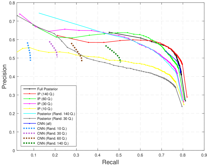
In order to define and visualize the detections generated by sampling from the 3D posterior distribution we superimpose a uniform grid of size $25\times 25$ on the image plane. We earlier explained how to associate a set of pixles with the projection of each sampled object instance, which in turn generates a rectangular bounding box. The center of the bounding box then falls into one of the above cells. For each cell and each category, we aggregate all samples from that category whose center lies in the cell and compute the average of the top-left corner and width/height of the corresponding bounding boxes; we take this average bounding box as the detection for that cell. The score for every detection is proportional to the number of 2D projections contributing to that detection (used to compute the average). We then run non-maximum suppression on the detections for each object category separately; two bounding boxes are considered neighbors if their intersection size over minimum size is greater than 0.3. This yields a final set of scored detections, each of which is labeled as a true positive if the intersection of the ground-truth bounding box and the estimated bounding box is at least 0.7 of the minimum of the two boxes and the ratio of their longest sides is between $0.5$ and $2$. Otherwise it is labeled a false positive.

10.3 Experiments with Stand-Alone Classifiers

In this section we consider parsing an image with the results of the classifiers alone, i.e., without the Bayesian model. For CatNet, from the softmax layer output, $X^{cat}_{A}$, we estimate the set of categories present in the annocell $A$ as follows. Let $S_{c}(A)$ denote the weight for category $c$ with input patch $A$. Order the weights, starting with the top one, then add new categories until the difference between the weights of the previous one and the new one is greater than a threshold $S_{g}=0.3$, or until three categories have been selected (including the “No Object” category).

For ScaleNet, from the output of $X^{sc}_{A}$ (a sequence of weights indexed by the scale categories), we compute an expected scale ratio $\widehat{SR}$ as a weighted average of the top two categories, i.e., letting $s,s^{\prime}$ be the top two categories with scores $w,w^{\prime}$, we take $\widehat{SR}=(ws+w^{\prime}s^{\prime})/(w+w^{\prime})$. We impose a selection criterion to declare an appropriate bounding box detection, ensuring in particular that objects present in the patch occupy a significant portion of it, by requiring that:

$$\widehat{SR}\geq 0.5-c\hat{\sigma}_{SR}$$ (26)

where $\hat{\sigma}_{SR}=\sqrt{(w^{2}+w^{\prime 2})/(w+w^{\prime})^{3}}|s-s^{\prime}|$ and $c=\sqrt{2\log 2}$. The choice made for $\hat{\sigma}_{SR}$ favors large differences between the top two scales. Note that ScaleNet returns the correct scale among its top two ratios more than 95% of the time when run on the test set. We also assign a score to the output of ScaleNet, namely $S_{scale}(A)=\exp(-\max(0,0.5-\widehat{SR})^{2}/2{\hat{\sigma}_{SR}}^{2})$.

Finally, each patch $A$ from the annocell hierarchy is given a mixed “Category–Scale” score per category. The mixed score for a given patch with scale score $S_{\text{scale}}(A)$ and the $c$-th category score $S_{c}(A)$ is $S_{c}(A)\times S_{\text{scale}}(A)$. We declare an annocell patch $A$ to be the bounding box of a positive detection for the $c$-th category if both $S_{\text{scale}}(A)\geq 0.5$ and $S_{c}(A)$ is among the CatNet’s top-3 scores with score gap $S_{g}=0.3$. We perform “non-maximum suppression” on the mixed scores of the positive detections per category to obtain a sparse set of boxes. Non-maximum suppression is performed by picking the most confident (maximum score) detection and removing its neighboring detections; then, picking the second most confident detection left and removing its neighbors, and continuing this process until there are no positive detections left. We consider two patches to be neighbors if at least $30\%$ of the smaller patch overlaps with the bigger patch (intersection over minimum greater than $0.3$).

It should be noted that an object instance may not necessarily fall completely inside any cell from our annocell hierarchy at a certain level even if there might exist a patch of the same size outside the hierarchy that completely includes that object instance. This is because the annocell hierarchy is constructed with $75\%$ overlap ($=25\%$ shift) between neighboring cells at the same level of resolution, and can therefore miss some object instances at a given level even if the cell size is large enough to include the object (e.g., see Figure 23). The only way to avoid this is to make the hierarchy exhaustive at each resolution, i.e., shifting patches by only one pixel at the time. Figure 16 illustrates some detection examples after running non-maximum suppression on the combined scores from the CatNet and ScaleNet.

10.4 Results

We generate PR-curves by thresholding the scores of surviving detections after non-maximum suppression. Note that we would like to detect as many true instances as possible (high recall) for as few mistakes as possible (high precision or low false detection rate) which invariably necessitates a trade-off. Figure 26 shows Precision–Recall curves for twelve different methods that we ran on the data set of 284 images for all object categories. According to Figure 26 the EP model-based detection performance improves as more classifiers are run and incorporated into the model. However, the full posterior detector seems to perform worse than information pursuit after 140 questions (after 70 IP steps with the batch size of 2) which seems counterintuitive because we expect to achieve better performance by incorporating more evidence. Note that by incorporating more classifiers we do not necessarily get better results due to the classifiers’ noise and increased likelihood of inconsistencies between the classifiers’ output. For example, consider Figure 27 where the 1st, 3rd, and 4th most confident plate detections (from CNN) are actually not a plate but the top or bottom of glasses; all of the annocells corresponding to these detections are from the finest level of the annocell hierarchy that are expected to be chosen later during the IP selection criterion and potentially degrade detection performance. Hence, integrating these classifiers would result in poorer inference due to the added classifiers inconsistency. Note that the model integrates the ScaleNet outputs in an attempt to suppress configurations with scale inconsistency (e.g., the incorrect plate detections in Figure 27). However, since a multiplication of CatNet and ScaleNet data model are used during posterior sampling (see (21) and consider the conditional independence assumption of CatNet and ScaleNet Dirichlet distributions), the model may not be able to completely suppress such configuration if the output of one of the CatNet or ScaleNet networks is large enough to compensate for the smaller one.

Figure 27: Confusing CNN detections example.

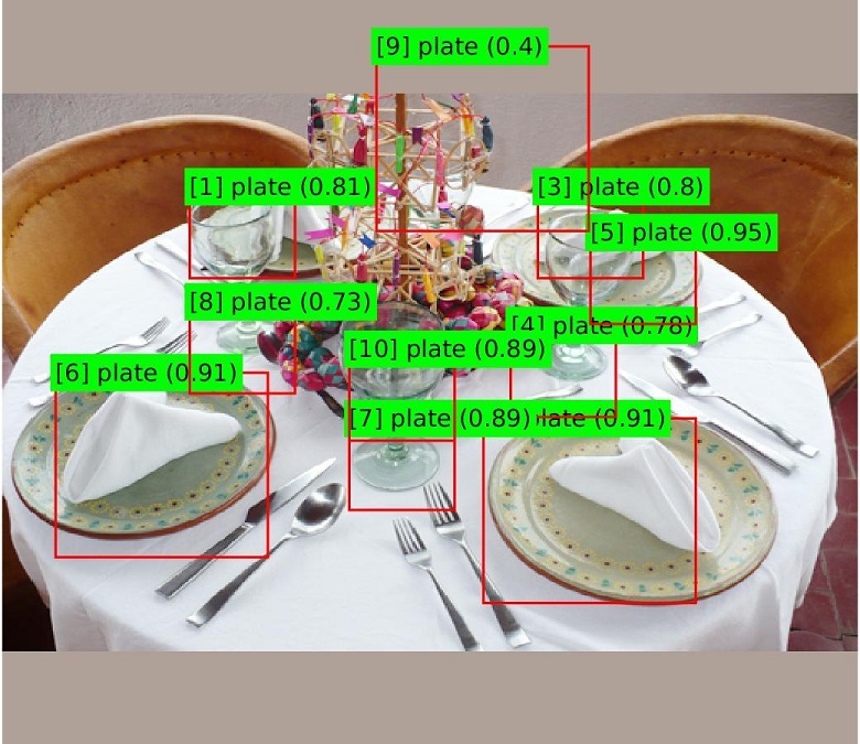
In Figure 26 we have included the P-R curves of model-based detection for two variations “Rand. 140 Q.” and “Rand. 30 Q.” with the same number of questions as in the two IP tests except that the questions are chosen at random; we have also included the result of CNN classifiers (no model) when 140, 60, 30, and 10 patches are randomly chosen and processed. One can see that the result with 140 randomly selected questions (the cyan curve in Figure 26) is almost the same as IP with only 30 questions asked (the magenta curve in Figure 26) which emphasizes the importance of efficient question selection in the Bayesian approach. The Bayesian approach provides a natural framework unifying the evidence collected from running tests and our prior knowledge encoding the contextual relations between different scene entities. Our experiments demonstrate that it makes significant difference to choose patches appropriately using our IP strategy versus randomly choosing them. In addition to saving the time it takes to process patches that do not provide much information, we can monitor the confidence of our detections (measured by conditional entropy) and stop processing more patches once the uncertainty saturates or starts to increase in case of conflicting evidence. The model-based approach with enough questions asked outperforms the CNN classifiers (higher precision at high recall area in the right). The result of running the CNN classifier on a small fraction of randomly selected annocells does not achieve high recall (see Figure 26).

Figure 28, 29, 30 show some qualitative model based detections based on full posterior, IP, and random selection of patches. One can see that detections based on IP outperform random selection for the same number of patches.

Figure 28: Detections based on full posterior, IP-140, IP-30, Rand-140, and Rand-30 (from top to bottom) for “plate”, “bottle”, and “glass”, and “utensil” categories (from left to right). The ordinal numbers in brackets represent the confidence rank of detections per category.

Figure 29: Detections based on full posterior, IP-140, IP-30, and Rand-30 (from top to bottom) for “plate”, “bottle”, and “glass”, and “utensil” categories (from left to right). The ordinal numbers in brackets represent the confidence rank of detections per category.

Figure 30: Detections based on full posterior, IP-140, IP-30, and Rand-30 (from top to bottom) for “plate”, “bottle”, and “glass”, and “utensil” categories (from left to right). The ordinal numbers in brackets represent the confidence rank of detections per category.

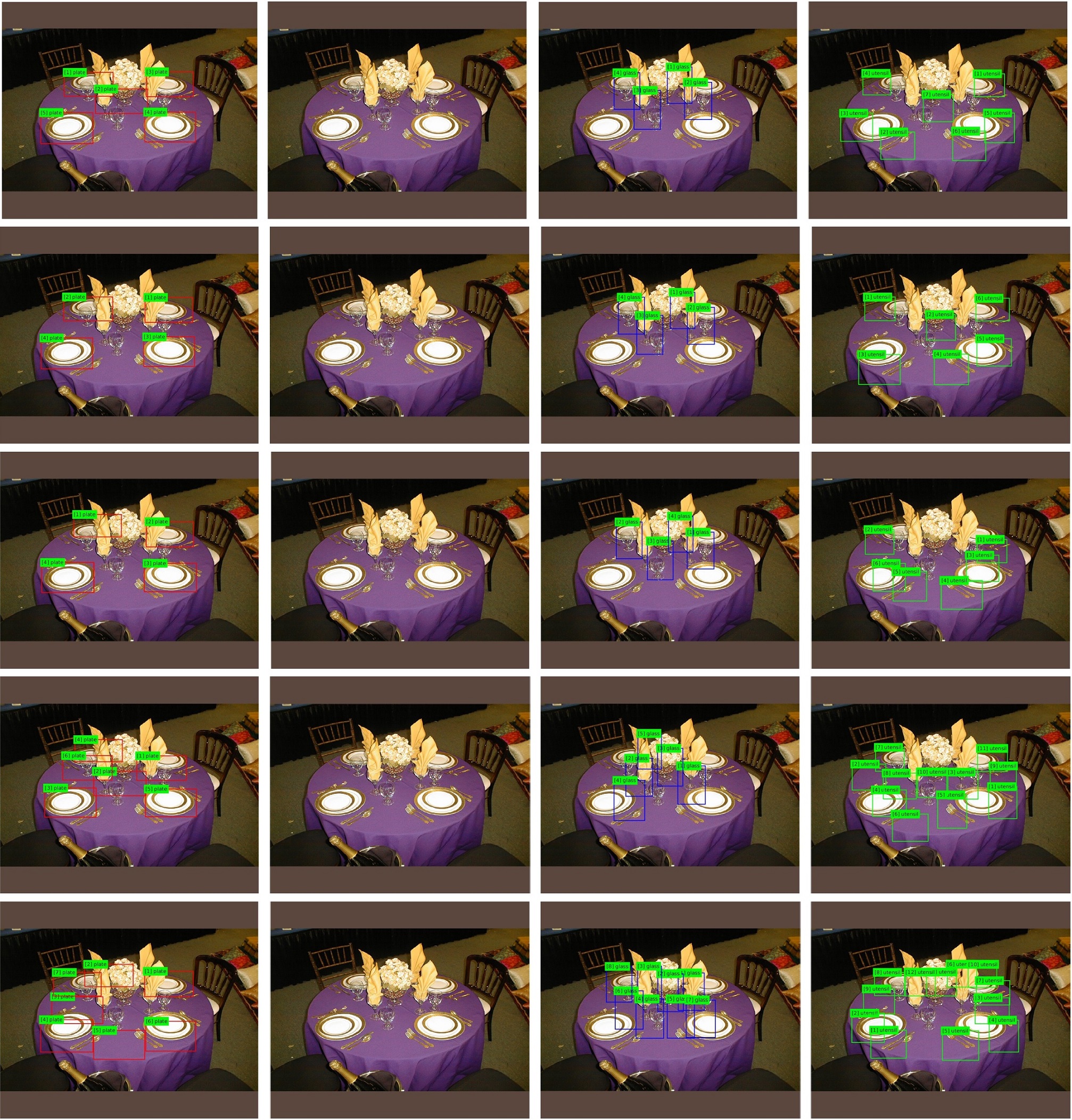
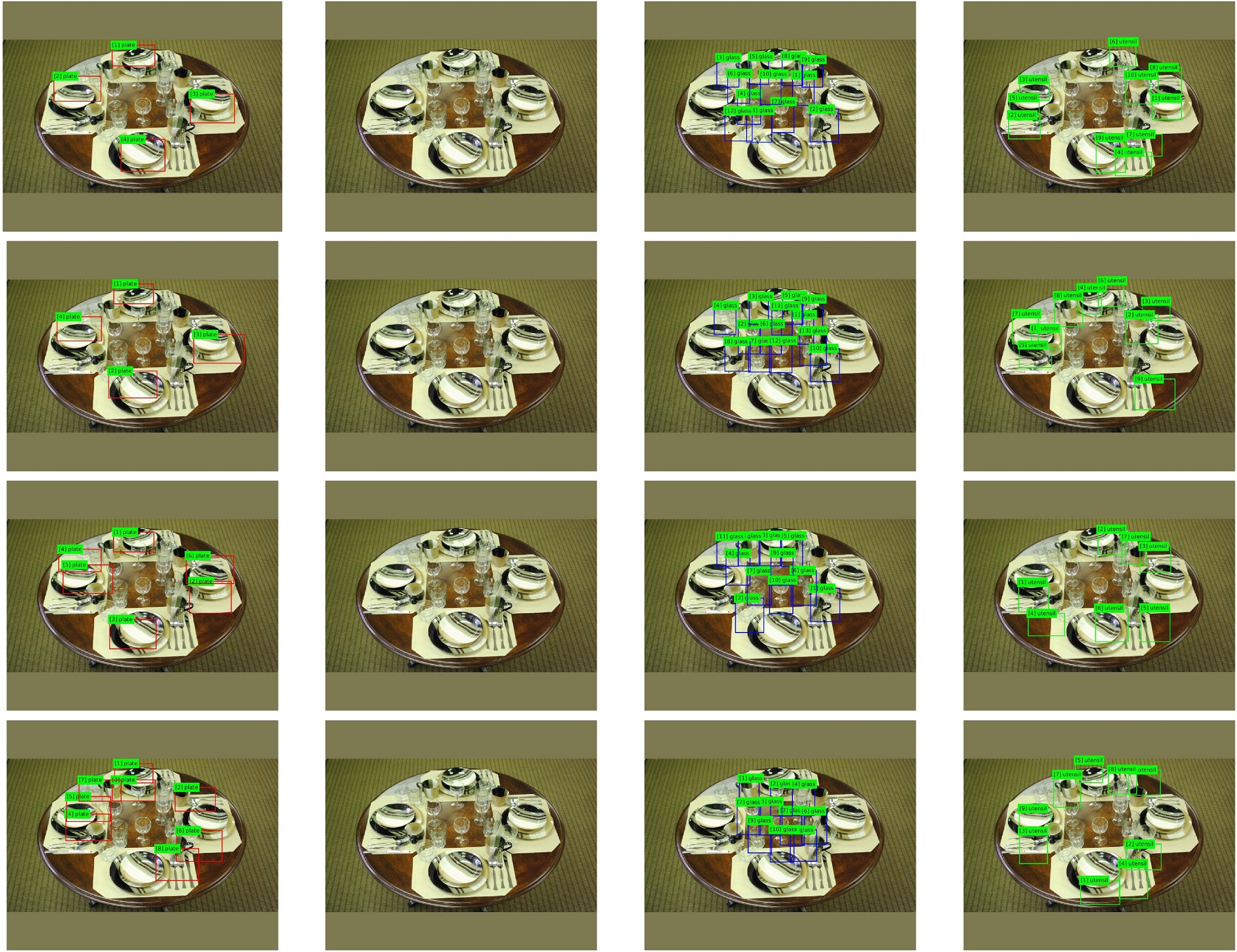
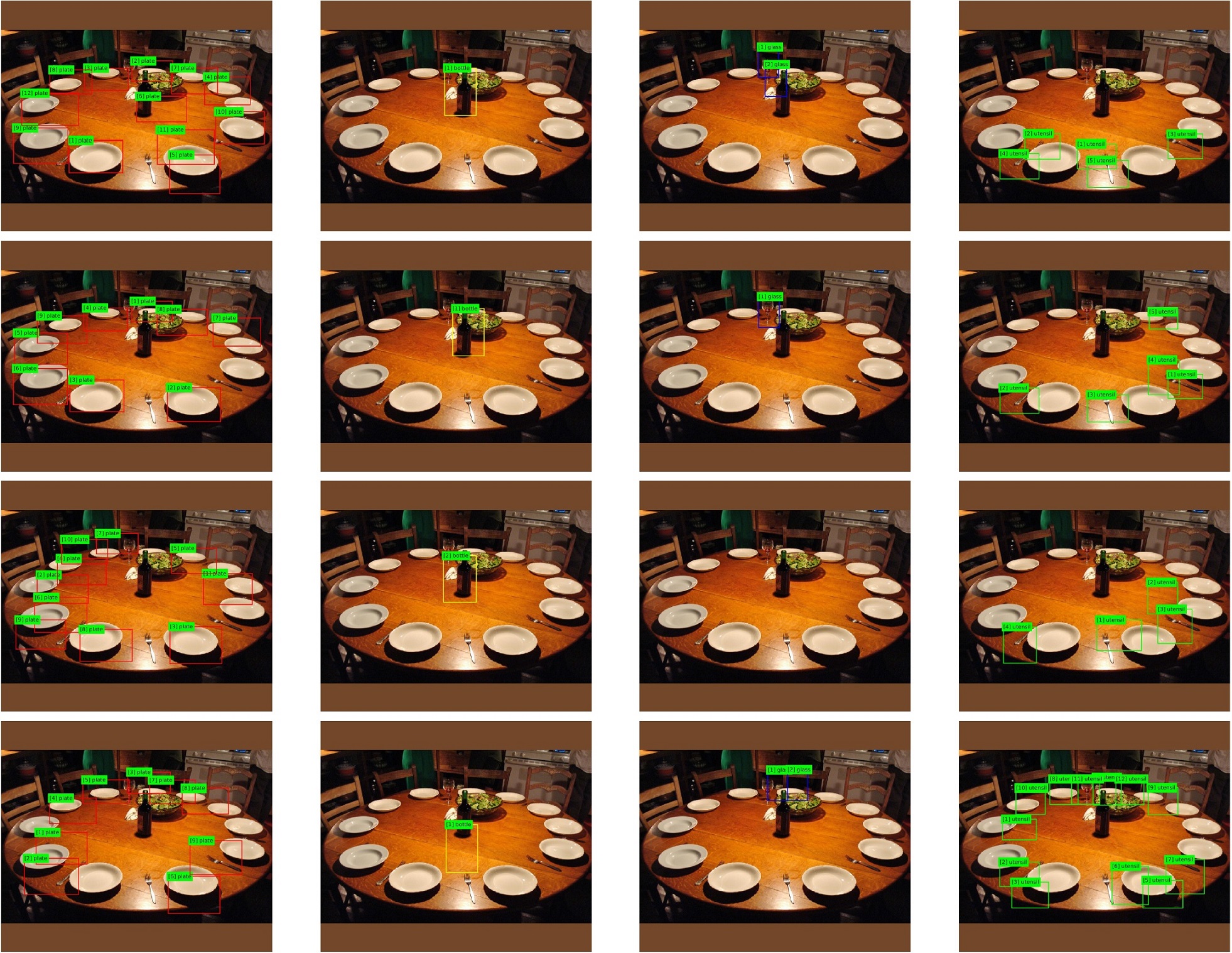
11 Conclusion

We proposed a new approach for multi-category object recognition, called “Information Pursuit” (IP), that sequentially investigates patches from an input test image in order to come up with an accurate description by processing as few patches as possible. Our approach follows the Bayesian framework with a prior model that incorporates the contextual relations between different scene entities such as the spatial and semantic relations among object instances, consistency of scales, constraints imposed by coplanarity of objects, etc. As proof of concept we applied the IP approach to table-setting scenes. We designed a novel generative model on attributed graphs with flexible structure where each node in the graph corresponds to an object instance attributed by its category label and 3D pose. This scene generation model model was not directly used in our IP framework, but the statistics calculated from its samples were used to learn a Markov Random Field (MRF) model employed directly by IP. Whereas, the scene generation model could be learned efficiently from the limited number of annotated images, the MRF model offered faster conditional inference. The entropy pursuit search strategy selects patches from the input image sequentially and investigates them to collect evidence about the scene. To investigate each patch we utilized state-of-the-art convolutional neural networks (CNNs). We introduced a new dataset of about 3000 fully annotated table-setting scenes to learn the scene generation model, to train a battery of CNN classifiers, and to test the performance of the IP algorithm. In summary, we studied the possibility of generating a scene interpretation by investigating only a fraction of all patches from an input image using the entropy pursuit Bayesian approach. The Bayesian framework is the natural approach for integrating contextual relations and the evidence collected using tests. We were able to show that by choosing the right patches in the right order we can identify an accurate interpretation by processing only a fraction of all patches from an input image.

Appendix

Appendix A Prior Distributions on Table Settings

We work with categories $\mathcal{C}=\{\text{plate},\text{bottle},\text{glass},\text{utensil}\}$ which are amongst the most annotated categories in our table-setting dataset. Instances from $\mathcal{C}$ are placed on a table whose geometric properties are denoted by $S$. In the simplified case that the table is rectangular we have $S=(L_{s},W_{s})$ where $L_{s}$ and $W_{s}$, respectively, represent the length and width of the table. We consider a world coordinate system whose origin is located at the center of the table’s surface, whose $z$ axis is orthogonal to the table’s surface, and assuming a rectangular table, the $x$ and $y$ axes are parallel to the edges of the table as illustrated in Figure 31. We also define a coordinate systems attached to the camera as shown in Figure 31.

Figure 31: Table and camera coordinate systems.

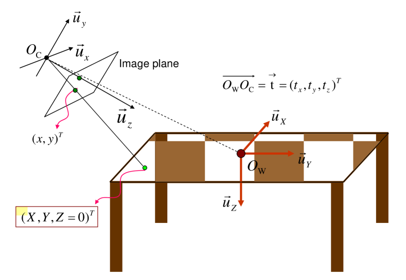
A.1 Attributed Graph Model

The general form of the attributed graph model is given by (19). We assume that given $S$ (and of course the scene type) the number of root nodes from different categories are independent:

$$p^{(0)}(\mathbf{n}|S)=\prod_{c\in\mathcal{C}}p^{(0)}_{c}(n_{c}|S),$$ (27)

where each of the univariate conditional distributions is modeled using a Poisson distribution with an average rate proportional to the scene area $A_{s}=L_{s}W_{s}$, so that

$$p^{(0)}_{c}(n_{c}|S)=e^{-\alpha_{c}A_{s}}\frac{(\alpha_{c}A_{s})^{n_{c}}}{n_{c}!},$$

resulting in $|\mathcal{C}|=4$ parameters $\alpha_{c},c\in\mathcal{C}$. We also decouple the offspring counts, letting $ch_{M}(c)$ denote the children of category $c$ in the master graph.

$$p^{(c)}(\mathbf{n})=\prod_{c^{\prime}\in ch_{M}(c)}p^{(c)}_{c^{\prime}}(n_{c^{\prime}}).$$ (28)

These distributions are modeled non-parametrically between $0$ and $l_{c_{0},c}$ chosen as follows (following edges $c_{0}\rightarrow c$ of the master graph): $l_{\text{plate},\text{utensil}}=l_{\text{plate},\text{glass}}=l_{\text{utensil},\text{utensil}}=3$ and $l_{\text{bottle},\text{glass}}=4$. This means that for example we allow at most three utensils to be adopted by a plate instance.

We now describe the pose distributions, starting with the root (spontaneous) objects. For each category $c$, the table region is divided into two parts: a rectangular strip of width $d_{c}$ starting from the edges, and the remainder interior region. The object’s center is placed in the central region with probability $\rho_{c}$ and in the outer strip with probability $1-\rho_{c}$. Conditionally to this choice, the distribution is uniform within each area. Plates are represented by circles on the table (they are flat), glasses and bottles by ellipsoids with a vertical principal direction and rotation invariant around this axis. Utensils are represented as horizontal ellipses (flat also), with orientation following a Von Mises distribution whose mean is set to be $90$ degrees from the orientation of the nearest table edge. The dispersion parameter of the von Mises distribution is set to zero if this instance is located farther than 40 centimeters from all sides of the table and greater than zero otherwise. Note that a von Mises distribution with zero dispersion parameter is basically a uniform distribution in $(0,2\pi]$. For simplicity, the object sizes are fixed (e.g., 25 centimeters for plate diameters).

We specify the pairwise pose distributions, $p^{(c)}(\theta|c_{0},\theta_{0},S)$, where $(c_{0},\theta_{0})$ is the category and pose of the parent object, by a radial distribution and a conditional angular distribution in a polar system centered at the location of the parent object. We model the relative pose of a parent-child object pair assuming that their relative location is independent from their relative orientation. We chose a scaled beta distribution for the radial distance between pairs of parent-child objects and either a von Mises (single or mixture) or uniform distribution for the angular location of the child in the periphery of the parent object. Normally, we expect a $c_{1}$-category parent and a $c_{2}$-category child to be within some distance from each other in order to justify their local contextual relationship. Let $d_{(c_{0},c)}$ denote this user-defined distance. The scale of the beta distribution used for the radial distance of a $(c_{0},c)$ object pair is set to $d_{(c_{0},c)}$ and kept fixed throughout design and learning. The set of pose distribution parameters therefore includes the set of beta and von Mises distributions’ parameters for different categories.

Appendix B Prior Distribution on Camera Rotation

The distribution of the rotation angles $\mathbf{\psi}$ is defined conditionally to translation $T$. Let $u_{x},u_{y},u_{z}$ denote the orthonormal axes for world coordinates, and $u_{x^{\prime}},u_{y^{\prime}},u_{z^{\prime}}$ the same axes for camera coordinates, the following constraints will be used: $u_{z^{\prime}}\sim-T/\|T\|$ (the camera points to the center of the table); $u_{x^{\prime}}\perp u_{z}$ (the horizontal direction in the image plane is nearly horizontal in 3D space); $u_{y^{\prime}}^{\top}u_{z}<0$ (the vertical direction in image plane points upward in 3D). Let

$$\bar{u}_{z^{\prime}}=-\frac{T}{\|T\|}$$

$$\bar{u}_{x^{\prime}}=\frac{\bar{u}_{z^{\prime}}\times u_{z}}{\|\bar{u}_{z^{\prime}}\times u_{z}\|}$$

$$\bar{u}_{y^{\prime}}=\bar{u}_{z^{\prime}}\times\bar{u}_{x^{\prime}}.$$

Letting $\boldsymbol{\mu}=(\mu_{x},\mu_{y},\mu_{z})$ denote the angle defining the rotation angles mapping $(u_{x},u_{y},u_{z})$ to $(\bar{u}_{x^{\prime}},\bar{u}_{y^{\prime}},\bar{u}_{z^{\prime}})$, we take $\psi_{x},\psi_{y},\psi_{z}$ conditionally independent given translation $T$, the marginals being von Mises distribution with means $\mu_{x},\mu_{y}$ and $\mu_{z}$. These angles are explicitly given by the formula

$$\mu_{y}=\sin^{-1}(-\bar{u}_{x^{\prime}}\cdot u_{z})$$

$$\mu_{x}=\measuredangle\left(\frac{\bar{u}_{z^{\prime}}\cdot u_{z}}{\cos\mu_{y}},\frac{\bar{u}_{y^{\prime}}\cdot u_{z}}{\cos\mu_{y}}\right)$$ (29)

$$\mu_{z}=\measuredangle\left(\frac{\bar{u}_{x^{\prime}}\cdot u_{x}}{\cos\mu_{y}},\frac{\bar{u}_{x^{\prime}}\cdot u_{y}}{\cos\mu_{y}}\right)$$

where $\measuredangle(a,b)$ is the angle $\theta$ defined by $\cos\theta=a$ and $\sin\theta=b$.

References

- Bao et al. (2010) Bao SY, Sun M, Savarese S (2010) “Toward Coherent Object Detection And Scene Layout Understanding”. In: CVPR
- Bengio et al. (2007) Bengio Y, Lamblin P, Popovici D, Larochelle H (2007) “Greedy Layer-Wise Training of Deep Networks”. In: Advances in Neural Information Processing Systems, MIT Press, pp 153–160
- Branson et al. (2014) Branson S, Van Horn G, Wah C, Perona P, Belongie S (2014) The ignorant led by the blind: A hybrid human–machine vision system for fine-grained categorization. International Journal of Computer Vision 108(1-2):3–29
- Celeux and Diebolt (1985) Celeux G, Diebolt J (1985) “The SEM Algorithm: A probabilistic teacher algorithm derived from the EM algorithm for the mixture problem”. Computational Statistics Quarterly 2:73–82
- Choi et al. (2012) Choi MJ, Torralba A, Willsky AS (2012) “A Tree-Based Context Model for Object Recognition”. IEEE Trans Pattern Anal Mach Intell 34(2):240–252
- Ciresan et al. (2011) Ciresan DC, Meier U, Masci J, Gambardella LM, Schmidhuber J (2011) “Flexible, High Performance Convolutional Neural Networks for Image Classification”. In: Proceedings of the Twenty-Second International Joint Conference on Artificial Intelligence, AAAI Press, IJCAI’11, vol 2, pp 1237–1242
- Dean et al. (2012) Dean J, Corrado G, Monga R, Chen K, Devin M, Mao M, Ranzato M, Senior A, Tucker P, Yang K, Le QV, Ng AY (2012) “Large Scale Distributed Deep Networks”. In: Advances in Neural Information Processing Systems, pp 1232–1240
- Dempster et al. (1977) Dempster AP, Laird NM, Rubin DB (1977) “Maximum likelihood from incomplete data via the EM algorithm”. J of the Royal Stat Soc Series B (Methodological) pp 1–38
- Deng et al. (2009) Deng J, Dong W, Socher R, Li LJ, Li K, Fei-Fei L (2009) “ImageNet: A Large-Scale Hierarchical Image Database”. In: CVPR09
- Deng et al. (2014) Deng J, Ding N, Jia Y, Frome A, Murphy K, Bengio S, Li Y, Neven H, Adam H (2014) “Large-Scale Object Classification using Label Relation Graphs”. In: ECCV
- Desai et al. (2011) Desai C, Ramanan D, Fowlkes C (2011) “Discriminative models for multi-class object layout”. Int J Comput Vision
- Felzenszwalb et al. (2010) Felzenszwalb PF, Girshick RB, McAllester D, Ramanan D (2010) “Object Detection with Discriminatively Trained Part-Based Models”. IEEE Trans Pattern Anal Mach Intell 32(9):1627–1645
- Geman and Jedynak (1996) Geman D, Jedynak B (1996) “An active testing model for tracking roads in satellite images”. IEEE Transactions on Pattern Analysis and Machine Intelligence 18(1):1–14
- Geman et al. (2015) Geman D, Geman S, Hallonquist N, Younes L (2015) Visual turing test for computer vision systems. Proceedings of the National Academy of Sciences 112(12):3618–3623
- Geman et al. (2002) Geman S, Potter DF, Chi Z (2002) “Composition systems”. Quarterly of Applied Mathematics pp 707–736
- Girshick et al. (2016) Girshick R, Donahue J, Darrell T, Malik J (2016) “Region-Based Convolutional Networks for Accurate Object Detection and Segmentation”. IEEE Transactions on Pattern Analysis and Machine Intelligence 38(1):142–158
- Hartley and Zisserman (2004) Hartley R, Zisserman A (2004) “Multiple View Geometry in Computer Vision”, 2nd edn. Cambridge
- Hastings (1970) Hastings WK (1970) “Monte Carlo sampling methods using Markov chains and their applications”. Biometrika 57(1):97–109
- Hinton et al. (2006) Hinton GE, Osindero S, Teh YW (2006) “A Fast Learning Algorithm for Deep Belief Nets”. Neural Comput 18(7):1527–1554
- Hoai and Zisserman (2014) Hoai M, Zisserman A (2014) “Talking Heads: Detecting Humans and Recognizing Their Interactions”. In: CVPR
- Hoiem and Savarese (2011) Hoiem D, Savarese S (2011) “Representations and Techniques for 3D Object Recognition and Scene Interpretation”. Synth. Lec. on Art. Int. and Mach. Learn., Morgan & Claypool Pub.
- Hoiem et al. (2007) Hoiem D, Efros AA, Hebert M (2007) “Recovering Surface Layout from an Image”. Int J Comput Vision 75(1):151–172
- Homma et al. (1988) Homma T, Atlas LE, Marks II RJ (1988) “An Artificial Neural Network for Spatio-Temporal Bipolar Patterns: Application to Phoneme Classification”. In: Neural Information Processing Systems, pp 31–40
- Jahangiri (2016) Jahangiri E (2016) On efficient bayesian scene interpretation. PhD thesis, Johns Hopkins University
- Jia et al. (2014) Jia Y, Shelhamer E, Donahue J, Karayev S, Long J, Girshick R, Guadarrama S, Darrell T (2014) “Caffe: Convolutional Architecture for Fast Feature Embedding”. arXiv preprint arXiv:14085093
- Lecun et al. (1998) Lecun Y, Bottou L, Bengio Y, Haffner P (1998) “Gradient-based learning applied to document recognition”. Proceedings of the IEEE 86(11):2278–2324
- Lee et al. (2010) Lee DC, Gupta A, Hebert M, Kanade T (2010) “Estimating Spatial Layout of Rooms using Volumetric Reasoning about Objects and Surfaces”. In: NIPS
- Liu et al. (2014) Liu X, Zhao Y, Zhu S (2014) “Single-View 3D Scene Parsing by Attributed Grammar”. In: CVPR
- Ma et al. (2003) Ma Y, Soatto S, Kosecka J, Sastry S (2003) An Invitation to 3D Vision: From Images to Geometric Models. Springer Verlag
- Metropolis et al. (1953) Metropolis N, Rosenbluth AW, Rosenbluth MN, Teller AH, Teller E (1953) “Equation of State Calculations by Fast Computing Machines”. Journal of Chemical Physics 21:1087–1092
- Minka (2012) Minka TP (2012) “The Fastfit Matlab toolbox”. http://research.microsoft.com/en-us/um/people/minka/software/fastfit/, [Online; accessed 15-Dec-2015]
- Mode (1971) Mode CJ (1971) “Multitype branching processes; theory and applications”. American Elsevier Pub. Co New York
- Mottaghi et al. (2014) Mottaghi R, Chen X, Liu X, Fidler S, Urtasun R, Yuille A (2014) “The Role of Context for Object Detection and Semantic Segmentation in the Wild”. In: CVPR
- Nemirovski et al. (2009) Nemirovski A, Juditsky A, Lan G, Shapiro A (2009) “Robust stochastic approximation approach to stochastic programming”. SIAM Journal on Optimization 19(4):1574–1609
- Porway et al. (2010) Porway J, Wang K, Zhu SC (2010) “A Hierarchical and Contextual Model for Aerial Image Understanding”. Int’l Journal of Computer Vision 88(2):254–283
- Rabinovich et al. (2007) Rabinovich A, Vedaldi A, Galleguillos C, Wiewiora E, Belongie S (2007) “Objects in context”. In: ICCV
- Ranzato et al. (2007) Ranzato M, Poultney C, Chopra S, LeCun Y (2007) “Efficient Learning of Sparse Representations with an Energy-Based Model”. In: Advances in Neural Information Processing Systems, MIT Press, pp 1137–1144
- Ren et al. (2015) Ren S, He K, Girshick R, Sun R (2015) Faster R-CNN: Towards real-time object detection with region proposal networks. In: Advances in Neural Information Processing Systems (NIPS)
- Reynolds et al. (1999) Reynolds JH, Chelazzi L, Desimone R (1999) “Competitive mechanisms subserve attention in macaque areas V2 and V4”. Journal of Neuroscience 19:1736–1753
- Roberts and Rosenthal (2001) Roberts GO, Rosenthal JS (2001) Optimal scaling for various Metropolis-Hastings algorithms. Statist Sci 16(4):351–367
- Russakovsky et al. (2015) Russakovsky O, Deng J, Su H, Krause J, Satheesh S, Ma S, Huang Z, Karpathy A, Khosla A, Bernstein M, Berg AC, Fei-Fei L (2015) “ImageNet Large Scale Visual Recognition Challenge”. International Journal of Computer Vision (IJCV) 115(3):211–252, DOI 10.1007/s11263-015-0816-y
- Russell et al. (2008) Russell BC, Torralba A, Murphy KP, Freeman WT (2008) “LabelMe: A Database and Web-Based Tool for Image Annotation”. Int J Comput Vision 77(1-3):157–173
- Saxena et al. (2009) Saxena A, Sun M, Ng AY (2009) “Make3D: Learning 3D Scene Structure from a Single Still Image”. IEEE Trans Pattern Anal Mach Intell 31(5):824–840
- Serences and Yantis (2006) Serences JT, Yantis S (2006) “Selective visual attention and perceptual coherence”. Trends in Cognitive Sciences 10(1):38–45, DOI http://dx.doi.org/10.1016/j.tics.2005.11.008
- Silberman et al. (2012) Silberman N, Hoiem D, Kohli P, Fergus R (2012) “Indoor Segmentation and Support Inference from RGBD Images”. In: ECCV
- Simonyan and Zisserman (2014) Simonyan K, Zisserman A (2014) “Very Deep Convolutional Networks for Large-Scale Image Recognition”. CoRR abs/1409.1556
- Sun et al. (2014) Sun M, Kim B, Kohli P, Savarese S (2014) “Relating Things and Stuff via ObjectProperty Interactions”. IEEE Trans Pattern Anal Mach Intell 36(7):1370–1383
- Sznitman and Jedynak (2010) Sznitman R, Jedynak B (2010) “Active Testing for Face Detection and Localization”. IEEE Transactions on Pattern Analysis and Machine Intelligence 32(10):1914–1920, DOI http://doi.ieeecomputersociety.org/10.1109/TPAMI.2010.106
- Sznitman et al. (2013) Sznitman R, Richa R, Taylor RH, Jedynak B, Hager GD (2013) “Unified Detection and Tracking of Instruments during Retinal Microsurgery”. IEEE Transactions on Pattern Analysis and Machine Intelligence 35(5):1263–1273
- Uijlings et al. (2013) Uijlings J, van de Sande K, Gevers T, Smeulders A (2013) “Selective Search for Object Recognition”. International Journal of Computer Vision
- Wei and Tanner (1990) Wei GCG, Tanner MA (1990) “A Monte Carlo Implementation of the EM Algorithm and the Poor Man’s Data Augmentation Algorithms”. Journal of the American Statistical Association 85(411):699–704