Robust Estimation of Change-Point Location

Abstract

We introduce a robust estimator of the location parameter for the change-point in the mean based on the Wilcoxon statistic and establish its consistency for $L_{1}$ near epoch dependent processes. It is shown that the consistency rate depends on the magnitude of change. A simulation study is performed to evaluate finite sample properties of the Wilcoxon-type estimator in standard cases, as well as under heavy-tailed distributions and disturbances by outliers, and to compare it with a CUSUM-type estimator. It shows that the Wilcoxon-type estimator is equivalent to the CUSUM-type estimator in standard cases, but outperforms the CUSUM-type estimator in presence of heavy tails or outliers in the data.

KEYWORDS: Wilcoxon statistic; change-point estimator; near epoch dependence Date: January 9, 2017.*Fakultät für Mathematik, Ruhr-Universität Bochum, 44780 Bochum, Germany

1 Introduction

In many applications it can not be assumed that observed data have a constant mean over time. Therefore, extensive research has been done in testing for change-points in the mean, see e.g. Giraitis et al. (1996), Csörgö and Horváth (1997), Ling (2007), and others. A number of papers deal with the problem of estimation of the change-point location. Bai (1994) estimates the unknown location point for the break in the mean of a linear process by the method of least squares. Antoch et al. (1995) and Csörgö and Horváth (1997) established the consistency rates for CUSUM-type estimators for independent data, while Csörgö and Horváth (1997) considered weakly dependent variables. Horváth and Kokoszka (1997) established consistency of CUSUM-type estimators of location of change-point for strongly dependent variables. Kokoszka and Leipus (1998, 2000) discussed CUSUM-type estimators for dependent observations and ARCH models. In spite of numerous studies on testing for changes and estimating for change-points, however, just a few procedures are robust against outliers in the data. In a recent work Dehling et al. (2015) address the robustness problem of testing for change-points by introducing a Wilcoxon-type test which is applicable under short-range dependence (see also Dehling et al. (2013) for the long-range dependence case).

In this paper we suggest a robust Wilcoxon-type estimator for the change-point location based on the idea of Dehling et al. (2015) and applicable for $L_{1}$ near epoch dependent processes. The Wilcoxon change-point test statistic is defined as

$$W_{n}(k)=\sum_{i=1}^{k}\sum_{j=k+1}^{n}(1_{\{X_{i}\leq X_{j}\}}-1/2)$$ (1)

and counts how often an observation of the second part of the sample, $X_{k+1},\ldots,X_{n}$, exceeds an observation of the first part, $X_{1},\ldots,X_{k}$. Assuming a change in mean happens at the time $k^{*}$, the absolute value of $W_{n}(k^{*})$ is expected to be large. Hence, the Wilcoxon-type estimator for the location of the change-point,

$$\hat{k}=\min\Big{\{}k:\max_{1\leq l<n}\Big{|}W_{n}(l)\Big{|}=\Big{|}W_{n}(k)\Big{|}\Big{\}},$$ (2)

can be defined as the smallest k for which the Wilcoxon test statistic $W_{n}(k)$ attains its maximum. Since the Wilcoxon test statistic is a rank-type statistic, outliers in the observed data can not affect the test statistic significantly. On the contrary, the CUSUM-type test statistic

$$C_{n}(k)=\frac{1}{k}\sum_{i=1}^{k}X_{i}-\frac{1}{n}\sum_{i=1}^{n}X_{i},$$

which compares the difference of the sample mean of the first $k$ observations and the sample mean over all observations, can be significantly disturbed by a single outlier.

The outline of the paper is as follows. In Section 2 we discuss the consistency and the rates of the estimator $\hat{k}$ in (2). Section 3 contains the simulation study. Section 4 provides useful properties of the Wilcoxon test statistic and the proof of the main result. Sections 5 and 6 contain some auxiliary results.

2 Definitions, assumptions and main results

Assume the random variables $X_{1},\ldots,X_{n}$ follow the change-point model

$$X_{i}=\begin{cases}Y_{i}+\mu,&1\leq i\leq k^{*}\\ Y_{i}+\mu+\Delta_{n},&k^{*}<i\leq n,\end{cases}$$ (3)

where the process $(Y_{j})$ is a stationary zero mean short-range dependent process, $k^{*}$ denotes the location of the unknown change-point and $\mu$ and $\mu+\Delta_{n}$ are the unknown means. We assume that $Y_{1}$ has a continuous distribution function $\operatorname{F}$ with bounded second derivative and that the distribution functions of $Y_{1}-Y_{k}$, $k\geq 1$ satisfy

$$\operatorname{P}(x\leq Y_{1}-Y_{k}\leq y)\leq C|y-x|,$$ (4)

for all $0\leq x\leq y\leq 1$, where $C$ does not depend on $k$ and $x,y$. We allow the magnitude of the change $\Delta_{n}$ vary with the sample size $n$.

Assumption 2.1.

1. The change-point $k^{*}=[n\theta]$, $0<\theta<1,$ is proportional to the sample size $n$.

2. The magnitude of change $\Delta_{n}$ depends on the sample size $n$, and is such that

   $$\Delta_{n}\rightarrow 0,\qquad n\Delta_{n}^{2}\rightarrow\infty,\qquad n\rightarrow\infty.$$ (5)

Next we specify the assumptions on the underlying process $(Y_{j})$. The following definition introduces the concept of an absolutely regular process which is also known as $\beta$-mixing.

Definition 2.1.

A stationary process $\left(Z_{j}\right)_{j\in\mathbb{Z}}$ is called absolutely regular if

$$\beta_{k}=\sup_{n\geq 1}\operatorname{E}\sup_{A\in\mathcal{F}_{1}^{n}}\left|\operatorname{P}\left(A|\mathcal{F}_{n+k}^{\infty}\right)-\operatorname{P}\left(A\right)\right|\rightarrow 0$$

as $k\rightarrow\infty$, where $\mathcal{F}_{a}^{b}$ is the $\sigma$-field generated by random variables $Z_{a},\ldots,Z_{b}$.

The coefficients $\beta_{k}$ are called mixing coefficients. For further information about mixing conditions see Bradley (2002). The concept of absolute regularity covers a wide range of processes. However, important processes like linear processes or AR processes might not be absolutely regular. To overcome this restriction, in this paper we discuss functionals of absolutely regular processes, i.e. instead of focusing on the absolute regular process $\left(Z_{j}\right)$ itself, we consider process $\left(Y_{j}\right)$ with $Y_{j}=f(Z_{j},Z_{j-1},Z_{j-2},\ldots)$, where $f:\mathbb{R}^{\mathbb{Z}}\rightarrow\mathbb{R}$ is a measurable function. The following near epoch dependence condition ensures that $Y_{j}$ mainly depends on the near past of $\left(Z_{j}\right)$.

Definition 2.2.

NED We say that stationary process $\left(Y_{j}\right)$ is $L_{1}$ near epoch dependent ($L_{1}$ NED) on a stationary process $\left(Z_{j}\right)$ with approximation constants $a_{k}$, $k\geq 0$, if conditional expectations $\operatorname{E}(Y_{1}|\mathcal{G}_{-k}^{k})$, where $\mathcal{G}_{-k}^{k}$ is the $\sigma$-field generated by $Z_{-k},\ldots,Z_{k}$, have property

$$\operatorname{E}\Big{|}Y_{1}-\operatorname{E}(Y_{1}|\mathcal{G}_{-k}^{k})\Big{|}\leq a_{k},\qquad k=0,1,2,\ldots$$

and $a_{k}\rightarrow 0$, $k\rightarrow\infty$.

Note that $L_{1}$ NED is a special case of more general $L_{r}$ near epoch dependence, where approximation constants are defined using $L_{r}$ norm: $\operatorname{E}\big{|}Y_{1}-\operatorname{E}(Y_{1}|\mathcal{G}_{-k}^{k})\big{|}^{r}\leq a_{k}$, $r\geq 1$. $L_{r}$ NED processes are also called $r$-approximating functionals. In testing problems considered in this paper we allow for heavy-tailed distributions. Hence, we deal with $L_{1}$ near epoch dependence, which assumes existence of only the first moment $\operatorname{E}|Y_{1}|$. The concept of near epoch dependence is applicable e.g. to GARCH(1,1) processes, see Hansen (1991), and linear processes, see example_linear_processes below. Borovkova et al. (2001) provide additional examples and information about properties of $L_{r}$ near epoch dependent process.

Example 2.1.

example_linear_processes Let $\left(Y_{j}\right)$ be a linear process, i.e. $Y_{t}=\sum_{j=0}^{\infty}\psi_{j}Z_{t-j}$, where $\left(Z_{j}\right)$ is white-noise process and the coefficients $\psi_{j}$, $j\geq 0$, are absolutely summable. Since $\left(Z_{j}\right)$ is stationary and $Z_{t-j}$ is $\mathcal{G}_{-k}^{k}$ measurable for $|t-j|\leq k$, we get

$$\operatorname{E}|Y_{t}-\operatorname{E}(Y_{t}|\mathcal{G}_{-k}^{k})|\leq\sum_{j=k+1}^{\infty}|\psi_{j}|\operatorname{E}|Z_{t-j}-\operatorname{E}(Z_{t-j}|\mathcal{G}_{-k}^{k})|\\ \leq 2\sum_{j=k+1}^{\infty}|\psi_{j}|\operatorname{E}|Z_{t-j}|=2\operatorname{E}|Z_{1}|\sum_{j=k+1}^{\infty}|\psi_{j}|.$$

Thus, the linear process $\left(Y_{j}\right)$ is $L_{1}$ NED on $\left(Z_{j}\right)$ with approximation constants $a_{k}=2\operatorname{E}|Z_{1}|\sum_{j=k+1}^{\infty}|\psi_{j}|$.

We will assume that the process $(Y_{j})$ in (3) is $L_{1}$ near epoch dependent on some absolutely regular process $\left(Z_{j}\right)$. In addition, we impose the following condition on the decay of the mixing coefficients $\beta_{k}$ and approximation constants $a_{k}$:

$$\sum_{k=1}^{\infty}{k^{2}\left(\beta_{k}+\sqrt{a_{k}}\right)}<\infty.$$ (6)

The next theorem states the rates of consistency of the Wilcoxon-type change-point estimator $\hat{k}$ given in (2) and the estimator $\hat{\theta}=\hat{k}/n$ of the true location parameter $\theta$ for the change-point $k^{*}=[n\theta]$.

Theorem 2.1.

consistence_of_bp_estimator Let $X_{1},\ldots,X_{n}$ follow the change-point model (3) and Assumption 2.1 be satisfied. Assume that $\left(Y_{j}\right)$ is a stationary zero mean $L_{1}$ near epoch dependent process on some absolutely regular process $\left(Z_{j}\right)$ and (6) holds. Then,

$$\Big{|}\hat{k}-k^{*}\Big{|}=O_{P}\Big{(}\frac{1}{\Delta_{n}^{2}}\Big{)},$$ (7)

and

$$\Big{|}\hat{\theta}-\theta\Big{|}=O_{P}\Big{(}\frac{1}{n\Delta_{n}^{2}}\Big{)}.$$ (8)

The rate of consistency of $\hat{\theta}$ in (8) is given by $n\Delta_{n}^{2}$. The assumption $n\Delta_{n}^{2}\rightarrow\infty$ in (5) implies $\hat{k}-k^{*}=o_{P}(k^{*})$ and yields consistency of the estimator: $\hat{\theta}\rightarrow_{p}\theta$. In particular, for $\Delta_{n}\geq n^{-1/2+\epsilon}$, $\epsilon>0$, the rate of consistency in (8) is $n^{2\epsilon}$: $\big{|}\hat{\theta}-\theta\big{|}=O_{P}\left(n^{-2\epsilon}\right)$.

The same consistency rate $n^{\epsilon}$ for the CUSUM-type change-point location estimator $\tilde{\theta}_{C}=\tilde{k}_{C}/n$, given by

$$\tilde{k}_{C}=\min\bigg{\{}k:\max_{1\leq i\leq n}\bigg{|}\sum_{j=1}^{i}X_{j}-\frac{i}{n}\sum_{j=1}^{n}X_{j}\bigg{|}=\bigg{|}\sum_{j=1}^{k}X_{j}-\frac{k}{n}\sum_{j=1}^{n}X_{j}\bigg{|}\bigg{\}},$$ (9)

was established by Antoch et al. (1995) for independent data and by Csörgö and Horváth (1997) for weakly dependent data.

3 Simulation results

In this simulation study we compare the finite sample properties of the Wilcoxon-type change-point estimator $\hat{k}$, given in (2), with the CUSUM-type estimator $\tilde{k}_{C}$, given in (9). We refer to the Wilcoxon-type change-point estimator by W and to the CUSUM-type estimator by C.

We generate the sample of random variables $X_{1},\ldots,X_{n}$ using the model

$$X_{i}=\begin{cases}Y_{i}+\mu&,1\leq i\leq k^{*}\\ Y_{i}+\mu+\Delta&,k^{*}<i\leq n\end{cases}$$ (10)

where $Y_{i}=\rho Y_{i-1}+\epsilon_{i}$ is an AR(1) process. In our simulations we consider $\rho=0.4$, which yields a moderate positive autocorrelation in $X_{i}$. The innovations $\epsilon_{i}$ are generated from a standard normal distribution and a Student’s t-distribution with 1 degree of freedom. We consider the time of change $k^{*}=[n\theta]$, $\theta=0.25,0.5,0.75$, the magnitude of change $\Delta=0.5,1,2$ and the sample sizes $n=50,100,200,500$. All simulation results are based on 10.000 replications. Note that we report estimation results not for $\hat{k}$ and $\tilde{k}_{C}$, but $\hat{\theta}=\hat{k}/n$ and $\tilde{\theta}_{C}=\tilde{k}_{C}/n$.

Figure 1 contains the histogram based on the sample of 10.000 values of Wilcoxon-type estimator $\hat{\theta}$ and the CUSUM-type estimator $\tilde{\theta}_{C}$, for the model (10) with $\Delta=1$, $\theta=0.5$, $n=50$ and independent standard normal innovations $\epsilon_{i}$. Both estimation methods give very similar histograms.

Table 1 reports the sample mean and the sample standard deviation based on 10.000 values of $\hat{\theta}$ and $\tilde{\theta}_{C}$ for other choices of parameters $\Delta$ and $\theta$. It shows that performance of both estimators improves when the sample size $n$ and the magnitude of change $\Delta$ are rising, and when the change happens in the middle of the sample. In general, Wilcoxon-type estimator performs in all experiments as good as the CUSUM-type estimator.

Figure 2 shows the histogram based on 10.000 values of $\hat{\theta}$ and $\tilde{\theta}_{C}$, for the model (10) with $t_{1}$-distributed heavy-tailed iid innovations $\epsilon_{i}$, $\Delta=1$, $\theta=0.5$ and $n=500$. For heavy-tailed innovations $\epsilon_{i}$, both estimators deviate from the true value of the parameter $\theta$ more significantly than under normal innovations. Nevertheless, the Wilcoxon-type estimator seems to outperform the CUSUM-type estimator.

Figure 3 shows the histogram based on 10.000 values for $\hat{\theta}$ and $\tilde{\theta}_{C}$ when the data $X_{1},\ldots,X_{n}$ is generated by (10) with $\Delta=1$, $\theta=0.5$, $n=200$ and $\epsilon_{i}\sim\operatorname{NIID}(0,1)$ and contains outliers. The outliers are introduced by multiplying observations $X_{[0.2n]}$, $X_{[0.3n]}$, $X_{[0.6n]}$ and $X_{[0.8n]}$ by the constant $M=50$. The histogram shows that the Wilcoxon-type estimator is rarely affected by the outliers, whereas the CUSUM-type estimator suffers large distortions.

Table 2 reports the sample mean and the sample standard deviation based on 10.000 values of $\hat{\theta}$ and $\tilde{\theta}_{C}$ for $\Delta=1$ and $\theta=0.5$ for sample size $n=50,100,200,500$ in the case of the normal, normal with outliers and $t_{1}$-distributed innovations. Figures 1, 2 and 3 presents results for $n=50,200,500$.

In general, we conclude that the Wilcoxon-type change-point location estimator performs equally well as the CUSUM-type change-point estimator in standard situations, but outperforms the CUSUM-type estimator in presence of heavy tails and outliers.

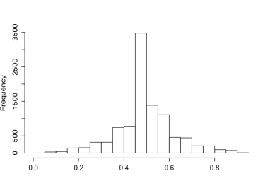
(a) CUSUM $\tilde{\theta}_{C}$

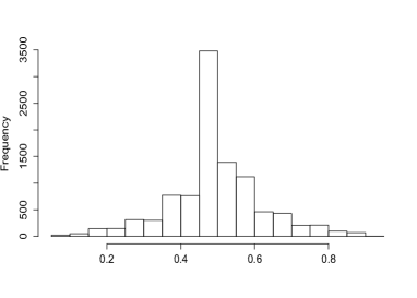
(b) Wilcoxon $\hat{\theta}$

Figure 1: Histogram based on 10.000 values for the Wilcoxon-type estimator $\hat{\theta}$ and the CUSUM-type estimator $\tilde{\theta}_{C}$. $X_{i}$ follows the model (10) with $\Delta=1$, $\theta=0.5$, $n=50$ and normal innovations $\epsilon_{i}\sim\operatorname{NIID}(0,1)$.

			n=50		n=100		n=200		n=500
$\Delta$	$\theta$		C	W	C	W	C	W	C	W
0.5	0.25	mean	0.46	0.46	0.43	0.44	0.40	0.40	0.34	0.34
		sd	0.21	0.21	0.20	0.20	0.18	0.18	0.13	0.13
	0.50	mean	0.50	0.50	0.50	0.50	0.50	0.50	0.50	0.50
		sd	0.18	0.18	0.16	0.16	0.13	0.13	0.08	0.08
	0.75	mean	0.54	0.54	0.57	0.56	0.61	0.61	0.66	0.66
		sd	0.20	0.20	0.20	0.20	0.18	0.18	0.13	0.13
1	0.25	mean	0.39	0.39	0.35	0.35	0.31	0.31	0.28	0.28
		sd	0.18	0.18	0.14	0.14	0.10	0.10	0.05	0.06
	0.50	mean	0.50	0.50	0.50	0.50	0.50	0.50	0.50	0.50
		sd	0.12	0.12	0.09	0.09	0.05	0.05	0.02	0.02
	0.75	mean	0.61	0.60	0.65	0.65	0.69	0.69	0.72	0.72
		sd	0.17	0.17	0.15	0.15	0.10	0.10	0.05	0.06
2	0.25	mean	0.30	0.31	0.28	0.29	0.27	0.28	0.26	0.26
		sd	0.10	0.10	0.06	0.07	0.04	0.04	0.02	0.02
	0.50	mean	0.50	0.50	0.50	0.50	0.50	0.50	0.50	0.50
		sd	0.05	0.05	0.03	0.03	0.02	0.01	0.01	0.01
	0.75	mean	0.69	0.68	0.72	0.71	0.73	0.73	0.74	0.74
		sd	0.09	0.10	0.06	0.07	0.04	0.04	0.02	0.02

Table 1: Sample mean and the sample standard deviation based on 10.000 values of $\hat{\theta}$ and $\tilde{\theta}_{C}$. $X_{i}$ follows the model (10) with normal innovations $\epsilon_{i}\sim\operatorname{NIID}(0,1)$.

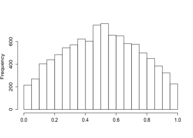
(a) CUSUM $\tilde{\theta}_{C}$

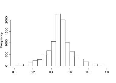
(b) Wilcoxon $\hat{\theta}$

Figure 2: Histogram of CUSUM-type estimator $\tilde{\theta}_{C}$ and Wilcoxon-type estimator $\hat{\theta}$ based on 10.000 values of $\tilde{\theta}_{C}$ and $\hat{\theta}$ for the model (10) with iid $t_{1}$-distributed innovations, $\Delta=1$, $\theta=0.5$ and $n=500$.

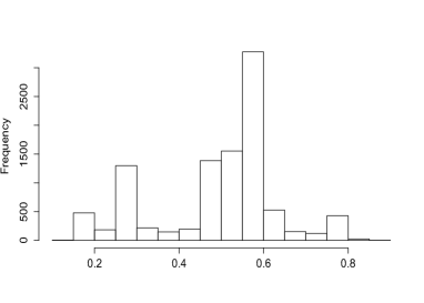
(a) CUSUM $\tilde{\theta}_{C}$

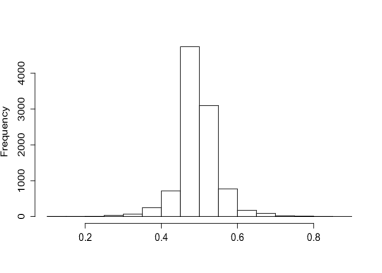
(b) Wilcoxon $\hat{\theta}$

Figure 3: Histogram based on 10.000 values of $\tilde{\theta}_{C}$ and $\hat{\theta}$ for the model (10) with normal innovations $\epsilon_{i}\sim\operatorname{NIID}(0,1)$, $\Delta=1$, $\theta=0.5$, $n=200$ and outliers.

		n=50		n=100		n=200		n=500
Innovations		C	W	C	W	C	W	C	W
normal	mean	0.50	0.50	0.50	0.50	0.50	0.50	0.50	0.50
	sd	0.12	0.12	0.09	0.09	0.05	0.05	0.02	0.02
$t_{1}$	mean	0.52	0.50	0.51	0.50	0.51	0.50	0.50	0.50
	sd	0.23	0.20	0.24	0.19	0.24	0.17	0.25	0.14
normal with	mean	0.50	0.49	0.50	0.50	0.50	0.50	0.51	0.50
outliers	sd	0.17	0.13	0.16	0.09	0.15	0.06	0.09	0.02

Table 2: Sample mean and the sample standard deviation of $\hat{\theta}$ and $\tilde{\theta}_{C}$ based on 10.000 replications for the normal, normal with outliers and $t_{1}$-distributed innovations, $\Delta=1$ and $\theta=0.5$.

4 Useful properties of the Wilcoxon test statistic and proof of consistence_of_bp_estimator

This section presents some useful properties of the Wilcoxon test statistic and the proof of consistence_of_bp_estimator.

Throughout the paper without loss of generality, we assume that $\mu=0$ and $\Delta_{n}>0$. We let $C$ denote a generic non-negative constant, which may vary from time to time. The notation $a_{n}\sim b_{n}$ means that two sequences $a_{n}$ and $b_{n}$ of real numbers have property $a_{n}/b_{n}\rightarrow c$, as $n\rightarrow\infty$, where $c\neq 0$ is a constant. $\|g\|_{\infty}=\sup_{x}|g(x)|$ stands for the supremum norm of function $g$. By $\xrightarrow{d}$ we denote the convergence in distribution, by $\rightarrow_{p}$ the convergence in probability and by $\overset{d}{=}$ we denote equality in distribution.

4.1 U-statistics and Hoeffding decomposition

The Wilcoxon test statistic $W_{n}(k)$ in (1) under the change-point model (3) can be decomposed into two terms

$$W_{n}(k)=\sum_{i=1}^{k}\sum_{j=k+1}^{n}(1_{\{X_{i}\leq X_{j}\}}-1/2)$$

$$=\begin{cases}\sum_{i=1}^{k}\sum_{j=k+1}^{n}(1_{\{Y_{i}\leq Y_{j}\}}-1/2)+\sum_{i=1}^{k}\sum_{j=k^{*}+1}^{n}1_{\{Y_{j}<Y_{i}\leq Y_{j}+\Delta_{n}\}},&1\leq k\leq k^{*}\\ \sum_{i=1}^{k}\sum_{j=k+1}^{n}(1_{\{Y_{i}\leq Y_{j}\}}-1/2)+\sum_{i=1}^{k^{*}}\sum_{j=k+1}^{n}1_{\{Y_{j}<Y_{i}\leq Y_{j}+\Delta_{n}\}},&k^{*}<k\leq n,\end{cases}$$

$$=\begin{cases}U_{n}(k)+U_{n}(k,k^{*}),&1\leq k\leq k^{*}\\ U_{n}(k)+U_{n}(k^{*},k),&k^{*}<k\leq n,\end{cases}$$ (11)

where

$$U_{n}(k) =\sum_{i=1}^{k}\sum_{j=k+1}^{n}(1_{\{Y_{i}\leq Y_{j}\}}-1/2), 1\leq k\leq n,$$ (12)

$$U_{n}(k,k^{*}) =\sum_{i=1}^{k}\sum_{j=k^{*}+1}^{n}1_{\{Y_{j}<Y_{i}\leq Y_{j}+\Delta_{n}\}}, 1\leq k\leq k^{*},$$ (13)

$$U_{n}(k^{*},k) =\sum_{i=1}^{k^{*}}\sum_{j=k+1}^{n}1_{\{Y_{j}<Y_{i}\leq Y_{j}+\Delta_{n}\}}, k^{*}<k\leq n.$$ (14)

The first term $U_{n}(k)$ depends only on the underlying process $(Y_{j})$, while the terms $U_{n}(k,k^{*})$ and $U_{n}(k^{*},k)$ depend in addition on the change-point time $k^{*}$ and the magnitude $\Delta_{n}$ of the change in the mean.

The term $U_{n}(k)$ can be written as a second order U-statistic

$$U_{n}\left(k\right)=\sum_{i=1}^{k}\sum_{j=k+1}^{n}\left(h\left(Y_{i},Y_{j}\right)-\Theta\right),\qquad 1\leq k\leq n,$$

with the kernel function $h\left(x,y\right)=1_{\left\{x\leq y\right\}}$ and the constant $\Theta=\operatorname{E}h\left(Y_{1}^{\prime},Y_{2}^{\prime}\right)=1/2$, where $Y_{1}^{\prime}$ and $Y_{2}^{\prime}$ are independent copies of $Y_{1}$.

We apply to $U_{n}\left(k\right)$ Hoeffding’s decomposition of U-statistics established by Hoeffding (1948). It allows to write the kernel function as the sum

$$h\left(x,y\right)=\Theta+h_{1}\left(x\right)+h_{2}\left(y\right)+g\left(x,y\right),$$ (15)

where

$$h_{1}\left(x\right) =\operatorname{E}h\left(x,Y_{2}^{\prime}\right)-\Theta=1/2-\operatorname{F}\left(x\right),\qquad h_{2}\left(y\right)=\operatorname{E}h\left(Y_{1}^{\prime},y\right)-\Theta=\operatorname{F}\left(y\right)-1/2,$$

$$g\left(x,y\right) =h\left(x,y\right)-h_{1}\left(x\right)-h_{2}\left(y\right)-\Theta.$$

By definition of $h_{1}$ and $h_{2}$, $\operatorname{E}h_{1}(Y_{1})=0$ and $\operatorname{E}h_{2}(Y_{1})=0$. Hence, $\operatorname{E}g(x,Y_{1})=\operatorname{E}g(Y_{1},y)=0$, i.e. $g(x,y)$ is a degenerate kernel.

The term $U_{n}(k,k^{*})$ in (13) (and $U_{n}(k^{*},k)$ in (14)) can be written as a U-statistic

$$U_{n}(k,k^{*})=\sum_{i=1}^{k}\sum_{j=k^{*}+1}^{n}h_{n}(Y_{i},Y_{j}),\qquad 1\leq k\leq k^{*},$$

with the kernel $h_{n}(x,y)=h(x,y+\Delta_{n})-h(x,y)=1_{\{y<x\leq y+\Delta_{n}\}}$. The Hoeffding decomposition allows to write the kernel as

$$h_{n}\left(x,y\right)=\Theta_{\Delta_{n}}+h_{1,n}\left(x\right)+h_{2,n}\left(y\right)+g_{n}\left(x,y\right),$$ (16)

with $\Theta_{\Delta_{n}}=\operatorname{E}1_{\{Y_{2}^{\prime}\leq Y_{1}^{\prime}\leq Y_{2}^{\prime}+\Delta_{n}\}},$

$$h_{1,n}\left(x\right) =\operatorname{E}h_{n}\left(x,Y_{2}^{\prime}\right)-\Theta_{\Delta_{n}}=\operatorname{F}\left(x\right)-\operatorname{F}\left(x-\Delta_{n}\right)-\Theta_{\Delta_{n}},$$

$$h_{2,n}\left(y\right) =\operatorname{E}h_{n}\left(Y_{1}^{\prime},y\right)-\Theta_{\Delta_{n}}=\operatorname{F}\left(y+\Delta_{n}\right)-\operatorname{F}\left(y\right)-\Theta_{\Delta_{n}},$$

$$g_{n}\left(x,y\right) =h_{n}\left(x,y\right)-h_{1,n}\left(x\right)-h_{2,n}\left(y\right)-\Theta_{\Delta_{n}}.$$

By assumption the distribution function $\operatorname{F}$ of $Y_{1}$ has bounded probability density $f$ and bounded second derivative. This allows to specify the asymptotic behaviour of $\Theta_{\Delta_{n}}$, as $n\rightarrow\infty,$

$$\Theta_{\Delta_{n}} =\operatorname{E}1_{\{Y_{2}^{\prime}<Y_{1}^{\prime}\leq Y_{2}^{\prime}+\Delta_{n}\}}=\operatorname{P}\left(Y_{2}^{\prime}<Y_{1}^{\prime}\leq Y_{2}^{\prime}+\Delta_{n}\right)$$

$$=\int_{\mathbb{R}}\left(\operatorname{F}\left(y+\Delta_{n}\right)-\operatorname{F}\left(y\right)\right)dF\left(y\right)=\Delta_{n}\bigg{(}\int_{\mathbb{R}}f^{2}\left(y\right)dy+o(1)\bigg{)}.$$ (17)

Note that $\operatorname{E}h_{1,n}(Y_{1})=0$ and $\operatorname{E}h_{2,n}(Y_{1})=0$. Therefore, $g_{n}(x,y)$ is a degenerate kernel, i.e. $\operatorname{E}g_{n}(x,Y_{1})=\operatorname{E}g_{n}(Y_{1},y)=0$. Furthermore, $\|h_{1,n}\|_{\infty}\rightarrow 0$, as $n\rightarrow\infty$, since

$$|h_{1,n}(x)|\leq|\operatorname{F}(x)-\operatorname{F}(x-\Delta_{n})-\Theta_{\Delta_{n}}|\leq C\Delta_{n}+\Theta_{\Delta_{n}}\leq C\Delta_{n},$$ (18)

where $C>0$ is a constant and $\Delta_{n}\rightarrow 0$, as $n\rightarrow\infty$.

4.2 1-continuity property of kernel functions $h$ and $h_{n}$

Asymptotic properties of near epoch dependent processes $(Y_{j})$ introduced in Section 2 are well investigated in the literature, see e.g. Borovkova et al. (2001). In the context of change-point estimation we are interested in asymptotic properties of the variables $h(Y_{i},Y_{j})$, where $h(x,y)=1_{\{x\leq y\}}$ is the Wilcoxon kernel, and also in properties of the terms $h_{1}(Y_{j})$ and $h_{1,n}(Y_{j})$ of the Hoeffding decomposition of the kernels in (15) and (16). We will need to show that the variables $(h(Y_{i},Y_{j}))$, $(h_{1}(Y_{j}))$ and $(h_{1,n}(Y_{j}))$ retain some properties of $(Y_{j})$. To derive them, we will use the fact that the kernels $h$ in (15) and $h_{n}$ in (16) satisfy the $1$-continuity condition introduced by Borovkova et al. (2001).

Definition 4.1.

1-continuous

We say that the kernel $h\left(x,y\right)$ is $1$-continuous with respect to a distribution of a stationary process $(Y_{j})$ if there exists a function $\phi(\epsilon)\geq 0$, $\epsilon\geq 0$ such that $\phi\left(\epsilon\right)\rightarrow 0$, $\epsilon\rightarrow 0$, and for all $\epsilon>0$ and $k\geq 1$

$$\operatorname{E}\left(\left|h\left(Y_{1},Y_{k}\right)-h\left(Y_{1}^{\prime},Y_{k}\right)\right|1_{\left\{\left|Y_{1}-Y_{1}^{\prime}\right|\leq\epsilon\right\}}\right) \leq\phi\left(\epsilon\right),$$ (19)

$$\operatorname{E}\left(\left|h\left(Y_{k},Y_{1}\right)-h\left(Y_{k},Y_{1}^{\prime}\right)\right|1_{\left\{\left|Y_{1}-Y_{1}^{\prime}\right|\leq\epsilon\right\}}\right) \leq\phi\left(\epsilon\right),$$

and

$$\operatorname{E}\left(\left|h\left(Y_{1},Y_{2}^{\prime}\right)-h\left(Y_{1}^{\prime},Y_{2}^{\prime}\right)\right|1_{\left\{\left|Y_{1}-Y_{1}^{\prime}\right|\leq\epsilon\right\}}\right) \leq\phi\left(\epsilon\right),$$ (20)

$$\operatorname{E}\left(\left|h\left(Y_{2}^{\prime},Y_{1}\right)-h\left(Y_{2}^{\prime},Y_{1}^{\prime}\right)\right|1_{\left\{\left|Y_{1}-Y_{1}^{\prime}\right|\leq\epsilon\right\}}\right) \leq\phi\left(\epsilon\right),$$

where $Y_{2}^{\prime}$ is an independent copy of $Y_{1}$ and $Y_{1}^{\prime}$ is any random variable that has the same distribution as $Y_{1}$.

For a univariate function $g(x)$ we define the $1$-continuity property as follows.

Definition 4.2.

The function $g\left(x\right)$ is $1$-continuous with respect to a distribution of a stationary process $(Y_{j})$ if there exists a function $\phi(\epsilon)\geq 0$, $\epsilon\geq 0$ such that $\phi\left(\epsilon\right)\rightarrow 0$, $\epsilon\rightarrow 0$, and for all $\epsilon>0$

$$\operatorname{E}\left(\left|g\left(Y_{1}\right)-g\left(Y_{1}^{\prime}\right)\right|1_{\left\{\left|Y_{1}-Y_{1}^{\prime}\right|\leq\epsilon\right\}}\right) \leq\phi\left(\epsilon\right),$$ (21)

where $Y_{1}^{\prime}$ is any random variable that has the same distribution as $Y_{1}$.

lemma_wilcoxon_1_continuous below establishes the $1$-continuity of functions $h(x,y)=1_{\{x\leq y\}}$ and $h_{n}(x,y)=1_{\{y<x\leq y+\Delta_{n}\}}$, $n\geq 1$. For $h_{n}$, $n\geq 1$ we assume that (19) and (20) hold with the same $\phi(\epsilon)$ for all $n\geq 1$. We start the proof by showing the $1$-continuity of the more general kernel function $h(x,y;t)=1_{\{x-y\leq t\}}$.

Lemma 4.1.

lemma_kernel:t_1_continuous Let $(Y_{j})$ be a stationary process, $Y_{1}$ have distribution function $F$ which has bounded first and second derivative and $Y_{1}-Y_{k}$, $k\geq 1$ satisfy (4). Then the function $h(x,y;t)=1_{\{x-y\leq t\}}$ is $1$-continuous with respect to the distribution function of $(Y_{j})$.

Proof.

The proof is similar to the proof of $1$-continuity of the kernel function $h(x,y;t)=1_{\{|x-y|\leq t\}}$ given in Example 2.2 of Borovkova et al. (2001).

Note that $1_{\{Y_{1}-Y_{k}\leq t\}}-1_{\{Y_{1}^{\prime}-Y_{k}\leq t\}}=0$ if $Y_{1}-Y_{k}\leq t$ and $Y_{1}^{\prime}-Y_{k}\leq t$; or $Y_{1}-Y_{k}>t$ and $Y_{1}^{\prime}-Y_{k}>t$. The difference is not zero if $Y_{1}-Y_{k}\leq t$ and $Y_{1}^{\prime}-Y_{k}>t$; or $Y_{1}-Y_{k}>t$ and $Y_{1}^{\prime}-Y_{k}\leq t$. Let $|Y_{1}-Y_{1}^{\prime}|\leq\epsilon$, where $\epsilon>0$. Then $Y_{1}-Y_{k}<t-\epsilon$ implies $Y_{1}^{\prime}-Y_{k}<t$, and $Y_{1}-Y_{k}>t+\epsilon$ implies $Y_{1}^{\prime}-Y_{k}>t$.

Hence, $|1_{\{Y_{1}-Y_{k}\leq t\}}-1_{\{Y_{1}^{\prime}-Y_{k}\leq t\}}|1_{\left\{\left|Y_{1}-Y_{1}^{\prime}\right|\leq\epsilon\right\}}\leq 1_{\left\{t-\epsilon\leq Y_{1}-Y_{k}\leq t+\epsilon\right\}}$. Therefore,

$$\operatorname{E}\left(\left|1_{\{Y_{1}-Y_{k}\leq t\}}-1_{\{Y_{1}^{\prime}-Y_{k}\leq t\}}\right|1_{\left\{\left|Y_{1}-Y_{1}^{\prime}\right|\leq\epsilon\right\}}\right)\leq\operatorname{P}\left(t-\epsilon\leq Y_{1}-Y_{k}\leq t+\epsilon\right)\leq C_{1}\epsilon,$$ (22)

because of assumption (4). Similar argument yields

$$\operatorname{E}\left(\left|1_{\{Y_{k}-Y_{1}\leq t\}}-1_{\{Y_{k}-Y_{1}^{\prime}\leq t\}}\right|1_{\left\{\left|Y_{1}-Y_{1}^{\prime}\right|\leq\epsilon\right\}}\right) \leq\operatorname{P}\left(t-\epsilon\leq Y_{1}-Y_{k}\leq t+\epsilon\right)\leq C_{1}\epsilon,$$

$$\operatorname{E}\left(\left|1_{\{Y_{1}-Y_{2}^{\prime}\leq t\}}-1_{\{Y_{1}^{\prime}-Y_{2}^{\prime}\leq t\}}\right|1_{\left\{\left|Y_{1}-Y_{1}^{\prime}\right|\leq\epsilon\right\}}\right) \leq\operatorname{P}(t-\epsilon\leq Y_{1}-Y_{2}^{\prime}\leq t+\epsilon)\leq C_{2}\epsilon,$$

$$\operatorname{E}\left(\left|1_{\{Y_{2}^{\prime}-Y_{1}\leq t\}}-1_{\{Y_{2}^{\prime}-Y_{1}^{\prime}\leq t\}}\right|1_{\left\{\left|Y_{1}-Y_{1}^{\prime}\right|\leq\epsilon\right\}}\right) \leq\operatorname{P}(t-\epsilon\leq Y_{1}-Y_{2}^{\prime}\leq t+\epsilon)\leq C_{2}\epsilon,$$

where $Y_{2}^{\prime}$ is an independent copy of $Y_{1}$, noting that by the mean value theorem and $|d\operatorname{F}(y)/dy|\leq C$,

$$\operatorname{P}(t-\epsilon\leq Y_{1}-Y_{2}^{\prime}\leq t+\epsilon) =\int_{\mathbb{R}}\left(\operatorname{F}\left(y+t+\epsilon\right)-\operatorname{F}\left(y+t-\epsilon\right)\right)dF\left(y\right)$$

$$\leq C\epsilon\int_{\mathbb{R}}f(y)dy=C_{2}\epsilon.$$

These bounds imply (19) and (20) with $\phi(\epsilon)=C\epsilon$, where $C$ does not depend on $t$. This completes the proof. ∎

Corollary 4.1.

lemma_wilcoxon_1_continuous Assume that assumptions of lemma_kernel:t_1_continuous are satisfied. Then,

1. Function $h(x,y)=1_{\{x\leq y\}}$ is $1$-continuous with respect to the distribution function of $(Y_{j})$.

2. Function $h_{n}(x,y)=1_{\{y<x\leq y+\Delta_{n}\}}$ is $1$-continuous with respect to the distribution function of $(Y_{j})$.

Proof.

(i) follows from lemma_kernel:t_1_continuous, noting that $1_{\{x\leq y\}}=h(x,y;0)$.

(ii) We need to verify (19) and (20). Write $h_{n}(x,y)=h(x,y)-h(x,y+\Delta_{n})=1_{\{x\leq y\}}-1_{\{x\leq y+\Delta_{n}\}}$. Then by (22),

$$\operatorname{E}\big{(}|h_{n}(Y_{1},Y_{k})-h_{n}(Y_{1}^{\prime},Y_{k})|1_{\left\{\left|Y_{1}-Y_{1}^{\prime}\right|\leq\epsilon\right\}}\big{)}\leq\operatorname{E}\big{(}|1_{\{Y_{1}\leq Y_{k}\}}-1_{\{Y_{1}^{\prime}\leq Y_{k}\}}|1_{\left\{\left|Y_{1}-Y_{1}^{\prime}\right|\leq\epsilon\right\}}\big{)}\\ +\operatorname{E}\big{(}|1_{\{Y_{1}\leq Y_{k}+\Delta_{n}\}}-1_{\{Y_{1}^{\prime}\leq Y_{k}+\Delta_{n}\}}|1_{\left\{\left|Y_{1}-Y_{1}^{\prime}\right|\leq\epsilon\right\}}\big{)}\leq C\epsilon.$$

Similar argument yields $\operatorname{E}\big{(}|h_{n}(Y_{k},Y_{1})-h_{n}(Y_{k},Y_{1}^{\prime})|1_{\left\{\left|Y_{1}-Y_{1}^{\prime}\right|\leq\epsilon\right\}}\big{)}\leq C\epsilon,$

$$\operatorname{E}\big{(}|h_{n}(Y_{1},Y_{2}^{\prime})-h_{n}(Y_{1}^{\prime},Y_{2}^{\prime})|1_{\left\{\left|Y_{1}-Y_{1}^{\prime}\right|\leq\epsilon\right\}}\big{)} \leq C\epsilon,$$

$$\operatorname{E}\big{(}|h_{n}(Y_{2}^{\prime},Y_{1})-h_{n}(Y_{2}^{\prime},Y_{1}^{\prime})|1_{\left\{\left|Y_{1}-Y_{1}^{\prime}\right|\leq\epsilon\right\}}\big{)} \leq C\epsilon.$$

Hence, (19) and (20) hold with $\phi(\epsilon)=C\epsilon$. ∎

Note that condition (4) is satisfied if variables $(Y_{1},Y_{k})$, $k\geq 1$, have joint probability densities that are bounded by the same constant $C$ for all $k$. If the joint density does not exist, for examples of verification of condition (4) see pages 4315, 4316 of Borovkova et al. (2001).

Lemma 2.15 of Borovkova et al. (2001) yields that if a general function $h(x,y)$ is $1$-continuous, i.e. satisfies (19) and (20) with function $\phi(\epsilon)$ then $\operatorname{E}h\left(x,Y_{2}^{\prime}\right)$, where $Y_{2}^{\prime}$ is an independent copy of $Y_{1}$, is also $1$-continuous and satisfies the condition in (21) with the same function $\phi(\epsilon)$. Hence, $h_{i}(x)$ and $h_{i,n}(x)$, $i=1,2$ are $1$-continuous and satisfy the condition in (21) with $\phi(\epsilon)=C\epsilon$.

Next we turn to $1$-continuity property of $g(x,y)$. By Hoeffding decomposition (15), $g(x,y)=h(x,y)-\Theta-h_{1}(x)-h_{2}(y)$. Since $h(x,y)$, $h_{1}(x)$ and $h_{2}(x)$ in (15) are $1$-continuous and satisfy (19), (20) and (21) with the same function $\phi(\epsilon)=C\epsilon$, then $g(x,y)$ is also $1$-continuous with function $\phi(\epsilon)=C\epsilon$. Indeed,

$$\operatorname{E}\left(|g(Y_{1},Y_{k})-g(Y_{1}^{\prime},Y_{k})|1_{\left\{\left|Y_{1}-Y_{1}^{\prime}\right|\leq\epsilon\right\}}\right)\\ \leq\operatorname{E}\left(|h(Y_{1},Y_{k})-h(Y_{1}^{\prime},Y_{k})|1_{\left\{\left|Y_{1}-Y_{1}^{\prime}\right|\leq\epsilon\right\}}\right)+\operatorname{E}\left(|h_{1}(Y_{1})-h_{1}(Y_{1}^{\prime})|1_{\left\{\left|Y_{1}-Y_{1}^{\prime}\right|\leq\epsilon\right\}}\right)\leq 2\phi(\epsilon)$$

and similarly, $\operatorname{E}\big{(}|g(Y_{k},Y_{1})-g(Y_{k},Y_{1}^{\prime})|1_{\left\{\left|Y_{1}-Y_{1}^{\prime}\right|\leq\epsilon\right\}}\big{)}\leq 2\phi(\epsilon)$.

Using the same argument, it follows that the function $g_{n}(x,y)=h_{n}(x,y)-\Theta_{\Delta_{n}}-h_{1,n}(x)-h_{2,n}(x)$ in the Hoeffding decomposition (16) is also $1$-continuous and satisfies (19), (20) with $\phi(\epsilon)=C\epsilon$.

4.3 NED property of $(h_{1}(Y_{j}))$ and $(h_{1,n}(Y_{j}))$

In Proposition 2.11 of Borovkova et al. (2001) it is shown that if $(Y_{j})$ is $L_{1}$ NED on a stationary absolutely regular process $(Z_{j})$ with approximation constants $a_{k}$ and $g(x)$ is $1$-continuous with function $\phi$, then $(g(Y_{j}))$ is also $L_{1}$ NED on $(Z_{j})$ with approximation constants $\phi\left(\sqrt{2a_{k}}\right)+2\sqrt{2a_{k}}||g||_{\infty}$.

Thus, the processes $(h_{1}(Y_{j}))$ and $(h_{2}(Y_{j}))$ in (15) and $(h_{1,n}(Y_{j}))$ and $(h_{2,n}(Y_{j}))$ in (16) are $L_{1}$ NED processes with approximation constants $a^{\prime}_{k}=C\sqrt{a_{k}}$.

Corollary 3.2 of Wooldridge and White (1988) provides a functional central limit theorem for partial sum process $\sum_{i=1}^{k}\tilde{Y}_{i}$, $k\geq 1$, where $(\tilde{Y}_{j})$ is $L_{2}$ NED on a strongly mixing process $(\tilde{Z}_{j})$. To apply this result to $(h_{1}(Y_{j}))$ which is $L_{1}$ NED on $(Z_{j})$ with approximation constants $a_{k}^{\prime}$, we need to show that $(h_{1}(Y_{j}))$ is also $L_{2}$ NED process. Note that the variables $\eta_{k}:=h_{1}(Y_{1})-\operatorname{E}(h_{1}(Y_{1})|\mathcal{G}_{-k}^{k})$ have property

$$\operatorname{E}\eta_{k}^{2}=\operatorname{E}\big{(}\eta_{k}^{2}1_{\big{\{}|\eta_{k}|\leq{a_{k}^{\prime}}^{-\frac{1}{2}}\big{\}}}\big{)}+\operatorname{E}\big{(}\eta_{k}^{2}1_{\big{\{}|\eta_{k}|>{a_{k}^{\prime}}^{-\frac{1}{2}}\big{\}}}\big{)}\\ \leq{a_{k}^{\prime}}^{-\frac{1}{2}}\operatorname{E}|\eta_{k}|+\sqrt{a_{k}^{\prime}}\operatorname{E}|\eta_{k}|^{4}\leq\sqrt{a_{k}^{\prime}}+\sqrt{a_{k}^{\prime}}C=:a_{k}^{\prime\prime}.$$

The last inequality holds, because by NED of $L_{1}$ near epoch dependence, $\operatorname{E}|h_{1}(Y_{1})-\operatorname{E}(h_{1}(Y_{1})|\mathcal{G}_{-k}^{k})|\leq a_{k}^{\prime}$ and because $|h_{1}(Y_{1})|\leq 1/2$. Therefore the process $(h_{1}(Y_{j}))$ is $L_{2}$ NED on $(Z_{j})$ with approximation constant $a_{k}^{\prime\prime}$. Since absolute regular process $(Z_{j})$ is strongly mixing process, from Corollary 3.2 of Wooldridge and White (1988), we obtain

$$\bigg{(}\frac{1}{n^{1/2}}\sum_{i=1}^{\left[nt\right]}h_{1}\left(Y_{i}\right)\bigg{)}_{0\leq t\leq 1}\xrightarrow{d}\left(\sigma W\left(t\right)\right)_{0\leq t\leq 1},$$

where $W\left(t\right)$ is a Brownian motion and $\sigma^{2}=\sum_{k=-\infty}^{\infty}\operatorname{Cov}(h_{1}(Y_{0}),h_{1}(Y_{k}))$.

Since $h_{2}(x)=-h_{1}(x)$, all properties of $(h_{1}(Y_{j}))$ remain valid also for $(h_{2}(Y_{j}))$.

4.4 Proof of consistence_of_bp_estimator

First we show consistency property $|k^{*}-\hat{k}|=o_{P}(k^{*})$ of the estimate $\hat{k}=\operatorname{argmax}_{1\leq k\leq n}|W_{n}(k)|$. To prove it, we verify that for any $\epsilon>0$,

$$\lim_{n\rightarrow\infty}\operatorname{P}\left(|k^{*}-\hat{k}|\leq\epsilon k^{*}\right)=1.$$ (23)

This means that the estimated value $\hat{k}$ with probability tending to $1$ is in a neighbourhood of the true value $k^{*}$:

$$\operatorname{P}\big{(}\hat{k}\in[k^{*}(1-\epsilon),k^{*}(1+\epsilon)]\big{)}\rightarrow 1.$$

We will show that as $n\rightarrow\infty$,

$$\operatorname{P}\Big{(}\max_{k:|k-k^{*}|\geq\epsilon k^{*}}|W_{n}(k)|<|W_{n}(k^{*})|\Big{)}\rightarrow 1.$$ (24)

Since $|W_{n}(k^{*})|\leq\max_{k:|k^{*}-k|\leq\epsilon k^{*}}|W_{n}(k)|$, this proves (23).

By (11),

$$W_{n}(k)=\begin{cases}U_{n}(k)+U_{n}(k,k^{*}),\qquad 1\leq k\leq k^{*}\\ U_{n}(k)+U_{n}(k^{*},k),\qquad k^{*}<k\leq n.\end{cases}$$

Theorem_DFGW implies $\max_{1\leq k\leq n}\left|U_{n}(k)\right|=O_{P}\left(n^{3/2}\right)$ and Lemma_abschaetzung_bp below yields

$$\max_{1\leq k\leq k^{*}}\left|U_{n}(k,k^{*})-k\left(n-k^{*}\right)\Theta_{\Delta_{n}}\right| =o_{P}\left(n^{3/2}\right),$$

$$\max_{k^{*}\leq k\leq n}\left|U_{n}(k^{*},k)-k^{*}\left(n-k\right)\Theta_{\Delta_{n}}\right| =o_{P}\left(n^{3/2}\right).$$

Hence,

$$W_{n}(k^{*}) =k^{*}(n-k^{*})\Theta_{\Delta_{n}}+(U_{n}(k^{*},k^{*})-k^{*}(n-k^{*})\Theta_{\Delta_{n}})+U_{n}(k^{*})$$

$$=k^{*}(n-k^{*})\Theta_{\Delta_{n}}+O_{P}(n^{3/2}),$$

$$\max_{1\leq k\leq k^{*}(1-\epsilon)}|W_{n}(k)| \leq(1-\epsilon)k^{*}(n-k^{*})\Theta_{\Delta_{n}}+O_{P}(n^{3/2}),$$

$$\max_{(1+\epsilon)k^{*}\leq k\leq n}|W_{n}(k)| \leq k^{*}(n-(1+\epsilon)k^{*})\Theta_{\Delta_{n}}+O_{P}(n^{3/2}).$$

Thus,

$$|W_{n}(k^{*})|-\max_{k:|k^{*}-k|\geq\epsilon k^{*}}|W_{n}(k)|\geq\epsilon\delta_{n}+O_{P}(n^{3/2}),$$

where $\delta_{n}=k^{*}\min(n-k^{*},{k^{*}})\Theta_{\Delta_{n}}$.

By definition $k^{*}=[n\theta]\sim n\theta$, and by (17) and (5), $\sqrt{n}\Theta_{\Delta_{n}}\sim c\sqrt{n}\Delta_{n}\rightarrow\infty$. Hence, $\delta_{n}^{-1}=o(n^{-3/2})$ and $\epsilon\delta_{n}+O_{P}(n^{3/2})=\epsilon\delta_{n}(1+O_{P}(n^{3/2}\delta_{n}^{-1}))=\epsilon\delta_{n}(1+o_{P}(1))$ which proves (24).

Next we establish the rate of convergence in (7), $k^{*}-k=O_{P}(1/\Delta_{n}^{2})$. Set $a(n)=\frac{M}{\Delta_{n}^{2}}$. Then for fixed $M>0$, $a(n)\rightarrow\infty$, as $n\rightarrow\infty$. We will verify that

$$\lim_{n\rightarrow\infty}\operatorname{P}\left(|k^{*}-\hat{k}|\leq a(n)\right)\rightarrow 1,\qquad\text{as}\;M\rightarrow\infty,$$

which implies (7). As in (24), we prove this by showing

$$\lim_{n\rightarrow\infty}\operatorname{P}\Big{(}\max_{k:|k-k^{*}|\geq a(n)}|W_{n}(k)|<|W_{n}(k^{*})|\Big{)}\rightarrow 1,\qquad\text{as}\;M\rightarrow\infty.$$ (25)

Define $V_{k}:=W_{n}^{2}\left(k\right)-W_{n}^{2}\left(k^{*}\right)$. If $|W_{n}\left(k\right)|$ attains its maximum at $k^{\prime}$, it is easy to see that $V_{k}$ attains its maximum at the same $k^{\prime}$. Hence, $\hat{k}=\min\{k:\max_{1\leq l\leq n}|W_{n}(l)|=|W_{n}(k)|\}=\min\{k:\max_{1\leq l\leq n}V_{l}=V_{k}\}$. Thus, instead of (25) it remains to show that

$$\lim_{n\rightarrow\infty}\operatorname{P}\Big{(}\max_{k:|k-k^{*}|\geq a(n)}V_{k}<0\Big{)}\rightarrow 1,\qquad M\rightarrow\infty.$$ (26)

Define $\tilde{k}:=\min\{k:|k-k^{*}|\leq\epsilon k^{*};V_{k}=\max_{n\alpha\leq l\leq n\beta}V_{l}\}$. Since by (23) $\hat{k}$ is a consistent estimator of $k^{*}$, it holds $\lim_{n\rightarrow\infty}\operatorname{P}(\hat{k}=\tilde{k})=1$.

So, in the proof of (26) it suffices to consider $\max$ over $k$, such that $|k-k^{*}|\leq\epsilon k^{*}$, $|k-k^{*}|\geq a(n)$, which corresponds to $(1-\epsilon)k^{*}\leq k\leq k^{*}-a(n)$ and $k^{*}+a(n)<k\leq(1+\epsilon)k^{*}$.

Let us start with $(1-\epsilon)k^{*}\leq k\leq k^{*}-a(n)$. Since $k^{*}-k>0$, relation (26) holds for such $k$, if

$$\lim_{n\rightarrow\infty}\operatorname{P}\Big{(}\max_{(1-\epsilon)k^{*}\leq k\leq k^{*}-a(n)}\frac{V_{k}}{(n(k^{*}-k))^{2}}<0\Big{)}\rightarrow 1,\qquad M\rightarrow\infty.$$ (27)

Note that

$$\frac{-V_{k}}{(n(k^{*}-k))^{2}} =\frac{W_{n}^{2}(k^{*})-W_{n}^{2}(k)}{(n(k^{*}-k))^{2}}$$

$$=-\bigg{(}\frac{W_{n}(k^{*})-W_{n}(k)}{n(k^{*}-k)}\bigg{)}^{2}+2\frac{W_{n}(k^{*})-W_{n}(k)}{n(k^{*}-k)}\frac{W_{n}(k^{*})}{n(k^{*}-k)}.$$ (28)

By (11), $W_{n}(k)=U_{n}(k)+U_{n}(k,k^{*})$. Then,

$$\frac{W_{n}(k^{*})-W_{n}(k)}{n(k^{*}-k)}=\frac{n-k^{*}}{n}\Theta_{\Delta_{n}}+\delta_{1,k}+\delta_{2,k},$$

where

$$\delta_{1,k}=\frac{U_{n}(k^{*})-U_{n}(k)}{n(k^{*}-k)},\qquad\delta_{2,k}=\frac{U_{n}(k^{*},k^{*})-U_{n}(k,k^{*})}{n(k^{*}-k)}-\frac{n-k^{*}}{n}\Theta_{\Delta_{n}}.$$

Observe that by (17), $\Theta_{\Delta_{n}}\sim c_{*}\Delta_{n}$, $c_{*}>0$, and $k^{*}/n\rightarrow\theta$. Therefore, $(n-k^{*})/n\Theta_{\Delta_{n}}\sim c_{0}\Delta_{n}$, where $c_{0}=(1-\theta)c_{*}$. Moreover, $\max_{1\leq k\leq k^{*}-a(n)}|\delta_{i,k}|=o_{P}(\Delta_{n})$, $i=1,2$, by (47) and (48) of Lemma_abschaetzung_gewichtetes_maximum. Hence,

$$\frac{W_{n}(k^{*})-W_{n}(k)}{n(k^{*}-k)}=c_{0}\Delta_{n}(1+o_{P}(1)),\qquad\bigg{(}\frac{W_{n}(k^{*})-W_{n}(k)}{n(k^{*}-k)}\bigg{)}^{2}=c_{0}^{2}\Delta_{n}^{2}(1+o_{P}(1)).$$ (29)

In turn,

$$\frac{W_{n}(k^{*})}{n(k^{*}-k)}=\frac{U_{n}(k^{*},k^{*})}{n(k^{*}-k)}+\frac{U_{n}(k^{*})}{n(k^{*}-k)}$$

and

$$\frac{U_{n}(k^{*},k^{*})}{n}=\frac{k^{*}(n-k^{*})\Theta_{\Delta_{n}}}{n}+\frac{\delta_{3,k}}{n},$$

where $\delta_{3,k}=U_{n}(k^{*},k^{*})-k^{*}(n-k^{*})\Theta_{\Delta_{n}}$. By Lemma_abschaetzung_bp, $\max_{1\leq k\leq k^{*}}\delta_{3,k}/n=o_{P}(n^{1/2})$. Since

$$\frac{k^{*}(n-k^{*})\Theta_{\Delta_{n}}}{n}\sim k^{*}c_{0}\Delta_{n}\sim\theta c_{0}n\Delta_{n}$$

and $\sqrt{n}=o(n\Delta_{n})$, this implies

$$\frac{U_{n}(k^{*},k^{*})}{n}=k^{*}c_{0}\Delta_{n}(1+o_{P}(1)).$$

Next, by Theorem_DFGW below, $U_{n}(k^{*})=O_{P}(n^{3/2})$, and hence, $U_{n}(k^{*})/n=O_{P}(n^{1/2})$. Therefore, $W_{n}(k^{*})/n=k^{*}c_{0}\Delta_{n}(1+o_{P}(1))$. Hence, for $(1-\epsilon)k^{*}\leq k\leq k^{*}-a(n)$,

$$\frac{W_{n}(k^{*})}{n(k^{*}-k)}=\frac{k^{*}c_{0}\Delta_{n}(1+o_{P}(1))}{k^{*}-k}\geq\frac{1}{\epsilon}c_{0}\Delta_{n}(1+o_{P}(1)).$$ (30)

Using (29) and (30) in (4.4), it follows

$$-\frac{V_{k}}{(n(k^{*}-k))^{2}}\geq\frac{2}{\epsilon}c_{0}^{2}\Delta_{n}^{2}(1+o_{P}(1))-c_{0}^{2}\Delta_{n}^{2}(1+o_{P}(1))\geq\Big{(}\frac{2}{\epsilon}-1\Big{)}(c_{0}\Delta_{n})^{2}(1+o_{P}(1))>0.$$

This proves (27). Similar argument yields

$$\lim_{n\rightarrow\infty}\operatorname{P}\Big{(}\max_{k^{*}+a(n)\leq k\leq k^{*}(1+\epsilon)}V_{k}<0\Big{)}\rightarrow 1,\qquad M\rightarrow\infty,$$

which completes the proof of (26) and the theorem. $\hfill\Box$

5 Auxiliary results

This section contains auxiliary results used in the proof of consistence_of_bp_estimator.

We establish asymptotic properties of the quantities $U_{n}(k)$, $U_{n}(k,k^{*})$ and $U_{n}(k^{*},k)$ defined in (12)-(14) and appearing in the decomposition (11) of $W_{n}(k)$.

The following lemma derives a Hájek-Rényi type inequality for $L_{1}$ NED random variables.

Lemma 5.1.

hajek_renyi_inequality Let $\left(Y_{j}\right)$ be a stationary $L_{1}$ near epoch dependent process on some absolutely regular process $\left(Z_{j}\right)$, satisfying (6). Assume that $\operatorname{E}Y_{j}=0$ and $|Y_{j}|\leq K\leq\infty$ a.s. for some $K\geq 0$. Then, for all fixed $\epsilon>0$, for all $1\leq m\leq n$,

$$\operatorname{P}\bigg{(}\max_{m\leq k\leq n}\frac{1}{k}\bigg{|}\sum_{i=1}^{k}Y_{i}\bigg{|}>\epsilon\bigg{)}\leq\frac{1}{\epsilon^{2}}\frac{C}{\sqrt{m}},$$ (31)

where $C>0$ does not depend on $m$, $n$, $\epsilon$.

Proof.

To prove (31), we use the Hájek-Rényi type inequality of theorem_KL established in Kokoszka and Leipus (2000),

$$\epsilon^{2}\operatorname{P}\bigg{(}\max_{m\leq k\leq n}\frac{1}{k}\bigg{|}\sum_{i=1}^{k}Y_{i}\bigg{|}>\epsilon\bigg{)}\leq\frac{1}{m^{2}}\operatorname{E}\bigg{(}\sum_{i=1}^{m}Y_{i}\bigg{)}^{2}+\sum_{k=m}^{n}\Big{|}\frac{1}{(k+1)^{2}}-\frac{1}{k^{2}}\Big{|}\operatorname{E}\bigg{(}\sum_{i=1}^{k}Y_{i}\bigg{)}^{2}\\ +2\sum_{k=m}^{n}\frac{1}{(k+1)^{2}}\operatorname{E}\bigg{(}\left|Y_{k+1}\right|\bigg{|}\sum_{j=1}^{k}Y_{j}\bigg{|}\bigg{)}+\sum_{k=m}^{n}\frac{1}{(k+1)^{2}}\operatorname{E}Y_{k+1}^{2}.$$ (32)

First we bound $\operatorname{E}\big{(}\sum_{i=1}^{k}Y_{i}\big{)}^{2}$. Under assumptions of this lemma, by lemma_2.18 below, for $i,j\geq 0$

$$\left|\operatorname{Cov}\left(Y_{i},Y_{i+j}\right)\right|=\left|\operatorname{E}\left(Y_{i}Y_{i+j}\right)\right|\leq 4Ka_{\lfloor\frac{j}{3}\rfloor}+2K^{2}\beta_{\lfloor\frac{j}{3}\rfloor}\leq C(a_{\lfloor\frac{j}{3}\rfloor}+\beta_{\lfloor\frac{j}{3}\rfloor}).$$ (33)

By stationarity of $(Y_{j})$,

$$\left|\operatorname{E}\left(Y_{i}Y_{j}\right)\right|=\left|\operatorname{Cov}\left(Y_{i},Y_{j}\right)\right|=\left|\operatorname{Cov}\left(Y_{0},Y_{|i-j|}\right)\right|.$$

Hence,

$$\operatorname{E}\Big{(}\sum_{i=1}^{k}Y_{i}\Big{)}^{2}=\sum_{i,j=1}^{k}\operatorname{E}\left(Y_{i}Y_{j}\right)\leq\sum_{i,j=1}^{k}\left|\operatorname{Cov}\left(Y_{0},Y_{|i-j|}\right)\right|\\ \leq C\sum_{i,j=1}^{k}(a_{\lfloor\frac{|i-j|}{3}\rfloor}+\beta_{\lfloor\frac{|i-j|}{3}\rfloor})\leq C\sum_{i=1}^{k}\sum_{k=0}^{\infty}(a_{\lfloor\frac{k}{3}\rfloor}+\beta_{\lfloor\frac{k}{3}\rfloor})\leq Ck,$$

by (33) and (6). Since $|Y_{j}|\leq K$, then

$$\operatorname{E}\Big{(}\left|Y_{k+1}\right|\Big{|}\sum_{j=1}^{k}Y_{j}\Big{|}\Big{)}\leq K\operatorname{E}\Big{(}\Big{|}\sum_{j=1}^{k}Y_{j}\Big{|}\Big{)}\leq K\Big{(}\operatorname{E}\Big{(}\sum_{i=1}^{k}Y_{i}\Big{)}^{2}\Big{)}^{1/2}\leq C\sqrt{k}.$$

Using these bounds in (32) together with

$$\frac{1}{(k+1)^{2}}\leq\frac{1}{k^{2}},\qquad\Big{|}\frac{1}{(k+1)^{2}}-\frac{1}{k^{2}}\Big{|}\leq\frac{1+2k}{(k+1)^{2}k^{2}}\leq\frac{4}{k^{3}},$$

we obtain (31):

$$\epsilon^{2}\operatorname{P}\bigg{(}\max_{m\leq k\leq n}\frac{1}{k}\bigg{|}\sum_{i=1}^{k}Y_{i}\bigg{|}>\epsilon\bigg{)}\leq C\bigg{[}\frac{1}{m}+\sum_{k=m}^{n}\frac{1}{k^{2}}+\sum_{k=m}^{n}\frac{1}{k^{3/2}}\bigg{]}\leq\frac{C}{\sqrt{m}}.$$

∎

The next lemma establishes asymptotic bounds of the sums

$$S_{k}^{(1)}=\sum_{i=1}^{k}h_{1,n}\left(Y_{i}\right),\qquad S_{k}^{(2)}=\sum_{j=1}^{k}h_{2,n}\left(Y_{j}\right).$$ (34)

Lemma 5.2.

lemma_abschaetzung_h Assume that $\left(Y_{j}\right)$ is a stationary zero mean $L_{1}$ near epoch dependent process on some absolutely regular process $\left(Z_{j}\right)$ and (6) holds. Furthermore, let Assumption 2.1 be satisfied and $S_{k}^{(i)}$, $i=1,2$, be as in (34). Then

$$\max_{1\leq k\leq n}n^{-1/2}\Big{|}S_{k}^{(i)}\Big{|}=o_{P}\left(1\right),\qquad i=1,2.$$ (35)

Proof.

To show (35) for $i=1$, we will use the inequality given in Billingsley. Define $S_{k}=\sum_{i=1}^{k}n^{-1/2}h_{1,n}\left(Y_{i}\right)$, $k\geq 1$, and set $S_{0}=0$. We need to evaluate $\operatorname{E}(S_{l}-S_{k})^{4}$ for $1\leq k<l\leq n$. Note that

$$\operatorname{E}\left(S_{l}-S_{k}\right)^{4}=n^{-2}\operatorname{E}\bigg{|}\sum_{i=k+1}^{l}h_{1,n}\left(Y_{i}\right)\bigg{|}^{4}=n^{-2}\operatorname{E}\bigg{|}\sum_{i=1}^{l-k}h_{1,n}\left(Y_{i}\right)\bigg{|}^{4},$$

where the last equality holds because $(h_{1,n}(Y_{j}))$ is a stationary process. Since $(h_{1,n}(Y_{j}))$ is $L_{1}$ NED on an absolutely regular process, see Section 4.3, $\operatorname{E}h_{1,n}(Y_{0})=0$ and $|h_{1,n}(x)|\leq C\Delta_{n}$ by (18), then by lemma_2.18 and the comment below

$$\operatorname{E}\bigg{|}\sum_{i=1}^{l-k}h_{1,n}(Y_{i})\bigg{|}^{4}\leq C(l-k)^{2}\Delta_{n}^{2},$$

where $C$ does not depend on $l$, $k$ or $n$. Thus,

$$\operatorname{P}(|S_{l}-S_{k}|\geq\lambda)\leq\frac{1}{\lambda^{4}}\operatorname{E}|S_{l}-S_{k}|^{4}\leq\frac{C(l-k)^{2}\Delta_{n}^{2}}{\lambda^{4}n^{2}}=\frac{1}{\lambda^{4}}\bigg{(}\sum_{i=k+1}^{l}u_{n,i}\bigg{)}^{2},$$

where $u_{n,i}=C^{1/2}\Delta_{n}n^{-1}$. Hence, $S_{j}$ satisfies assumption (53) of Billingsley with $\beta=4$, $\alpha=2$. Therefore, by (54), for any fixed $\epsilon>0$, as $n\rightarrow\infty$,

$$\operatorname{P}\bigg{(}\max_{1\leq k\leq n}n^{-1/2}\Big{|}S_{k}^{(1)}\Big{|}\geq\epsilon\bigg{)}\leq\frac{K}{\epsilon^{4}}\bigg{(}\sum_{i=1}^{n}u_{n,i}\bigg{)}^{2}=\frac{KC\Delta_{n}^{2}}{\epsilon^{4}}\rightarrow 0,$$

since $\Delta_{n}\rightarrow 0$. The proof of (35) for $i=2$ follows using a similar argument as in the proof for $i=1$. ∎

Proposition 5.1.

Lemma_abschaetzung_bp Assume that $\left(Y_{j}\right)$ is $L_{1}$ near epoch dependent process on some absolutely regular process $\left(Z_{j}\right)$ and (6) holds. Furthermore, let Assumption 2.1 be satisfied. Then

$$\max_{1\leq k\leq k^{*}}n^{-3/2}\bigg{|}U_{n}(k,k^{*})-k\left(n-k^{*}\right)\Theta_{\Delta_{n}}\bigg{|}=o_{P}\left(1\right)$$ (36)

and

$$\max_{k^{*}\leq k\leq n}n^{-3/2}\bigg{|}U_{n}(k^{*},k)-k^{*}\left(n-k\right)\Theta_{\Delta_{n}}\bigg{|}=o_{P}\left(1\right),$$ (37)

where $\Theta_{\Delta_{n}}$ is the same as in (17).

Proof.

By the Hoeffding decomposition (16),

$$h_{n}\left(x,y\right)-\Theta_{\Delta_{n}}=h_{1,n}\left(x\right)+h_{2,n}\left(y\right)+g_{n}\left(x,y\right).$$

Hence,

$$U_{n}(k,k^{*})-k(n-k^{*})\Theta_{\Delta_{n}}=\sum_{i=1}^{k}\sum_{j=k^{*}+1}^{n}\big{(}h_{1,n}\left(Y_{i}\right)+h_{2,n}\left(Y_{j}\right)+g_{n}\left(Y_{i},Y_{j}\right)\big{)}\\ =(n-k^{*})\sum_{i=1}^{k}h_{1,n}\left(Y_{i}\right)+k\sum_{j=k^{*}+1}^{n}h_{2,n}\left(Y_{j}\right)+\sum_{i=1}^{k}\sum_{j=k^{*}+1}^{n}g_{n}\left(Y_{i},Y_{j}\right).$$

Denote

$$U_{n}^{(g)}(k,k^{*}) =\sum_{i=1}^{k}\sum_{j=k^{*}+1}^{n}g_{n}\left(Y_{i},Y_{j}\right), U_{n}^{(g)}(k^{*},k) =\sum_{i=1}^{k^{*}}\sum_{j=k+1}^{n}g_{n}\left(Y_{i},Y_{j}\right).$$ (38)

Since $|n-k^{*}|\leq n$, $k^{*}\leq n$ and $\sum_{i=k^{*}+1}^{n}h_{2,n}(Y_{j})=S_{n}^{(2)}-S_{k^{*}}^{(2)}$, then

$$\Big{|}U_{n}(k,k^{*})-k(n-k^{*})\Theta_{\Delta_{n}}\Big{|} \leq n\Big{(}\big{|}S_{k}^{(1)}\big{|}+\big{|}S_{n}^{(2)}\big{|}+\big{|}S_{k^{*}}^{(2)}\big{|}\Big{)}+\Big{|}U_{n}^{(g)}(k,k^{*})\Big{|},$$

$$\Big{|}U_{n}(k^{*},k)-k^{*}(n-k)\Theta_{\Delta_{n}}\Big{|} \leq n\Big{(}\big{|}S_{k^{*}}^{(1)}\big{|}+\big{|}S_{n}^{(2)}\big{|}+\big{|}S_{k}^{(2)}\big{|}\Big{)}+\Big{|}U_{n}^{(g)}(k^{*},k)\Big{|},$$

where $S_{k}^{(i)}$, $i=1,2$ are defined in (34). Therefore,

$$\max_{1\leq k\leq k^{*}}n^{-3/2}\Big{|}U_{n}(k,k^{*})-k(n-k^{*})\Theta_{\Delta_{n}}\Big{|}\\ \leq\max_{1\leq k\leq n}n^{-1/2}\Big{(}\big{|}S_{k}^{(1)}\big{|}+\big{|}S_{n}^{(2)}\big{|}+\big{|}S_{k^{*}}^{(2)}\big{|}\Big{)}+\max_{1\leq k\leq k^{*}}n^{-3/2}\Big{|}U_{n}^{(g)}(k,k^{*})\Big{|}.$$ (39)

The degenerate kernel $g_{n}$ is bounded and $1$-continuous, see Subsections 4.1 and 4.2. Thus, by Proposition_DFGW below,

$$\max_{1\leq k\leq k^{*}}n^{-3/2}\bigg{|}U_{n}^{(g)}(k,k^{*})\bigg{|}\\ \leq\max_{1\leq k\leq n}n^{-3/2}\bigg{|}\sum_{i=1}^{k}\sum_{j=k+1}^{n}g_{n}(Y_{i},Y_{j})\bigg{|}+\max_{1\leq k\leq k^{*}}n^{-3/2}\bigg{|}\sum_{i=1}^{k}\sum_{j=k+1}^{k^{*}}g_{n}(Y_{i},Y_{j})\bigg{|}=o_{P}(1).$$ (40)

Similar argument implies

$$\max_{k^{*}<k\leq n}n^{-3/2}\bigg{|}U_{n}^{(g)}(k^{*},k)\bigg{|}=o_{P}(1).$$

Using in (39) the bounds (40) and (35) of lemma_abschaetzung_h we obtain

$$\max_{1\leq k\leq k^{*}}n^{-3/2}\Big{|}U_{n}(k,k^{*})-k(n-k^{*})\Theta_{\Delta_{n}}\Big{|}=o_{P}(1)$$

which proves (36). The proof of (37) follows using similar argument. ∎

Denote

$$\tilde{U}_{n}^{(g)}(k)=\sum_{i=1}^{k}\sum_{j=k+1}^{n}g(Y_{i},Y_{j}).$$ (41)

Lemma 5.3.

hajek_renyi_g Assume that $\left(Y_{j}\right)$ is $L_{1}$ near epoch dependent process on some absolutely regular process $\left(Z_{j}\right)$ and (6) holds. Furthermore, let Assumption 2.1 be satisfied and let $a(n)=M/\Delta_{n}^{2}$, $M>0$, and $\tilde{U}_{n}^{(g)}(k)$, $U_{n}^{(g)}(k,k^{*})$ and $U_{n}^{(g)}(k^{*},k)$ are defined as in (41), (38). Then there exists $C>0$ such that for any $\epsilon>0$,

$$\operatorname{P}\bigg{(}\max_{k:|k-k^{*}|\geq a(n)}\Big{|}\frac{\tilde{U}_{n}^{(g)}(k)}{k^{*}-k}\Big{|}>\epsilon\bigg{)}\leq\frac{C}{\epsilon^{2}}\Big{(}\frac{n^{2}}{a(n)}+\frac{1}{n}\Big{)},$$ (42)

$$\operatorname{P}\bigg{(}\max_{1\leq k\leq k^{*}-a(n)}\Big{|}\frac{U_{n}^{(g)}(k,k^{*})}{k^{*}-k}\Big{|}>\epsilon\bigg{)}\leq\frac{C}{\epsilon^{2}}\Big{(}\frac{n^{2}}{a(n)}+\frac{1}{n}\Big{)},$$ (43)

$$\operatorname{P}\bigg{(}\max_{k^{*}+a(n)\leq k\leq n}\Big{|}\frac{U_{n}^{(g)}(k^{*},k)}{k-k^{*}}\Big{|}>\epsilon\bigg{)}\leq\frac{C}{\epsilon^{2}}\Big{(}\frac{n^{2}}{a(n)}+\frac{1}{n}\Big{)},$$

where $C$ does not depend on $\epsilon$, $n$ and $a(n)$.

Proof.

Recall $\{k:|k-k^{*}|\geq a(n)\}=\{k\leq k^{*}-a(n)\}\cup\{k\geq k^{*}+a(n)\}$. We consider only the case $\max_{1\leq k\leq k^{*}-a(n)}$ since the proof for $\max_{k^{*}+a(n)\leq k\leq n}$ is similar.

Proof of (42). Define $R_{k}=\tilde{U}_{n}^{(g)}(k)-\tilde{U}_{n}^{(g)}(k-1)$, $k\geq 1$, $\tilde{U}_{n}^{(g)}(0)=0$ and $R_{0}=0$. Then $\tilde{U}_{n}^{(g)}(k)=\sum_{i=1}^{k}R_{i}$. Inequality (55) of theorem_KL, applied to the random variables $R_{i}$ with $c_{k}=1/(k^{*}-k)$ yields

$$\rho_{n}:=\epsilon^{2}\operatorname{P}\bigg{(}\max_{1\leq k\leq k^{*}-a(n)}\frac{1}{k^{*}-k}\bigg{|}\sum_{i=1}^{k}R_{i}\bigg{|}>\epsilon\bigg{)}\\ \leq\frac{1}{(k^{*}-1)^{2}}\operatorname{E}R_{1}^{2}+\sum_{k=1}^{k^{*}-a(n)}\bigg{|}\frac{1}{(k^{*}-k-1)^{2}}-\frac{1}{(k^{*}-k)^{2}}\bigg{|}\operatorname{E}\bigg{(}\sum_{i=1}^{k}R_{i}\bigg{)}^{2}\\ +2\sum_{k=1}^{k^{*}-a(n)}\frac{1}{(k^{*}-k-1)^{2}}\operatorname{E}\bigg{(}\left|R_{k+1}\right|\bigg{|}\sum_{j=1}^{k}R_{j}\bigg{|}\bigg{)}+\sum_{k=1}^{k^{*}-a(n)}\frac{1}{(k^{*}-k-1)^{2}}\operatorname{E}R_{k+1}^{2}.$$ (44)

In Subsections 4.1 and 4.2, we showed that kernel function $g(x,y)$ is bounded and $1$-continuous. Therefore, by Lemma_DFGW below

$$\operatorname{E}\Big{[}(\tilde{U}_{n}^{(g)}(k))^{2}\Big{]}=\operatorname{E}\bigg{(}\sum_{i=1}^{k}R_{i}\bigg{)}^{2}\leq Ck(n-k),\qquad k=1,\ldots,n.$$ (45)

Lemma_DFGW also yields

$$\operatorname{E}R_{k+1}^{2}=\operatorname{E}\left(\tilde{U}_{n}^{(g)}(k+1)-\tilde{U}_{n}^{(g)}(k)\right)^{2}\leq n^{3}C\frac{(k+1)-k}{n^{2}}=Cn,\qquad k=1,\ldots,n.$$ (46)

Then,

$$\operatorname{E}\bigg{(}\left|R_{k+1}\right|\bigg{|}\sum_{j=1}^{k}R_{j}\bigg{|}\bigg{)}\leq\bigg{(}\operatorname{E}R_{k+1}^{2}\bigg{)}^{1/2}\bigg{(}\operatorname{E}\Big{(}\sum_{j=1}^{k}R_{j}\Big{)}^{2}\bigg{)}^{1/2}\leq C\sqrt{n}\sqrt{k(n-k)}.$$

From (44), (45) and (46), using $\frac{1}{(k^{*}-k-1)^{2}}-\frac{1}{(k^{*}-k)^{2}}\leq\frac{2}{(k^{*}-k-1)^{3}}$, we obtain

$$\rho_{n}\leq C\bigg{[}\frac{n-1}{(k^{*}-1)^{2}}+\sum_{k=1}^{k^{*}-a(n)}\bigg{\{}\frac{k(n-k)}{(k^{*}-k-1)^{3}}+\frac{\sqrt{n}\sqrt{k(n-k)}+n}{(k^{*}-k-1)^{2}}\bigg{\}}\bigg{]}.$$

Noting that $\sqrt{k(n-k)}\leq n$, $(k^{*}-k-1)^{-3}\leq(k^{*}-k-1)^{-2}$, it follows

$$\rho_{n}\leq C\bigg{(}\frac{1}{n}+\sum_{k=1}^{k^{*}-a(n)}\frac{n^{2}}{(k^{*}-k-1)^{2}}\bigg{)}\leq C\Big{(}\frac{1}{n}+\frac{n^{2}}{a(n)}\Big{)}.$$

Proof of (43). It follows a similar line to the proof of (42). Denote $\tilde{R}_{k}=U_{n}^{(g)}(k,k^{*})-U_{n}^{(g)}(k-1,k^{*})$. We verified in Subsections 4.1 and 4.2 that function $g_{n}(x,y)$ is bounded and $1$-continuous. Therefore, by Lemma_DFGW below,

$$\operatorname{E}\Big{[}(U_{n}^{(g)}(k,k^{*}))^{2}\Big{]}=\operatorname{E}\bigg{(}\sum_{i=1}^{k}\tilde{R}_{i}\bigg{)}^{2}\leq Ck(n-k^{*}),\qquad k=1,\ldots,k^{*}$$

and

$$\operatorname{E}\tilde{R}_{k+1}^{2}=\operatorname{E}\left(U_{n}^{(g)}(k+1,k^{*})-U_{n}^{(g)}(k,k^{*})\right)^{2}\\ =\operatorname{E}\Big{(}\sum_{j=k^{*}+1}^{n}g_{n}(Y_{k+1},Y_{j})\Big{)}^{2}\leq C(n-k^{*}),\qquad k=1,\ldots,k^{*}.$$

Combining both bounds, we obtain

$$\operatorname{E}\bigg{(}\left|\tilde{R}_{k+1}\right|\bigg{|}\sum_{j=1}^{k}\tilde{R}_{j}\bigg{|}\bigg{)}\leq\bigg{(}\operatorname{E}\tilde{R}_{k+1}^{2}\bigg{)}^{1/2}\bigg{(}\operatorname{E}\Big{(}\sum_{j=1}^{k}\tilde{R}_{j}\Big{)}^{2}\bigg{)}^{1/2}\leq C(n-k^{*})\sqrt{k}.$$

Using the same argument as in the proof of (42), we obtain

$$\operatorname{P}\bigg{(}\max_{1\leq k\leq k^{*}-a(n)}\frac{1}{k^{*}-k}\Big{|}U_{n}^{(g)}(k,k^{*})\Big{|}>\epsilon\bigg{)}\leq\frac{C}{\epsilon^{2}}\Big{(}\frac{1}{n}+\frac{n^{2}}{a(n)}\Big{)}.$$

This completes proof of (43) and the lemma. ∎

Lemma 5.4.

Lemma_abschaetzung_gewichtetes_maximum Assume that $\left(Y_{j}\right)$ is a stationary zero mean $L_{1}$ near epoch dependent process on some absolutely regular process $\left(Z_{j}\right)$ and (6) holds. Furthermore, let Assumption 2.1 be satisfied and let $a(n)=M/\Delta_{n}^{2}$, $M>0$. Then, as $n\rightarrow\infty$, $M\rightarrow\infty$,

(i) For any $\epsilon>0$,

$$\operatorname{P}\bigg{(}\frac{1}{n\Delta_{n}}\max_{k:|k-k^{*}|\geq a(n)}\bigg{|}\frac{U_{n}(k^{*})-U_{n}(k)}{k^{*}-k}\bigg{|}>\epsilon\bigg{)}\rightarrow 0.$$ (47)

(ii) For any $\epsilon>0$,

$$\operatorname{P}\bigg{(}\frac{1}{n\Delta_{n}}\max_{1\leq k\leq k^{*}-a(n)}\bigg{|}\frac{U_{n}(k^{*},k^{*})-U_{n}(k,k^{*})}{k^{*}-k}-(n-k^{*})\Theta_{\Delta_{n}}\bigg{|}>\epsilon\bigg{)}\rightarrow 0,$$ (48)

and

$$\operatorname{P}\bigg{(}\frac{1}{n\Delta_{n}}\max_{k^{*}+a(n)\leq k\leq n}\bigg{|}\frac{U_{n}(k^{*},k^{*})-U_{n}(k^{*},k)}{k-k^{*}}-k^{*}\Theta_{\Delta_{n}}\bigg{|}>\epsilon\bigg{)}\rightarrow 0,$$

where $\Theta_{\Delta_{n}}$ is the same as in (17).

Proof.

Notice that $\{k:|k-k^{*}|\geq a(n)\}=\{k\leq k^{*}-a(n)\}\cup\{k\geq k^{*}+a(n)\}$. We will prove relations (47) and (48) for $\max_{1\leq k\leq k^{*}-a(n)}$. The proof for $\max_{k^{*}+a(n)\leq k\leq n}$ is similar.

Notice, that $a(n)=\frac{Mn}{\Delta_{n}^{2}n}=o(Mn)$ since $n\Delta_{n}^{2}\rightarrow\infty$ by assumption (5). Therefore, for a fixed $M$, $a(n)=o(k^{*})$ and $k^{*}-a(n)>1$ as $n\rightarrow\infty$.

(i) Denote

$$\tilde{S}_{k}=\sum_{i=1}^{k}h_{1}(Y_{i}).$$

By Hoeffding’s decomposition (15), for $k\leq k^{*}$, and using $h_{1}(x)=-h_{2}(x)$, it follows

$$U_{n}(k)=\sum_{i=1}^{k}\sum_{j=k+1}^{n}\big{(}h_{1}(Y_{i})+h_{2}(Y_{j})+g(Y_{i},Y_{j})\big{)}\\ =(n-k)\sum_{i=1}^{k}h_{1}(Y_{i})-k\sum_{j=k+1}^{n}h_{1}(Y_{j})+\sum_{i=1}^{k}\sum_{j=k+1}^{n}g(Y_{i},Y_{j})=n\tilde{S}_{k}-k\tilde{S}_{n}+\tilde{U}_{n}^{(g)}(k),$$

where $\tilde{U}_{n}^{(g)}(k)$ is defined in (41). Hence,

$$\Big{|}U_{n}(k^{*})-U_{n}(k)\Big{|}=\Big{|}n\big{(}\tilde{S}_{k^{*}}-\tilde{S}_{k}\big{)}-(k^{*}-k)\tilde{S}_{n}+\tilde{U}_{n}^{(g)}(k^{*})-\tilde{U}_{n}^{(g)}(k)\Big{|}.$$

Therefore, for $1\leq k\leq k^{*}-a(n)$,

$$\frac{1}{n\Delta_{n}}\Big{|}\frac{U_{n}(k^{*})-U_{n}(k)}{k^{*}-k} \Big{|}$$

$$\leq\frac{1}{\Delta_{n}}\frac{\big{|}\tilde{S}_{k^{*}}-\tilde{S}_{k}\big{|}}{k^{*}-k}+\frac{1}{\Delta_{n}}\frac{\big{|}\tilde{S}_{n}\big{|}}{n}+\frac{\big{|}\tilde{U}_{n}^{(g)}(k^{*})\big{|}}{n\Delta_{n}a(n)}+\frac{1}{n\Delta_{n}}\frac{\big{|}\tilde{U}_{n}^{(g)}(k)\big{|}}{k^{*}-k}$$

$$=:\rho_{k}^{(1)}+\rho_{k}^{(2)}+\rho_{k}^{(3)}+\rho_{k}^{(4)}.$$

It suffices to show that for any $\epsilon>0$, as $n\rightarrow\infty$, for $l=1,\ldots,4$,

$$\operatorname{P}\Big{(}\max_{1\leq k\leq k^{*}-a(n)}\rho_{k}^{(l)}>\epsilon\Big{)}\rightarrow 0,\quad M\rightarrow\infty,$$ (49)

which proves (47) for $\max_{1\leq k\leq k^{*}-a(n)}$.

For $l=1$, stationarity of the process $(h_{1}(Y_{j}))$ yields

$$\Big{\{}\big{|}\tilde{S}_{k^{*}}-\tilde{S}_{k}\big{|}=\big{|}\sum_{i=k+1}^{k^{*}}h_{1}(Y_{i})\big{|},\;1\leq k\leq k^{*}-a(n)\Big{\}}\overset{d}{=}\Big{\{}\big{|}\tilde{S}_{k^{*}-k}\big{|},\;1\leq k\leq k^{*}-a(n)\Big{\}}.$$

Therefore,

$$\max_{1\leq k\leq k^{*}-a(n)}\rho_{k}^{(1)}\overset{d}{=}\frac{1}{\Delta_{n}}\max_{k\geq 1:\;k^{*}-k\geq a(n)}\frac{\big{|}\tilde{S}_{k^{*}-k}\big{|}}{k^{*}-k}\overset{d}{=}\frac{1}{\Delta_{n}}\max_{a(n)\leq j\leq n}\frac{\big{|}\tilde{S}_{j}\big{|}}{j}.$$

Since $(h_{1}(Y_{j}))$ is $L_{1}$ NED on an absolutely regular process $(Z_{j})$, $\operatorname{E}h_{1}(Y_{1})=0$ and $|h_{1}(x)|\leq 1/2$, then by hajek_renyi_inequality,

$$\max_{a(n)\leq k\leq n}\frac{1}{k}\big{|}\tilde{S}_{k}\big{|}=O_{P}\bigg{(}\frac{1}{\sqrt{a(n)}}\bigg{)}.$$ (50)

Thus,

$$\max_{1\leq k\leq k^{*}-a(n)}\rho_{k}^{(1)}=O_{P}\bigg{(}\frac{1}{\Delta_{n}\sqrt{a(n)}}\bigg{)}=O_{P}\bigg{(}\frac{1}{\sqrt{M}}\bigg{)}=o_{P}(1),\quad\text{as}\;M\rightarrow\infty,$$

which proves (49) for $l=1$.

For $l=2$, by (50), $|\tilde{S}_{n}|/n=O_{P}(n^{-1/2})$. Thus,

$$\rho_{k}^{(2)}=\frac{1}{\Delta_{n}}\frac{\tilde{S}_{n}}{n}=O_{P}\bigg{(}\frac{1}{\Delta_{n}\sqrt{n}}\bigg{)}=o_{P}(1),$$

since $\Delta_{n}\sqrt{n}\rightarrow\infty$ by (5), which proves (49) for $l=2$.

To show (49) for $l=3$, recall that $g(x,y)\leq 3/2$ is $1$-continuous, see Subsection 4.3. Therefore, by Lemma_DFGW,

$$\operatorname{E}\bigg{(}\frac{\tilde{U}_{n}^{(g)}(k^{*})}{\sqrt{k^{*}(n-k^{*})}}\bigg{)}^{2}\leq C,$$

which implies that

$$\frac{\tilde{U}_{n}^{(g)}(k^{*})}{\sqrt{k^{*}(n-k^{*})}}=O_{P}(1).$$

Thus,

$$\rho_{k}^{(3)}=\frac{\big{|}\tilde{U}_{n}^{(g)}(k^{*})\big{|}}{n\Delta_{n}a(n)}=O_{P}\bigg{(}\frac{\sqrt{k^{*}(n-k^{*})}}{n\Delta_{n}a(n)}\bigg{)}\\ =O_{P}\bigg{(}\frac{1}{\Delta_{n}a(n)}\bigg{)}=O_{P}\bigg{(}\frac{\Delta_{n}}{M}\bigg{)}=O_{P}\bigg{(}\frac{1}{M}\bigg{)}=o_{P}(1),\quad\text{as}\;M\rightarrow\infty,$$

which proves (49) for $l=3$.

Finally, for $l=4$, by hajek_renyi_g,

$$\operatorname{P}\Big{(}\max_{1\leq k\leq k^{*}-a(n)}\rho_{k}^{(4)}>\epsilon\Big{)} =\operatorname{P}\Big{(}\max_{1\leq k\leq k^{*}-a(n)}\frac{\tilde{U}_{n}^{(g)}(k)}{k^{*}-k}>\epsilon n\Delta_{n}\Big{)}$$

$$\leq\frac{C}{(\epsilon n\Delta_{n})^{2}}\Big{(}\frac{n^{2}}{a(n)}+\frac{1}{n}\Big{)}=\frac{C}{\epsilon^{2}}\Big{(}\frac{1}{M}+\frac{1}{n^{3}\Delta_{n}^{2}}\Big{)}\rightarrow 0,\quad\text{as}\;M\rightarrow\infty,$$

which proves (49) for $l=4$ and completes the proof of (i).

(ii) Let $S_{k}^{(1)}$, $S_{k}^{(2)}$ and $U_{n}^{(g)}(k,k^{*})$ be defined as in (34) and (38). By Hoeffding’s decomposition (16), for $k\leq k^{*}$,

$$U_{n}(k,k^{*})-k(n-k^{*})\Theta_{\Delta_{n}}=\sum_{i=1}^{k}\sum_{j=k^{*}+1}^{n}\big{(}h_{1,n}(Y_{i})+h_{2,n}(Y_{j})+g_{n}(Y_{i},Y_{j})\big{)}\\ =(n-k^{*})\sum_{i=1}^{k}h_{1,n}(Y_{i})+k\sum_{j=k^{*}+1}^{n}h_{2,n}(Y_{j})+\sum_{i=1}^{k}\sum_{j=k^{*}+1}^{n}g_{n}(Y_{i},Y_{j})\\ =(n-k^{*})S_{k}^{(1)}+k(S_{n}^{(2)}-S_{k^{*}}^{(2)})+U_{n}^{(g)}(k,k^{*}).$$

Hence,

$$\big{|}U_{n}(k^{*},k^{*})-U_{n}(k,k^{*})-(k^{*}-k)(n-k^{*})\Theta_{\Delta_{n}}\big{|}\\ =\big{|}(n-k^{*})(S_{k^{*}}^{(1)}-S_{k}^{(1)})+(k^{*}-k)(S_{n}^{(2)}-S_{k^{*}}^{(2)})+U_{n}^{(g)}(k^{*},k^{*})-U_{n}^{(g)}(k,k^{*})\big{|}.$$

Therefore, for $1\leq k\leq k^{*}-a(n)$,

$$\frac{1}{n\Delta_{n}} \Big{|}\frac{U_{n}(k^{*},k^{*})-U_{n}(k,k^{*})}{k^{*}-k}-(n-k^{*})\Theta_{\Delta_{n}}\Big{|}$$

$$\leq\frac{1}{\Delta_{n}}\frac{\big{|}S_{k^{*}}^{(1)}-S_{k}^{(1)}\big{|}}{k^{*}-k}+\frac{1}{\Delta_{n}}\frac{\big{|}S_{n}^{(2)}-S_{k^{*}}^{(2)}\big{|}}{n}+\frac{\big{|}U_{n}^{(g)}(k^{*},k^{*})\big{|}}{n\Delta_{n}a(n)}+\frac{1}{n\Delta_{n}}\frac{\big{|}U_{n}^{(g)}(k,k^{*})\big{|}}{k^{*}-k}$$

$$=:\nu_{k}^{(1)}+\nu_{k}^{(2)}+\nu_{k}^{(3)}+\nu_{k}^{(4)}.$$

It suffices to show that for any $\epsilon>0$, as $n\rightarrow\infty$, for $l=1,\ldots,4$,

$$\operatorname{P}\Big{(}\max_{1\leq k\leq k^{*}-a(n)}\nu_{k}^{(l)}>\epsilon\Big{)}\rightarrow 0,\quad M\rightarrow\infty,$$ (51)

which proves (48) for $\max_{1\leq k\leq k^{*}-a(n)}$. The process $(h_{1,n}(Y_{j}))$ is stationary and $L_{1}$ NED on an absolutely regular process, see Section 4.3. Furthermore, it has zero mean and $|h_{1,n}|\leq C\Delta_{n}$ by (18). Hence, by the same argument as for $\rho_{k}^{(1)}$, using hajek_renyi_inequality, it follows

$$\max_{1\leq k\leq k^{*}-a(n)}\nu_{k}^{(1)}\overset{d}{=}\frac{1}{\Delta_{n}}\max_{a(n)\leq j\leq n}\frac{|S_{j}^{(1)}|}{j}=O_{P}\Big{(}\frac{1}{\Delta_{n}\sqrt{a(n)}}\Big{)}=O_{P}\Big{(}\frac{1}{\sqrt{M}}\Big{)}=o_{P}(1),$$

as $M\rightarrow\infty$.

lemma_abschaetzung_h yields $\max_{1\leq k\leq n}n^{-1/2}|S_{k}^{(2)}|=o_{P}(1)$. Therefore,

$$\max_{1\leq k\leq k^{*}-a(n)}\nu_{k}^{(2)}\leq\frac{1}{\sqrt{n}\Delta_{n}}\big{(}n^{-1/2}|S_{n}^{(2)}|+n^{-1/2}|S_{k^{*}}^{(2)}|\big{)}=o_{P}(1),$$

since $\sqrt{n}\Delta_{n}\rightarrow\infty$.

We showed in Subsections 4.1 and 4.2 that the function $g_{n}(x,y)$ is bounded and $1$-continuous. Hence, by Lemma_DFGW,

$$\operatorname{E}\bigg{(}\frac{{U}_{n}^{(g)}(k^{*},k^{*})}{\sqrt{k^{*}(n-k^{*})}}\bigg{)}^{2}\leq C.$$

Therefore, the claim $\max_{1\leq k\leq k^{*}-a(n)}\nu_{k}^{(3)}=o_{P}(1)$ follows using the same argument as in the proof of (49) for $l=3$.

By hajek_renyi_g,

$$\operatorname{P}\Big{(}\max_{1\leq k\leq k^{*}-a(n)}\nu_{k}^{(4)}>\epsilon\Big{)}=\operatorname{P}\Big{(}\max_{1\leq k\leq k^{*}-a(n)}\frac{|{U}_{n}^{(g)}(k,k^{*})|}{k^{*}-k}>\epsilon n\Delta_{n}\Big{)}\\ \leq\frac{C}{(\epsilon n\Delta_{n})^{2}}\Big{(}\frac{n^{2}}{a(n)}+\frac{1}{n}\Big{)}=\frac{C}{\epsilon^{2}}\Big{(}\frac{1}{M}+\frac{1}{n^{3}\Delta_{n}^{2}}\Big{)}\rightarrow 0,\quad\text{as}\;M\rightarrow\infty,$$

which proves (51) for $l=4$. This completes the proof of (48) and the lemma.

∎

6 Auxiliary results from the literature

This section contains results from the literature used in the proofs of this paper.

lemma_2.18 states a correlation and a moment inequality for $L_{1}$ NED random variables, established by Borovkova et al. (2001).

Lemma 6.1.

lemma_2.18(Lemma 2.18 and 2.24, Borovkova et al. (2001)) Let $(Y_{j})$ be $L_{1}$ near epoch dependent on an absolutely regular, stationary process with mixing coefficients $\beta_{k}$ and approximation constants $a_{k}$, and such that $|Y_{0}|\leq K\leq\infty$ a.s. Then, for all $i,k\geq 0$,

$$\left|\operatorname{Cov}(Y_{i},Y_{i+k})\right|\leq 4Ka_{\lfloor\frac{k}{3}\rfloor}+2K^{2}\beta_{\lfloor\frac{k}{3}\rfloor}.$$

In addition, if $\sum_{k=0}^{\infty}k^{2}(a_{k}+\beta_{k})<\infty$, then there exists $C>0$ such that for all $n\geq 1$

$$\operatorname{E}\bigg{(}\sum_{i=1}^{n}\big{(}Y_{i}-\operatorname{E}Y_{i}\big{)}\bigg{)}^{4}\leq Cn^{2}.$$ (52)

The proof of Lemma 2.24 in Borovkova et al. (2001) shows that (52) holds with $C=C_{0}K^{2}$, where $C_{0}>0$ does not depend on $K$ and $n$.

In Theorem 3 of Dehling et al. (2015) the asymptotic distribution of the Wilcoxon test statistic for $L_{1}$ NED random process is obtained. We use this result to show the consistency of the Wilcoxon-type estimator $\hat{k}$.

Theorem 6.1.

Theorem_DFGW(Theorem 3, Dehling et al. (2015)) Assume that $\left(Y_{j}\right)$ is stationary and $L_{1}$ near epoch dependent process on some absolutely regular process $\left(Z_{j}\right)$ and (6) holds. Then,

$$\frac{1}{n^{3/2}}\max_{1\leq k<n}\bigg{|}\sum_{i=1}^{k}\sum_{j=k+1}^{n}\left(1_{\left\{Y_{i}\leq Y_{j}\right\}}-1/2\right)\bigg{|}\overset{d}{\rightarrow}\sigma\sup_{0\leq\tau\leq 1}\left|B\left(\tau\right)\right|,$$

where $\left(B\left(\tau\right)\right)_{0\leq\tau\leq 1}$ is the standard Brownian bridge process,

$$\sigma^{2}=\sum_{k=-\infty}^{\infty}\operatorname{Cov}\left(F\left(Y_{k}\right),F\left(Y_{0}\right)\right),$$

and $F$ denotes the distribution function of $Y_{j}$.

We use the following results from Dehling et al. (2015) to handle the degenerate part $g(x,y)$ of the Hoeffding decomposition (15).

Proposition 6.1.

Proposition_DFGW(Proposition 1, Dehling et al. (2015)) Let $(Y_{j})$ be stationary and $L_{1}$ near epoch dependent on an absolutely regular process with mixing coefficients $\beta_{k}$ and approximation constants $a_{k}$ satisfying

$$\sum_{k=1}^{\infty}k\left(\beta_{k}+\sqrt{a_{k}}+\phi(a_{k})\right)<\infty,$$

with $\phi(\epsilon)$ as in 1-continuous. If $g(x,y)$ is a 1-continuous bounded degenerate kernel, then, as $n\rightarrow\infty$,

$$\frac{1}{n^{3/2}}\max_{1\leq k\leq n}\bigg{|}\sum_{i=1}^{k}\sum_{j=k+1}^{n}g\left(Y_{i},Y_{j}\right)\bigg{|}\rightarrow_{p}0.$$

Lemma 6.2.

Lemma_DFGW(Lemma 1 and 2, Dehling et al. (2015)) Under assumptions of Proposition_DFGW there exists $C>0$ such that for all $1\leq m\leq k\leq n$, $n\geq 2$,

$$\operatorname{E}\bigg{(}\sum_{i=1}^{k}\sum_{j=k+1}^{n}g(Y_{i},Y_{j})\bigg{)}^{2}\leq Ck(n-k),$$

$$\operatorname{E}\bigg{(}n^{-3}\bigg{|}\sum_{i=1}^{k}\sum_{j=k+1}^{n}g(Y_{i},Y_{j})-\sum_{i=1}^{m}\sum_{j=m+1}^{n}g(Y_{i},Y_{j})\bigg{|}^{2}\bigg{)}\leq C\frac{k-m}{n^{2}}.$$

In our proofs we use the maximal inequality of Billingsley (1999), which is valid for stationary/non-stationary and independent/dependent random variables $\xi_{i}$.

Theorem 6.2.

Billingsley(Theorem 10.2, Billingsley (1999)) Let $\xi_{1},\ldots,\xi_{n}$ be random variables and $S_{k}=\sum_{i=1}^{k}\xi_{k}$, $k\geq 1$, $S_{0}=0$ denotes the partial sum. Suppose that there exist $\alpha>1$, $\beta>0$ and non-negative numbers $u_{n,1},\ldots,u_{n,n}$ such that

$$\operatorname{P}\bigg{(}\left|S_{j}-S_{i}\right|\geq\lambda\bigg{)}\leq\frac{1}{\lambda^{\beta}}\bigg{(}\sum_{l=i+1}^{j}u_{n,l}\bigg{)}^{\alpha},$$ (53)

for $\lambda>0$, $0\leq i\leq j\leq n$. Then for all $\lambda>0$, $n\geq 2$,

$$\operatorname{P}\left(\max_{1\leq k\leq n}\left|S_{k}\right|\geq\lambda\right)\leq\frac{K}{\lambda^{\beta}}\bigg{(}\sum_{l=1}^{n}u_{n,l}\bigg{)}^{\alpha},$$ (54)

where $K>0$ depends only on $\alpha$ and $\beta$.

By the Markov inequality, (53) is satisfied if

$$\operatorname{E}\left|S_{j}-S_{i}\right|^{\beta}\leq\bigg{(}\sum_{l=i+1}^{j}u_{n,l}\bigg{)}^{\alpha}.$$

In the proof of hajek_renyi_inequality we use a Hájek-Rényi type inequality established by Kokoszka and Leipus (2000).

Theorem 6.3.

theorem_KL(Theorem 4.1, Kokoszka and Leipus (2000)) Let $X_{1},...,X_{n}$ be any random variables with finite second moments and $c_{1},...,c_{n}$ be any non-negative constants. Then

$$\epsilon^{2}\operatorname{P}\bigg{(}\max_{m\leq k\leq n}c_{k}\bigg{|}\sum_{i=1}^{k}X_{i}\bigg{|}>\epsilon\bigg{)} \leq c_{m}^{2}\sum_{i,j=1}^{m}\operatorname{E}\left(X_{i}X_{j}\right)+\sum_{k=m}^{n-1}\left|c_{k+1}^{2}-c_{k}^{2}\right|\sum_{i,j=1}^{k}\operatorname{E}\left(X_{i}X_{j}\right)$$

$$+2\sum_{k=m}^{n-1}c_{k+1}^{2}\operatorname{E}\bigg{(}\left|X_{k+1}\right|\bigg{|}\sum_{j=1}^{k}X_{j}\bigg{|}\bigg{)}+\sum_{k=m}^{n-1}c_{k+1}^{2}\operatorname{E}X_{k+1}^{2}.$$ (55)

References

• Antoch et al. (1995) Antoch, J., HuΕ‘kovΓ‘, M. and Veraverbeke, N. (1995). Change-point problem and bootstrap. J. Nonparametr. Stat. 5, 123-144.
• Bai (1994) Bai, J. (1994). Least squares estimation of a shift in linear processes. J. Time Series Anal. 15, 453-472.
• Billingsley (1999) Billingsley, P. (1999). Convergence of Probability Measures, 2nd ed. Wiley, New York.
• Borovkova et al. (2001) Borovkova, S., Burton, R. and Dehling, H. (2001). Limit theorems for functionals of mixing processes with applications to U-statistics and dimension estimation. Trans. Amer. Math. Soc. 353, 4261-4318.
• Bradley (2002) Bradley, R.C. (2002). Introduction to Strong Mixing Conditions. Kendrick Press, Heber City.
• CsΓΆrgΓΆ and HorvΓ‘th (1997) CsΓΆrgΓΆ, M. and HorvΓ‘th, L. (1997). Limit Theorems in Change-Point Analysis. Wiley, New York.
• Dehling et al. (2015) Dehling, H., Fried, R., Garcia Arboleda, I. and Wendler, M. (2015). Change-point detection under dependence based on two-sample U-statistics. In: Dawson, D., Kulik, R., Jaye, M. O., Szyszkowicz, B., Zhao, Y.(Eds.) Asymptotic laws and methods in stochastics. Fields Institute Communication 76, 195-220.
• Dehling et al. (2013) Dehling, H., Rooch, A. and Taqqu, M. S. (2013). Non-parametric change-point tests for long-range dependent data. Scand. J. Stat. 40, 153-173.
• Giraitis et al. (1996) Giraitis, L., Leipus, R. and Surgailis, D. (1996). The change-point problem for dependent observations. J. Statist. Plann. Inference 53, 297-310.
• Hansen (1991) Hansen, B. E. (1991). GARCH(1,1) processes are near epoch dependent. Econom. Lett. 36, 181-186.
• Hoeffding (1948) Hoeffding, W. (1948). A class of statistics with asymptotically normal distribution. Ann. Math. Stat. 19, 293-325.
• HorvΓ‘th and Kokoszka (1997) HorvΓ‘th, L. and Kokoszka, P. (1997). The effect of long-range dependence on change-point estimators. J. Statist. Plann. Inference 64, 57-81.
• Kokoszka and Leipus (1998) Kokoszka, P. and Leipus, R. (1998). Change-point in the mean of dependent observations. Statist. Probab. Lett. 40, 385-393.
• Kokoszka and Leipus (2000) Kokoszka, P. and Leipus, R. (2000). Change-point estimation in ARCH models. Bernoulli 6, 513-539.
• Ling (2007) Ling, S. (2007). Testing for change points in time series models and limiting theorems for NED sequences. Ann. Statist. 35, 1213-1237.
• Wooldridge and White (1988) Wooldridge, J. M. and White, H. (1988). Some invariance principles and central limit theorems for dependent heterogeneous processes. Econometric Theory 4, 210–230.