Shot noise in magnetic tunneling structures with two-level quantum dots

Abstract

We analyze shot noise in a magnetic tunnel junction with a two-level quantum dot attached to the magnetic electrodes. The considerations are limited to the case when some transport channels are suppressed at low temperatures. Coupling of the two dot’s levels to the electrodes are assumed to be generally different and also spin-dependent. To calculate the shot noise we apply the approach based on the full counting statistics. The approach is used to account for experimental data obtained in magnetic tunnel junctions with organic barriers. The experimentally observed Fano factors correspond to the super-Poissonian statistics, and also depend on relative orientation of the electrodes’ magnetic moments. We have also calculated the corresponding spin shot noise, which is associated with fluctuations of spin current.

I Introduction

The problem of current fluctuations has been attracting recently more and more attention due to increasing role of fluctuations of various physical quantities in the nanoworld.kogan96 ; blanter00 ; nazarov03 In principle, this is rather obvious because the fluctuations strongly increase with decreasing number of particles in the system.landau5 Starting from the pioneering article by Schottky schottky1918 and several famous papers of Khlus,khlus87 Lesovik lesovik89 and Büttiker et al., buttiker90 ; beenakker92 the theoretical study of current fluctuations became an exciting field of research in statistical physics. One of the most impressive achievements of the theory is the full counting statisticslevitov92 ; levitov93 ; ivanov93 ; levitov96 ; bagrets03 ; levitov04 ; belzig05 ; kaasbjerg15 , which allows to calculate the correlation functions of any order and to identify the type of statistics of current correlations.

In addition, recent progress in experimental methods has resulted in modern measurement techniques which allow to study experimentally the current noise and extract from the noise even more information than from the usual measurement of the average current.lu03 ; fujisawa06 ; flindt09 Obviously, this concerns not only the fluctuations of current, but also fluctuations of any transport-related quantity like, for example, spin or pseudospin current, spin torque, heat fluxes, and others.

It is well known that there are various sources of the noise. Correspondingly, the dominant mechanism always depends on a specific problem under consideration and on various additional internal and external factors. Here we consider the shot noise which has purely quantum character. The shot noise is mostly observed at low-temperatures, where the corresponding experimental data show that it does not depend on temperature and is also constant in the low-frequency range.blanter00 The mechanism of shot noise is related to the quantization of charge and spin of particles, that are transferred through the system.

The methods used for theoretical treatment of the noise are also different, depending on the role of Coulomb interaction, phonons, disorder, etc. It turned out that in some cases one can formulate a general approach which is based on the master equation describing dynamics of quantum states of the system, so that the correlation functions (so-called cumulants) describing current correlations in all orders (not only pair correlations) can be derived from a single generating function. The method of such calculations of cumulants is known as the full counting statisticslevitov93 ; levitov96 (FCS), and it provides a complete description of fluctuations in the system. In particular, one can find the mean value of current, zero-frequency pair correlation function (shot noise), and also establish the statistics of fluctuations – whether it is Poissonian or any other (super-Poissonian or sub-Poissonian). Some examples of using this method are presented in Ref. bagrets03, .

The approach based on FCS was used to explain the super-Poissonian shot noise, for which the Fano factor $F$ in a tunnel junction with quantum dot belzig05 is higher, $F>1$, than the corresponding Fano factor for Poissonian statistics ($F=1$). Here, we consider a similar problem of current and spin current noise in a magnetic tunnel junction with a nonmagnetic quantum dot, but the dot is attached to two ferromagnetic electrodes. The experiments on organic tunnel junctions with ferromagnetic contacts demonstrated super-Poissonian shot noise which additionally depends on magnetic polarization of the electrodes.cascales14 It was assumed that the model based on transfer of electrons through two discrete levels of molecules is sufficient to describe statistics of the fluctuations in such a system.cascales14

It should be also noted that the problem of spin shot noise has been already considered in many papers mishchenko03 ; belzig04 ; lamacraft04 ; wang04 ; sauret04 ; foros05 ; guerrero06 ; dragomirova07 ; chudnovskiy08 ; cascales12 ; szczepanski13 ; tang14 ; xue15_1 ; burtzlaff15 ; arakawa15 and for various systems. The main interest of these works was focused on how the discreteness of spin affects the current fluctuations.

In this paper we present a theoretical description of the model used for explanation of the experimental data on magnetic tunnel junctions with organic molecules.cascales14 Apart from charge fluctuations, we also consider spin fluctuations which influence the electric current. Moreover, we also consider how the spin fluctuations affect the spin current in the system. In Sec. II we describe the model and the theoretical method used to calculate the noise. Current shot noise is calculated in Sec. III, while the spin noise is calculated in Sec. IV. The relation with the experiment is discussed in Sec. V, and the discussion of results and final conclusions are in Sec. VI.

II Model and theoretical method

The model considered in this paper is based on a quantum dot with two discrete electron levels molecule coupled via tunneling processes to the left and right magnetic electrodes. We assume that the direct tunneling between the electrodes (so-called cotunneling) is very small as compared to the sequential tunneling through the levels of the quantum dot, and therefore will be ignored. Apart from this, Coulomb interaction of electrons localized at the dot is assumed to be strong enough to completely suppress the states with two electrons in the dot. This model is a direct generalization of the model studied in Ref. belzig05, to the case of a magnetic junction – two magnetic leads and a non-magnetic quantum dot. Accordingly, we assume (i) different probabilities for tunneling of spin-up and spin-down electrons from the dot to the leads (and vice versa), and (ii) different probabilities of tunneling from/to the low-energy and high-energy levels of the dot. The system under consideration is shown schematically in Fig. 1. The central part presents the two-level system, and both energy levels are coupled to the leads via the hopping terms. We consider the situation when the system is biased as shown in Fig. 1, so electrons tunnel from right to left.

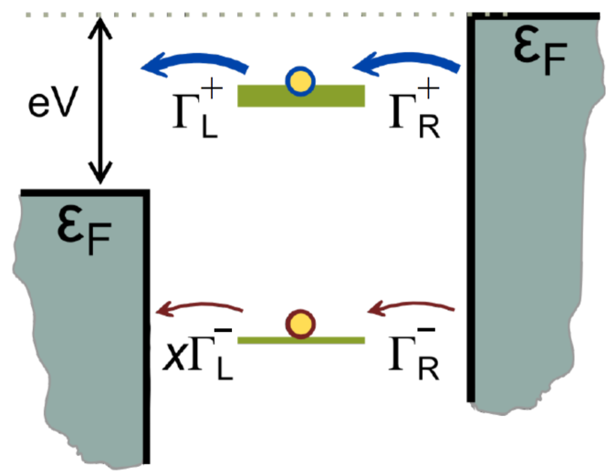
Figure 1: Schematic of the tunnel junction with two-level quantum dot considered in this paper.

The key property of the model belzig05 is an assumption that the low-energy level $\varepsilon_{-}$ of the dot is below the Fermi level of left electrode (and thus also of the right electrode), as shown schematically in Fig. 1. Hence, at $T=0$ there is no tunneling of electron to the left (and also to the right) from the dot, and the junction is completely blocked. At nonzero temperatures there are possible hopping processes to the left, which should be taken into account. This is accounted for by a temperature-dependent factor $x$ which describes tunneling to the left at the energy, at which all electron states in the left electrodes are filled at $T=0$ (Fig. 1), but may be empty at higher temperatures. We consider the case of $T\neq 0$ and assume that the density of temperature-activated holes in the left electrode is relatively small, so the parameter $x$ can be evaluated as $x\sim\exp[(\varepsilon_{-}-E_{F})/k_{B}T]\ll 1$.

To calculate the shot noise in junctions under consideration, we follow the method of FCS calculations proposed by Bagrets and Nazarov.bagrets03 First, we need to find the probability of quantum dot to be in one of the possible quantum states, which can be found from the following master equation describing dynamics of the dot’s states:

$$\frac{d{\bf P}}{dt}=\hat{M}{\bf P},$$ (1)

where

$${\bf P}^{T}=\left(P^{-}_{\uparrow},\,P^{-}_{\downarrow},\,P^{+}_{\uparrow},\,P^{+}_{\downarrow},\,P_{0}\right)$$ (2)

is a vector whose components describe probabilities of the dot to be in the state with one spin-$\sigma$ electron in the low-energy level ($P^{-}_{\sigma}$), one spin-$\sigma$ electron in the high-energy level ($P^{+}_{\sigma}$), and the probability of the state with no electrons in the dot ($P_{0}$).

As already mentioned above, the state with two excess electrons in the dot is assumed to have rather high energy due to strong electron correlations, so it is ruled out from the considerations. This assumption is well justified when QDs are sufficiently small. In our case we consider tunneling through short molecules which play a role of QDs. Coulomb energy of doubly charged molecules is then sufficiently large, so the above assumption is reasonable and well justified.

The matrix $\hat{M}$ on the right side of the master equation (1) includes the rates $\Gamma^{\pm}_{L\sigma}$ and $\Gamma^{\pm}_{R\sigma}$ of electron tunneling from the dot to the left electrode and from the right electrode to the dot, respectively,

$$\hat{M}=\left(\begin{array}[]{ccccc}-x\Gamma^{-}_{L\uparrow}&0&0&0&\Gamma^{-}_{R\uparrow}\\ 0&-x\Gamma^{-}_{L\downarrow}&0&0&\Gamma_{R\downarrow}^{-}\\ 0&0&-\Gamma^{+}_{L\uparrow}&0&\Gamma^{+}_{R\uparrow}\\ 0&0&0&-\Gamma^{+}_{L\downarrow}&\Gamma^{+}_{R\downarrow}\\ x\Gamma^{-}_{L\uparrow}&x\Gamma^{-}_{L\downarrow}&\Gamma^{+}_{L\uparrow}&\Gamma^{+}_{L\downarrow}&-\Gamma_{\Sigma}\end{array}\right),$$ (8)

where we also introduced the notation $\Gamma_{\Sigma}=\Gamma_{R\uparrow}^{+}+\Gamma_{R\uparrow}^{-}+\Gamma_{R\downarrow}^{+}+\Gamma_{R\downarrow}^{-}$. Since the electrodes are ferromagnetic, the tunneling probabilities are assumed to be dependent on the electron spin orientation. The signs ascribed to the elements of the matrix $\hat{M}$ correspond to increasing or decreasing probability of the corresponding dot state due to the respective tunneling processes. The factor $x$ in this matrix was already defined above and is assumed to be small, $x\ll 1$.

To distinguish between the probabilities of electron tunneling from the right electrode to the upper or to the lower energy level of the dot, we introduced different parameters $\Gamma_{R\sigma}^{+}$ and $\Gamma_{R\sigma}^{-}$. This difference can be attributed to different shapes of the electronic orbitals corresponding to the dot’s states. Transmission of electrons in the tunneling structure shown in Fig. 1 is a stochastic process, which consists of random hoppings of electrons between electrodes and QD at random times $\tau_{i}$. Therefore, the calculation of mean current, say through the left junction, as well as of current correlation functions imply averaging over processes $\zeta_{s}$ with an arbitrary number $s$ of sequential transitions with electron transfer in all possible channels. The probability $Q_{s}$ of the process $\zeta_{s}$ is determined by the probabilities of system to stay in certain states during the time between transitions and by the probability of single transitions at $\tau_{i}$ ($i=1,...s$) specified by the process $\zeta_{s}$. The probabilities of particular transitions are the matrix elements in Eq. (3). To find the generating function $S(\chi)$ of cumulant expansion one has to average the exponent $\exp\{i\int d\tau\,\chi(\tau)\,\hat{I}(\tau)\}$, where $\hat{I}(\tau)$ is an instanteneous current at $\tau$ and $\chi(\tau)$ is the source field introduced to find current cumulants by using the generating function $S(\chi)$. The key point of the theory in Ref. bagrets03, is that averaging of expression for the generating function with source field $\chi$ induces $\chi$-dependent probabilities $Q^{\chi}_{s}$ which differ from $Q_{s}$ by an exponential factor $e^{i\chi(\tau)}$ in the probability of tunneling through the considered (left) junction. All the details of this derivation can be found in the cited work.

Thus, following the method of Ref. bagrets03, , we consider eigenvalues of the matrix $\hat{Z}(\chi)$ defined as

$$\hat{Z}(\chi)=\left(\begin{array}[]{ccccc}-x\Gamma^{-}_{L\uparrow}&0&0&0&\Gamma_{R\uparrow}^{-}\\ 0&-x\Gamma^{-}_{L\downarrow}&0&0&\Gamma_{R\downarrow}^{-}\\ 0&0&-\Gamma^{+}_{L\uparrow}&0&\Gamma^{+}_{R\uparrow}\\ 0&0&0&-\Gamma^{+}_{L\downarrow}&\Gamma^{+}_{R\downarrow}\\ x\Gamma^{-}_{L\uparrow}e^{i\chi}&x\Gamma^{-}_{L\downarrow}e^{i\chi}&\Gamma^{+}_{L\uparrow}e^{i\chi}&\Gamma^{+}_{L\downarrow}e^{i\chi}&-\Gamma_{\Sigma}\end{array}\right).\hskip 11.38092pt$$ (14)

As compared to $\hat{M}$, the matrix $\hat{Z}(\chi)$ includes an additional phase factor $e^{i\chi}$, which allows to determine the generating function $S(\chi)$ of the current correlators,

$$S(\chi)=-t_{0}\lambda_{0}(\chi),$$ (15)

where $t_{0}$ is the period of transfer of a charge, and $\lambda_{0}(\chi)$ is the lowest eigenvalue of the matrix $\hat{Z}(\chi)$,

$$\det[\hat{Z}(\chi)-\lambda]=0.$$ (16)

In the case of $x=0$ (which corresponds to $T=0$) one obtains from Eq. (6) that the minimum eigenvalue of $\hat{Z}(\chi)$ is $\lambda_{0}=0$. Thus, for small $x$, $x\to 0$, one may look for a solution which is linear in $x$, $\lambda_{0}=x\tilde{\lambda}$. Using then Eqs. (4) and (6) we find the following algebraic equation for $\tilde{\lambda}$:

$$(\Gamma^{-}_{L\uparrow}+\tilde{\lambda})(\Gamma^{-}_{L\downarrow}+\tilde{\lambda})[(\Gamma^{+}_{R\uparrow}+\Gamma^{+}_{R\downarrow})(-1+e^{i\chi})-\Gamma_{R\uparrow}^{-}-\Gamma_{R\downarrow}^{-}]$$

$$+e^{i\chi}(\Gamma^{-}_{L\uparrow}+\tilde{\lambda})\Gamma^{-}_{L\downarrow}\Gamma^{-}_{R\downarrow}+e^{i\chi}(\Gamma^{-}_{L\downarrow}+\tilde{\lambda})\Gamma^{-}_{L\uparrow}\Gamma^{-}_{R\uparrow}=0.\hskip 8.5359pt$$ (17)

This is a quadratic equation for $\tilde{\lambda}$, which can be presented as $\tilde{\lambda}^{2}+2b\tilde{\lambda}+c=0$, where

$$b = \frac{(\Gamma^{-}_{L\uparrow}\Gamma^{-}_{R\uparrow}+\Gamma^{-}_{L\downarrow}\Gamma^{-}_{R\downarrow})\,e^{i\chi}}{2[(\Gamma^{+}_{R\uparrow}+\Gamma^{+}_{R\downarrow})(e^{i\chi}-1)-\Gamma^{-}_{R\uparrow}-\Gamma^{-}_{R\downarrow}]}$$ (18)

$$+\frac{\Gamma^{-}_{L\uparrow}+\Gamma^{-}_{L\downarrow}}{2}\,,$$

$$c = \Gamma^{-}_{L\uparrow}\Gamma^{-}_{L\downarrow}\,\frac{(e^{i\chi}-1)(\Gamma^{+}_{R\uparrow}+\Gamma^{+}_{R\downarrow}+\Gamma_{R\uparrow}^{-}+\Gamma_{R\downarrow}^{-})}{(\Gamma^{+}_{R\uparrow}+\Gamma^{+}_{R\downarrow})(e^{i\chi}-1)-\Gamma^{-}_{R\uparrow}-\Gamma^{-}_{R\downarrow}}\,.$$ (19)

Thus, the FCS generating function in the limit of low $T$ (small $x$) can be written as

$$S(\chi)=-t_{0}x\,\big{(}-b\pm\sqrt{b^{2}-c}\big{)},$$ (20)

with the parameters $b$ and $c$ defined by Eqs. (8) and (9).

III Electric current shot noise

The mean value of electric current, $\overline{I}$, and the correlator of current fluctuations (shot noise), $S_{2}$, are determined by the first two cumulants $C_{n}$ ($n=1,2$) of the generating function, $C_{n}=-(-i)^{n}[d^{n}S(\chi)/d\chi^{n}]|_{\chi=0}$, i.e. explicitly

$$\overline{I}=ieS^{\prime}(\chi)|_{\chi=0}$$ (21)

$$S_{2}=\overline{(I-\overline{I})^{2}}=2e^{2}S^{\prime\prime}(\chi)|_{\chi=0},$$ (22)

respectively, where $S^{\prime}(\chi)$ and $S^{\prime\prime}(\chi)$ stand for the first and second derivative of $S$ with respect to $\chi$. Obviously, the FCS method gives the possibility to calculate all higher current correlation functions, $S_{3}$, $S_{4}$, etc.

Using Eqs. (8)-(12) one finds the following expression for the mean value of electric current (we take the units with $t_{0}=1$):

$$\overline{I}=\frac{ex\Gamma^{-}_{L\uparrow}\Gamma^{-}_{L\downarrow}(\Gamma^{+}_{R\uparrow}+\Gamma^{+}_{R\downarrow}+\Gamma_{R\uparrow}^{-}+\Gamma_{R\downarrow}^{-})}{\Gamma^{-}_{L\uparrow}\Gamma_{R\downarrow}^{-}+\Gamma^{-}_{L\downarrow}\Gamma_{R\uparrow}^{-}}\,.\hskip 8.5359pt$$ (23)

We recall that the above expression is valid in the low temperature limit, where $x\ll 1$. Similarly, once can also determine the relevant shot noise $S_{2}$. Since the corresponding formula is relatively long, we present it in Appendix, see Eq.(A12), where we also give more details on its derivation. Having found the shot noise, one can determine the corresponding Fano factor,

$$F=\frac{C_{2}}{C_{1}}=\frac{S_{2}}{2e\overline{I}}=\frac{2(\Gamma^{+}_{R\uparrow}+\Gamma^{+}_{R\downarrow})+\Gamma_{R\uparrow}^{-}+\Gamma_{R\downarrow}^{-}}{(\Gamma_{R\uparrow}^{-}+\Gamma_{R\downarrow}^{-})}\hskip 14.22636pt$$

$$+\frac{2(\Gamma^{-}_{L\uparrow}\Gamma_{R\uparrow}^{-}+\Gamma^{-}_{L\downarrow}\Gamma_{R\downarrow}^{-})(\Gamma^{+}_{R\uparrow}+\Gamma^{+}_{R\downarrow}+\Gamma_{R\uparrow}^{-}+\Gamma_{R\downarrow}^{-})}{(\Gamma_{R\uparrow}^{-}+\Gamma_{R\downarrow}^{-})(\Gamma^{-}_{L\uparrow}\Gamma_{R\downarrow}^{-}+\Gamma^{-}_{L\downarrow}\Gamma_{R\uparrow}^{-})}$$

$$-\frac{2\Gamma^{-}_{L\uparrow}\Gamma^{-}_{L\downarrow}(\Gamma^{+}_{R\uparrow}+\Gamma^{+}_{R\downarrow}+\Gamma_{R\uparrow}^{-}+\Gamma_{R\downarrow}^{-})(\Gamma_{R\uparrow}^{-}+\Gamma_{R\downarrow}^{-})}{(\Gamma^{-}_{L\uparrow}\Gamma_{R\downarrow}^{-}+\Gamma^{-}_{L\downarrow}\Gamma_{R\uparrow}^{-})^{2}}\,.$$ (24)

In the nonmagnetic case, $\Gamma_{L\uparrow}^{\pm}=\Gamma_{L\downarrow}^{\pm}=\Gamma_{L}$ and $\Gamma_{R\uparrow}^{\pm}=\Gamma_{R\downarrow}^{\pm}=\Gamma_{R}$, we obtain the results of Ref. belzig05, , with the lowest two cumulants and the Fano factor equal

$$C_{1}=2x\Gamma_{L},\,C_{2}=6x\Gamma_{L},\,{\rm and}\,\;F=C_{2}/C_{1}=3.$$ (25)

Thus, the corresponding shot noise is then super-Poissonian, with $F=3$. If we take into account the spin dependence of electron tunneling, but assume $\Gamma_{R\sigma}^{-}=\Gamma_{R\sigma}^{+}$, then we find from Eq. (15) that the Fano factor is even larger than 3, $F>3$, for any choice of other parameters.

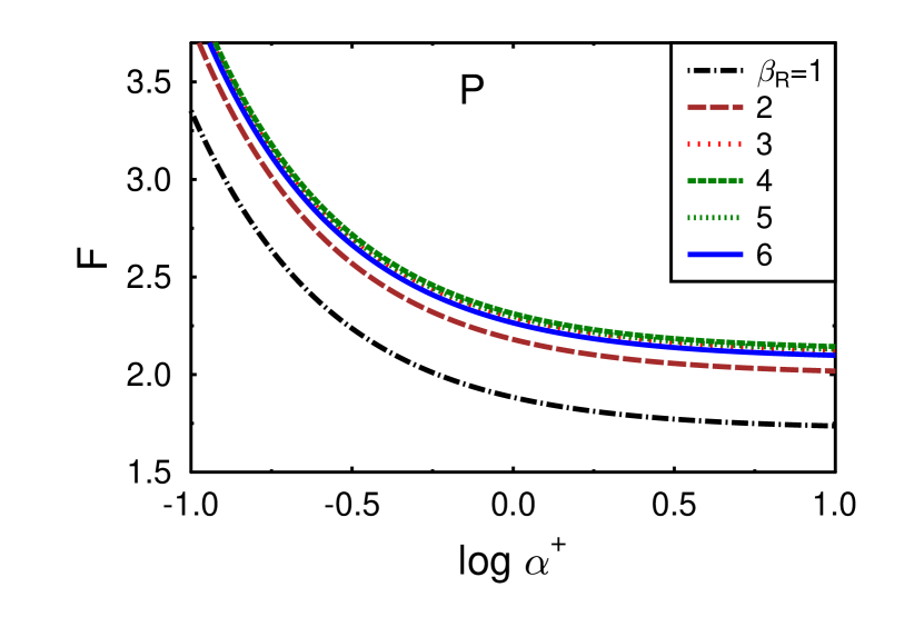
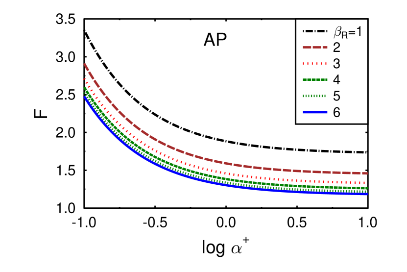
Figure 2: Fano factor in the parallel (top) and antiparallel (bottom) magnetic configurations as a function of $\alpha^{+}$. The other parameters are $x_{R}=0.3$, $x_{L}=1$, $\beta_{L}=4$, $\alpha^{-}=0.2$, and $\beta_{R}$ as indicated.

One can describe the shot noise and the Fano factor (15) by a certain number of parameters which quantify the relevant asymmetry in each of the transport channels. To do this let us define the junction resistance $R_{{L,R}\sigma}^{\pm}$ for each level- and spin-channel. The resistance $R_{{L,R}\sigma}^{\pm}$ is inversely proportional to the corresponding tunneling rate $\Gamma_{{L,R}\sigma}^{\pm}$. Accordingly, we introduce the parameters $\alpha^{+}=R_{R\uparrow}^{+}/R_{L\uparrow}^{+}$ and $\alpha^{-}=R_{R\uparrow}^{-}/R_{L\uparrow}^{-}$ to describe the right-left asymmetry, in the spin-up channel associated with the high-energy and low-energy dot’s levels. Apart from this, we also define the parameters $\beta_{R}=R_{R\downarrow}^{-}/R_{R\uparrow}^{-}$ and $\beta_{L}=R_{L\downarrow}^{-}/R_{L\uparrow}^{-}$ for the spin asymmetry in the coupling of the low-energy dot’s level to the leads. To describe a difference in the coupling of the two levels of the dot to the right electrode, we introduce the parameter $x_{R}$ defined as $x_{R}=R_{R\uparrow}^{-}/R_{R\uparrow}^{+}$. Similar parameter is also introduced to describe asymmetry of the coupling of the two levels to the left electrode, $x_{L}=R_{L\uparrow}^{-}/R_{L\uparrow}^{+}$.

In case of magnetic electrodes, we also distinguish between the parallel (P) and antiparallel (AP) arrangements of the magnetic moments of both electrodes. For definiteness, we define the spin-up orientation as the orientation of majority spins in the left electrode (i.e., opposite to magnetization vector in the left electrode), and assume that magnetic moment of the right electrode is reversed in the AP configuration. Thus, in the AP configuration the spin-up and spin-down electrons in the right electrode correspond to the spin-minority and spin-majority electrons, respectively.

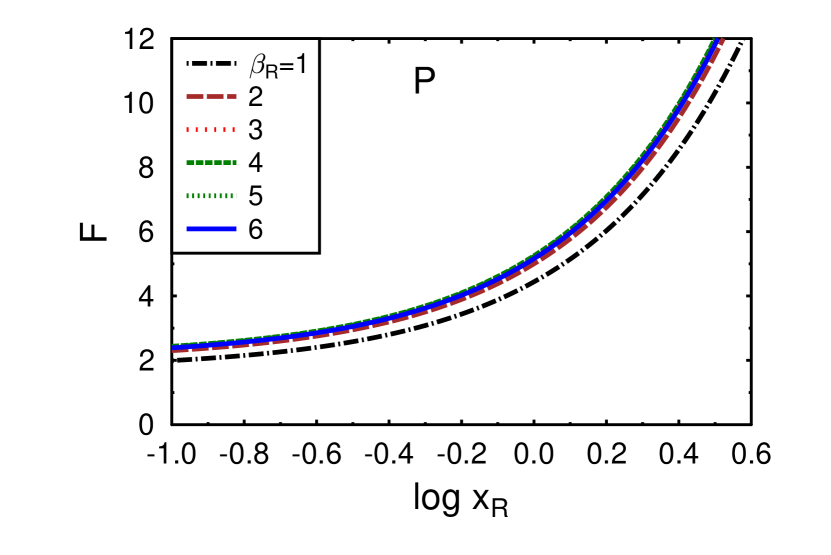
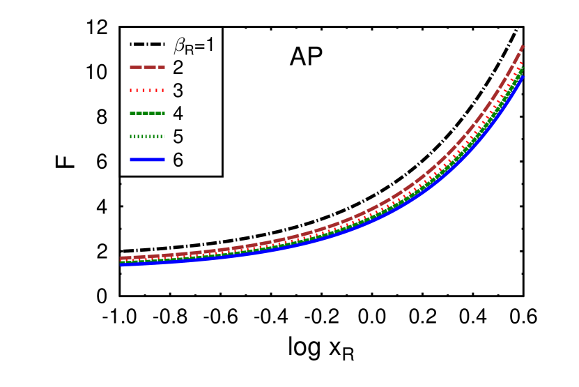
Figure 3: Fano factor in the parallel (top) and antiparallel (bottom) configurations as a function of $x_{R}$ for $\alpha^{+}=\alpha^{-}=1$, $x_{L}=1$, $\beta_{L}=4$, and $\beta_{R}$ as indicated.

Variation of the Fano factor $F$ with the parameter $\alpha^{+}=R_{R\uparrow}^{+}/R_{L\uparrow}^{+}$ in the P and AP configurations is shown in Fig. 2 for different values of the parameter $\beta_{R}$. Two features immediately follow from this figure. First, the shot noise and thus also the Fano factor are strongly enhanced when $\alpha^{+}<<1$, i.e. for $R_{R\uparrow}^{+}<<R_{L\uparrow}^{+}$. This is because a spin-up electron tunneling from the source (right) electrode to the high-energy level spends relatively long time before tunneling further to the sink (left) electrode, blocking this way electronic transport via other channels. Second, the Fano factor in the parallel configuration is generally larger than in the antiparallel state. Note, that for $\beta_{R}=1$ the parallel and antiparallel configurations are equivalent (right electrode is then nonmagnetic). Then, when $\beta_{R}>1$, the Fano factor in the parallel configuration is lower while in the antiparallel state is higher, which is in agreement with earlier observations.cascales14 In turn, dependence of the Fano factor on the parameters $x_{R}=R_{R\uparrow}^{-}/R_{R\uparrow}^{+}$ is shown in Fig. 3 for both magnetic configurations. The noise is super-Poissonian and the Fano factor is relatively large for $x_{R}>>1$, i.e. for $R_{R\uparrow}^{-}>>R_{R\uparrow}^{+}$. Again, the noise is smaller in the antiparallel configuration.

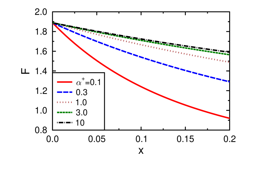
Figure 4: Dependence of the Fano factor on the temperature factor $x$ in the P configuration for $\alpha^{-}=0.3$ and different values of $\alpha^{+}$. The other parameters are $x_{R}=0.3$, $x_{L}=1$, $\beta_{R}=2$, and $\beta_{L}=4$.

When the temperature increases, the parameter $x$ in Eq. (3) also increases, which leads to the temperature dependence of the Fano factor. The simple algebraic method presented above can not be used now. Hence, we calculated numerically the eigenvalues of the matrix $\hat{Z}(\chi)$, Eq. (4), and used the lowest eigenvalue $\lambda_{0}$ of the matrix $\hat{Z}(\chi)$ to determine the first two cumulants and thus the Fano factor, $F=C_{2}/C_{1}$. The dependence of $F$ on the temperature-dependent parameter $x$ is presented in Fig. 4. The low-temperature limit of the Fano factor $F$ corresponds to $x\to 0$. The magnitude of Fano factor essentially decreases with increasing temperature. This is related to de-blocking of the conduction channel through the low-energy level $E_{-}$. Note, the system may go to the sub-Poissonian regime with increasing temperature.

IV Spin current noise

The FCS method for calculation of current and current noise can be easily generalized to study the spin current and spin current noise. To do this we consider the eigenvalues of the matrix $\hat{Z}_{s}(\chi)$, which we define as

$$\hat{Z}_{s}(\chi)=\left(\begin{array}[]{ccccc}-x\Gamma^{-}_{L\uparrow}&0&0&0&\Gamma_{R\uparrow}^{-}\\ 0&-x\Gamma^{-}_{L\downarrow}&0&0&\Gamma_{R\downarrow}^{-}\\ 0&0&-\Gamma^{+}_{L\uparrow}&0&\Gamma^{+}_{R\uparrow}\\ 0&0&0&-\Gamma^{+}_{L\downarrow}&\Gamma^{+}_{R\downarrow}\\ x\Gamma^{-}_{L\uparrow}e^{i\chi}&x\Gamma^{-}_{L\downarrow}e^{-i\chi}&\Gamma^{+}_{L\uparrow}e^{i\chi}&\Gamma^{+}_{L\downarrow}e^{-i\chi}&-\Gamma_{\Sigma}\end{array}\right).\hskip 5.69046pt$$ (31)

In contrast to Eq. (4), we count here the hopping through the left junction of spin-up and spin-down electrons, corresponding to the plus and minus sings in the exponents in the bottom row, respectively. This means that we calculate the spin current as a difference of the fluxes of electrons in the spin-up and spin-down channels.

Figure 5: Spin polarization of current $I_{s}/I$ as a function for $\beta_{R}$ in P (top) and AP (bottom) configurations. The other parameters are $x_{R}=0.3$, $x_{L}=1$, $\alpha^{+}=0.3$, $\alpha^{-}=0.2$, and $\beta_{L}=4$.

All the calculations are similar to those in the case of electric current, so we will not repeat the details, but present only some results. In the low-temperature limit ($x\to 0$) the first two cumulants can be written in the form

$$C_{1}^{s}\simeq\frac{x\Gamma^{-}_{L\uparrow}\Gamma^{-}_{L\downarrow}(\Gamma^{+}_{R\uparrow}+\Gamma^{-}_{R\uparrow}-\Gamma^{+}_{R\downarrow}-\Gamma^{-}_{R\downarrow})}{\Gamma^{-}_{L\uparrow}\Gamma^{-}_{R\downarrow}+\Gamma^{-}_{L\downarrow}\Gamma^{-}_{R\uparrow}}\,,\hskip 14.22636pt$$ (32)

$$C_{2}^{s}\simeq\frac{2x\Gamma^{-}_{L\uparrow}\Gamma^{-}_{L\downarrow}}{\Gamma^{-}_{L\uparrow}\Gamma^{-}_{R\downarrow}+\Gamma^{-}_{L\downarrow}\Gamma^{-}_{R\uparrow}}\left\{\frac{1}{2}(\Gamma^{+}_{R\downarrow}+\Gamma^{-}_{R\downarrow}+\Gamma^{+}_{R\uparrow}+\Gamma^{-}_{R\uparrow})\right.$$

$$\left.+(\Gamma^{+}_{R\downarrow}+\Gamma^{-}_{R\downarrow}-\Gamma^{+}_{R\uparrow}-\Gamma^{-}_{R\uparrow})\frac{\Gamma^{+}_{R\downarrow}-\Gamma^{+}_{R\uparrow}}{\Gamma^{-}_{R\uparrow}+\Gamma^{-}_{R\downarrow}}\right.$$

$$\left.+\left[\Gamma^{-}_{L\downarrow}\Gamma^{-}_{R\downarrow}-\Gamma^{-}_{L\uparrow}\Gamma^{-}_{R\uparrow}+(\Gamma^{-}_{L\downarrow}\Gamma^{-}_{R\downarrow}+\Gamma^{-}_{L\uparrow}\Gamma^{-}_{R\uparrow})\frac{\Gamma^{+}_{R\downarrow}-\Gamma^{+}_{R\uparrow}}{\Gamma^{-}_{R\uparrow}+\Gamma^{-}_{R\downarrow}}\right]\right.$$

$$\left.\times\frac{\Gamma^{+}_{R\downarrow}+\Gamma^{-}_{R\downarrow}-\Gamma^{+}_{R\uparrow}-\Gamma^{-}_{R\uparrow}}{\Gamma^{-}_{L\uparrow}\Gamma^{-}_{R\downarrow}+\Gamma^{-}_{L\downarrow}\Gamma^{-}_{R\uparrow}}-\Gamma^{-}_{L\uparrow}\Gamma^{-}_{L\downarrow}(\Gamma^{-}_{R\uparrow}+\Gamma^{-}_{R\downarrow})\right.$$

$$\left.\times\left(\frac{\Gamma^{+}_{R\downarrow}+\Gamma^{-}_{R\downarrow}-\Gamma^{+}_{R\uparrow}-\Gamma^{-}_{R\uparrow}}{\Gamma^{-}_{L\uparrow}\Gamma^{-}_{R\downarrow}+\Gamma^{-}_{L\downarrow}\Gamma^{-}_{R\uparrow}}\right)^{2}\right\}.\hskip 11.38092pt$$ (33)

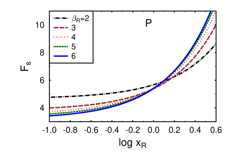
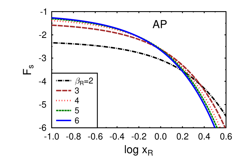
Figure 6: Spin Fano factor in the parallel (top) and antiparallel (bottom) configurations as a function of $x_{R}$ for $\alpha^{+}=\alpha^{-}=1$, $x_{L}=1$, $\beta_{L}=4$, and $\beta_{R}$ as indicated.

Accordingly, the mean spin current can be calculated as $I_{s}=C_{1}^{s}$, while the spin current noise as $S_{2}^{s}=2C_{2}^{s}$. In Fig. 5 we present the spin polarization of electric current $I_{s}/I=C_{1}^{s}/C_{1}$ in the P and AP configurations. As we see, the polarization strongly depends on the parameter $\beta_{R}$ describing asymmetry between the spin-up and spin-down channels.

In Fig. 6 we show the calculated spin Fano factor, defined as $F_{s}=C_{2}^{s}/C_{1}^{s}$, for both parallel and antiparallel magnetic configurations. These Fano factors are presented as a function of $x_{R}$. In the parallel configuration the Fano factor increases with increasing $x_{R}$ while in the antiparallel state it decreases with increasing $x_{R}$. Note, the spin Fano factor is positive in the P configuration and negative in the AP state. This difference is associated with different signs of the spin current in the two configurations.

V Experimental data on shot noise in magnetic tunnel junctions

Experimental measurements of shot noise have been performed in magnetic tunnel junctions with molecular perylene-teracarboxylic dianhydride (PTCDA) organic barriers. The molecular layer was up to 5 nm thick. The shot noise measurements have been done at 0.3 K and for the bias up to 10 mV. Detailed description of the preparation method of the tunnel junctions and of the experimental technique used to measure shot noise have been published elsewhere. li11

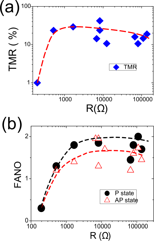
Figure 7: (a) Tunneling magnetoresistance of OMTJs with PTCDA barriers with different PTCDA thickness ranging from 0 nm (1.2 nm of AlO_x buffer layers only) to 5 nm and plotted as a function of device resistance (low bias junction resistance in the P state). Measurements have been done at 10 K and with applied bias of 1 mV (b) Fano factor in the P and AP states as a function of OMTJs resistance measured at T=0.3 K and averaged for the bias range about 3-10 mV. Dashed lines are guides for the eye.

Representative experimental results are shown in Fig. 7. More experimental data can be found in Ref. cascales14, . We have measured not only the shot noise and the corresponding Fano factor, but also the tunneling magnetoresistance (TMR). The latter is defined as the relative difference in the junction resistances in antiparallel and parallel magnetic configurations. As one can see in Fig. 7a, the organic magnetic tunnel junctions (OMTJs) show TMR ratio ranging between 10% and 40%, with the lowest value of TMR observed in the PTCDA-free samples, i.e. in the sample with no PTCDA layer, but with 1.2 nm AlO_x tunnel barrier only. The experimental values of TMR are in agreement with the model calculations for the parameter $\beta_{R}\simeq 1.6$.cascales14 Note, the TMR ratio in Fig. 7 is shown as a function of low bias junction resistance in the P state. Previous measurements indicated approximately exponential dependence of the junction resistance on the PTCDA thickness. cascales14

The measurements of shot noise reveal super-Poissonian tunneling statistics, with the Fano factor ranging between 1.5 and 2 when the barrier includes the PTDCA layer (see also the preliminary reportcascales14 ). The control sample (i.e., the sample without PTCDA but with 1.2 nm AlO_x tunnel barrier only) shows the lowest resistance and also the lowest Fano factor of the order of $F$=0.3 (which corresponds to the sub-Poissonian statistics), as expected for disordered metals. Hence, we conclude that the super-Poissonian shot noise observed in OMTJs is most likely associated with tunneling through discrete states. The measured Fano factors in both magnetic configurations are shown in Fig. 7b for 3-10 mV biased junctions. The data are also presented as a function of the junction resistance. As already reported earlier, the Fano factors in the AP state are smaller than in the P one.

In order to account for the experimental observation of the shot noise in OMTJs, we have proposed cascales14 a theoretical model based on tunneling through a two-level systems, like that presented above. Taking into account the fact that the super-Poissonian shot noise appears mainly at larger voltages, such a two-level system may be attributed to interfacial states of the PTCDA molecules in a biased junction. Indeed, the experimental results can be quite well explained qualitatively and also quantitatively in terms of the model based on spin-dependent electron tunneling through an interacting two-level system, described in detail in the preceding sections. In order to qualitatively account for the experimentally observed situation with the Fano factor in the AP state (on the average, we observe $F=1.5$) being smaller than the Fano factor in the P state (1.7), we did numerical calculations based on the model presented above, see Fig. 2, and from fitting to the experimental data we evaluated the parameters that reproduce the Fano factors in both configurations.

VI Discussions

The results of our calculations are in qualitative agreement with the physical interpretation given in Ref. belzig05, . Indeed, considering the simplest two-level model (Fig. 1) it was concluded that the generating function $S(\chi)$ can be presented as a sum of independent Poissonian processes of transferring $ne$ charges with probability of $(1/2)^{n}$ with $n=1$ to $\infty$. In turn, the process of transferring $ne$ charges with large $n$ during one cycle is possible because the tunneling to the left lead from the lower level is strongly suppressed by the temperature factor $(1-f(\varepsilon_{-}))$. In other words, several electrons can be quickly transferred through the upper level till the cycle is stopped by an electron at the lower level. This is a super-Poissonian process, and the Fano factor is equal to 3.

In our calculations we used the model of QDs with two energy levels, when one of them is located below the Fermi level of left electrode $\varepsilon_{FL}$, and the other one is between the Fermi levels of left and right electrodes. In reality the QD or molecule can have many energy levels, with part of them situated below $\varepsilon_{FL}$ and another part between $\varepsilon_{FL}$ and $\varepsilon_{FR}$. It is rather obvious that this is not so important for the mechanism of super-Poissonian noise related to blocking of electron transport through the low energy level. Generalization to the multilevel system with $N_{+}$ upper and $N_{-}$ lower levels (bunched in two blocks with the same tunneling probability in each block) can change the statistics, so that $F=(1+p)/(1-p)$, where $p=N_{+}/(N_{+}+N_{-})$. In particular, for $p=1/2$ we obtain again $F=3$. In this multilevel model, one can also get $F=2$ with $p=1/3$, which corresponds to $N_{-}=2N_{+}$ (e.g., lower level is twice degenerate and the upper one is nondegenerate). In the case of nonmagnetic system, each of the levels is spin degenerate. Thus, assuming equal tunneling probabilities for the spin-up and spin-down electrons, one would get $p=1/2$ and $F=3$.

We also assumed that the tunneling probabilities are different for the lower and upper levels. This changes essentially the result for the Fano factor because the probability of transferring $ne$ electrons includes now the weight factor of the ratio $(\Gamma^{-}_{R}/\Gamma_{R})^{n}$ since the probability of tunneling of a single electron from the right lead to the upper level is not equal to $1/2$ anymore. In other words, the transfer of electrons through the upper level can be not so quick due to a lower probability of the corresponding tunneling, and this partially suppresses the super-Poissonian process as a sum of Poissonian processes with the transfer of multiple charges.

Within this approach one can also consider electron tunneling through a chain of molecules in relatively thick junctions. Now the energy levels of different molecules are not exactly at the same energy. First, because there is a potential slope within the junction, which shifts correspondingly all the energy levels in the junction. Second, due to inevitable disorder, there exist some fluctuations of potential. This means that the intermolecular tunneling can be possible only due to emission or absorption of appropriate phonons. In this situation one can expect that there is only one ’optimal’ path of the electron transfer through the chain of molecules, which uses a chosen number of the energy levels. The probability of charge transfer through other pathes is exponentially small since it requires substantial energy change at each intermolecular tunneling. Hence, we come back to a Poissonian process of the transfer of a single charge through the molecular chain. In this case we naturally obtain $F=1$.

It is also worth noting, that the super-Poissonian noise can appear due to other physical mechanisms as well, for example due to electron-phonon or electron-electron interactions.blanter00 However, the mechanism proposed by Belzig belzig05 and based on tunneling through two or more discrete levels is the most appropriate one in our case. Indeed, the assumption of tunneling through discrete levels (with one low-energy level) is physically reasonable and justified. Moreover, this model explains the possibility of a rather strong enhancement of the Fano factor, and is also able to account for the experimental observations in the studied system.

Appendix A Calculation of the shot noise

Using the expression for $\tilde{\lambda}(\chi)$

$$\tilde{\lambda}(\chi)=-b\pm\sqrt{b^{2}-c}$$ (34)

we find

$$\tilde{\lambda}^{\prime}=-b^{\prime}\pm\frac{2bb^{\prime}-c^{\prime}}{2\sqrt{b^{2}-c}}\,,$$ (35)

$$\tilde{\lambda}^{\prime\prime}=-b^{\prime\prime}\pm\frac{2(b^{\prime})^{2}+2bb^{\prime\prime}-c^{\prime\prime}}{2\sqrt{b^{2}-c}}\mp\frac{(2bb^{\prime}-c^{\prime})^{2}}{4(b^{2}-c)^{3/2}}\,.\hskip 8.5359pt$$ (36)

In the limit of $\chi\to 0$ we get

$$b\simeq\frac{\Gamma_{L\uparrow}\Gamma_{R\downarrow}^{-}+\Gamma_{L\downarrow}\Gamma_{R\uparrow}^{-}}{2(\Gamma_{R\uparrow}^{-}+\Gamma_{R\downarrow}^{-})},$$ (37)

$$c\simeq 0,$$ (38)

$$b^{\prime}\simeq-\frac{i(\Gamma_{L\uparrow}\Gamma_{R\uparrow}^{-}+\Gamma_{L\downarrow}\Gamma_{R\downarrow}^{-})}{2(\Gamma_{R\uparrow}^{-}+\Gamma_{R\downarrow}^{-})^{2}}$$

$$\hskip 14.22636pt\times(\Gamma_{R\uparrow}+\Gamma_{R\downarrow}+\Gamma_{R\uparrow}^{-}+\Gamma_{R\downarrow}^{-}),$$ (39)

$$b^{\prime\prime}=\frac{(\Gamma_{L\uparrow}^{-}\Gamma_{R\uparrow}^{-}+\Gamma_{L\downarrow}^{-}\Gamma_{R\downarrow}^{-})(\Gamma_{R\uparrow}^{-}+\Gamma_{R\downarrow}^{-}+\Gamma_{R\uparrow}^{+}+\Gamma_{R\downarrow}^{+})}{(\Gamma_{R\uparrow}^{-}+\Gamma_{R\downarrow}^{-})^{2}}$$

$$\hskip 14.22636pt\times\left(\frac{1}{2}+\frac{\Gamma_{R\uparrow}^{+}+\Gamma_{R\downarrow}^{+}}{\Gamma_{R\uparrow}^{-}+\Gamma_{R\downarrow}^{-}}\right),$$ (40)

$$c^{\prime}\simeq-\frac{i\Gamma_{L\uparrow}\Gamma_{L\downarrow}(\Gamma_{R\uparrow}+\Gamma_{R\downarrow}+\Gamma_{R\uparrow}^{-}+\Gamma_{R\downarrow}^{-})}{\Gamma_{R\uparrow}^{-}+\Gamma_{R\downarrow}^{-}},$$ (41)

$$c^{\prime\prime}\simeq\frac{\Gamma_{L\uparrow}\Gamma_{L\downarrow}(\Gamma_{R\uparrow}+\Gamma_{R\downarrow}+\Gamma_{R\uparrow}^{-}+\Gamma_{R\downarrow}^{-})}{(\Gamma_{R\uparrow}^{-}+\Gamma_{R\downarrow}^{-})^{2}}$$

$$\hskip 28.45274pt\times[2(\Gamma_{R\uparrow}+\Gamma_{R\downarrow})+\Gamma_{R\uparrow}^{-}+\Gamma_{R\downarrow}^{-}].$$ (42)

Then we obtain the cumulants

$$C_{1}=iS^{\prime}(\chi)_{\chi=0}=\frac{x\Gamma_{L\uparrow}\Gamma_{L\downarrow}(\Gamma_{R\uparrow}+\Gamma_{R\downarrow}+\Gamma_{R\uparrow}^{-}+\Gamma_{R\downarrow}^{-})}{\Gamma_{L\uparrow}\Gamma_{R\downarrow}^{-}+\Gamma_{L\downarrow}\Gamma_{R\uparrow}^{-}}\,,\hskip 17.07182pt$$ (43)

$$C_{2}=S^{\prime\prime}(\chi)_{\chi=0}=x\Gamma_{L\uparrow}\Gamma_{L\downarrow}(\Gamma_{R\uparrow}+\Gamma_{R\uparrow}+\Gamma_{R\uparrow}^{-}+\Gamma_{R\downarrow}^{-})$$

$$\times\left[\frac{2(\Gamma_{R\uparrow}+\Gamma_{R\downarrow})+\Gamma_{R\uparrow}^{-}+\Gamma_{R\downarrow}^{-}}{(\Gamma_{R\uparrow}^{-}+\Gamma_{R\downarrow}^{-})(\Gamma_{L\uparrow}\Gamma_{R\downarrow}^{-}+\Gamma_{L\downarrow}\Gamma_{R\uparrow}^{-})}\right.$$

$$\left.+\frac{2(\Gamma_{L\uparrow}\Gamma_{R\uparrow}^{-}+\Gamma_{L\downarrow}\Gamma_{R\downarrow}^{-})(\Gamma_{R\uparrow}+\Gamma_{R\uparrow}+\Gamma_{R\uparrow}^{-}+\Gamma_{R\downarrow}^{-})}{(\Gamma_{R\uparrow}^{-}+\Gamma_{R\downarrow}^{-})(\Gamma_{L\uparrow}\Gamma_{R\downarrow}^{-}+\Gamma_{L\downarrow}\Gamma_{R\uparrow}^{-})^{2}}\right.$$

$$\left.-\frac{2\Gamma_{L\uparrow}\Gamma_{L\downarrow}(\Gamma_{R\uparrow}+\Gamma_{R\uparrow}+\Gamma_{R\uparrow}^{-}+\Gamma_{R\downarrow}^{-})(\Gamma_{R\uparrow}^{-}+\Gamma_{R\downarrow}^{-})}{(\Gamma_{L\uparrow}\Gamma_{R\downarrow}^{-}+\Gamma_{L\downarrow}\Gamma_{R\uparrow}^{-})^{3}}\right]\hskip 14.22636pt$$ (44)

and the explicit formula for shot noise $S_{2}$

$$S_{2}=2e^{2}x\Gamma^{-}_{L\uparrow}\Gamma^{-}_{L\downarrow}\big{(}\Gamma^{+}_{R\uparrow}+\Gamma^{+}_{R\downarrow}+\Gamma_{R\uparrow}^{-}+\Gamma_{R\downarrow}^{-}\big{)}\hskip 42.67912pt$$

$$\times\left[\frac{2(\Gamma^{+}_{R\uparrow}+\Gamma^{+}_{R\downarrow})+\Gamma_{R\uparrow}^{-}+\Gamma_{R\downarrow}^{-}}{(\Gamma_{R\uparrow}^{-}+\Gamma_{R\downarrow}^{-})(\Gamma_{L\uparrow}^{-}\Gamma_{R\downarrow}^{-}+\Gamma_{L\downarrow}^{-}\Gamma_{R\uparrow}^{-})}\right.$$

$$\left.+\frac{2(\Gamma^{-}_{L\uparrow}\Gamma_{R\uparrow}^{-}+\Gamma^{-}_{L\downarrow}\Gamma_{R\downarrow}^{-})(\Gamma^{+}_{R\uparrow}+\Gamma^{+}_{R\downarrow}+\Gamma_{R\uparrow}^{-}+\Gamma_{R\downarrow}^{-})}{(\Gamma_{R\uparrow}^{-}+\Gamma_{R\downarrow}^{-})(\Gamma^{-}_{L\uparrow}\Gamma_{R\downarrow}^{-}+\Gamma^{-}_{L\downarrow}\Gamma_{R\uparrow}^{-})^{2}}\right.$$

$$\left.-\frac{2\Gamma^{-}_{L\uparrow}\Gamma^{-}_{L\downarrow}(\Gamma^{+}_{R\uparrow}+\Gamma^{+}_{R\downarrow}+\Gamma_{R\uparrow}^{-}+\Gamma_{R\downarrow}^{-})(\Gamma_{R\uparrow}^{-}+\Gamma_{R\downarrow}^{-})}{(\Gamma^{-}_{L\uparrow}\Gamma_{R\downarrow}^{-}+\Gamma^{-}_{L\downarrow}\Gamma_{R\uparrow}^{-})^{3}}\right].\hskip 17.07182pt$$ (45)

References

- (1) S. Kogan, Electronic Noise and Fluctuations in Solids (Cambridge Univ. Press, Cambridge, 1996).
- (2) Ya. M. Blanter and M. Büttiker, Shot noise in mesoscopic conductors, Phys. Reports 336, 1 (2000).
- (3) Quantum Noise in Mesoscopic Physics, edited by Yu. V. Nazarov (Kliwer, Dordrecht, 2003).
- (4) L. D. Landau and E. M. Lifshitz, Statistical Physics (Pergamon Press, Oxford, 1980), Chap. 1.
- (5) W. Schottky, Über spontane Stromschwankungen in verschiedenen Elektrizitätsleitern, Ann. Phys. (Leipzig) 57, 541 (1918).
- (6) V. K. Khlus, Current and voltage fluctuations in microjunctions of normal and superconducting metals, Sov. Phys. JETP 66, 1243 (1987) [Zh. Eksp. Teor. Phys. 93, 2179 (1987)].
- (7) G. B. Lesovik, Excess quantum noise in 2D ballistic point contacts, JETP Lett. 49, 592 (1989).
- (8) M. Büttiker, Scattering theory of thermal and excess noise in open conductors, Phys. Rev. Lett. 65, 2901 (1990).
- (9) C. W. J. Beenakker and M. Büttiker, Suppression of shot noise in metallic diffusive conductors, Phys. Rev. B46, 1889 (1992).
- (10) L. S. Levitov and G. B. Lesovik, Charge-transport statistics in quantum conductors, Pis’ma v Zh. Eksp. Teor. Fiz. 55, 534 (1992) [JETP Lett. 55, 555 (1992)].
- (11) L. S. Levitov and G. B. Lesovik, Charge distribution in quantum shot noise, JETP Lett. 58, 230 (1993) [Pis’ma v Zh. Eksp. Teor. Fiz. 58, 225 (1993)].
- (12) D. A. Ivanov and L. S. Levitov, Statistics of charge fluctuations in quantum transport in an alternating field, Pis’ma v Zh. Eksp. Teor. Fiz. 58, 450 (1993) [JETP Lett. 58, 461 (1993)].
- (13) L. S. Levitov, H. Lee, and G. B. Lesovik, Electron counting statistics and coherent states of electric current, J. Math. Phys. 37, 4845 (1996).
- (14) D. A. Bagrets and Yu. V. Nazarov, Full counting statistics of charge transfer in Coulomb blockade regime, Phys. Rev. B67, 085316 (2003).
- (15) L. S. Levitov and M. Reznikov, Counting statistics of tunneling current, Phys. Rev. B70, 115305 (2004).
- (16) W. Belzig, Full counting statistics of super-Poissonian shot noise in multilevel quantum dots, Phys. Rev. B71, 161301(R) (2005).
- (17) K. Kaasbjerg and W. Belzig, Full counting statistics and shot noise of cotunneling in quantum dots and single-molecule transistors, Phys. Rev. B91, 235413 (2015).
- (18) W. Lu, Z. Ji, L. Pfeiffer, K. W. West, and A. J. Rimberg, Real-time detection of electron tunnelling in a quantum dot, Nature 423, 422 (2003).
- (19) T. Fujisawa, T. Hayashi, R. Tomita, and Y. Hirayama, Bidirectional counting of single electrons, Science 312, 1634 (2006).
- (20) C. Flindt, C. Fricke, F. Hohls, T. Novotný, K. Netocnýd, T. Brandese, and R. J. Haug, Universal oscillations in counting statistics, PNAS 106, 10116 (2009).
- (21) J. P. Cascales, J. Y. Hong, I. Martinez, M. T. Lin, T. Szczepański, V. K. Dugaev, J. Barnaś, and F. G. Aliev, Superpoissonian shot noise in organic magnetic tunnel junctions, Appl. Phys. Lett. 105, 233302 (2014).
- (22) E. G. Mishchenko, Shot noise in a diffusive ferromagnetic-paramagnetic-ferromagnetic spin valve, Phys. Rev. B68, 100409(R) (2003).
- (23) W. Belzig and M. Zareyan, Spin-flip noise in a multiterminal spin valve, Phys. Rev. B69, 140407(R) (2004).
- (24) A. Lamacraft, Shot noise of spin-polarized electrons, Phys. Rev. B, 69, 081301(R) (2004).
- (25) B. Wang, J. Wang, and H. Guo, Shot noise of spin current, Phys. Rev. B69, 153301 (2004).
- (26) O. Sauret and D. Feinberg, Spin-current shot noise as a probe of interactions in mesoscopic systems, Phys. Rev. Lett. 92, 106601 (2004).
- (27) J. Foros, A. Brataas, Y. Tserkovnyak, and G. E. W. Bauer, Magnetization noise in magnetoelectronic nanostructures, Phys. Rev. Lett. 95, 016601 (2005).
- (28) R. Guerrero, F. G. Aliev, Y. Tserkovnyak, T. S. Santos, and J. S. Moodera, Shot noise in magnetic tunnel junctions: Evidence for sequential tunneling, Phys. Rev. Lett. 97, 266602 (2006).
- (29) R. L. Dragomirova and B. K. Nikolić, Shot noise of spin-polarized charge currents as a probe of spin coherence in spin-orbit coupled nanostructures, Phys. Rev. B75, 085328 (2007).
- (30) A. L. Chudnovskiy, J. Swiebodzinski, and A. Kamenev, Spin-torque shot noise in magnetic tunnel junctions, Phys. Rev. Lett. 101, 066601 (2008).
- (31) J. P. Cascales, D. Herranz, F. G. Aliev, T. Szczepański, V.K. Dugaev, J. Barnaś, A. Duluard, M. Hehn, and C. Tiusan, Controlling shot noise in double-barrier magnetic tunnel junctions, Phys. Rev. Lett. 109, 066601 (2012).
- (32) T. Szczepański, V.K. Dugaev, J. Barnaś, J. P. Cascales, and F. G. Aliev, Shot noise in magnetic double-barrier tunnel junctions, Phys. Rev. B87, 155406 (2013).
- (33) G.-M. Tang and J. Wang, Full-counting statistics of charge and spin transport in the transient regime: A nonequilibrium Green’s function approach, Phys. Rev. B90, 195422 (2014).
- (34) H.-B. Xue, J.-Q. Liang, and W. M. Liu, Negative differential conductance and super-Poissonian shot noise in single-molecule magnet junctions, Scientific Rep. 5, 8730 (2015).
- (35) A. Burtzlaff, A. Weismann, M. Brandbyge, and R. Berndt, Shot noise as a probe of spin-polarised transport through single atoms, Phys. Rev. Lett. 114, 016602 (2015).
- (36) T. Arakawa, J. Shiogai, M. Ciorga, M. Utz, D. Schuh, M. Kohda, J. Nitta, D. Bougeard, D. Weiss, T. Ono, and K. Kobayashi, Shot noise induced by nonequilibrium spin accumulation, Phys. Rev. Lett. 114, 016601 (2015).
- (37) We call it quantum dot but it can be also a molecule if we do not account for possible phonon modes coupled to electrons states in molecules.
- (38) K. S. Li, Y. M. Chang, S. Agilan, J. Y. Hong, J. C. Tai, W. C. Chiang, K. Fukutani, P. A. Dowben, and M.-T. Lin, Organic spin valves with inelastic tunneling characteristics, Phys. Rev. B83, 172404 (2011).