Abstract

Deriving the optimal safety stock quantity with which to meet customer satisfaction is one of the most important topics in stock management. However, it is difficult to control the stock management of correlated marketable merchandise when using an inventory control method that was developed under the assumption that the demands are not correlated. For this, we propose a deterministic approach that uses a probability inequality to derive a reasonable safety stock for the case in which we know the correlation between various commodities. Moreover, over a given lead time, the relation between the appropriate safety stock and the allowable stockout rate is analytically derived, and the potential of our proposed procedure is validated by numerical experiments.

1 Introduction

Safety stock management is one of the most important issues related to inventory control. A well-known method is commonly used to determine the appropriate inventory, but it is based on the assumption that the demands for stock items are independent; thus, it is not appropriate when the demands are correlated. Moreover, it cannot be applied when the statistical properties (mean and variance,) of the demand distribution are unknown.

In recent years, various studies [1, 2, 3, 4] have actively investigated a novel approach to resolving this difficulty; it is based on a probability inequality, in particular, the Markov inequality or Chebyshev inequality, and derives the relation between the quantity of safety stock and the allowable stockout rate. For instance, Fotopoulos et al. discuss the relation between the safety stock quantity and the allowable stockout rate; they use the Chebyshev inequality, since the actual stockout rate becomes smaller than the average of the polynomial of demand [1]. Takemoto et al. [2] and Takemoto and Arizono [3] have used the Hoeffding inequality for the limited demand information, of which only the minimum and maximum values are known, and calculated the safety stock quantity which can guarantee a given allowable stockout rate. In particular, Takemoto and Arizono [3] assessed the stockout rate for the supply of two types of electric power, which were represented by two uncorrelated random variables. Shinzato and Kaku [4] derived an expression for the relation between the safety stock quantity and the allowable stockout rate. They considered the case in which the time series correlation (trend) in the demand sequence of one of the commodities was known; this information was included by using the Chernoff inequality. Although various studies have used a probability inequality to estimate the appropriate safety stock quantity, most analyses of safety stock have been for individual commodities or uncorrelated demands. However, in practice, stock management usually must address multiple commodities with correlated demands; this has not been sufficiently studied. In order to address this, we use the Chernoff inequality to derive the relation between the safety stock quantity and the allowable stockout rate, and we perform experiments that validate the effectiveness of our proposed method.

This paper is organized as follows. In section 2, we introduce the Chernoff inequality as a way to analytically estimate the stockout rate over the lead time. We then use this method to derive the relation between the safety stock quantity and the allowable stockout rate. In section 3, we use the statistical properties of the known demand distributions of two correlated commodities and conduct numerical simulations to verify the validity of our proposed approach. In section 4, we summarize our conclusions and discuss areas of future work on this topic.

2 Safety stock management and model setting

In this section, we begin by discussing an existing safety stock management policy that is based on the assumption that the distributions of the commodities are independent, and formulate the associated problem. Then, for demand distributions that are not independent, we propose a new safety stock management for a given safety stock quantity and an allowable stockout rate; we use the Chernoff inequality to resolve the problems with the existing method [5].

2.1 Safety stock management based on assumption of independency

This subsection discusses an existing safety stock management system that is based on the assumption that the demands of single commodity are independently and identically distributed; it assumes that the statistical signature of the demands is well known and that the market is stationary. Here, the demands of the commodity are $D_{t},(t=1,2,\cdots,L)$, where $L$ is the lead time; the distance from the average $E[D_{t}]=\mu$ is $X_{t}(=D_{t}-\mu),(t=1.2.\cdots,L)$, and we consider the case in which the demands are independently and identically distributed (i.i.d.) with mean $0$ and variance $\sigma^{2}$. Then, the safety stock quantity based on the previous method with respect to the allowable stockout rate $\delta$, $SS_{\rm pre.}$, is given as,

$$SS_{\rm pre.} = \sqrt{L\sigma^{2}}\times k,$$ (1)

where $k$ is the safety stock coefficient, and the allowable stockout rate, $\delta$, satisfies

$$\delta = \int_{k}^{\infty}\frac{dz}{\sqrt{2\pi}}e^{-\frac{z^{2}}{2}}.$$ (2)

Moreover, although the order point of this commodity is denoted by $L\mu+SS_{\rm pre.}$, we will consider a safety stock quantity under uncertain demand. Eq. (1) is mathematically guaranteed by the central limit theorem. Note that for a large lead time $L$, the sum of the average demand gap over the lead time, $SS=\sum_{t=1}^{L}X_{t}$, asymptotically follows the normal distribution with mean 0 and variance $L\sigma^{2}$, since the demands are uncorrelated.

However, since this method strongly requires that the demands $X_{t}$ be independent, it is difficult to manage the safety stock of commodities for which the time series of the demand is correlated [1, 4] or for which the demands of different commodities are correlated [6]. Previous studies [7, 8, 9, 10, 11, 12, 13, 14] have investigated qualitatively and quantitatively the nonlinear effects in cases which it is not possible to assume independent demands. Furthermore, Ray [10], Lau and Wang [14], and Zhang et al. [15] considered in detail the influence of the correlation which is inherent in the demands. In particular, Shinzato and Kaku [4] showed that when the time effect was relatively strong, the stock management policy based on Eq. (1) results in a stockout rate that is about $36$ times the acceptable rate.

In the next subsection, we consider a mathematical framework which can be used to evaluate the safety stock quantity without requiring the assumption of independence of the demands; we then use this framework to propose a novel method for safety stock management.

2.2 Chernoff inequality

In this subsection, we discuss the use of the Chernoff inequality for deriving the safety stock quantity without the assumption of that the demands are independent. Consider a random variable $D$ that takes a discrete value and has a density function $p(D)$, and where $D$ is not limited to a special distribution, such as a Poisson or normal distribution) Then, we have the following inequality [5]:

$$Pr[\eta\leq D]\leq e^{-u\eta}E[e^{uD}],$$ (3)

where $\eta$ is a constant, $u>0$ is a control parameter, and $E[f(D)]$ is the expectation of $f(D)$ (here and in the following, $E[\cdots]$ denotes the expectation). This inequality is called the Chernoff inequality, and it holds regardless of the distribution of the random variable. Without loss of generality, we assume the average of the random variable $D$ to be $0$. In order to prove the Chernoff inequality, we begin by defining the following step function:

$$\Theta(Z) = \left\{\begin{array}[]{ll}1&0\leq Z\\ 0&{\rm otherwise}\end{array}.\right.$$ (6)

Using this step function, the probability of $\eta\leq D$ can be rewritten as

$$Pr[\eta\leq D] = \int_{\eta}^{\infty}dDp(D)$$ (7)

$$= \int_{-\infty}^{\infty}dDp(D)\Theta(D-\eta)$$

$$= E[\Theta(D-\eta)].$$

Then,

$$\Theta(Z) \leq e^{uZ},\qquad(\forall u>0,\forall Z\in{\bf R}),$$ (8)

holds. Thus, the Chernoff inequality,

$$Pr[\eta\leq D] = E[\theta(D-\eta)]$$ (9)

$$\leq E[e^{u(D-\eta)}]$$

$$= e^{-u\eta}E[e^{uD}],$$

is obtained. Since the Chernoff inequality in Eq. (3) holds for an arbitrary nonnegative $u>0$, there exists a minimum of the right-hand side of Eq. (3):

$$Pr[\eta\leq D] \leq \mathop{\min}_{u>0}\left[e^{-u\eta}E[e^{uD}]\right]$$ (10)

$$= e^{-R(\eta)},$$

where the rate function $R(\eta)$ is defined as

$$R(\eta) = \mathop{\max}_{u>0}\left\{u\eta-\phi(u)\right\},$$ (11)

$$\phi(u) = \log E[e^{uD}],$$ (12)

in which $\phi(u)$ is the cumulant generating function, which is defined as the logarithm of the moment-generating function $E[e^{uD}]$ (see A).

Furthermore, we can use the cumulant generating function $\phi(u)$ to assess the rate function $R(\eta)$ for any $\eta\in{\bf R}$. Note that the cumulant generating function is convex with respect to $u$, and from the definition in Eq. (12), we see that Eq. (11) is the Legendre transformation [4, 16], and thus $R(\eta)$ is also a convex function of $\eta$. We now derive the relation between the safety stock quantity and the allowable stockout rate by using the upper bound $e^{-u\eta}E[e^{uD}]$, which is a tight upper bound on the probability $Pr[\eta\leq D]$ of the stochastic event currently observed, that is, $\mathop{\min}_{u>0}e^{-u\eta}E[e^{uD}]=e^{-R(\eta)}$.

Note that we use the density function of a continuous random variable $D$ in the above proof of the Chernoff inequality, although it also holds for a discrete random variable. In addition, the probability of $\eta\geq D$, that is, $Pr[\eta\geq D]$, is

$$Pr[\eta\geq D] \leq e^{-u\eta}E[e^{uD}],$$ (13)

when $u<0$; the discrete case can be shown in a similar way.

As in the above discussion but with respect to the random variables $D_{1},D_{2}$ and constants $\eta_{1},\eta_{2}$, we consider the Chernoff inequality for the probability of the inequalities $\eta_{1}\leq D_{1}$ and $\eta_{2}\leq D_{2}$, that is, $Pr[\eta_{1}\leq D_{1},\eta_{2}\leq D_{2}]$, and we obtain

$$Pr[\eta_{1}\leq D_{1},\eta_{2}\leq D_{2}] = E[\Theta(D_{1}-\eta_{1})\Theta(D_{2}-\eta_{2})]$$

$$\leq e^{-u_{1}\eta_{1}-u_{2}\eta_{2}}E[e^{u_{1}D_{1}+u_{2}D_{2}}],$$

where $u_{1},u_{2}>0$. In addition, we can write the Chernoff inequality for the probability of inequalities for $N$ random variables $\vec{D}=(D_{1},\cdots,D_{N})^{\rm T}\in{\bf R}^{N}$ and $N$ constants $\vec{\eta}=(\eta_{1},\cdots,\eta_{N})^{\rm T}\in{\bf R}^{N}$:

$$Pr[\vec{\eta}\leq\vec{D}] \leq e^{-\vec{u}^{\rm T}\vec{\eta}}E[e^{\vec{u}^{\rm T}\vec{D}}],$$ (15)

where there are $N$ control parameters $\vec{u}=(u_{1},\cdots,u_{N})^{\rm T}\in{\bf R}^{N},(u_{i}>0)$, $\eta_{i}\leq D_{i}$ holds at each component, and ${\rm T}$ denotes the transpose of a vector or matrix. Note that we did not need to assume that the random variables are independent, and so this holds where the demands are correlated.

In similar way to the derivation of Eq. (2.2), we obtain the Chernoff inequality for the probability of inequalities $\eta\leq D_{1}$ and $\eta_{2}\geq D_{2}$, that is, $Pr[\eta_{1}\leq D_{1},\eta_{2}\geq D_{2}]$:

$$Pr[\eta_{1}\leq D_{1},\eta_{2}\geq D_{2}] \leq e^{-u_{1}\eta_{1}-u_{2}\eta_{2}}E[e^{u_{1}D_{1}+u_{2}D_{2}}],$$ (16)

$$\qquad(\forall u_{1}>0,\forall u_{2}<0);$$

for the probability of inequalities $\eta_{1}\geq D_{1}$ and $\eta_{2}\leq D_{2}$,

$$Pr[\eta_{1}\geq D_{1},\eta_{2}\leq D_{2}] \leq e^{-u_{1}\eta_{1}-u_{2}\eta_{2}}E[e^{u_{1}D_{1}+u_{2}D_{2}}],$$ (17)

$$\qquad(\forall u_{1}<0,\forall u_{2}>0),$$

and for the probability of inequalities $\eta_{1}\geq D_{1}$ and $\eta_{2}\geq D_{2}$,

$$Pr[\eta_{1}\geq D_{1},\eta_{2}\geq D_{2}] \leq e^{-u_{1}\eta_{1}-u_{2}\eta_{2}}E[e^{u_{1}D_{1}+u_{2}D_{2}}],$$ (18)

$$\qquad(\forall u_{1}<0,\forall u_{2}<0).$$

Here, two points should be noted. First, although we consider the probability satisfied with both of the conditions $\eta\leq D_{1}$ and $\eta_{2}\leq D_{2}$ in Eq. (2.2), in practice, it is only necessary to impose one of them:

$$Pr[(\eta_{1}\leq D_{1})\cup(\eta_{2}\leq D_{2})]$$ (19)

$$= E[\Theta(D_{1}-\eta_{1})+\Theta(D_{2}-\eta_{2})-\Theta(D_{1}-\eta_{1})\Theta(D_{2}-\eta_{2})]$$

$$= E[\Theta(D_{1}-\eta_{1})+\Theta(D_{2}-\eta_{2})\Theta(\eta_{1}-D_{1})].$$

When it is not possible to directly evaluate this probability, we can obtain a tighter upper bound on it by using the Chernoff inequality in a similar way to that shown in Eq. (2.2). That is, the Chernoff inequality can be evaluated as follows:

$$Pr[(\eta_{1}\leq D_{1})\cup(\eta_{2}\leq D_{2})]$$ (20)

$$\leq e^{-u_{1}\eta_{1}}E[e^{u_{1}D_{1}}]+e^{-u_{2}\eta_{2}-u_{3}\eta_{1}}E[e^{u_{2}D_{2}+u_{3}D_{1}}],$$

$$(\forall u_{1}>0,\forall u_{2}>0,\forall u_{3}<0).$$

In order to avoid duplication, in the discussion below, we will only consider $(\eta_{1}\leq D_{1})\cap(\eta_{2}\leq D_{2})=[\eta_{1}\leq D_{1},\eta_{2}\leq D_{2}]$, were $D_{i}$ is demand of item $i$.

Second, the probability that the sum of two random variables, $D_{1}+D_{2}$, exceeds the constant $\eta$, $Pr[\eta\leq D_{1}+D_{2}]=E[\Theta(D_{1}+D_{2}-\eta)]$, satisfies the following Chernoff inequality:

$$Pr[\eta\leq D_{1}+D_{2}] \leq e^{-u\eta}E[e^{uD_{1}+uD_{2}}],$$ (21)

where $u>0$. There are two ways to interpret Eq. (21). First, as in the above argument, $D_{1}$ and $D_{2}$ represent the demands of the respective commodities during the same period, and if substitution is allowed, then $D_{1}+D_{2}$ is the total demand of the substitutable commodities and $Pr[\eta\leq D_{1}+D_{2}]$ is the probability that the sum of the demands of the substitutable commodities exceeds some constant $\eta$ [3, 15]. See B for a discussion of the management of the safety stock of substitutable commodities. The second interpretation is that $D_{i}$ is the demand of a single item during period $i$. Then, $D_{1}+D_{2}$ represents the total demand during two periods, and $Pr[\eta\leq D_{1}+D_{2}]$ is the probability that total demand exceeds $\eta$ [4]. We will develop the latter interpretation of Eq. (21), and we will determine, over a given lead time, the relation between the safety stock quantity and the allowable stockout rate; this will be discussed in detail in subsections 2.3 and 2.4.

2.3 Relationship between the Chernoff inequality and the stockout rate

In this subsection, we will discuss the relationship between the sum of demands that are generated over lead time $L$, that is, $\sum_{t=1}^{L}D_{t}$, and the allowable stockout rate $\delta$. Similar to what we did in Eq. (21), we replace the random variable $D$ and the constant $\eta$ in the Chernoff inequality in Eq. (3) with $D=\sum_{t=1}^{L}D_{t}$ and $\eta=L\mu+L\varepsilon$. Then, we obtain

$$Pr\left[L\mu+L\varepsilon\leq\sum_{t=1}^{L}D_{t}\right] \leq e^{-LR(\varepsilon)},$$ (22)

where the rate function per degree $R(\varepsilon)$ and the cumulant generating function per degree $\phi(u)$ are defined by

$$R(\varepsilon) = \mathop{\max}_{u>0}\left\{u(\mu+\varepsilon)-\phi(u)\right\},$$ (23)

$$\phi(u) = \frac{1}{L}\log E\left[\exp\left(u\sum_{t=1}^{L}D_{t}\right)\right],$$ (24)

in which $\mu=E[D_{t}]$ is the mean of the demand $D_{t}$. Note that on the right-hand side of Eq. (22), we have $e^{-LR(\varepsilon)}$, not $e^{-R(\varepsilon)}$. To justify this, consider the following: if one tosses a fair coin $L$ times, then the number of heads, $X$, follows the binomial distribution, since the probability of $X=n\in{\bf Z}$, that is, $Pr[X=n]$, and/or the probability of the principal part of the upper bound of the probability of the sum of $L$ random variables, is proportional to the $L$th power, that is, $e^{-LR(\varepsilon)}$, not $e^{-R(\varepsilon)}$.

Thus, $Pr[L\mu+L\varepsilon\leq\sum_{t=1}^{L}D_{t}]$ in Eq. (22) describes the probability that the sum of demands generated over lead time $L$, $\sum_{t=1}^{L}D_{t}$, is larger than the constant $\eta=L\mu+L\varepsilon$, as the stockout rate. In the context of stock management, the argument in this probability, $L\varepsilon$, can be regarded as the safety stock quantity over lead time $L$. Similarly, with respect to $N$ commodities, as in Eq. (34),

$$Pr\left[L\vec{\mu}+L\vec{\varepsilon}\leq\sum_{t=1}^{L}\vec{D}_{t}\right] \leq e^{-LNR(\vec{\varepsilon})},$$ (25)

where $\eta_{i}=L\mu_{i}+L\varepsilon_{i}$, $D_{it}$ is the demand of commodity $i$ at time $t$, $D_{i}=\sum_{t=1}^{L}D_{it}$, $E[D_{it}]=\mu_{t}$, and the rate function per degree $R(\vec{\varepsilon})$ and cumulant generating function per degree $\phi(\vec{u})$ are

$$R(\vec{\varepsilon}) = \mathop{\max}_{\vec{u}>0}\left\{\frac{1}{N}\sum_{i=1}^{N}u_{i}(\mu_{i}+\varepsilon_{i})-\phi(\vec{u})\right\},$$ (26)

$$\phi(\vec{u}) = \frac{1}{NL}\log E\left[\exp\left(\sum_{i=1}^{N}u_{i}\sum_{t=1}^{L}D_{it}\right)\right].$$ (27)

Moreover, when the time sequences of the demands of commodity $i$ with lead time $L$ are not correlated, one degree of the cumulant generating function $\phi(\vec{u})$ in Eq. (44) can be summarized as $\phi(\vec{u})=\frac{1}{N}\log E\left[\exp\left(\sum_{i=1}^{N}u_{i}D_{it}\right)\right]$.

2.4 Relation between safety stock quantity and allowable stockout rate

The right-hand side of the Chernoff inequality in Eq. (22) is equal to the allowable stockout rate $\delta$, where $\delta=e^{-LR(\varepsilon)}$, and the probability on the left-hand side can be regarded as the practical stockout rate. The safety stock quantity $L\varepsilon$ is thus

$$L\varepsilon = LR^{-1}\left(-\frac{1}{L}\log\delta\right),$$ (28)

where $R^{-1}(\cdots)$ is the inverse function of rate function, $R(\varepsilon)$. Note that this formula does not require the assumption of that the demands are i.i.d., and is described by the above-discussed probability theory. We obtain the relation between the safety stock quantity and the allowable stockout rate for multiple correlated commodities, in a way similar to Eq. (28). We cannot derive accurate safety stocks from Eq. (28) which are compatible with the allowable stockout rate $\delta$ in principle. However, we can derive the allowable stockout rate $\delta$ corresponding to the safety stocks of $N$ commodities, $L\vec{\varepsilon}=(L\varepsilon_{1},\cdots,L\varepsilon_{N})\in{\bf R}^{N}$, from the formula $\delta=e^{-LNR(\vec{\varepsilon})}$.

As an application of the limits on the safety stock derived from the Chernoff inequality, we note the following: (1) When $\varepsilon<0$, that is, when safety stock quantity $L\varepsilon$ is negative, $R(\varepsilon)=0$; thus, it does not provide a useful upper bound; (2) When the probability distribution of the demand is unknown, and we cannot assess the moment-generating function, we cannot directly use the Chernoff inequality for safety stock management. However, if we can analytically determine the moment-generating function, we can do so. For instance, with respect to the Weibull distribution $p(X,\alpha,\beta)=\frac{\alpha}{\beta}\left(\frac{X}{\beta}\right)^{\alpha-1}\exp\left[{-\left(\frac{X}{\beta}\right)^{\alpha}}\right]$ with known parameters $\alpha$ and $\beta$, then since $E[e^{uX}]=\sum_{k=0}^{\infty}\frac{u^{k}\beta^{k}}{\Gamma(k+1)}\Gamma\left(\frac{k}{\alpha}+1\right)$, and for a log-normal distribution $p(X)=\frac{1}{\sqrt{2\pi\sigma^{2}}X}\exp\left[{-\frac{(\log X-\mu)^{2}}{2\sigma^{2}}}\right]$ for known parameters $\mu$ and $\sigma^{2}$, then $E[e^{uX}]=\sum_{k=0}^{\infty}\frac{u^{k}e^{k\mu+\frac{\sigma^{2}k^{2}}{2}}}{\Gamma(k+1)}$. Note that since a random variable which follows a Weibull distribution and/or log-normal distribution does not have a finite upper bound, the analytical approach based on the Hoeffding inequality for the safety stock, which was developed in [2], does not apply.

Moreover, under a stable market and with an unknown demand distribution, when $M$ is sufficiently large, if the demand sequence of dimension $L$, $(D_{1a},D_{2a},\cdots,D_{La})(a=1,\cdots,M)$ is given, then the estimation of the moment-generating function, $E\left[e^{u\sum_{t=1}^{L}D_{t}}\right]$, can be replaced by $\frac{1}{M}\sum_{a=1}^{M}e^{u\sum_{t=1}^{L}D_{ta}}$, in the Chebyshev inequality, for any $C(>0)$:

$$Pr\left[\left|E\left[e^{{u\sum_{t=1}^{L}D_{t}}}\right]-\frac{1}{M}\sum_{a=1}^{M}e^{u\sum_{t=1}^{L}D_{ta}}\right|\right.$$ (29)

$$\left.\geq C\sqrt{E\left[\left(e^{u\sum_{t=1}^{L}D_{t}}-E\left[e^{u\sum_{t=1}^{L}D_{t}}\right]\right)^{2}\right]}\right]$$

$$\leq \frac{1}{MC^{2}}.$$

The moment-generating function (or its logarithm, the cumulant generating function) is thus estimated precisely (Fig. 1).

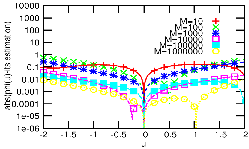
Figure 1: Relationship between the argument of the cumulant generating function when the demand $D_{a}$ is i.i.d. with a standard normalized distribution, with $L=1$ and $\left|\phi(u)-\log\left(\frac{1}{M}\sum_{a=1}^{M}e^{uD_{a}}\right)\right|$. The horizontal axis shows $u$, and the vertical axis shows the absolute difference between the cumulant generating function $\phi(u)$ and its estimate as $\log\left(\frac{1}{M}\sum_{a=1}^{M}e^{uD_{a}}\right)$, that is, $\left|\phi(u)-\log\left(\frac{1}{M}\sum_{a=1}^{M}e^{uD_{a}}\right)\right|$. When $M$ is large, $\log\left(\frac{1}{M}\sum_{a=1}^{M}e^{uD_{a}}\right)$ is close to the cumulant generating function $\phi(u)$. Moreover, it can be verified that this result has the self-averaging property [17, 18].

3 Analytic Results and Numerical Experiments

In this section, we verify the effectiveness of our proposed method using several examples of a multidimensional normal distribution, which can be used to model correlated commodities for which the statistical properties are well known.

3.1 Single commodity with i.i.d. normal distribution

First, we define the difference of the demand at $t$, $D_{t}$, of a single commodity over lead time $L$ from the mean $\mu=E[D_{t}]$ as $X_{t}(=D_{t}-\mu)$; we assume that the novel variable $X_{t}$ is i.i.d. with the normal distribution with mean $E[X_{t}]=0$ and variance $E[X_{t}^{2}]=\sigma^{2}$. From this, we have $\phi(u)=\frac{\sigma^{2}u^{2}}{2}$ when the safety stock quantity is $L\varepsilon$, and we obtain

$$Pr\left[L\varepsilon\leq X\right] = \int_{L\varepsilon}^{\infty}dXp(X)$$ (30)

$$\leq e^{-L\left(\frac{\varepsilon^{2}}{2\sigma^{2}}\right),}$$

where $X=\sum_{t=1}^{L}X_{t}=\sum_{t=1}^{L}D_{t}-L\mu$. From this, when the allowable stockout rate is $\delta$, the safety stock quantity is $L\varepsilon=\sqrt{-2L\sigma^{2}\log\delta}$.

One point should be noted here. In the case of the normal distribution, since the cumulant generating function $\phi(u)=\frac{\sigma^{2}u^{2}}{2}$ is already known, although the variance $\sigma^{2}$ appears in the safety stock quantity obtained from the above discussion, with respect to the demand distribution in general, the variance does not always appear in the description of the cumulant generation function, and it is not possible to determine a safety stock quantity for the general case that can guarantee a more adequate level of stockout rate. In a way similar to that shown in Fig. 1, if we can estimate the cumulant generating function, we can use the rate function to more accurately determine the safety stock quantity; this practical stock management strategy uses our proposed method.

Moreover, note that for this model, $Pr[L\varepsilon\leq X]$ can be obtained directly, as follows:

$$Pr\left[L\varepsilon\leq X\right]=H\left(\frac{L\varepsilon}{\sqrt{L\sigma^{2}}}\right),$$ (31)

where

$$H(k) = \int_{k}^{\infty}\frac{dt}{\sqrt{2\pi}}e^{-\frac{t^{2}}{2}}.$$ (32)

From this and Eq. (31), when the allowable stockout rate is $\delta$, the safety stock quantity $L\varepsilon(=SS_{\rm pre.})$ is

$$SS_{\rm pre.} = \sqrt{L\sigma^{2}}H^{-1}(\delta),$$ (33)

where $k=H^{-1}(\delta)$ is the inverse function of $H(k)=\delta$. It can be seen that the previous stock management strategy is a special case of our proposed method.

Two points should be noted here. First, although we analytically derive the safety stock quantity for the case of a normal distribution, analyze the Chernoff inequality in Eq. (30), and rigorously describe Eq. (31), it is not always easy to analytically solve for the stockout rate $Pr[L\varepsilon\leq X]$. Next, in general, even if the probability density function, $P(X_{t})$, of the demand difference from its mean, $X_{t}$, is well known, a rigorous allowable stockout rate $Pr[L\varepsilon\leq X]=E[\Theta(\sum_{t=1}^{L}X_{t}-L\varepsilon)]$ is analytically described as follows:

$$Pr[L\varepsilon\leq X]$$ (34)

$$= \int_{-\infty}^{\infty}\prod_{t=1}^{L}dX_{t}P(X_{t})\Theta\left(\sum_{t=1}^{L}X_{t}-L\varepsilon\right)$$

$$= \int_{-\infty}^{\infty}\prod_{t=2}^{L}dX_{t}P(X_{t})$$

$$\qquad\times\int_{{L\varepsilon-\sum_{t=2}^{L}X_{t}}}^{\infty}dX_{1}P(X_{1}).\qquad$$

However, even if we are able to find a closed form for the integral of $X_{1}$ in Eq. (34), the integrals of $X_{2},\cdots,X_{L}$ are not easy to evaluate, and we need to approximate this convolution integral, such as by using trapezoidal integration. In particular, since it is necessary to compute the exponential of $L-1$, it cannot be rigorously evaluated. On the other hand, if we can examine the moment-generating function using the approach based on Chernoff inequality, then we can assess the rate function $R(\varepsilon)$ and the safety stock quantity $L\varepsilon$ corresponding to the allowable stockout rate.

3.2 Definition of stockout rate

In this subsection, we summarize our method for management of the safety stock of multiple commodities. For simplicity, we will consider the case of two types of commodities. For a lead time $L$, let $X_{t}$ and $Y_{t}$ be the normalized demands (that is, the difference between current demand and mean demand) of two commodities, respectively. We assume that $X_{t},Y_{t}$ are i.i.d. with the Gaussian distribution such that $E[X_{t}]=E[Y_{t}]=0$, $E[X_{t}^{2}]=\sigma_{X}^{2}$, $E[Y_{t}^{2}]=\sigma_{Y}^{2}$, and $E[X_{t}Y_{t}]=\rho\sigma_{X}\sigma_{Y}$. From this, the probabilities that the sums of demand over lead time $L$, $X=\sum_{t=1}^{L}X_{t}$ and $Y=\sum_{t=1}^{L}Y_{t}$, exceed $L\varepsilon_{X}$ and $L\varepsilon_{Y}$, respectively, are calculated as follows:

$$Pr[L\varepsilon_{X}\leq X] = H\left(\frac{L\varepsilon_{X}}{\sqrt{L\sigma^{2}_{X}}}\right),$$ (35)

$$Pr[L\varepsilon_{Y}\leq Y] = H\left(\frac{L\varepsilon_{Y}}{\sqrt{L\sigma^{2}_{Y}}}\right).$$ (36)

In addition, it is also necessary to evaluate the stockout probability: $Pr[L\varepsilon_{X}\leq X,L\varepsilon_{Y}\leq Y]$ and $Pr[L\varepsilon_{X}\leq X,L\varepsilon_{Y}\leq Y]+Pr[L\varepsilon_{X}>X,L\varepsilon_{Y}\leq Y]+Pr[L\varepsilon_{X}\leq X,L\varepsilon_{Y}>Y]$ in the case of more than three commodities. Since the variation of these states of stockout is exponentially increasing with the number of commodities, and from the discussion in subsection 2.2, the Chernoff inequality holds for any pattern of stockout. Hereafter, we will discuss just one of the stockout patterns, the case of all commodities are stockout.

3.3 Two commodities that are i.i.d. with normal distribution

Let the demands of commodities 1 and 2 be $D_{t}^{X}$ and $D_{t}^{Y}$, respectively. Differences from the demand and its average demand over the lead time ($E[D_{t}^{X}]=\mu_{X},E[D_{t}^{Y}]=\mu_{Y}$) are represented as $X_{t}=D_{t}^{X}-\mu_{X},Y_{t}=D_{t}^{Y}-\mu_{Y}$, $E[X_{t}]=E[Y_{t}]=0$, $E[X_{t}^{2}]=\sigma_{X}^{2},E[Y_{t}^{2}]=\sigma_{Y}^{2}$, and $E[X_{t}Y_{t}]=E[X_{t}]E[Y_{t}]=0$. From this, when the respective safety stock quantities are $L\varepsilon_{X}$ and $L\varepsilon_{Y}$ over lead time $L$, the stockout rate $Pr[L\varepsilon_{X}\leq X,L\varepsilon_{Y}\leq Y]$, which is the probability that both commodities are missing simultaneously, is

$$Pr\left[L\varepsilon_{X}\leq X,L\varepsilon_{Y}\leq Y\right]$$ (37)

$$= \int_{L\varepsilon_{X}}^{\infty}dX\int_{L\varepsilon_{Y}}^{\infty}dYp(X,Y)$$

$$\leq e^{-L\left(\frac{\varepsilon_{X}^{2}}{2\sigma^{2}_{X}}+\frac{\varepsilon_{Y}^{2}}{2\sigma^{2}_{Y}}\right)},$$

where $X=\sum_{t=1}^{L}X_{t}$ and $Y=\sum_{t=1}^{L}Y_{t}$. From this, the allowable stockout rate when the safety stock quantities $L\varepsilon_{X},L\varepsilon_{Y}$ are $L\varepsilon_{X}=\sqrt{2L\sigma_{X}^{2}\log(1/\delta_{X})},L\varepsilon_{Y}=\sqrt{2L\sigma_{Y}^{2}\log(1/\delta_{Y})}$ is $\delta=\delta_{X}\delta_{Y}$. Moreover, $Pr[L\varepsilon_{X}\leq X,L\varepsilon_{Y}\leq Y]$ can be directly evaluated as follows:

$$Pr\left[L\varepsilon_{X}\leq X,L\varepsilon_{Y}\leq Y\right]$$ (38)

$$= H\left(\frac{L\varepsilon_{X}}{\sqrt{L\sigma^{2}_{X}}}\right)H\left(\frac{L\varepsilon_{Y}}{\sqrt{L\sigma^{2}_{Y}}}\right).$$

From this, if we have

$$L\varepsilon_{X} = \sqrt{L\sigma^{2}_{X}}H^{-1}\left(\delta_{X}\right),$$ (39)

$$L\varepsilon_{Y} = \sqrt{L\sigma^{2}_{Y}}H^{-1}\left(\delta_{Y}\right),$$ (40)

then the allowable stockout rate $\delta=\delta_{X}\delta_{Y}$ is obtained.

3.4 Two normally distributed, correlated commodities

Let $X_{t},Y_{t}$ be the demands of two correlated commodities over lead time $L$, where they are normally distributed with mean $E[X_{t}]=E[Y_{t}]=0$, variance $E[X_{t}^{2}]=\sigma_{X}^{2}$, $E[Y_{t}^{2}]=\sigma_{Y}^{2}$, and covariance $E[X_{t}Y_{t}]={\rho}\sigma_{X}\sigma_{Y}$. Then, when the safety stock quantities are $L\varepsilon_{X}$ and $L\varepsilon_{Y}$, the stockout rate $Pr[L\varepsilon_{X}\leq X,L\varepsilon_{Y}\leq Y]$ is

$$Pr\left[L\varepsilon_{X}\leq X,L\varepsilon_{Y}\leq Y\right]$$ (41)

$$= \int_{L\varepsilon_{X}}^{\infty}dX\int_{L\varepsilon_{Y}}^{\infty}dYp(X,Y)$$

$$\leq \exp\left[-\frac{L\left(\frac{\varepsilon_{X}^{2}}{\sigma^{2}_{X}}-2\rho\frac{\varepsilon_{X}\varepsilon_{Y}}{\sigma_{X}\sigma_{Y}}+\frac{\varepsilon_{Y}^{2}}{\sigma_{Y}^{2}}\right)}{2(1-\rho^{2})}\right],$$

where $X=\sum_{t=1}^{L}X_{t}$ and $Y=\sum_{t=1}^{L}Y_{t}$. From this,

$$L\varepsilon_{X} = \sqrt{-2L\sigma_{X}^{2}\log\delta_{X}},$$ (42)

$$L\varepsilon_{Y} = \frac{\sigma_{Y}}{\sigma_{X}}\rho(L\varepsilon_{X})+\sqrt{-2L\sigma_{Y}^{2}(1-\rho^{2})\log\delta_{Y}},$$ (43)

and thus we can evaluate $\delta=\delta_{X}\delta_{Y}$. Note that in this model, $Pr[L\varepsilon_{X}\leq X,L\varepsilon_{Y}\leq Y]$ is directly calculated as a double integral:

$$Pr\left[L\varepsilon_{X}\leq X,L\varepsilon_{Y}\leq Y\right]$$ (44)

$$= \int_{\frac{L\varepsilon_{X}}{\sqrt{L\sigma_{X}^{2}}}}^{\infty}\frac{du}{\sqrt{2\pi}}e^{-\frac{u^{2}}{2}}$$

$$\times H\left(\frac{1}{\sqrt{1-\rho^{2}}}\left(\frac{L\varepsilon_{Y}}{\sqrt{L\sigma^{2}_{Y}}}-\rho u\right)\right),\qquad$$

where, if $\rho=0$, Eq. (44) matches Eq. (38). In this case, we have another analytic description of the stockout rate:

$$Pr[L\varepsilon_{X}\leq X,L\varepsilon_{Y}\leq Y]$$ (45)

$$= \int_{\frac{L\varepsilon_{X}}{\sqrt{L\sigma_{X}^{2}(1-\rho^{2})}}}^{\infty}ds\int_{\frac{L\varepsilon_{Y}}{\sqrt{L\sigma_{Y}^{2}(1-\rho^{2})}}}^{\infty}dt\frac{1}{{2\pi}}e^{-\frac{s^{2}+t^{2}}{2}}$$

$$e^{\rho st}\sqrt{1-\rho^{2}}.\qquad$$

As in the discussion of Eq. (34), as the lead time $L$ increases, the calculation amount increases exponentially with the number of items to be considered ($N$), so for a sufficiently large $N$, it is not practical to use a direct method, such as Eq. (44) or (45).

3.5 Numerical experiments

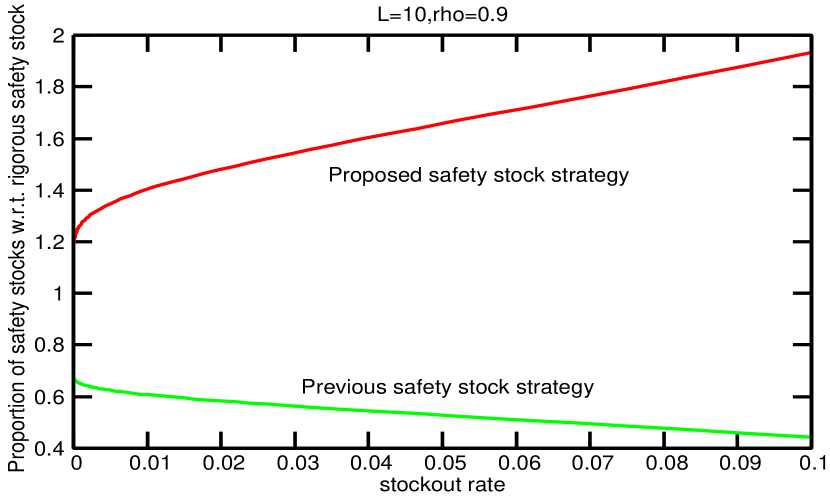
Figure 2: Comparison between the safety stock quantity derived by our proposed method $SS_{\rm pro.}$ relative to the rigorous safety stock $SS_{\rm rig.}$ and the safety stock quantity estimated by the previous method $SS_{\rm pre.}$ relative to the rigorous safety stock $SS_{\rm rig.}$. The horizontal axis shows the allowable stockout rate $\delta$ and the vertical axis shows the safety stock rate.

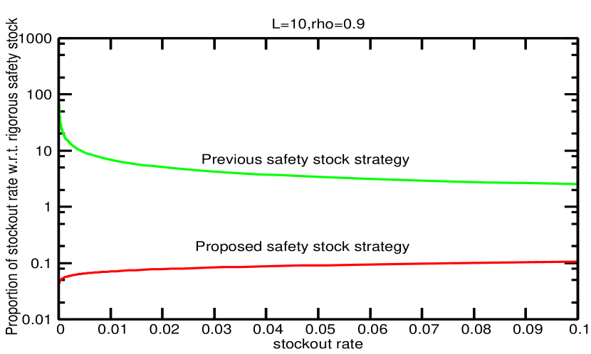
Figure 3: Comparison between the proportion of the stockout rate by our proposed method with respect to the allowable stockout rate ${\cal P}(SS_{\rm pro.})/{\cal P}(SS_{\rm rig.})$ and theproportion of the stockout rate by the previous method with respect to the allowable stockout rate ${\cal P}(SS_{\rm pre.})/{\cal P}(SS_{\rm rig.})$. The horizontal axis shows the allowable stockout rate $\delta$ and the vertical axis shows the proportionss of the stockout rate with respect to allowable stockout rate.

In this subsection, we evaluate the effectiveness of the proposed method by conducting numerical experiments. For simplicity, we consider the case in which the demands have equal variance, $\sigma_{X}^{2}=\sigma_{Y}^{2}=\sigma^{2}$. From this symmetry, we can evaluate $\delta_{X},\delta_{Y}$ by assuming $L\varepsilon_{X}=L\varepsilon_{Y}=L\varepsilon$. From Eqs. (39), (40), (42), (43) and (45), for a given allowable stockout rate $\delta$, the rigorous safety stock quantity $SS_{\rm rig.}$ (rig.=rigorous), the proposed safety stock quantity $SS_{\rm pro.}$ (pro.=proposed), and the previous safety stock quantity $SS_{\rm pre.}$ (pre.=previous) can be evaluated:

$$SS_{\rm rig.} = {\cal P}^{-1}(\delta),$$ (46)

$$SS_{\rm pro.} = \sqrt{{L}\sigma^{2}({1+\rho})\log(1/\delta)},$$ (47)

$$SS_{\rm pre.} = \sqrt{L\sigma^{2}}H^{-1}(\sqrt{\delta}),$$ (48)

where we use the inverse function of ${\cal P}(SS)=Pr[SS\leq X,SS\leq Y]$ defined in Eqs. (44) and (45). Furthermore, from subsection 3.3, we have $\delta_{X}=\delta_{Y}=\sqrt{\delta}$, and from subsection 3.4, we have $\delta_{X}=\delta^{\frac{1+\rho}{2}},\delta_{Y}=\delta^{\frac{1-\rho}{2}}$.

Fig. 2 compares the proportion of the proposed safety stock quantity with respect to the rigorous safety stock quantity $SS_{\rm pro.}/SS_{\rm rig.}$ and the proportion of the previous safety stock quantity with respect to the rigorous safety stock quantity $SS_{\rm pre.}/SS_{\rm rig.}$. Similarly, the proportions of the stockout rates ${\cal P}(SS_{\rm pro.})/{\cal P}(SS_{\rm rig.})$ and ${\cal P}(SS_{\rm pre.})/{\cal P}(SS_{\rm rig.})$ are indicated in Fig. 3. In Figs. 2 and 3, $\sigma^{2}=1$, $\rho=0.9$, $L=10$. From Fig. 2, it can be seen that when the allowable stockout rate is less than $10\%$, the safety stock quantity derived from the proposed method is 1.2 to 1.9 times the rigorous safety stock quantity. From Fig. 3, it can be seen that the stockout rate of the proposed method is always less than the allowable stockout rate; this is guaranteed by the Chernoff inequality. However, with the existing method, the stockout rate always exceeds the allowable value. In addition, the other cases of $\rho,L$ used in Figs. 2 and 3 are also guaranteed. Thus, it is clear that despite the safety stock, which is meant to minimize the opportunity loss, when there is a correlation between the different types of commodities, the proper level cannot be guaranteed by the previous method.

4 Conclusion and future work

In this study, we proposed a novel method for stock management of multiple commodities with correlated demands; we used the Chernoff inequality to derive the relation between the safety stock quantity and the allowable shortage rate. Using the rate function defined by Legendre’s transformation of the cumulant generating function, we were able to determine the safety stock level that would ensure that the stockout rate would always be acceptable. The theoretical properties are well known, since they follow a multidimensional normal distribution. We derived the safety stock for three different models: our proposed method, an existing method, and the exact (analytical) method. We determined the allowable stockout rate for each, and we verified the effectiveness of our method by conducting numerical experiments.

In this study, we considered two correlated commodities, but in order to increase the usefulness of the proposed method, we discussed the safety stock amount for multiple commodities, including those with positive and negative correlations. We discussed the safety stock amount for one lifecycle, but in reality, it is important to consider the safety stock while including preorders and back orders and spanning multiple life cycles. We intend to address this in our future research.

Appendix A Properties of the rate function

In this appendix, we present the properties of the rate function $R(\eta)$, which is used to derive the relation between the safety stock quantity and the allowable stockout rate. First, we can rewrite Eq. (11), the definition of the rate function, as follows:

$$R(u,\eta) = u\eta-\log E[e^{uD}],$$ (49)

where $R(0,\eta)=0$, and $R(u,\eta)$ is a continuous function of $u$, and so

$$R(\eta) \geq 0.$$ (50)

Thus, we obtain a positive upper bound for $Pr[\eta\leq D]$ by using the Chernoff inequality: $Pr[\eta\leq D]\leq e^{-R(\eta)}\leq e^{-0}=1$.

Next, since the exponential function is convex, $E[e^{uD}]\geq e^{uE[D]}$ holds, and so we obtain

$$R(u,\eta) \leq u\eta-uE[D].$$ (51)

When $\eta\leq E[D]$, since $u(\eta-E[D])\leq 0$, the optimal value for $u$ is close to $0$, and we obtain $R(\eta)=0$. On the other hand, when $\eta\geq E[D]$, the optimal value for $u$ is not equal to $0$, and so we obtain $R(\eta)>0$. Thus, we can rewrite the definition for $\eta$ as $\eta=E[D]+\varepsilon$, and it can be seen that the sign of the rate function is determined by the sign of $\varepsilon$, that is, if $\varepsilon\leq 0$, then $R(\eta)=0$, otherwise, $R(\varepsilon)>0$. Hereafter, we will consider the rate function $R(\eta)$ to be a function of the distance from the mean, $E[D]$.

We also note that, from the definition of the rate function, $R(u,\eta)$ is convex with respect to $u$, since $\frac{\partial^{2}R(u,\eta)}{\partial u^{2}}\leq 0$. Thus, the following updating rule will optimize $u$:

$$u_{s+1} = u_{s}+\kappa_{u}\lim_{u\to u_{s}}\frac{\partial R(u,\eta)}{\partial u},$$ (52)

where $u_{s}$ is the state of $u$ at step $s$, for $s\in{\bf Z}$, and the step constant is $\kappa_{u}=10^{-3}$. This iterative definition ceases if $|u_{s}-u_{s+1}|$ is close to $0$ or the variation of $u$ is smaller than an infinitesimal $\theta$, such as $\theta=10^{-6}$. Both the control parameter $u$ and the constant $\eta$ can develop to represent a multidimensional case; for instance, for $\vec{u},\vec{\eta}\in{\bf R}^{N}$, $R(\vec{u},\vec{\eta})$ is convex with respect to $\vec{u}$, and thus $R(\vec{\eta})=\mathop{\max}_{\vec{u}}R(\vec{u},\vec{\eta})$ is concave with respect to $\vec{\eta}$. From the above conclusions, and using the convexity of the rate function, the duality of the rate function and the cumulant generating function, and an algorithm developed in convex optimization research, we can assess a more appropriate safety stock quantity for stock management under stochastic phenomena.

Appendix B Availability of Eq. (11)

Eq. (11) shows the Chernoff inequality with respect to $N$ commodities. The normalized demand (or the difference between current demand and mean demand) over lead time $L$, $X_{it},(i=1,\cdots,N,t=1,\cdots,L)$, is not temporally correlated and follows the normal distribution with $E[X_{it}]=0,E[X_{it}X_{jt}]=\Sigma_{ij}$. From Eq. (11), we can derive the following inequality:

$$Pr\left[L\vec{\varepsilon}\leq\vec{X}\right] \leq e^{-L\vec{u}^{\rm T}\vec{\varepsilon}+\frac{L}{2}\vec{u}^{\rm T}\Sigma\vec{u}},$$ (53)

where $\vec{u}\geq 0$, $\vec{X}=\sum_{t=1}^{L}\vec{X}_{t}$, and the variance-covariance matrix $\Sigma=\left\{\Sigma_{ij}\right\}\in{\bf R}^{N\times N}$. We can obtain a tighter upper bound by using the following equation with respect to the parameter $\vec{u}$:

$$\vec{u}_{s+1} = \max\left(\vec{u}_{s}+\kappa(\vec{\varepsilon}-\Sigma\vec{u}_{s}),0\right),$$ (54)

where $\kappa$ is positive and infinitesimal, $\vec{u}_{0}=(1,1,\cdots,1)^{\rm T}\in{\bf R}^{N}$, and at step $s$, $\vec{u}_{s}=(u_{1,s},\cdots,u_{N,s})^{\rm T}\in{\bf R}^{N}$. The stopping condition is $\Delta=\sum_{i=1}^{L}\left|u_{i,s+1}-u_{i,s}\right|<10^{-6}$. The rigorous stockout rate $L\vec{\varepsilon}$ is calculated as follows:

$$Pr\left[L\vec{\varepsilon}\leq\vec{X}\right] = \int_{L\vec{\varepsilon}}^{\infty}\frac{d\vec{X}e^{-\frac{1}{2L}\vec{X}^{\rm T}\Sigma^{-1}\vec{X}}}{(2\pi)^{\frac{N}{2}}\sqrt{\det(L\Sigma)}}.\qquad$$ (55)

We first diagonalize the variance covariance matrix $\Sigma$, and then we prepare the novel variables, which are in the directions of the eigenvectors of $\Sigma$. However, since the integral domain of the novel variables is more complicated, it is not easy to analytically assess the right-hand side of Eq. (55). Thus, we use trapezoidal integration to approximate it when the number of commodities, $N$, is large; however, the computational complexity increases exponentially with $N$, so this approach is not practical.

Appendix C Safety stock management for fungible commodities

We here discuss the safety stock management for the case in which $X$ and $Y$ are fungible commodities. Using the model setting in subsection 3.4, with respect to the modified demands for two commodities $X$ and $Y$ over lead time $L$, where we consider their differences from their means, $X_{t},Y_{t}$ (since they are fungible, we assume that they have a negative correlation), the probability that the sum $\sum_{t=1}^{L}X_{t}+\sum_{t=1}^{L}Y_{t}$ is larger than the safety stock quantity $L\varepsilon$ is calculated using the Chernoff inequality:

$$Pr\left[L\varepsilon\leq\sum_{t=1}^{L}(X_{t}+Y_{t})\right]$$ (56)

$$\leq e^{-uL\varepsilon}E\left[e^{u\sum_{t=1}^{L}(X_{t}+Y_{t})}\right]$$

$$= e^{-uL\varepsilon+\frac{Lu^{2}}{2}(\sigma_{X}^{2}+\sigma_{Y}^{2}+2\rho\sigma_{X}\sigma_{Y})}.$$

From this, the rate function is

$$R(\varepsilon) = \mathop{\max}_{u>0}\left\{u\varepsilon-\frac{u^{2}}{2}(\sigma_{X}^{2}+\sigma_{Y}^{2}+2\rho\sigma_{X}\sigma_{Y})\right\}$$ (57)

$$= \frac{\varepsilon^{2}}{2(\sigma_{X}^{2}+\sigma_{Y}^{2}+2\rho\sigma_{X}\sigma_{Y})}.$$

Thus, the safety stock with respect to the allowable stockout rate $\delta$ is

$$L\varepsilon = \sqrt{-2L(\sigma_{X}^{2}+\sigma_{Y}^{2}+2\rho\sigma_{X}\sigma_{Y})\log\delta}.$$ (58)

Here, we assume that the correlation between $X$ and $Y$ is negative, but this also applies when the correlation is positive. Thus, the safety stock quantity $L\varepsilon$ is a monotonically nondecreasing function with respect to the correlation coefficient $\rho$.

References

•  1. Fotopoulos S., Wang M.-C., Rao S. S., 1988. Safety stock determination with correlated demands and arbitrary lead times, European Journal of Operations Research, 35(2), 172-181.
•  2. Takemoto Y., Iwamoto I., Arizono I., 2011. Proposal of reorder point satisfying allowable shortage rate under limited demand information, Journal of Japan Industrial Management Association, 62(1), 21-24.
•  3. Arizono I., Takemoto Y., 2013. A proposal for setting electric power saving rate to avoid risk of electric power shortage occurrence, Synthesiology, 6(3), 140-151.
•  4. Shinzato T., Kaku I., 2011. Large deviation approach for safety stock management for correlated demands, Journal of Japan Industrial Management Association, 62(4), 164-173.
•  5. Schmidt J. P., Siegel A., Srinivasan A., 1995. Chernoff-Hoeffding bounds for applications with limited independence, SIAM Journal on Discrete Mathematics, 8(2), 223-250.
•  6. Silver E. A., Pyke D. F., Peterson R., 1998. Inventory management and production planning and scheduling, Wiley.
•  7. Kottas J. K., Lau H. S., 1979. A realistic approach for modeling stochastic laed time distributions, AIIE Transactions, 11(1), 54-60.
•  8. Kottas J. K., Lau H. S., 1980. The use of versatile distribution families in some stochastic inventory calculations, Journal of the Operational Research Society, 31(5), 393-403.
•  9. Ray W. D., 1980. The significance of correlated demands and variable lead time for stock control policies, Journal of the Operational Research Society, 31(2), 187-190.
•  10. Ray W. D., 1981. Computation of reorder level when the demands are correlated and the lead time random, Journal of the Operational Research Society, 32(1), 27-34.
•  11. Bagchi U., Hayya J. C., Ord J. K., 1983. The Hermite distribution as a model of demand during lead time for slow-moving items, Decision Sciences, 14(4), 447-466.
•  12. Bagchi U., Hayya J. C., Ord J. K., 1983. The distribution of demand during lead time, A synthesis of the state of the use art, working paper, Pennsylvania state university.
•  13. Van Ness P. D., Stevenson N. J., 1983. Reorder-point models with discrete probability distributions, Decision Sciences, 14(3), 363-369.
•  14. Lau H. S., Wang M. C., 1987. Estimating the lead-time demand distribution when the daily demand is non-normal and autocorrelated, European Journal of Operations Research, 29(1), 60-67.
•  15. Zang R., Kaku I., Xiao Y., 2011. Deterministic EOQ with partial backordring and correlated demand caused by cross-selling, European Journal of Operations Research, 201(3), 537-551.
•  16. Cengel Y. A., Boles M. A., 2010. Thermodynamics: An engineering approach, McGraw Hill Higher Education.
•  17. Shinzato T., 2015. Self-Averaging Property of Minimal Investment Risk of Mean-Variance Model, Public Library of Science One, 10(7), e0133846.
•  18. Wakai R., Shinzato T., Shimazaki Y., 2014. Random matrix appproach for portfolio optimization problem, Journal of Japan Industrial Management Association, 65(1), 17-28.