$k^{\tau,\epsilon}$-anonymity: Towards Privacy-Preserving Publishing of Spatiotemporal Trajectory Data

Abstract

Mobile network operators can track subscribers via passive or active monitoring of device locations. The recorded trajectories offer an unprecedented outlook on the activities of large user populations, which enables developing new networking solutions and services, and scaling up studies across research disciplines. Yet, the disclosure of individual trajectories raises significant privacy concerns: thus, these data are often protected by restrictive non-disclosure agreements that limit their availability and impede potential usages. In this paper, we contribute to the development of technical solutions to the problem of privacy-preserving publishing of spatiotemporal trajectories of mobile subscribers. We propose an algorithm that generalizes the data so that they satisfy $k^{\tau,\epsilon}$-anonymity, an original privacy criterion that thwarts attacks on trajectories. Evaluations with real-world datasets demonstrate that our algorithm attains its objective while retaining a substantial level of accuracy in the data. Our work is a step forward in the direction of open, privacy-preserving datasets of spatiotemporal trajectories.

I Introduction

Subscriber trajectory datasets collected by network operators are logs of timestamped, georeferenced events associated to the communication activities of individuals. The analysis of these datasets allows inferring fine-grained information about the movements, habits and undertakings of vast user populations. This has many different applications, encompassing both business and research. For instance, trajectory data can be used to devise novel data-driven network optimization techniques [1] or support content delivery operations at the network edge [2]. They can also be monetized via added-value services such as transport analytics [3] or location-based marketing [4]. Additionally, the relevance of massive movement data from mobile subscribers is critical in research disciplines such as physics, sociology or epidemiology [5].

The importance of trajectory data has also been recognized in the design of future 5G networks, with a thrust towards the introduction of data interfaces among network operators and over-the-top (OTT) providers to give them online access to this (and other) data. OTTs can leverage such interfaces to automatically retrieve the data and process them on the fly, thus enabling new applications such as intelligent transportation [6] or assisted-life services [7].

All these use cases stem from the disclosure of trajectory datasets to third parties. However, the open release of such data is still largely withhold, which hinders potential usages and applications. A major barrier in this sense are privacy concerns: data circulation exposes it to re-identification attacks, and cognition of the movement patterns of de-anonymized individuals may reveal sensitive information about them.

This calls for anonymization techniques. The common practice operators adhere to is replacing personal identifiers (e.g., name, phone number, IMSI) with pseudo-identifiers (i.e., random or non-reversible hash values). Whether this is a sufficient measure is often called into question, especially in relation to the possibility of tracking user movements. What is sure is that pseudo-identifiers have been repeatedly proven not to protect against user trajectory uniqueness, i.e., the fact that mobile subscribers have distinctive travel patterns that make them univocally recognizable even in very large populations [8, 9, 10]. Uniqueness is not a privacy threat per-se, but it is a vulnerability that can lead to re-identification. Examples are brought forth by recent attempts at cross-correlating mobile operator-collected trajectories with georeferenced check-ins of Flickr and Twitter users [11], with credit card records [12] or with Yelp, Google Places and Facebook metadata [13].

More dependable anonymization solutions are needed. However, the strategies devised to date for relational databases, location-based services, or regularly sampled (e.g., GPS) mobility do not suit the irregular sampling, time sparsity, and long duration of trajectories collected by mobile operators. Moreover, current privacy criteria, including $k$-anonymity and differential privacy, do not provide sufficient protection or are impractical in this context. See Sec. V for a detailed discussion.

In this paper, we put forward several contributions towards privacy-preserving data publishing (PPDP) of mobile subscriber trajectories. Our contributions are as follows: (i) we outline attacks that are especially relevant to datasets of spatiotemporal trajectories; (ii) we introduce $k^{\tau,\epsilon}$-anonymity, a novel privacy criterion that effectively copes with the most threatening attacks above; (iii) we develop k-merge, an algorithm that solves a fundamental problem in the anonymization of spatiotemporal trajectories, i.e., effective generalization; (iv) we implement kte-hide, a practical solution based on k-merge that attains $k^{\tau,\epsilon}$-anonymity in spatiotemporal trajectory data; (v) we evaluate our approach on real-world datasets, showing that it achieves its objectives while retaining a substantial level of accuracy in the anonymized data.

II Requirements and models

We first present the requirements of PPDP, in Sec. II-A, and formalize the specific attacker model we consider, in Sec. II-B. We then propose a consistent privacy model, in Sec. II-C.

II-A PPDP requirements

PPDP is defined as the development of methods for the publication of information that allows meaningful knowledge discovery, and yet preserves the privacy of monitored subjects [14]. The requisites of PPDP are similar for all types of databases, including our specific case, i.e., datasets of spatiotemporal trajectories. They are as follows.

• The non-expert data publisher. Mining of the data is performed by the data recipient, and not by the data publisher. The only task of the data publisher is to anonymize the data for publication.

• Publication of data, and not of data mining results. The aim of PPDP is producing privacy-preserving datasets, and not anonymized datasets of classifiers, association rules, or aggregate statistics. This sets PPDP apart from privacy-preserving data mining (PPDM), where the final usage of the data is known at dataset compilation time.

• Truthfulness at the record level. Each record of the published database must correspond to a real-world subject. Moreover, all information on a subject must map to actual activities or features of the subject. This avoids that fictitious data introduces unpredictable biases in the anonymized datasets.

Our privacy model will obey the principles above. We stress that they impose that the privacy model must be agnostic of data usage (points 1 and 2), and that it cannot rely on randomized, perturbed, permuted and synthetic data (point 3).

II-B Attacker model

Unlike PPDP requirements, the attacker model is necessarily specific to the type of data we consider, and it is characterized by the knowledge and goal of the adversary. The former describes the information the opponent possesses, while the latter represents his privacy-threatening objective.

II-B1 Attacker knowledge

In trajectory datasets, each data record is a sequence of spatiotemporal samples. We assume an attacker who can track a target subscriber continuously during any amount of time $\tau$. The adversary knowledge consists then in all spatiotemporal samples in the victim’s trajectory over a continuous time interval of duration $\tau$.

II-B2 Attacker goal

Attacks against user privacy in published data can have different objectives, and a comprehensive classification is provided in [14]. Two classes of attacks are especially relevant in the context of mobile subscriber trajectory data. Both exploit the uniqueness of movement patterns that, as mentioned in Sec. I, characterizes trajectory data.

• Record linkage attacks. These attacks aim at univocally distinguishing an individual in the database. A successful record linkage enables cross-database correlation, which may ultimately unveil the identity of the user. Record linkage attacks on mobile traffic data have been repeatedly and successfully demonstrated [8, 9, 10]. As mentioned in Sec. I, they have also been used for subsequent cross-database correlations [11, 12, 13].

• Probabilistic attacks. These attacks let an adversary with partial information about an individual enlarge his knowledge on that individual by accessing the database. They are especially relevant to spatiotemporal trajectories, as shown by seminal works that first unveiled the anonymization issues of mobile traffic datasets [8, 9]. Let us imagine a scenario where an adversary knows a small set of spatiotemporal points in the trajectory of a subscriber (because, e.g., he met the target individual there). A successful probabilistic attack would reveal the complete movements of the subscriber to the attacker, who could then use them to infer sensitive information about the victim, such as home/work locations, daily routines, or visits to healthcare structures.

Our privacy model will address both classes of attacks above, led by an adversary with knowledge described in Sec. II-B1.

II-C Privacy model

Our privacy model is designed following the PPDP requirements and attacker model presented before. We start by considering suitable privacy criteria against record linkage and probabilistic attacks, in Sec. II-C1 and Sec. II-C2, respectively. We then show how the first criterion is in fact a specialization of the second, in Sec. II-C3, which allows us to focus on a single unifying privacy model. Finally, we present the elementary techniques that we employ to implement the target privacy criterion, in Sec. II-C4.

II-C1 $k$-anonymity

The $k$-anonymity criterion realizes the indistinguishability principle, by commending that each record in a database must be indistinguishable from at least $k-1$ other records in the same database [15]. In our case, this maps to ensuring that each subscriber is hidden in a crowd of $k$ users whose trajectories cannot be told apart. The popularity of $k$-anonymity for PPDP has led to indiscriminated use beyond its scope, and subsequent controversy on the privacy guarantees it can provide. E.g., $k$-anonymity has been proven ineffective againt attacks aiming at attribute linkage (including exploits of insufficient side-information diversity), at localizing users, or at disclosing their presence and meetings [16, 17, 18].

However, $k$-anonymity remains a legitimate criterion against record linkage attacks on any kind of database [14]. Therefore, this privacy model protects trajectory data from the first type of attack in Sec. II-B, including its variations in [8, 9, 10, 11, 12, 13].

II-C2 $k^{\tau,\epsilon}$-anonymity

No privacy criterion proposed to date can safeguard spatiotemporal trajectory data from the second type of attacks in Sec. II-B, i.e., probabilistic attacks. This forces us to define an original criterion, as follows.

The pertinent principle here is the so-called uninformative principle, i.e., ensuring that the difference between the knowledge of the adversary before and after accessing a database is small [16]. In our context, this principle warrants that an attacker who knows some subset of a subscriber’s movements cannot extract from the dataset a substantially longer portion of that user’s trajectory.

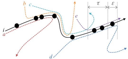
Figure 1: Illustrative example of $k^{\tau,\epsilon}$-anonymity of user $i$, with $k$=2.

To attain the uninformative principle, we introduce the $k^{\tau,\epsilon}$-anonymity privacy criterion. $k^{\tau,\epsilon}$-anonymity can be seen as a variation of $k^{m}$-anonymity, which establishes that each individual in a dataset must be indistinguishable from at least $k-1$ other users in the same dataset, when limiting the attacker knowledge to any set of $m$ attributes [19]. $k^{\tau,\epsilon}$-anonymity tailors $k^{m}$-anonymity to our scenario, as follows.

• As per Sec. II-B, the attacker knowledge can be any continued sequence of spatiotemporal samples covering a time interval of length at most $\tau$: thus, the $m$ parameter of $k^{m}$-anonymity maps to the (variable) set of samples contained in any time period $\tau$. During any such time period, every trajectory in the dataset must be indistinguishable from at least other $k-1$ trajectories.

• The maximum additional knowledge that the attacker is allowed to learn is called leakage; it consists of the spatiotemporal samples of the target user’s trajectory contained in a time interval of duration at most $\epsilon$, disjoint from the original $\tau$. In order to fulfill the uninformative principle, the leakage $\epsilon$ must be small.

The two requirements above imply alternating in time the $k-1$ trajectories that provide anonymization. An intuitive example is provided in Fig. 1. There, the trajectory of a target user $i$ is $2^{\tau,\epsilon}$-anonymized using those of five other subscribers. The overlapping between the trajectories of $a$, $b$, $c$, $d$, $e$ and that of $i$ is partial and varied. An adversary knowing a sub-trajectory of $i$ during any time interval of duration $\tau$ always finds at least one other user with a movement pattern that is identical to that of $i$ during that interval, but different elsewhere. With this knowledge, the adversary cannot tell apart $i$ from the other subscriber, and thus cannot attribute full trajectories to one user or the other. As this holds no matter where the knowledge interval is shifted to, the attacker can never retrieve the complete movement patterns of $i$: this achieves the uninformative principle. Still, the adversary can increase its knowledge in some cases. Let us consider the interval $\tau$ indicated in the figure: the trajectories of $i$, $d$ and $e$ are identical for some time after $\tau$, which allows associating to $i$ the movements during $\epsilon$: the opponent learns one additional spatiotemporal sample of $i$.

II-C3 Relationship between the privacy criteria

It is easy to see that $k$-anonymity is a special case of $k^{\tau,\epsilon}$-anonymity. As a matter of fact, the latter criterion reduces to the former when $\tau+\epsilon$ covers the whole temporal duration of the trajectory dataset. Then, $k^{\tau,\epsilon}$-anonymity commends that each complete trajectory is indistinguishable from $k-1$ other trajectories, which is the definition of $k$-anonymity. Our point here is that an anonymization solution that implements $k^{\tau,\epsilon}$-anonymity can be straightforwardly employed to attain $k$-anonymity as well, by properly adjusting the $\tau$ and $\epsilon$ parameters.

In the light of these considerations, we address the problem of achieving $k^{\tau,\epsilon}$-anonymity in datasets of spatiotemporal trajectories of mobile subscribers. By doing so, we develop a complete anonymization solution that is effective against probabilistic attacks, but can also be specialized to guarantee $k$-anonymity and counter record linkage attacks.

II-C4 Generalization and suppression

In order to enforce $k^{\tau,\epsilon}$-anonymity for all users in the dataset, we need to tweak the spatiotemporal samples in the trajectories of individuals, so that the criterion in Sec. II-C2 is respected for all of them. To that end, we rely on two elementary techniques, i.e., spatiotemporal generalization and suppression of samples.

Spatiotemporal generalization reduces the precision of trajectory samples in space and time, so as to make the samples of two or more users indistinguishable. Suppression removes from the trajectories those samples that are too hard to anonymize. Both techniques are lossy, i.e., imply some reduction of precision in the data. Yet, unlike other approaches, these techniques conform to the PPDP requirement of truthfulness at the record level, see Sec. II-A.

III Achieving $k^{\tau,\epsilon}$-anonymity

Our goal is ensuring that an anonymized dataset of mobile subscriber trajectories respects the uninformative principle, by implementing, through generalization and suppression, the $k^{\tau,\epsilon}$-anonymity of all subscriber trajectories in the dataset. Clearly, we aim at doing so while minimizing the loss of spatiotemporal granularity in the data.

We start by defining the basic operation of generalizing a set of spatiotemporal samples, and the associated cost in terms of loss of granularity, in Sec. III-A. We then extend both notions to (sub-)trajectories, in Sec. III-B. Building on these definitions, we discuss in Sec. III-C the optimal spatiotemporal generalization of $k$ (sub-)trajectories. We implement the result into k-merge, an optimal low-complexity algorithm that generalizes (sub-)trajectories with minimal loss of data granularity, in Sec. III-D. Once able to merge (sub-)trajectories optimally, we propose an approach to guarantee $k^{\tau,\epsilon}$-anonymity of the trajectory of a single user, in Sec. III-E, and we then scale the solution to multiple users in Sec. III-F. Finally, we introduce kte-hide, an algorithm that ensures $k^{\tau,\epsilon}$-anonymity in spatiotemporal trajectory datasets, in Sec. III-G.

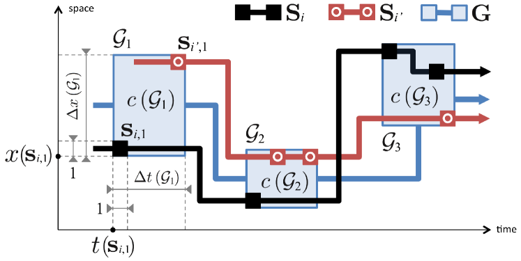
Figure 2: Example of merging of trajectories ${\bf S}_{i}=\{{\bf s}_{i,j}\}$ and ${\bf S}_{i^{\prime}}=\{{\bf s}_{i^{\prime},j}\}$ into a generalized trajectory ${\bf G}=\{{\cal G}\}$. For clarity, space is unidimensional.

III-A Generalization of samples

A (raw) sample of a spatiotemporal trajectory represents the position of a subscriber at a given time, and we model it with a length-3 real vector ${\bf s}=(t({\bf s}),x({\bf s}),y({\bf s}))$. Since a dataset is characterized by a finite granularity in time and space, a sample is in fact a slot spanning some minimum temporal and spatial intervals. The vector entries above can be regarded as the origins of a normalized length-1 time interval and a normalized 1$\times$1 two-dimensional area.

Spatiotemporal generalization merges together two or more raw samples into a generalized sample, i.e., a slot with a larger span. Mathematically, a generalized sample ${\cal G}$ can be represented as the set of the merged samples. There is a cost associated with merging samples, which is related to the span of the corresponding generalized sample, i.e., to the loss of granularity induced by the generalization. The cost of the operation of merging a set of samples into the generalized sample ${\cal G}$ is defined as

$$c\left({\cal G}\right)=c_{t}\left({\cal G}\right)c_{s}\left({\cal G}\right),$$ (1)

where $c_{t}\left({\cal G}\right)$ represents the cost in the time dimension, while $c_{s}\left({\cal G}\right)$ is the cost in the space dimensions.

Let ${\cal G}_{1}$ and ${\cal G}_{2}$ be two disjoint generalized samples (i.e., ${\cal G}_{1}\cap{\cal G}_{2}=\emptyset$). Then, we make the following two assumptions on the time and space merging costs:

$$c_{t}\left({\cal G}_{1}\cup{\cal G}_{2}\right)\geq c_{t}\left({\cal G}_{1}\right)+c_{t}\left({\cal G}_{2}\right)$$ (2)

$$c_{s}\left({\cal G}_{1}\cup{\cal G}_{2}\right)\geq\max\left\{c_{s}\left({\cal G}_{1}\right),c_{s}\left({\cal G}_{2}\right)\right\}.$$ (3)

Hereafter, we use the following definitions to implement the generic costs $c_{t}\left({\cal G}\right)$ and $c_{s}\left({\cal G}\right)$:

$$c_{t}\left({\cal G}\right)=\Delta t\left({\cal G}\right)$$ (4)

$$c_{s}\left({\cal G}\right)=\Delta x\left({\cal G}\right)+\Delta y\left({\cal G}\right),$$ (5)

where

$$\Delta\star\left({\cal G}\right)=\max_{{\bf s}\in{\cal G}}\hskip 2.0pt\star({\bf s})-\min_{{\bf s}\in{\cal G}}\hskip 2.0pt\star({\bf s})+1,$$ (6)

with $\star\in\{t,x,y\}$, is the span in each dimension.

Therefore, in our implementation, $c\left({\cal G}\right)$ is the area of a rectangle with sides $\Delta t\left({\cal G}\right)$ and $\Delta x\left({\cal G}\right)+\Delta y\left({\cal G}\right)$. A graphical example is provided in Fig. 2, where two raw samples ${\bf s}_{i,1}$ and ${\bf s}_{i^{\prime},1}$ are merged into a generalized sample ${\cal G}_{1}$, spanning $\Delta t({\cal G}_{1})$ in time and $\Delta x({\cal G}_{1})$ in space (portrayed as unidimensional in the figure, for the sake of readability).

Remark 1

The rationale for our choice of costs is computational efficiency. Also, summing the two space spans before multiplication allows balancing the time and space contributions. Finally, note that with the definition in (5), the space merging cost assumption in (3) is trivially true. Instead, the definition in (4) lets the time merging cost assumption in (2) hold only if the time intervals spanned by ${\cal G}_{1}$ and ${\cal G}_{2}$ are non-overlapping. The time coherence property that we will introduce in Sec. III-B ensures that this is the always case.

III-B Generalization of trajectories

A spatiotemporal (sub-)trajectory describes the movements of a single subscriber during the dataset timespan. Formally, a trajectory is an ordered vector of samples ${\bf S}=\left({\bf s}_{1},\dots,{\bf s}_{N}\right)$, where the ordering is induced by the time coordinate, i.e., $t({\bf s}_{i})<t({\bf s}_{i^{\prime}})$ if and only if $i<i^{\prime}$.

A generalized trajectory, obtained by merging different trajectories, is defined as an ordered vector of generalized samples ${\bf G}=\left({\cal G}_{1},\dots,{\cal G}_{Z}\right)$. Here the ordering is more subtle, and based on the fact that the time intervals spanned by the generalized samples are non-overlapping, a property that will be called time coherence. More precisely, if ${\cal G}_{i}$ and ${\cal G}_{i^{\prime}}$, $i<i^{\prime}$, are two generalized samples of ${\bf G}$, then

$$\max_{{\bf s}\in{\cal G}_{i}}t({\bf s})<\min_{{\bf s}\in{\cal G}_{i^{\prime}}}t({\bf s}).$$

An example of a generalized trajectory ${\bf G}$ merging two trajectories ${\bf S}_{i}$ and ${\bf S}_{i^{\prime}}$ is provided in Fig. 2. ${\bf G}$ fulfils time coherence, as its generalized samples are temporally disjoint.

Remark 2

Time coherence is a defining property of generalized trajectories in PPDP. As a matter of fact, publishing trajectory data with time-overlapping samples would generate semantic ambiguity and make analyses cumbersome.

Analogously to the cost of merging samples, we can define a cost of merging multiple trajectories into a generalized trajectory. We define such cost as the sum of costs of all generalized samples belonging to it. More precisely, if ${\bf G}=\left({\cal G}_{1},\dots,{\cal G}_{Z}\right)$, and $c(\cdot)$ is defined as in (1), then the cost of ${\bf G}$ is given by:

$$C\left({\bf G}\right)=\sum_{i=1}^{Z}c\left({\cal G}_{i}\right).$$ (7)

Remark 3

The cost in (7) is the overall surface covered by samples of the generalized trajectory over the spatiotemporal plane. E.g., in Fig. 2, the cost of ${\bf G}$ is the sum of the three areas, i.e., $c({\cal G}_{1})+c({\cal G}_{2})+c({\cal G}_{3})$. It is thus proportional to the total loss of granularity induced by the generalization.

III-C Optimal generalization of trajectories

We now formalize the problem of optimal generalization of spatiotemporal (sub-)trajectories. Suppose that we have $k$ trajectories ${\bf S}_{1},\dots,{\bf S}_{k}$, with ${\bf S}_{i}=({\bf s}_{i,1},\dots,{\bf s}_{i,N_{i}})$, $i=1,\dots,k$. The goal is a generalized trajectory ${\bf G}^{*}=\left({\cal G}^{*}_{1},\dots,{\cal G}^{*}_{Z}\right)$ from ${\bf S}_{1},\dots,{\bf S}_{k}$, which satisfies the following conditions.

i) The union of all generalized samples of ${\bf G}^{*}$ must coincide with the union of all samples of ${\bf S}_{1},\dots,{\bf S}_{k}$, i.e.,

$${\cal G}^{*}_{1}\cup\dots\cup{\cal G}^{*}_{Z}={\cal S}_{1}\cup\dots\cup{\cal S}_{k}\triangleq{\cal S},$$

where ${\cal S}_{i}=\bigcup_{j=1}^{N_{i}}\{{\bf s}_{i,j}\}$. Thus, ${\bf G}^{*}$ is a partition of the set ${\cal S}$ of all samples in the input trajectories: it does not add any alien sample or discard any input sample.

ii) Each generalized sample contains at least one sample from each of the $k$ input trajectories ${\bf S}_{1},\dots,{\bf S}_{k}$, i.e.,

$${\cal G}^{*}_{i}\cap{\cal S}_{i^{\prime}}\neq\emptyset,\,\,\,i=1,\dots,Z,\,\,\,i^{\prime}=1,\dots,k.$$

This imposes that each input trajectory contributes to each generalized sample of ${\bf G}^{*}$. Otherwise, the merging could associate generalized samples to users that never visited the generalized location at the generalized time, violating point 3 of the PPDP requirements in Sec. II-A.

iii) The cost of the merging is minimized, i.e.,

$${\bf G}^{*}=\mathop{\mathrm{arg~{}min}}\limits_{{\bf G}\in{\cal K}}C({\bf G}),$$ (8)

where ${\cal K}$ is the set of all partitions of ${\cal S}$ satisfying time coherence as well as condition ii) above, and $C({\bf G})$ is in (7). In Fig. 2, the generalized trajectory ${\bf G}$ fulfils all these requirements, and is thus the optimal merge ${\bf G}^{*}$ of ${\bf S}_{i}$ and ${\bf S}_{i^{\prime}}$.

Solving the problem above with a brute-force search is computationally prohibitive, since ${\cal K}$ has a size that grows exponentially with $|{\cal S}|/k$, where $|\cdot|$ denotes cardinality. However, we can characterize ${\bf G}^{*}$ so that it is possible to compute it with low complexity. To that end, we name elementary a partition ${\bf G}\in{\cal K}$ that cannot be refined to another partition within ${\cal K}$. In other words, none of the generalized samples of an elementary partition can be split into two generalized samples without violating conditions i) and ii) above, or time coherence. Then, we have the following proposition.

Proposition 1

Given the input trajectories ${\bf S}_{1},\dots,{\bf S}_{k}$, the optimal ${\bf G}^{*}$ defined in (8) is an elementary partition.

Proof: Suppose ${\bf G}\in{\cal K}$ is not elementary, so that it can be refined to another partition $\widetilde{{\bf G}}\in{\cal K}$. In particular, without loss of generality, suppose that ${\bf G}=({\cal G}_{1},\dots,{\cal G}_{Z})$ and $\widetilde{{\bf G}}=\left(\widetilde{{\cal G}}_{1},\dots,\widetilde{{\cal G}}_{Z+1}\right)$, where

$${\cal G}_{i}=\left\{\begin{array}[]{ll}\widetilde{{\cal G}}_{i},&i<Z\\ \widetilde{{\cal G}}_{Z}\cup\widetilde{{\cal G}}_{Z+1},&i=Z.\end{array}\right.$$ (9)

From (7) and (9), the difference between the costs of ${\bf G}$ and $\widetilde{{\bf G}}$ is given by

$$C({\bf G})-C(\widetilde{{\bf G}})=c({\cal G}_{Z})-c(\widetilde{{\cal G}}_{Z})-c(\widetilde{{\cal G}}_{Z+1}).$$ (10)

Since ${\cal G}_{Z}$ contains the union of raw samples in $\widetilde{{\cal G}}_{Z}$ and $\widetilde{{\cal G}}_{Z+1}$, we can apply properties (2) and  (3) (where (2) holds because of time coherence) and obtain:

$$c({\cal G}_{Z}) = c_{t}({\cal G}_{Z})c_{s}({\cal G}_{Z})$$ (11)

$$\geq \left(c_{t}(\widetilde{{\cal G}}_{Z})+c_{t}(\widetilde{{\cal G}}_{Z+1})\right)c_{s}({\cal G}_{Z})$$

$$\geq c_{t}(\widetilde{{\cal G}}_{Z})c_{s}(\widetilde{{\cal G}}_{Z})+c_{t}(\widetilde{{\cal G}}_{Z+1})c_{s}(\widetilde{{\cal G}}_{Z+1})$$

$$= c(\widetilde{{\cal G}}_{Z})+c(\widetilde{{\cal G}}_{Z+1}).$$

Comparing (11) with (10), we get that $C({\bf G})\geq C(\widetilde{{\bf G}})$. Thus, to search for the optimal ${\bf G}^{*}$, we can drop ${\bf G}$ and keep only $\widetilde{{\bf G}}$. If $\widetilde{{\bf G}}$ is not elementary, then we can find one of its refinements, and repeat the above steps to drop also $\widetilde{{\bf G}}$. This way, we can drop all partitions that are not elementary and be left only with elementary partitions as ${\bf G}^{*}$ candidates.  

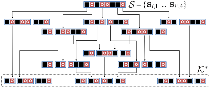
Figure 3: Partition tree for the two trajectories ${\bf S}_{i}=\{{\bf s}_{i,j}\}$ and ${\bf S}_{i^{\prime}}=\{{\bf s}_{i^{\prime},j}\}$ in Fig. 2. Nodes in the complete tree represent the set ${\cal K}$ of valid partitions of the set of raw samples ${\cal S}$. Elementary partitions are the tree leaves and constitute ${\cal K}^{*}$. The partition in Fig. 2 is the leftmost leaf in the tree.

If we build a tree of partitions belonging to ${\cal K}$, such that the ${\cal S}$ is the root and each node is a partition whose children are its refinements, the leaves are the elementary partitions, which form a subset ${\cal K}^{*}$. The above proposition states that we can limit the search of ${\bf G}^{*}$ to ${\cal K}^{*}$, drastically reducing the search space of ${\bf G}^{*}$ to the set ${\cal K}^{*}\subset{\cal K}$ of elementary partitions of ${\cal S}$. An example is provided in Fig. 3, for the trajectories in Fig. 2.

III-D Optimal merging algorithm

We propose k-merge, an algorithm to efficiently search the set of raw samples ${\cal S}$, extract the subset of elementary partitions, ${\cal K}^{*}$, and identify the optimal partition ${\bf G}^{*}$.

input : Trajectories ${\bf S}_{1},\dots,{\bf S}_{k}$, where ${\bf S}_{i}=({\bf s}_{i,1},\dots,{\bf s}_{i,N_{i}})$

output : Generalized sample set ${\bf G}^{*}$, Cost $C\left({\bf G}^{*}\right)$

1 foreach $i\in[1,k]$ do

2       ${\cal S}_{i}=\bigcup_{j=1}^{N_{i}}\{{\bf s}_{i,j}\}$;

3      

4${\cal S}$ $\leftarrow$ timesort (${\cal S}_{1}\cup\dots\cup{\cal S}_{k}$);

5 Cost $\leftarrow$ $(0,\infty,\dots,\infty)$;

6 Partition $\leftarrow$ $($NULL, $\dots$, NULL$)$;

7 foreach ${\bf s}_{\theta}\in{\cal S}$ do

8       $\theta^{\prime}=\theta-1$;

9       while incomplete (${\bf s}_{\theta^{\prime}},\ldots,{\bf s}_{\theta}$) do

10             $\theta^{\prime}=\theta^{\prime}-1$;

11            

12       while elementary (${\bf s}_{\theta^{\prime}},\ldots,{\bf s}_{\theta}$) do

13             ${\cal G}$ $\leftarrow$ generalize (${\bf s}_{\theta^{\prime}},\ldots,{\bf s}_{\theta}$);

14             if Cost $[\theta]$ $>c\left({\cal G}\right)$ + Cost $[\theta^{\prime}-1]$ then

15                   Cost $[\theta]$ $\leftarrow c\left({\cal G}\right)$ + Cost $[\theta^{\prime}-1]$;

16                   Partition $\leftarrow(\theta^{\prime}-1,{\cal G})$;

17                  

18             $\theta^{\prime}=\theta^{\prime}-1$;

19            

20      

21${\bf G}^{*}\leftarrow$ visit (Partition);

22 $C\left({\bf G}^{*}\right)\leftarrow$ Cost $[\,|{\cal S}|\,]$;

Algorithm 1 k-merge algorithm pseudocode.

The algorithm, detailed in Alg. 1, starts by populating a set of raw samples ${\cal S}$, whose items ${\bf s}_{i,j}$ are ordered according to their time value $t({\bf s}_{i,j})$ (lines 1–1). Then, it processes all samples according to their temporal ordering (line 1). Specifically, the algorithm tests, for each sample ${\bf s}_{\theta}$ in position $\theta$, all sets $\{{\bf s}_{\theta^{\prime}},\ldots,{\bf s}_{\theta}\}$, with $\theta^{\prime}<\theta$, as follows.

The first loop skips incomplete sets that do not contain at least one sample from each input trajectory (line 1). The second loop runs until the first non-elementary set is encountered (line 1). Therein, the algorithm generalizes the current (complete and elementary) set $\{{\bf s}_{\theta^{\prime}},\ldots,{\bf s}_{\theta}\}$ to ${\cal G}$, and checks if ${\cal G}$ reduces the total merging cost up to ${\bf s}_{\theta}$. If so, the cost is updated by summing $c({\cal G})$ to the accumulated cost up to ${\bf s}_{\theta^{\prime}-1}$, and the resulting (partial) partition of ${\cal S}$ that includes ${\cal G}$ is stored (lines 1–1). Once out of the loops, the cost associated to the last sample is the optimal cost, and it is sufficient to backward navigate the partition structure to retrieve the associated ${\bf G}^{*}$ (lines 1–1).

Note that, in order to update the cost of including the current sample ${\bf s}_{\theta}$ (line 1), the algorithm only checks previous samples in time. It thus needs that the optimal decision up to ${\bf s}_{\theta}$ does not depend on any of the samples in the original trajectories that come later in time than ${\bf s}_{\theta}$. The following proposition guarantees that this is the case.

Proposition 2

Let ${\bf G}^{*}=\left({\cal G}^{*}_{1},\dots,{\cal G}^{*}_{Z}\right)$ be the optimal generalized trajectory and let us make the hypothesis that ${\bf s}_{\theta}$ and ${\bf s}_{\theta+1}$ do not belong to the same generalized sample of ${\bf G}^{*}$. Let $\mathbf{G}^{*}_{\mathrm{p}}=\left({\cal G}^{*}_{1},\dots,{\cal G}^{*}_{Z_{1}}\right)$ and $\mathbf{G}^{*}_{\mathrm{f}}=\left({\cal G}^{*}_{Z_{1}+1},\dots,{\cal G}^{*}_{Z}\right)$, so that ${\bf s}_{\theta}\in{\cal G}^{*}_{Z_{1}}$ and ${\bf s}_{\theta+1}\in{\cal G}^{*}_{Z_{1}+1}$. Then, $\mathbf{G}^{*}_{\mathrm{p}}$ can be derived independently of $\mathbf{G}^{*}_{\mathrm{f}}$.

Proof: Let $\mathbf{G}$, $\mathbf{G}_{\mathrm{p}}$ and $\mathbf{G}_{\mathrm{f}}$ be any generalized sequences containing raw samples $({\bf s}_{1},\dots,{\bf s}_{N})$, $({\bf s}_{1},\dots,{\bf s}_{\theta})$ and $({\bf s}_{\theta+1},\dots,{\bf s}_{N})$, respectively. According to the cost definition, we generally have

$$\min_{\mathbf{G}}C(\mathbf{G}) \leq \min_{\mathbf{G}_{\mathrm{p}},\mathbf{G}_{\mathrm{f}}}C((\mathbf{G}_{\mathrm{p}},\mathbf{G}_{\mathrm{f}}))$$

$$= \min_{\mathbf{G}_{\mathrm{p}}}C(\mathbf{G}_{\mathrm{p}})+\min_{\mathbf{G}_{\mathrm{f}}}C(\mathbf{G}_{\mathrm{f}}),$$

where $(\mathbf{G}_{\mathrm{p}},\mathbf{G}_{\mathrm{f}})$ is the concatenation of $\mathbf{G}_{\mathrm{p}}$ and $\mathbf{G}_{\mathrm{f}}$. However, by virtue of the hypothesis and by construction,

$$\min_{\mathbf{G}}C(\mathbf{G}) = C({\bf G}^{*})$$

$$= C(\mathbf{G}^{*}_{\mathrm{p}})+C(\mathbf{G}^{*}_{\mathrm{f}})$$

$$= \min_{\mathbf{G}_{\mathrm{p}}}C(\mathbf{G}_{\mathrm{p}})+\min_{\mathbf{G}_{\mathrm{f}}}C(\mathbf{G}_{\mathrm{f}})$$

so that, to minimize $C(\mathbf{G})$ we only need to minimize $C(\mathbf{G}_{\mathrm{p}})$ and $C(\mathbf{G}_{\mathrm{f}})$ independently.  

The above proposition guarantees that the algorithm is exploring all possibilities, and as a result, the cost $C({\bf G}^{*})$ returned by k-merge is optimal, i.e., it is the minimum loss of granularity necessary to merge the original trajectories.

Note that k-merge has a very low complexity in practical cases. Let $l(\theta)$ be the number of sets $\{{\bf s}_{\theta^{\prime}},\ldots,{\bf s}_{\theta}\}$ that are both complete and elementary for a given $\theta$. Then, the number of computations and comparisons of sample generalization costs that are performed in k-merge is $\sum_{\theta}l(\theta)=|{\cal S}|\overline{l}$, where $\overline{l}$ is the average value of $l(\theta)$. If $\overline{l}=\mathcal{O}(1)$, which happens in most trajectory data where the samples of the input trajectories are intercalated in the time axis, then k-merge runs in a time $\mathcal{O}(|{\cal S}|)$, i.e., linear in the number of samples.

III-E Single user $k^{\tau,\epsilon}$-anonymity

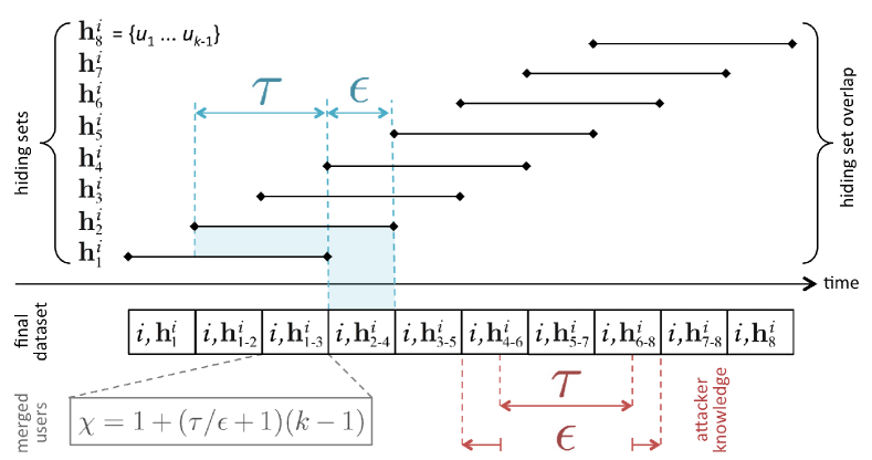
Figure 4: Overlapping hiding set structure realizing $k^{\tau,\epsilon}$-anonymity for user $i$.

We implement $k^{\tau,\epsilon}$-anonymity for a generic subscriber $i$ as shown in Fig. 4. We discretize time into intervals of length $\epsilon$, named epochs. At the beginning of the $m$-th epoch, we select a set of $k-1$ users different from $i$, named a hiding set of $i$ and denoted as ${\bf h}^{i}_{m}$. The hiding set ${\bf h}^{i}_{m}$ provides $k$-anonymity to subscriber $i$ for a subsequent time window $\tau+\epsilon$. By repeating the hiding set selection for all epochs, $\tau/\epsilon+1$ subsequent hiding sets of user $i$ overlap at any point in time. Such a structure of overlapping hiding sets assures the following.

First, subscriber $i$ is $k$-anonymized for any possible knowledge of the attacker. No matter where a time interval of length $\tau$ is shifted to along the time dimension, it will be always completely covered by the time window of one hiding set, i.e., a period during which $i$’s trajectory is indistinguishable from those of $k-1$ other users. As an example, in Fig. 4, the attacker knowledge $\tau$ (bottom-right of the plot) is fully enclosed in the time window of ${\bf h}^{i}_{6}$, and his sub-trajectory is indistinguishable from those of users in ${\bf h}^{i}_{6}$.

Second, the additional knowledge leaked to the attacker is exactly $\epsilon$. From the first point above, the adversary cannot tell apart $i$ from the users in the hiding set ${\bf h}^{i}_{m}$ whose time window covers his knowledge $\tau$. However, the adversary can follow the (generalized) trajectories of $i$ and users in ${\bf h}^{i}_{m}$ for the full time window $\tau+\epsilon$. Therefore, the adversary can infer new information about the (generalized) trajectory of $i$ during the time window period that exceeds his original knowledge $\tau$, i.e., $\epsilon$. E.g., in Fig. 4, the time window of ${\bf h}^{i}_{6}$ spans before and after the attacker knowledge $\tau$, for a total of $\epsilon$.

The two guarantees above let $k^{\tau,\epsilon}$-anonymity, as defined in Sec. II-C2, be fulfilled for the generic user $i$. The epoch duration $\epsilon$ maps to the knowledge leakage. The following important remarks are in order.

1. Hiding set selection. The structure of overlapping hiding sets is to be implemented so that the loss of accuracy in the $k^{\tau,\epsilon}$-anonymized trajectory is minimized. Thus, the users in the generic hiding set ${\bf h}^{i}_{m}$ shall be those who, during the time window $\tau+\epsilon$ starting at the $m$-th epoch, have sub-trajectories with minimum k-merge cost with respect to $i$’s.

2. Reuse constraint. The uninformative principle requires alternating the $k-1$ trajectories used in different hiding sets, as per Sec. II-C2. A simple way to enforce this is limiting the inclusion of any subscriber in at most one hiding set of $i$.

3. Generalization set. As evidenced by the example in Fig. 4, the configuration of hiding sets changes at every epoch, and $\tau/\epsilon+1$ hiding sets overlap during each epoch. This means that a spatiotemporal generalization must be used to merge a set of $\chi=1+(\tau/\epsilon+1)(k-1)$ trajectories at each epoch.

4. Epoch duration tradeoff. The epoch duration $\epsilon$ is a configurable system parameter, whose setting gives rise to a tradeoff between knowledge leakage and accuracy of the anonymized data. A lower $\epsilon$ reduces knowledge leakage. However, it also increases $\chi$, which typically entails a more marked generalization and a higher loss of data granularity.

III-F Multiple user $k^{\tau,\epsilon}$-anonymity

Scaling $k^{\tau,\epsilon}$-anonymity from a single user to all subscribers in a dataset implies that the choice of hiding sets cannot be made independently for every user. Therefore, trajectory similarity and reuse constraint fulfillment are not sufficient norms anymore. In addition to the above, the selection of hiding sets needs to be concerted among all users so as to ensure that the generalized trajectories are correctly intertwined and all subscribers are $k$-anonymized during each time window $\tau+\epsilon$.

An intuitive solution is enforcing full consistency: including a subscriber $i$ into the hiding set of user $i^{\prime}$ at epoch $m$ makes $i^{\prime}$ automatically become part of $i$’s hiding set at the same epoch. Formally, $i\in{\bf h}^{i^{\prime}}_{m}\Rightarrow i^{\prime}\in{\bf h}^{i}_{m}$, $\forall i\neq i^{\prime},\forall m$.

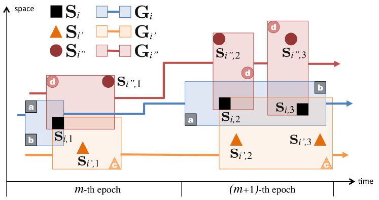
Figure 5: Example of $k$-pick constraint, with $k$=3, for user $i$ during the $m$-th hiding set selection. Here $\epsilon=\tau$, hence the time windows of hiding sets span two epochs. For clarity, space is unidimensional. Figure best viewed in colors.

In fact, full consistency is an unnecessarily restrictive condition. It is sufficient that hiding set concertation satisfies a $k$-pick constraint: during the $m$-th epoch, each user $i$ in the dataset has to be picked in the hiding sets of at least other $k-1$ subscribers. Formally, $|\{i^{\prime},\;i\in{\bf h}^{i^{\prime}}_{m}\}|\geq k-1$, $\forall i,\forall m$. This provides an increased flexibility over all existing approaches which rely on fully consistent generalization strategies.

The rationale behind the $k$-pick constraint is best illustrated by means of a toy example, in Fig. 5. The figure portrays the spatiotemporal samples of users $i$, $i^{\prime}$ and $i^{\prime\prime}$ during epochs $m$ and $m+1$. The sub-trajectory of subscriber $i$ in this time interval is ${\bf S}_{i}=({\bf s}_{i,1},{\bf s}_{i,2},{\bf s}_{i,3})$, represented as black squares; equivalently for $i^{\prime}$ (orange triangles) and $i^{\prime\prime}$ (red circles). Samples denoted by letters belong to other users $a$, $b$, $c$ and $d$, and they are instrumental to our example.

Let us assume that $\epsilon=\tau$ (i.e., hiding sets span an interval $2\tau=2\epsilon$, or epochs $m$ and $m+1$), and $k=3$. At the beginning of the $m$-th epoch, for subscriber $i$ (resp., $i^{\prime}$ and $i^{\prime\prime}$), one needs to select $k-1=2$ other users that constitute the hiding set ${\bf h}^{i}_{m}$ (resp., ${\bf h}^{i^{\prime}}_{m}$ and ${\bf h}^{i^{\prime\prime}}_{m}$). Let us consider ${\bf h}^{i}_{m}$=$\{a,b\}$, ${\bf h}^{i^{\prime}}_{m}$=$\{i,c\}$, ${\bf h}^{i^{\prime\prime}}_{m}$=$\{i,d\}$, which results in the generalized sub-trajectories ${\cal G}_{i}$, ${\cal G}_{i^{\prime}}$, ${\cal G}_{i^{\prime\prime}}$ in Fig. 5. The configuration satisfies the $k$-pick constraint for subscriber $i$, who is picked in $k-1=2$ hiding sets, i.e., ${\bf h}^{i^{\prime}}_{m}$ and ${\bf h}^{i^{\prime\prime}}_{m}$. Suppose now that the attacker knows the spatiotemporal samples of $i$’s trajectory during any time interval $\tau$ within the $m$-th and $(m+1)$-th epoch: as these samples are within ${\cal G}_{i}$, ${\cal G}_{i^{\prime}}$ and ${\cal G}_{i^{\prime\prime}}$, then $i$ is $3$-anonymized.

The key consideration is that $i$ is $k$-anonymized at epoch $m$ by $i^{\prime}$ and $i^{\prime\prime}$, yet it does not contribute to the anonymization of neither $i^{\prime}$ nor $i^{\prime\prime}$, as $i^{\prime},i^{\prime\prime}\notin{\bf h}^{i}_{m}$. Thus, it is possible to decouple the choice of hiding sets across subscribers, without jeopardizing the privacy guarantees granted by $k$-anonymity. Such a decoupling entails a dramatic increase of flexibility in the choice of hiding sets, as per the following proposition.

Proposition 3

Given a dataset of $U$ trajectories and a fixed value of $k$, the number of hiding set configurations allowed by full consistency is a fraction of that allowed by $k$-pick that vanishes more than exponentially for $U\to\infty$.

Proof: Let us consider a set of $U$ users, where $U$ is a multiple of $k$, since otherwise full consistency cannot even be enforced. Let us build a $k\times U$ matrix, in which the $i$-th column contains $(i,{\bf h}^{i}_{m})$, where ${\bf h}^{i}_{m}$ is the hiding set for user $i$ at a given epoch $m$. (For simplicity, in this proof, we do not take into account the reuse constraints.)

The solution set under the $k$-pick constraint coincides with the set of normalized Latin rectangles of size $k\times U$. Let $K_{k,U}$ be the number of $k\times U$ normalized Latin rectangles, which equals the number of possible solutions for our problem with the $k$-pick constraint. An old result by Erdős and Kaplansky [20] states that, for $U\to\infty$ and $k=O\left((\log U)^{3/2-\epsilon})\right)$,

$$K_{k,U}\sim(U!)^{k-1}\exp\left(-k(k-1)/2\right)$$ (12)

If, instead, we enforce full consistency, then the number of solutions equals the number of different partitions of a size-$U$ set into $U/k$ subsets, all with size $k$. Denoting by $C_{k,U}$ this number, we can compute it as

$$C_{k,U}=\frac{{U\choose k}{U-k\choose k}\cdot\dots\cdot{k\choose k}}{\left(U/k\right)!}=\frac{U!}{(k!)^{U/k}\left(U/k\right)!}$$ (13)

Thus, for fixed $k$ and $U\to\infty$

$$\frac{C_{k,U}}{K_{k,U}}\sim\frac{\exp\left(k(k-1)/2\right)}{(U!)^{k-2}(k!)^{U/k}\left(U/k\right)!}$$

which tends to zero more than exponentially for $U\to\infty$.  

For large datasets of hundreds of thousands trajectories, $k$-pick enables a much richer choice of merging configurations. This reasonably unbinds better combinations of the original trajectories, and results in more accurate anonymized data.

III-G Practical $k^{\tau,\epsilon}$-anonymity algorithm

Capitalizing on all previous results, we design kte-hide, an algorithm that achieves $k^{\tau,\epsilon}$-anonymity in datasets of spatiotemporal trajectories. Since even the optimal solution to the simpler $k$-anonymity problem is known to be NP-hard [14], we resort here to an heuristic solution.

input : Anonymization level $k$, attacker knowledge $\tau$, leakage $\epsilon$

input : Trajectory dataset $\mathbb{D}$

output : Anonymized trajectory dataset $\mathbb{D}$

1 foreach $e_{\theta}\in$ epochs ($\mathbb{D}$) do

2       $\mathbb{D}_{f}$ $\leftarrow$ filter ($e_{\theta},\mathbb{D}$);

3       foreach ${\bf S}_{i},{\bf S}_{i^{\prime}}\in\mathbb{D}_{f},{\bf S}_{i}\neq{\bf S}_{i^{\prime}}$ do

4             Costs [${\bf S}_{i},{\bf S}_{i^{\prime}}$] $\leftarrow$ k-merge (${\bf S}_{i},{\bf S}_{i^{\prime}}$);

5            

6       Clusters [$\theta$] $\leftarrow$ spectralClustering (Costs);

7       if $\theta\geq\tau/\epsilon+1$ then

8             foreach $\texttt{c}\in$ Clusters [$\theta$] do

9                   Subs $\leftarrow$ split (c,Clusters [$\theta-\tau/\epsilon$ : $\theta-1$]);

10                   foreach $\texttt{c}_{s}\in$ Subs [$\theta$] do

11                         $\texttt{g}_{s}\leftarrow$ graph ($\texttt{c}_{s}$);

12                         $\texttt{g}_{sc}\leftarrow$ greedyCycle ($\texttt{g}_{s}$,$k$);

13                         if $\exists\texttt{g}_{sc}$ then

14                               foreach ${\bf S}_{i}\in\texttt{c}_{s}$ do

15                                     ${\bf h}^{i}_{\theta-\tau/\epsilon}\leftarrow\texttt{g}_{sc}$[${\bf S}_{i}$];

16                                    

17                              

18                        else

19                               suppression ($\texttt{c}_{s}$);

20                              

21foreach $e_{\theta}\in$ epochs ($\mathbb{D}$) do

22       foreach ${\bf S}_{i}\in\mathbb{D}$ do

23             ${\bf h}\leftarrow$ filter ($e_{\theta},{\bf S}_{i},{\bf h}^{i}_{\theta-\tau/\epsilon},\dots,{\bf h}^{i}_{\theta}$);

24             $\mathbb{D}\leftarrow$ replace (k-merge (${\bf h}$));

25            

Algorithm 2 kte-hide algorithm pseudocode.

The algorithm, in Alg. 2, proceeds on a per-epoch basis (line 2), finding, for each epoch $\theta$, a set of $\chi$ users (with $\chi$ defined as in Sec. III-E) that hide each subscriber at low merging cost. An extensive search for the set of $\chi$ users would have an excessive cost ${\cal O}(U^{\chi})$, where $U$ is the number of users in dataset, and $\chi\geq 3$. Thus, we adopt a computationally efficient approach, by clustering user sub-trajectories based on their pairwise merging cost. Costs are computed via k-merge (lines 2–2), and a standard spectral clustering algorithm groups similar trajectories into same clusters (line 2). This allows operating on each cluster independently in the following.

Starting from epoch $\tau/\epsilon+1$ (line 2), the algorithm processes each identified cluster at epoch $\theta$ separately (line 2). It splits the current cluster $c$ into subsets, which contain user trajectories that share the same sequence of clusters during the last $\tau/\epsilon$ epochs (line 2).

Let $c_{s}$ be any of such subsets: $c_{s}$ is mapped to a directed graph whose nodes are the users within $c_{s}$, and there is an edge going from user $j$ to user $i$ if $j$ can be in the hiding set ${\bf h}^{i}_{\theta-\tau/\epsilon}$ of $i$ without violating the reuse constraint (line 2). If a $k$-anonymity level is required, $k-1$ directional cycles are then built within the graph, involving all nodes in the graph, in such a way that each node has a different parent in each cycle (line 2). The hiding set ${\bf h}^{i}_{t-\tau/\epsilon}$ is then obtained as the set of user $i$’s parents in the $k-1$ cycles (lines 2–2).

Such a construction of hiding sets complies with the $k$-pick constraint, since every user $i$ is in the hiding set of $k-1$ other users. It may however happen that no valid $k-1$ cycles can be created within $c_{s}$: this means that subscribers in $c_{s}$ share a sub-trajectory that is rare in the dataset, and their number is insufficient to implement $k^{\tau,\epsilon}$-anonymity. In this case, we apply suppression and remove all spatiotemporal samples of such users’ sub-trajectories (line 2). Once all hiding sets are determined, the merging is performed, on each epoch and for each user, using k-merge (lines 2–2).

Overall, the heuristic algorithm above guarantees that overlapping hiding sets that satisfy the reuse constraint (Sec. III-E) are selected for all users. It also ensures that such a choice of hiding sets fulfils the $k$-pick requirement (Sec. III-F). Together, these conditions realize $k^{\tau,\epsilon}$-anonymity of the trajectory data.

The complexity of kte-hide is as follows. Let $U$ be the number of users, $\Theta$ be the number of epochs and $\overline{{\cal N}}$ be the average number of samples per user per epoch, so that ${\cal N}_{tot}=\Theta U\overline{{\cal N}}$ is the total number of samples in the dataset. Then: (i) lines 2–2 perform k-merge on two input trajectories $\Theta U^{2}$ times, each of them with a complexity ${\cal O}(\overline{{\cal N}})$, for a total complexity of ${\cal O}({\cal N}_{tot}U)$; (ii) spectral clustering (line 2) can be implemented with complexity ${\cal O}(\Theta U^{2})$ using KASP [21]; (iii) the complexity of lines 2–2, performing k-merge on $\chi$ input trajectories $\Theta U$ times, is ${\cal O}({\cal N}_{tot}\chi)$. All other subroutines of kte-hide have a much smaller complexity.

TABLE I: Features of reference mobile traffic datasets.

Dataset	Surface	BS	BS/Km2	Users	Density	Samples	Timespan
	[Km2]				[user/Km2]	[per user/h]	[days]
abi	2,731	400	0.14	29,191	10.68	0.90	14
dak	1,024	457	0.44	71,146	69,47	0.74	14
shn	3,329	2961	0.89	50,000	15.01	1.00	1
civ	322,463	1238	0.0038	82,728	0.26	0.75	14
sen	196,712	1666	0.0085	286,926	1.45	0.45	14

TABLE II: Comparative performance evaluation of k-merge

Dataset	$k$	k-merge		Static generalization [success %]			W4M				GLOVE
		Time	Space	2h - 4Km	4h - 10Km	8h - 20Km	Deleted	Created	Time	Space	Time	Space
		[min]	[Km]				[%]	[%]	[min]	[Km]	[min]	[Km]
abi	2	51	0.624	27.2	56.7	80.3	9.6	22.0	57	1.166	114	2.626
	5	228	3.423	0.7	11.0	40.5	31.9	31.2	185	3.809	292	3.740
	8	349	5.720	0.1	5.1	22.6	23.9	36.7	198	6.163	—	—
dak	2	47	0.701	43.2	68.7	93.3	5.9	11.4	39	1.466	116	2.498
	5	220	5.286	2.2	14.0	67.0	20.3	21.2	172	5.807	294	3.192
	8	377	7.794	0.1	8.6	50.7	22.0	18.6	189	8.477	—	—

IV Performance evaluation

We evaluate our anonymization solutions with five real-world datasets of mobile subscriber trajectories, introduced in Sec. IV-A. A comparative evaluation of k-merge is in Sec. IV-B, while the results of $k^{\tau,\epsilon}$-anonymization via kte-hide are presented in Sec. IV-C.

IV-A Reference datasets

Our datasets consist of user trajectories extracted from call detail records (CDR) released by Orange within their D4D Challenges [22], and by the University of Minnesota [23]. Three datasets, denoted as abi, dak and shn, describe the spatiotemporal trajectories of tens of thousands mobile subscribers in urban regions, while the other two, civ and sen hereinafter, are nationwide. In all datasets, user positions map to the latitude and longitude of the current base station (BS) they are associated to. The main features of the datasets are listed in Tab. II, revealing the heterogeneity of the scenarios.

In order to ensure that all datasets yield a minimum level of detail in the trajectory of each tracked subscriber, we had to preprocess the abi and civ datasets. Specifically, we only retained those users whose trajectories have at least one spatiotemporal sample on every day in a specific two-week period. No filtering was needed for the dak and sen datasets, which already contain users who are active for more than 75% of a 2-week timespan, and shn, whose users have even higher sampling rates.

In all datasets, user positions map to the latitude and longitude of the current base station (BS) they are associated to. We discretized the resulting positions on a 100-m regular grid, which represents the finest spatial granularity we consider.

Samples are timestamped with an precision of one minute. This is the granularity granted in the abi and civ datasets. The dak and sen datasets feature a temporal granularity of 10 minutes: in order to have comparable datasets, we added a random uniform noise over a ten-minute timespan to each sample, so as to artificially refine the time granularity of the data to one minute as well. In the case of the shn dataset, the precision is one second, and we used a one-minute binning to uniform the data to the standard format.

IV-B Comparative evaluation of k-merge

Since no previous solution for $k^{\tau,\epsilon}$-anonymity exists, we are forced to compare our algorithms to previous techniques in terms of simpler $k$-anonymity. Interestingly, this allows validating our proposed approach for merging spatiotemporal trajectories via the k-merge algorithm.

We thus run k-merge on 100 random $k$-tuples of mobile users from the reference datasets, for different values of $k$, and we record the spatiotemporal granularity retained by the resulting generalized trajectories. We compare our results against those obtained by the only three approaches proposed in the literature for the $k$-anonymization of trajectories along both spatial and temporal dimensions.

The first is static generalization [8, 9], which consists in a homogeneous reduction of data granularity, decided arbitrarily and imposed on all user trajectories. Static generalization is a trial-and-error process, and it does not guarantee $k$-anonymity of all users. The second benchmark solution is Wait for Me (W4M) [36]. Intended for regularly sampled (e.g., GPS) trajectories, W4M performs the minimum spatiotemporal translation needed to push all the trajectories within the same cylindrical volume. It allows the creation of new synthetic samples, and it is thus not fully compliant with PPDP principles in Sec. II-A. The latter operation is leveraged to improve the matching among trajectories in a cluster, and assumes that mobile objects (i.e., subscribers in our case) effectuate linear constant-speed movements between spatiotemporal samples. We use W4M with linear spatiotemporal distance (W4M-L), i.e., the version intended for large databases such as those we consider , and configure it with the settings suggested in [36]. The third approach is GLOVE [10], which relies on a heuristic measure of anonymizability to assess the similarity of spatiotemporal trajectories. This measure is fed to a greedy algorithm to achieve $k$-anonymity with limited loss of granularity and without introducing fictitious data. However, unlike k-merge, GLOVE does not provide an optimal solution, and is computationally expensive.

The results of our comparative evaluation are summarized in Tab. II, for the abi and dak datasets, when varying number $k$ of trajectories merged together. Similar results were obtained for the other datasets, and are omitted due to space limitations. We immediately note how static aggregation is an ineffective approach: the percentage of successfully merged $k$-tuples is well below 100%, even when dramatically reducing the data granularity to 8 hours in time and 20 km in space. Instead, k-merge, W4M and GLOVE can merge all of the $k$-tuples, while retaining a good level of accuracy in the data. We can directly compare the granularity in time (min) and space (km) retained by k-merge, W4M and GLOVE in merging groups of $k$ trajectories: the spatiotemporal accuracy is comparable in all cases. However, it is important to note that W4M attains this result by deleting and creating a significant amount of samples: in the end, only 40-70% of the original samples are maintained in the generalized data. Conversely, all of the generalized samples created by k-merge reflect the actual real-world data. Also, k-merge obtains a level of precision that is always higher than that of GLOVE, and scales better: indeed, the complexity of GLOVE did not allow computing a solution when $k=8$.

Overall, the results uphold k-merge as the current state-of-the-art solution to generalize sparse spatiotemporal trajectories while obeying PPDP principles and minimizing accuracy loss.

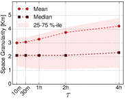
(a) abi

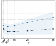
(b) dak

(c) shn

(d) abi

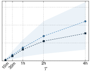
(e) dak

(f) shn

Figure 6: Spatial (a,b,c) and temporal (d,e,f) granularity versus the adversary knowledge $\tau$ in the citywide reference datasets.

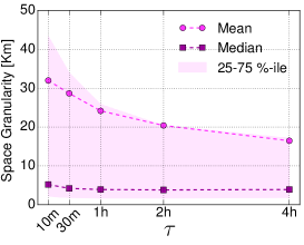
(a) civ

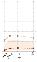
(b) sen

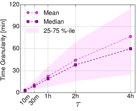
(c) civ

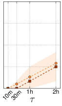
(d) sen

Figure 7: Spatial (a,b) and temporal (c,d) granularity versus $\tau$ in the nationwide reference datasets.

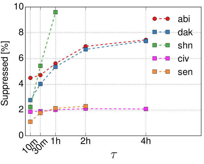
Figure 8: Suppressed samples versus $\tau$.

IV-C Performance evaluation of kte-hide

We run kte-hide on our reference datasets of mobile subscriber trajectories, so that they are $k^{\tau,\epsilon}$-anonymized. As the anonymized data are robust to probabilistic attacks by design, we focus our evaluation on the cost of the anonymization, i.e., the loss of granularity. All results refer to the case of $2^{\tau,\epsilon}$-anonymization, with $\epsilon=\tau$.

IV-C1 Citywide datasets

Fig. 6 portrays the mean, median and first/third quartiles of the sample granularity in the $k^{\tau,\epsilon}$-anonymized citywide datasets abi, dak and shn. The plots show how results vary when the adversary knowledge $\tau$ ranges from 10 minutes to 4 hours. They refer to the anonymized data granularity in space, in Fig.6a-LABEL:sub@fig:pos_gran_vs_t_shn and time, in Fig.6d-LABEL:sub@fig:tim_gran_vs_t_shn.

We remark how the $k^{\tau,\epsilon}$-anonymized datasets retain significant levels of accuracy, with a median granularity in the order of 1-3 km in space and below 45 minutes in time. These levels of precision are largely sufficient for most analyses on mobile subscriber activities, as discussed in, e.g., [24]. The temporal granularity is negatively affected by an increasing adversary knowledge $\tau$, which is expected. Interestingly, however, the spatial granularity is only marginally impacted by $\tau$: protecting the data from a more knowledgeable attacker does not have a significant cost in terms of spatial accuracy.

IV-C2 Nationwide datasets

Fig. 8 shows equivalent results for the nationwide datasets civ and sen. The evolution of temporal granularity versus $\tau$, in Fig.7c-LABEL:sub@fig:tim_gran_vs_t_sen is consistent with citywide scenarios. Differences emerge in terms of spatial granularity: in the civ case (Fig.7a) a reversed trend emerges, as accuracy grows along with the attacker knowledge. This counterintuitive result is explained by the thin user presence in the civ dataset: as per Tab. II, civ has a density of subscribers per Km² that is one or two orders of magnitude lower than those in our other reference datasets. Such a geographical sparsity makes it difficult to find individuals with similar spatial trajectories: increasing $\tau$ has then the effect of enlarging the set of candidate trajectories for merging at each epoch, with a positive influence on the accuracy in the generalized data.

These considerations are confirmed by the results with the sen dataset (Fig.7b). As per Tab. II, this dataset features a subscriber density that is about one order of magnitude higher than that of civ, but around one order of magnitude lower than those of the abi, dak and shn. Coherently, the spatial granularity trend falls in between those observed for such datasets, and it is not positively or negatively impacted by the attacker knowledge.

More generally, the results in Fig. 8 demonstrate that kte-hide can scale to large-scale real-world datasets. The absolute performance is good, as the $k^{\tau,\epsilon}$-anonymized data retains substantial precision: the median levels of granularity in space and time are comparable to those achieved in citywide datasets. Finally, we remark that, in all cases, the amount of samples suppressed by kte-hide is in the 1%–7% range.

IV-C3 Sample suppression

The amount of samples suppressed by kte-hide in the $k^{\tau,\epsilon}$-anonymization process is portrayed in Fig. 8. We note that resorting to suppression becomes more frequent as the adversary knowledge increases. However, even when the opponent is capable of tracking a user during four continued hours, the percentage of suppressed samples remains low, typically well below 10%. Moreover, the trend in the long-timespan datasets is clearly sublinear, suggesting that suppression does not become prevalent with higher $\tau$. Results are fairly consistent across citywide datasets. Nationwide datasets are also aligned, and yield even lower suppression rates, at around 2%. This difference is explained by the fact that a larger number of users allows for a more efficient spectral clustering in kte-hide.

IV-C4 Disaggregation over time

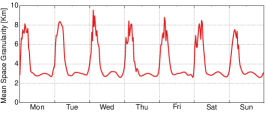
(a) abi, space

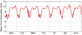
(b) abi, time

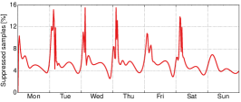
(c) abi, suppression

Figure 9: Time series of spatiotemporal accuracy (a,b) and suppression usage (c) for one sample week in the abi dataset.

As an intriguing concluding remark, Fig. 9 reveals a clear circadian rhythm in the granularity of $k^{\tau,\epsilon}$-anonymized data, as well as in the percentage of suppressed samples. The plots refer to one sample week in the abi and dak datasets, when $\tau$ = 30 min, but consistent results were observed in all of our reference datasets. Specifically, the mean spatial granularity, in Fig. 9a, is much finer during daytime, when subscribers are more active and the volume of trajectories is larger: here, it is easier to hide a user into the crowd. Overnight displacements are instead harder to anonymize, since subscribers are limited in number and they tend to have diverse patterns. This is also corroborated by the significantly higher suppression of samples between midnight and early morning, in Fig. 9c. Time granularity, in Fig. 9b, is less subject to day-night oscillations: the slightly higher accuracy recorded at night is an artifact of the important relative suppression of samples at those times.

IV-C5 Summary

Overall, our results show that kte-hide attains $k^{\tau,\epsilon}$-anonymity of real-world datasets of mobile traffic, while maintaining a remarkable level of accuracy in the data. Interestingly, its performance is better when most needed, at daytime, when the majority of human activities take place.

V Related work

Protection of individual mobility data has attracted significant attention in the past decade. However, attack models and privacy criteria are very specific to the different data collection contexts. Hence, solutions developed for a specific type of movement data are typically not reusable in other environments.

For instance, a vast amount of works have targeted user privacy in location-based services (LBS). There, the goal is ensuring that single georeferenced queries are not uniquely identifiable [25]. This is equivalent to anonymizing each spatiotemporal sample independently, and a whole other problem from protecting full trajectories. Even when considering sequences of queries, the LBS milieu allows pseudo-identifier replacement, and most solutions rely on this approach, see, e.g., [26, 27]. If applied to spatiotemporal trajectories, these techniques would seriously and irreversibly break up trajectories in time, disrupting data utility.

Another popular context is that of spatial trajectories that do not have a temporal dimension. The problem of anonymizing datasets of spatial trajectories has been thoroughly explored in data mining, and many practical solutions based on generalization have been proposed, see, e.g., [29, 28, 30, 31]. Such solutions are not compatible with or easily extended to the more complex spatiotemporal data we consider.

Some works explicitly target privacy preservation of spatiotemporal trajectories. However, the precise context they refer to makes again all the difference. First, most such solutions consider scenarios where user movements are sampled at regular time intervals that are identical for all individuals [33, 32], or where the number of samples per device is very small [34]. These assumptions hold, e.g., for GPS logs or RFID record, but not for trajectories recorded by mobile operators: the latter are irregularly sampled, temporally sparse, and cover long time periods, which results in at least hundreds of samples per user. Second, many of the approaches above disrupt data utility, by, e.g., trimming trajectories [35], or violate the principles of PPDP, by, e.g., perturbating or permutating the trajectories [33, 32], or creating fictitious samples [36]. Third, all previous studies aim at attaining $k$-anonymity of spatiotemporal trajectories, i.e., they protect the data against record linkage; this includes recent work specifically tailored to mobile subscriber trajectory datasets [10]. As explained in Sec. II, $k$-anonymity is only a partial countermeasure to attacks on spatiotemporal trajectories.

Provable privacy guarantees are instead offered by differential privacy, which commends that the presence of a user’s data in the published dataset should not change substantially the output of the analysis, and thus formally bounds the privacy risk of that user [37]. There have been attempts at using differential privacy with mobility data. Specifically, it has been successfully used the in the LBS context, when publishing aggregate information about the location of a large number of users, see, e.g., [38]. However, the requirements of these solutions already become too strong in the case of individual LBS access data [39]. To address this problem, a variant of differential privacy, named geo-indistinguishability has been introduced: it requires that any two locations become more indistinguishable as they are geographically closer [40]. Practical mechanisms achieve geo-indistinguishability, see, e.g., [39, 40]. However, all refer to the anonymization of single LBS queries: as of today, differential privacy and its derived definitions still appear impractical in the context of spatiotemporal trajectories.

VI Conclusions

In this paper, we presented a first PPDP solution to probabilistic and record linkage attacks against mobile subscriber trajectory data. To that end, we introduced a novel privacy model, $k^{\tau,\epsilon}$-anonymity, which generalizes the popular criterion of $k$-anonymity. Our proposed algorithm, kte-hide, implements $k^{\tau,\epsilon}$-anonymity in real-world datasets, while retaining substantial spatiotemporal accuracy in the anoymized data.

References

- [1] K. Zheng, Z. Yang, K. Zhang, P. Chatzimisios, K. Yang, W. Xiang, “Big data-driven optimization for mobile networks toward 5G,” IEEE Network, 30(1), 2016.
- [2] M. Leconte, G. Paschos, L. Gkatzikis, M. Draief, S. Vassilaras, S. Chouvardas, “Placing Dynamic Content in Caches with Small Population,” IEEE INFOCOM, 2016.
- [3] Telefonica Smart Steps, http://dynamicinsights.telefonica.com/smart-steps/.
- [4] Orange Flux Vision, http://www.orange-business.com/fr/produits/flux-vision.
- [5] D. Naboulsi, M. Fiore, R. Stanica, S. Ribot, “Large-scale Mobile Traffic Analysis: a Survey,” IEEE Communications Surveys and Tutorials, 18(1), 2016.
- [6] M. T. Asif, N. Mitrovic, J. Dauwels, P. Jaillet, “Matrix and Tensor Based Methods for Missing Data Estimation in Large Traffic Networks,” IEEE Transactions on ITS, 17(7), 2016.
- [7] G. Czibula, A. M. Guran, I. G. Czibula, G. S. Cojocar, “IPA - An intelligent personal assistant agent for task performance support,” IEEE ICCP, 2009.
- [8] H. Zang, J. Bolot, “Anonymization of location data does not work: A large-scale measurement study,” ACM MobiCom, 2011.
- [9] Y. de Montjoye, C.A. Hidalgo, M. Verleysen, V. Blondel, “Unique in the Crowd: The privacy bounds of human mobility,” Nature Scientific Reports, 3(1376), 2013.
- [10] M. Gramaglia, M. Fiore, “Hiding Mobile Traffic Fingerprints with GLOVE,” ACM CoNEXT, 2015.
- [11] A. Cecaj, M. Mamei, N. Bicocchi, “Re-identification of Anonymized CDR datasets Using Social Network Data,” IEEE PerCom Workshops, 2014.
- [12] C. Riederer, Y. Kim, A. Chaintreau, N. Korula, S. Lattanzi, “Linking Users Across Domains with Location Data: Theory and Validation,” ACM WWW, 2016.
- [13] J. Mayer, P. Mutchler, J.C. Mitchell, “Evaluating the privacy properties of telephone metadata,” PNAS, 113(20), 2016.
- [14] B.C.M. Fung, K. Wang, R. Chen, P.S. Yu, “Privacy-preserving data publishing: A survey of recent developments,” ACM Computing Surveys, 42(4), 2010.
- [15] L. Sweeney, “k-anonymity: A model for protecting privacy,” International Journal of Uncertainty, Fuzziness and Knowledge-Based Systems, 10(5), 2002.
- [16] A. Machanavajjhala, D. Kifer, J. Gehrke, M. Venkitasubramaniam, “l-diversity: Privacy beyond k-anonymity,” ACM Transactions on Knowledge Discovery from Data, 1(1):3, 2007.
- [17] R. Shokri, G. Theodorakopoulos, J.-Y. Le Boudec, J.-P. Hubaux, “Quantifying Location Privacy,” IEEE SP, 2011.
- [18] M. Srivatsa, M. Hicks, “Deanonymizing Mobility Traces: Using Social Networks as a Side-Channel,” AMC CCS, 2012.
- [19] M. Terrovitis, N. Mamoulis, P. Kalnis, “Privacy-preserving Anonymization of Set-valued Data,” VLDB, 2008.
- [20] P. Erdős, I. Kaplansky, “The asymptotic number of Latin rectangles,” Amer. J. Math., 68:230-236, 1946.
- [21] D. Yan, L. Huang, M.I. Jordan, “Fast approximate spectral clustering,” ACM SIGKDD, 2009.
- [22] Orange D4D Challenge. http://www.d4d.orange.com/en/.
- [23] D. Zhang, J. Huang, Y. Li, F. Zhang, C. Xu, T. He, “Exploring Human Mobility with Multi-Source Data at Extremely Large Metropolitan Scales,” ACM MobiCom, 2014.
- [24] M. Coscia, S. Rinzivillo, F. Giannotti, D. Pedreschi, “Optimal Spatial Resolution for the Analysis of Human Mobility,” IEEE/ACM ASONAM, 2012.
- [25] M. Gruteser, D. Grunwald, “Anonymous Usage of Location-Based Services Through Spatial and Temporal Cloaking,” ACM MobiSys, 2003.
- [26] J. Meyerowitz, R.R. Choudhury, “Hiding stars with fireworks: location privacy through camouflage,” ACM MobiCom, 2009.
- [27] B. Hoh, M. Gruteser, H. Xiong, A. Alrabady, Preserving privacy in GPS traces via uncertainty-aware path cloaking. ACM CSS, 2007.
- [28] A. Monreale, G. Andrienko, N. Andrienko, F. Giannotti, D. Pedreschi, S. Rinzivillo, S. Wrobel “Movement Data Anonymity through Generalization,” Transactions on Data Privacy 3(2), 2010.
- [29] M.E. Nergiz, M. Atzori, Y. Saygin, B. Güç “Towards Trajectory Anonymization: a Generalization-Based Approach,” Transactions on Data Privacy 2(1), 2009.
- [30] R. Chen, B.C.M. Fung, B.C. Desai, N.M. Sossou, “Differentially private transit data publication: a case study on the Montreal transportation system,” ACM KDD, 2012.
- [31] G. Poulis, S. Skiadopoulos, G. Loukides, A. Gkoulalas-Divanis, “Apriori-based algorithms for km-anonymizing trajectory data,” Transactions on Data Privacy 7(2), 2014.
- [32] J. Domingo-Ferrer, R. Trujillo-Rasúa, “Microaggregation- and permutation-based anonymization of movement data,” Information Science, 208, 2012.
- [33] O. Abul, F. Bonchi, M. Nanni, “Never walk alone: Uncertainty for anonymity in moving objects databases,” IEEE ICDE, 2008.
- [34] B.C.M. Fung, M. Cao, B.C. Desai, H. Xu, “Privacy protection for RFID data,” ACM SAC, 2009.
- [35] Y. Song, D. Dahlmeier, S. Bressan, “Not So Unique in the Crowd: a Simple and Effective Algorithm for Anonymizing Location Data,” PIR, 2014.
- [36] O. Abul, F. Bonchi, M. Nanni, “Anonymization of moving objects databases by clustering and perturbation,” Information Systems, 35(8), 2010.
- [37] C. Dwork “Differential privacy,” ICALP, 2006.
- [38] R. Chen, G. Acs, C. Castelluccia “Differentially private sequential data publication via variable-length n-grams,” ACM CCS, 2012.
- [39] K. Chatzikokolakis, C. Palamidessi, M. Stronati, “A Predictive Differentially-Private Mechanism for Mobility Traces,” PETS, 2014.
- [40] M.E. Andrés, N.E. Bordenabe, K. Chatzikokolakis, C. Palamidessi, “Geo-indistinguishability: differential privacy for location-based systems,” ACM CCS, 2013.