Formation and relaxation of quasi-stationary states in particle systems with power law interactions

Abstract

Abstract

We explore the formation and relaxation of so-called quasi-stationary states (QSS) for particle distributions in three dimensions interacting via an attractive radial pair potential $V(r\rightarrow\infty)\sim 1/r^{\gamma}$ with $\gamma>0$, and either a soft-core or hard-core regularization at small $r$. In the first part of the paper we generalize, for any spatial dimension $d\geq 2$, Chandrasekhar’s approach for the case of gravity to obtain analytic estimates of the rate of collisional relaxation due to two body collisions. The resultant relaxation rates indicate an essential qualitative difference depending on the integrability of the pair force at large distances: for $\gamma>d-1$ the rate diverges in the large particle number $N$ (mean field) limit, unless a sufficiently large soft core is present; for $\gamma<d-1$, on the other hand, the rate vanishes in the same limit even in the absence of any regularization. In the second part of the paper we compare our analytical predictions with the results of extensive parallel numerical simulations in $d=3$ performed with an appropriate modification of the GADGET code, for a range of different exponents $\gamma$ and soft cores leading to the formation of QSS. We find, just as for the previously well studied case of gravity (which we also revisit), excellent agreement between the parametric dependence of the observed relaxation times and our analytic predictions. Further, as in the case of gravity, we find that the results indicate that, when large impact factors dominate, the appropriate cut-off is the size of the system (rather than, for example, the mean inter-particle distance). Our results provide strong evidence that the existence of QSS is robust only for long-range interactions with a large distance behavior $\gamma<d-1$; for $\gamma\geq d-1$ the existence of such states will be conditioned strongly on the short range properties of the interaction.

today

I introduction

There are many systems of particles interacting with long-range interactions in nature: self-gravitating bodies in astrophysics and cosmology Binney and Tremaine (2008), two-dimensional fluid dynamics Chavanis (2002), cold atoms Chalony et al. (2013), etc. Considering, for simplicity, $d-$dimensional particle systems which interact through an isotropic pair potential $v(r)$, long-range systems are usually defined as those for which

$$v(r\to\infty)\sim\frac{g}{r^{\gamma}},$$ (1)

where $\gamma\leq d$, and $g$ is a coupling constant. This characterization of interactions as long-range arises in equilibrium statistical mechanics Campa et al. (2009): in a system of $N$ particles in a volume $V$, the average energy of a particle is, for $\gamma>d$, independent of the size of the system in the “usual” thermodynamic limit $N\rightarrow\infty$, $V\rightarrow\infty$ at fixed density $N/V$. For $\gamma\leq d$ a different thermodynamic limit must be taken in order to recover extensivity of the thermodynamic potentials, and $N$ independent intensive properties of the system, as $N\rightarrow\infty$. More specifically, the potential energy $\Phi_{i}$ of a particle scales as $\Phi_{i}\sim gN/V^{\gamma/d}$ and $g$ and $V$ must be scaled appropriately with $N$ so that $\Phi_{i}$ is constant. This is usually called the mean-field thermodynamic limit (or the Vlasov limit when is is taken at fixed system size). Using this scaling, the total energy becomes extensive and it is possible to compute thermal equilibrium properties. For the class of systems we consider here, with attractive power law interactions at large scales in three dimensions, such a treatment has been given in Ispolatov and Cohen (2001). For $\gamma<d$ they present unusual features compared to short range systems: inhomogeneous spatial distributions, inequivalence of the statistical ensembles, negative specific heat in the microcanonical ensemble etc..

For the case of gravity it was understood decades ago, however, in the context of astrophysics (through the seminal works of Chandrasekhar, Lynden-Bell and others) that such considerations based on equilibrium statistical mechanics are only relevant physically on time scales very long compared to those on which such systems evolve dynamically (e.g. the formation and evolution of galaxies), and that the scenario of the dynamics of such systems is completely different to that of short range systems: on a timescale $\tau_{dyn}$ characteristic of the mean field dynamics (and independent of $N$ in the mean field limit described above) one observes the formation, under the effect of a mean field global interaction through so-called mean-field relaxation, of very slowly evolving macroscopic states (e.g. galaxies) which are far from thermal equilibrium. For gravity in $d=3$ dimensions, the time scale for evolution towards equilibrium was first estimated by Chandrasekhar Chandrasekhar (1942) to be $\tau_{coll}\sim(N/\ln N)\tau_{dyn}$. Thus as $N\rightarrow\infty$ in the mean field limit, the system remains trapped in such states and never evolves towards thermodynamic equilibrium. A similar phenomenology has been established in the last years in the study of various other systems with long-range interactions (see e.g. Yamaguchi et al. (2004); Joyce and Worrakitpoonpon (2010); Teles et al. (2010); Marcos (2013)): relaxation on a mean field time scale to a “quasi-stationary state” (QSS) followed by a relaxation towards thermodynamic equilibrium on a time scale which diverges with the particle number $N$. This scenario has thus been proposed as a kind of paradigm for the dynamics of this class of interactions (e.g. Campa et al. (2009); Levin et al. (2014); Chavanis (2012a)).

More formally the evolution of a system of $N$ particles interacting through the pair potential (1) can be described by the equation

$$\frac{\partial f}{\partial t}+{\bf v}({\bf r},t)\cdot\frac{\partial f}{\partial{\bf r}}+{\mathbf{F}}[f]\cdot\frac{\partial f}{\partial{\bf v}}=C_{N}\,,$$ (2)

where $f({\bf r},{\bf v},t)$ is the mean phase space density function, i.e., the density of particles at the position ${\bf r}$ with velocity ${\bf v}$ at time $t$, and $C_{N}$ is called the “collision term”. In general the latter is a functional of the $n-point$ distribution functions. The term ${\mathbf{F}}[f]$ is the mean field force which can be written in terms of the pair potential $v(r)$ as

$${\mathbf{F}}[f]=-\int f({\bf r}^{\prime},{\bf v},t)\nabla_{{\bf r}}v(|{\bf r}-{\bf r}^{\prime}|)d{\bf r}^{\prime}d{\bf v}\,.$$ (3)

A mean-field dynamical description is valid if, in the mean-field (or Vlasov) limit, we have that

$$\lim_{N\to\infty}C_{N}=0$$ (4)

in which case the dynamics is described by the Vlasov equation, known as the “collisionless Boltzmann equation” in the astrophysical literature (e.g. Binney and Tremaine (2008)). QSS are understood as stable stationary solutions of these equations, and mean-field relaxation as the evolution towards such states in the same mean-field framework (on timescales of order $\tau_{dyn}$). Correspondingly, in any finite (but large) $N$ system, the term $C_{N}$ then describes the “collisional” corrections to the mean-field dynamics.

For long-range interactions, therefore, to show that QSS should exist one should analyze these collision terms, and determine firstly that they do indeed satisfy the condition (4). Further in order to understand their evolution away from QSS at large but finite $N$, and (possibly) towards thermal equilibrium, one needs to derive a suitable kinetic theory, which should allow one to infer the scalings of the time scale (or scales) characterizing such evolution as a function of $N$. Concerning the first step rigorous results have been obtained showing that the limit does exist in the gravitational case Braun and Hepp (1977); Spohn (1991) and for any potential with $\gamma\leq 1$ Hauray and Jabin (2007) (both in $d=3$ dimensions) and provided a suitable regularization (i.e. softening) of the potential is imposed at small separations (see also Boers and Pickl (2013); Lazarovici and Pickl (2015)). However these provide only rigorous lower bounds ($\sim logN$) to the time scales on which the Vlasov dynamics is valid. They do not allow us to calculate in any practical manner the time scales for collisional relaxation, nor even to determine their parametric scalings. Many attempts have been made in this direction through the construction of explicit kinetic theories Weinberg (1993); Heyvaerts (2010); Chavanis (2012b); Fouvry et al. (2015a, b); Fouvry and Pichon (2015); Fouvry et al. (2016a, b); Benetti and Marcos (2016) but, in practice it is difficult to apply these methods to realistic systems to establish the relevant time scales, and in particular their parametric scalings. Moreover, these theories do not take into account strong collisions. Often (e.g. Chavanis (2012a)) it is argued, using such approaches, that the characteristic time scale for collisional relaxation has a generic scaling $\tau_{\rm coll}\sim N\tau_{dyn}$, except for the special case of homogeneous QSS in one dimension.

In this paper we explore the conditions under which the limit (4) is satisfied for the generic power law interaction (1). To do so we use a non-rigorous (but well defined) approach to the problem: we generalize the simple method initiated by Chandrasekhar for the case of gravity Chandrasekhar (1942); Binney and Tremaine (2008). This amounts to assuming that the dominant contribution to the collisionality, described by the term $C_{N}$, comes from two body collisions. For the gravitational interaction this simple approach has turned out to account remarkably well for the observed time scales of collisional relaxation (in numerical simulations). We generalize this approach to a generic power-law interaction; and compare the results obtained to the results of numerical simulations of several such systems.

Several important results emerge from this analysis. Firstly, it becomes evident through this approach that, in general, the characteristic time $\tau_{\rm coll}$ for collisional relaxation scales with the particle number $N$ and may depend on the properties of the two body potential at small distances. Our results for the two body collisional relaxation lead to the conclusion that, in this respect, an important qualitative distinction can be made between the cases $\gamma<d-1$ and $\gamma>d-1$: in both cases, for unsoftened potentials, $\tau_{\rm coll}\sim N^{\delta}$ where $\delta$ is a constant depending on $\gamma$ and the dimension of space $d$. However the sign of $\delta$ is positive only if $\gamma<d-1$. This means that, when the size of the core is sent to zero, the condition Eq. (4) can be satisfied only for $\gamma<d-1$. The existence of QSS requires the satisfaction of this condition, and therefore such states can exist for $\gamma\geq d-1$ only if the rate of collisionality is reduced through the introduction of a sufficiently soft core. In other words, for $\gamma<d-1$ QSS can be considered to occur simply because of the large distance behavior of the potential, while for $\gamma\geq d-1$ their existence depends on the details of the short-distance behavior. This leads to what we call a dynamical (rather than thermodynamical) classification of the range of interactions, which has been proposed also using different analyses in Gabrielli et al. (2010a, b); Chavanis (2013); Gabrielli et al. (2014).

The essential result above has already been reported in Gabrielli et al. (2010a). In this paper we present a more detailed and more extended study of collisional relaxation in these systems, both for the analytical and numerical parts. In the analytical part we present both a new quantitative treatment of the two body relaxation including the contribution from hard collisions, and also of the case of different specified soft core regularizations. In the numerical part we present much more extensive results and detailed analysis, including notably potentials which decrease more slowly than the gravitational potential, and a full quantitative exploration of the role of softening. The paper is organized as follows: in the next section we give a brief review on the literature of the collisional relaxation in the context of gravitational systems and detail our generalization of Chandrasekhar calculation of the two body collisional relaxation rate for the pair potentials (1), with soft or hard regularizations at small distances. This leads us to write parametric scalings which allow us to infer our classification of the range of pair interactions. In the following section we describe the numerical simulations we use to explore the validity of our analytical results, their initial conditions and the macroscopic quantities we measure to characterize collisional relaxation. In the next section we present our numerical results, first for the previously studied case of gravity, and then for several cases with $\gamma>1$ and $\gamma<1$. We compare then quantitatively the relaxation time obtained theoretically with our simulations and, in the next section, we give numerical evidence indicating that the maximum impact parameter scales with the size of the system. In the final section we draw our conclusions.

II Relaxation rates due to two body collisions

The parametric dependence of the characteristic time $\tau_{dyn}$ for mean field evolution is given by that of the typical time a particle needs to cross the system, of size $R$, under the mean field force:

$$\tau_{dyn}\simeq\sqrt{\frac{mR^{\gamma+2}}{gN}},$$ (5)

where $m$ is the mass of each particle. The determination of the parametric dependence of the characteristic time of collisionality $\tau_{coll}$ — and, as expected, of relaxation towards thermodynamic equilibrium — is much less evident. For the case of gravity ($\gamma=1$) in three dimensions, Chandrasekhar gave the first estimates in 1943 Chandrasekhar (1943), through a calculation of a diffusion coefficient in velocity space for an infinite homogeneous self-gravitating distribution of particles. The central hypothesis, as for short-ranged systems, was to suppose that the main contribution to the collisional relaxation process arises from two-body encounters. He calculated the variation of velocity of a test particle undergoing a “collision” with a particle of the homogeneous distribution, the global relaxation process being the cumulative effect of such “collisions”. As we will see in the next subsection the standard notion of impact parameter appears in the calculations. Due to the assumption of an infinite homogeneous distribution and to the long-range nature of gravity, Chandrasekhar had to cut-off the maximum impact parameter allowed at some scale, which he chose to be given by the typical inter-particle separation.

More than twenty years after the paper of Chandrasekhar, Hénon Hénon (1958) did a new calculation following the hypothesis of Chandrasekhar, but considering that all the particles in the system would contribute to the relaxation. There is then no need to introduce artificially an upper cutoff in the impact parameter, as it is naturally fixed by the size of the system. More recent theoretical approaches, like e.g. Weinberg (1993); Chavanis (2010) (and references therein), have followed a more complete approach, linearizing the Boltzmann equation (2). This approach makes possible to take into account not only local but also collective effects. This approach is, however, very cumbersome analytically and does not lead in practice to definite conclusions about the issues we address here.

On the other hand, $N$-body computer simulations of the relaxation problem have been performed to test the analytical predictions. In three dimensions such studies have been developed only for the case of gravitational interaction. We note, amongst others, numerical studies focusing on the cosmological aspect Diemand et al. (2004), others focusing on the maximum relevant impact parameter in the relaxation process Farouki and Salpeter (1982); Smith (1992); Farouki and Salpeter (1994). After some controversy, it seems that the appropriate maximal impact parameter is the size of the system (rather than the inter-particle distance as postulated initially by Chandrasekhar). The study of the relaxation in softened potentials (see e.g. Theis (1998)) give more indications in this direction. This is a result we will confirm and provide new evidence for in this paper.

In the rest of this section we present our generalization of the two body collisional relaxation time for any attractive power law pair potential of the form (1), with $\gamma>0$ and a soft or hard core regularization at $r=0$, and any spatial dimension $d\geq 2$. The reasons for these restrictions on $\gamma$ and $d$ become evident in the calculation below. These calculations give us the parametric dependence for the relaxation rate via two body collisions, $\Gamma=\tau_{\rm coll}^{-1}$, in a virialized system. As discussed in the introduction, if we assume that these processes are the dominant ones in the collisional dynamics, we can then write the condition for the existence of a regime in which a mean-field (Vlasov) description of the dynamics is valid as Gabrielli et al. (2010c)

$$\Gamma\,\tau_{dyn}\to 0\quad{\rm when}\quad N\to\infty\,,$$ (6)

Since QSS corresponds to the stationary (and thus virialized) states of the Vlasov equation, condition (6) is also a necessary one for the existence of such states.

II.1 Generalization of Rutherford scattering for generic power law interactions

We consider two particles of equal mass $m$, position vectors ${\bf r}_{1}$ and ${\bf r}_{2}$, and velocity vectors ${\bf v}_{1}=\dot{{\bf r}}_{1}$ and ${\bf v}_{2}=\dot{{\bf r}}_{2}$. Their relative position vector is denoted

$${\bf r}={\bf r}_{1}-{\bf r}_{2}$$ (7)

and their relative velocity ${\mathbf{V}}=\dot{\bf r}$. In their center of mass frame, the velocities of the two particles are given by $\pm({\mathbf{V}}/2)$. Thus if $\Delta{\mathbf{V}}$ is the change in the relative velocity of the particles in the two body encounter, the changes in velocity of the two particles in the laboratory frame, $\Delta{\bf v}_{1}$ and $\Delta{\bf v}_{2}$, (which are equal to those in the cent-re of mass frame) are

$$\Delta{\bf v}_{1} =\frac{\Delta{\mathbf{V}}}{2}$$ (8a)

$$\Delta{\bf v}_{2} =-\frac{\Delta{\mathbf{V}}}{2}.$$ (8b)

The equations of the relative motion are those of a single particle of mass $m/2$ with position vector ${\bf r}(t)$ subject to the central potential.

We decompose $\Delta{\mathbf{V}}$ as

$$\Delta{\mathbf{V}}=\Delta V_{\perp}{\mathbf{e}}_{\perp}+\Delta V_{\parallel}{\mathbf{e}}_{\parallel},$$ (9)

where ${\mathbf{e}}_{\parallel}$ is a unit vector defined parallel to the initial axis of motion, and ${\mathbf{e}}_{\perp}$ a unit vector orthogonal to it, in the plane of the motion (see Fig. 1).

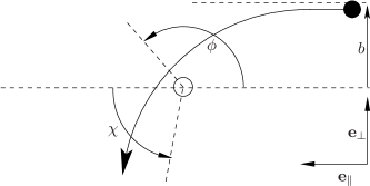
Figure 1: Trajectory of a particle in a two body collision in the cent-re of mass frame, with definition of the relevant quantities for its analysis, notably the deflection angle $\chi$.

In the center of mass frame, the collision occurs as depicted in Fig. 1, which shows the definition of the impact factor $b$, and the deflection angle $\chi=2\phi-\pi$. As energy is conserved in the collision, the magnitudes of the initial and final relative velocity, $V=|{\mathbf{V}}|$, are equal. It follows that

$$\frac{\Delta V_{\perp}}{V} =-\sin(\chi)$$ (10a)

$$\frac{\Delta V_{\parallel}}{V} =1-\cos(\chi).$$ (10b)

The angle $\phi$ can be calculated, as a function of the impact factor $b$, using the classic formula Landau and Lifshitz (1976)

$$\phi(b)=\int_{r_{min}}^{\infty}\frac{(b/r^{2})dr}{\sqrt{1-(b/r)^{2}-4v(r)/mV^{2}}},$$ (11)

where $r_{min}$ is the positive root of the denominator.

We consider now the case of a pure decaying power law pair potential,

$$v(r)=-\frac{g}{r^{\gamma}}$$ (12)

and $\gamma>0$. For $g>0$ the corresponding force is attractive, while $g<0$ it is repulsive. In what follows we will consider the attractive case, but we will discuss below also the repulsive case. Indeed it turns out that our essential results hold in both cases.

The integral (11) leads naturally to the definition of the characteristic length scale

$$b_{0}=\left(\frac{2|g|}{mV^{2}}\right)^{1/\gamma}\,.$$ (13)

Considering the attractive case, Eq. (11) may then be rewritten as

$$\phi(b)=\int_{r_{min}}^{\infty}\frac{(b/r^{2})dr}{\sqrt{1-(b/r)^{2}+2(b_{0}/r)^{\gamma}}}\,.$$ (14)

Changing to the variable $x=b/r$, we obtain

$$\phi(b/b_{0})=\int_{0}^{x_{max}}\frac{dx}{\sqrt{1-x^{2}+2(b_{0}/b)^{\gamma}x^{\gamma}}},$$ (15)

where now $x_{max}$ is the positive root of the denominator. Since $x_{max}$, for given $\gamma$, is a function of $b/b_{0}$ only, it follows that $\phi$ is also a function of $b/b_{0}$ only.

Equation (14) can be solved analytically only in a few cases, and notably for the case $\gamma=1$ which corresponds to gravity in $d=3$. For the general ($\gamma\neq 1$) case, the integral can easily be computed numerically, and $\frac{\Delta V_{\perp}}{V}$ and $\frac{\Delta V_{\parallel}}{V}$ can then be calculated. Figure 2 displays the results for a few chosen cases. In order to derive analytically the parametric dependences of the two body relaxation rate, it suffices, as we will see, to have analytical approximations in the two asymptotic regimes of soft ($b/b_{0}\gg 1$) and hard ($b/b_{0}\ll 1$) collisions. The corresponding expressions have been derived in a separate article Chiron and Marcos (2015) by one of us (BM) and another collaborator. In what follows we make use of the relevant results of Chiron and Marcos (2015), where the full details of their derivations may be found.

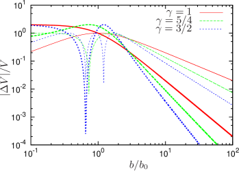
Figure 2: Absolute value of relative change in the perpendicular (thin lines) and parallel (thick lines) components of the relative velocity in a two body encounter, for different attractive power-law potentials. The behaviors at small and large values of $b/b_{0}$ are well described by the analytical expressions given in the text.

II.1.1 Soft collisions ($b\gg b_{0}$)

When $b\gg b_{0}$ the particle trajectories are weakly perturbed, and the collision is said to be soft. It is shown in Chiron and Marcos (2015) that, in this region, one has

$$\chi(b/b_{0})=2A(\gamma)(b_{0}/b)^{\gamma}+\mathcal{O}((b_{0}/b)^{2\gamma}),$$ (16)

where

$$A(\gamma)=\sqrt{\pi}\frac{\Gamma\left(\frac{\gamma+1}{2}\right)}{\Gamma\left(\frac{\gamma}{2}\right)}\,,$$ (17)

with $\Gamma(x)$ being the Euler Gamma function. As the angle of deflection $\chi\ll 1$, it follows that

$$\frac{\Delta V_{\perp}}{V} =-2A(\gamma)\left(\frac{b_{0}}{b}\right)^{\gamma}+\mathcal{O}((b_{0}/b)^{2\gamma})$$ (18a)

$$\frac{\Delta V_{\parallel}}{V} =2A(\gamma)^{2}\left(\frac{b_{0}}{b}\right)^{2\gamma}+\mathcal{O}((b_{0}/b)^{4\gamma}).$$ (18b)

In Appendix A an alternative derivation of Eq. (18a) is presented.

II.1.2 Hard collisions ($b\ll b_{0}$)

It is shown in Chiron and Marcos (2015) that, in this asymptotic regime,

$$\chi(b/b_{0})=\,\frac{\gamma\pi}{2-\gamma}+\mathcal{O}\left((b/b_{0})^{\alpha}\right),$$ (19)

where $\alpha=2\gamma/(2-\gamma)$ for $\gamma<2/3$, $\alpha=b/b_{0}\ln\left(b_{0}/b\right)$ for $\gamma=2/3$ and $\alpha=1$ for $2/3<\gamma<2$. If $\gamma\geq 2$, collisions are well defined with an asymptotic free state Chiron and Marcos (2015) only if

$$b>\beta b_{0},$$ (20)

where

$$\beta=\gamma^{1/\gamma}\left(1-\frac{2}{\gamma}\right)^{\frac{2-\gamma}{2\gamma}}.$$ (21)

For $b\leq\beta b_{0}$, on the other hand, there is a finite time singularity, i.e., the relative distance of the particles vanishes at a finite time.

The first term in the asymptotic expansion Eq. (19) gives the angle of deflection in the limit of arbitrarily small impact factors, and shows that it depends on $\gamma$. While for the case $\gamma=1$ (i.e. gravity in $d=3$) each particle velocity is exactly reversed in the center of mass frame ($\chi=\pi$), the general result for the deflection angle is different, and it increases to infinity as $\gamma\rightarrow 2$ from below. At $\gamma=4/3$ each particle performs one full loop around the center of mass and escapes asymptotically in the same direction it arrived in, at $\gamma=12/7$ each particle performs two full loops etc., and as $\gamma\rightarrow 2$ from below the number of such loops diverges.

For $\gamma\geq 2$, as noted, there is in fact a singularity, with the particles running into one another at a finite time. To include this case in our treatment we must therefore assume that the pair potential Eq. (12) is regularized at $r=0$, so that there is a well defined collision for any impact factor. It follows from our analysis that this means that the asymptotic behavior below some arbitrarily small scale must be either repulsive, or, if attractive, diverging more slowly that $1/r^{2}$. In what follows this assumption will suffice to extend our results to the range $\gamma\geq 2$.

II.2 Computation of the cumulative effect of many collisions

Following Chandrasekhar we assume that thermal relaxation is induced by the randomization of particles velocity by two body collisions. In order to estimate the accumulated effect of two body collisions on a particle as it crosses the whole system, we estimate first the number of encounters per unit of time with impact parameter $b$. In doing so we make the following approximations:

1. the system is treated as a homogeneous random distribution of particles in a $d$ dimensional sphere of radius $R$,

2. the initial squared relative velocity of colliding particles is given by the variance of the particle velocities in the system.

Each particle is then assumed to perform a simple homogeneous random walk in velocity space, with zero mean change in velocity (because the deflections due to each encounter have no preferred direction), and a positive mean squared velocity which we determine below. In this approximation, we assume that the particles have rectilinear trajectories. This approximation clearly breaks down in the case of hard collisions, in which the trajectory is strongly perturbed. We expect however the estimation of the number of collisions per unit of time to remain correct in this case, because encounters modify only the direction of the velocity, and not its modulus.

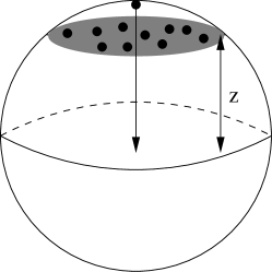
Figure 3: The system is approximated as a perfectly spherical distribution of particles with radius $R$.

As illustrated schematically in Fig. (3), we now divide the system in disks of thickness $dz$, and write the average number of encounters with impact parameter between $b$ and $b+db$ of a particle crossing this disk as

$$\delta n=\frac{B_{d}N}{R^{d}}b^{d-2}\,db\,dz$$ (22)

where $B_{d}$ is a numerical factor which depends on the spatial dimension $d$ (e.g. $B_{2}=2/\pi$, $B_{3}=3/2$).

Multiplying Eq. (22) by the square of Eq. (10) with the condition (15), and integrating from $z=0$ to $z=R$ and from $b=0$ to $b=\sqrt{R^{2}-z^{2}}$, we then estimate the average change in the velocity during one crossing of the system, for the perpendicular and parallel components of the velocity respectively, as:

$$\frac{\langle|\Delta V_{\perp,\parallel}^{2}|\rangle}{|V^{2}|}=2B_{d}N\left(\frac{b_{0}}{R}\right)^{d-1}\,{\mathcal{I}}_{\perp,\parallel}\left(\frac{b_{0}}{R}\right)$$ (23)

where

$${\mathcal{I}}_{\perp,\parallel}(x_{R})=\int_{0}^{x_{R}}dx\,x^{d-2}\,\Theta_{\perp,\parallel}(x)\,\sqrt{1-\frac{x^{2}}{x_{R}^{2}}}$$ (24)

where $x=b/b_{0}$, $x_{R}=R/b_{0}$ and

$$\Theta_{\perp}(x) =\sin^{2}\left(\chi(x)\right)$$ (25a)

$$\Theta_{\parallel}(x) =\left[1-\cos(\chi(x))\right]^{2}.$$ (25b)

Writing the expression for $\frac{\langle|\Delta V_{\perp,\parallel}^{2}|\rangle}{|V^{2}|}$ in this way allows a simple and useful comparison with the case of particles interacting by an exact repulsive hard core potential. Indeed it is straightforward to show (see e.g. Balescu (1997)) that for (infinitely) hard particles with a diameter $\sigma$, one has

$$\chi(b)=\left\{\begin{array}[]{ll}2\arccos\left(\frac{b}{\sigma}\right)&\text{if }b\leq\sigma\\ 0&\text{otherwise.}\end{array}\right.$$ (26)

Calculating $\frac{\langle|\Delta V_{\perp,\parallel}^{2}|\rangle}{|V^{2}|}$ for this case using exactly the same approach used above, one obtains, for the case $\sigma=b_{0}$, exactly Eq. (23) with

$${\mathcal{I}}_{\perp} =\frac{8}{(d+3)(d+1)}$$ (27a)

$${\mathcal{I}}_{\parallel} =\frac{4}{d-1}{\mathcal{I}}_{\perp}.$$ (27b)

Let us return now to the expressions Eq. (24) for the case of (attractive) power law interactions. Given that $x_{R}\gg 1$ we can make the approximation

$${\mathcal{I}}_{\perp,\parallel}(x_{R}) \approx\int_{0}^{1}dx\,x^{d-2}\,\Theta_{\perp,\parallel}(x)$$ (28)

$$+ \int_{1}^{x_{R}}dx\,x^{d-2}\,\Theta_{\perp,\parallel}(x)\,\sqrt{1-\frac{x^{2}}{x_{R}^{2}}}.$$

The first integral gives the contribution due to hard collisions ($b<b_{0}$). It is finite provided only that the deflection angle is well defined, i.e., provided only that the two body collisions is well defined. As we have discussed above this is true for any $\gamma<2$, and for $\gamma\geq 2$ if we assume the singularity at $r=0$ to be appropriately regularized. Thus this term gives a contribution to $\frac{\langle|\Delta V_{\perp,\parallel}^{2}|\rangle}{|V^{2}|}$ which has precisely the parametric dependences of an exact repulsive hard core, differing only by an overall numerical factor.

Considering now the second term, giving the contribution from soft collisions ($b>b_{0}$), we see that there are two different cases according to the large $x$ behavior of $\Theta_{\perp,\parallel}$: the integral is convergent as $x_{R}\rightarrow\infty$ if and only if $x^{d-1}\Theta_{\perp,\parallel}(x)\rightarrow 0$ as $x\rightarrow\infty$. We thus infer from Eqs. (18) the following:

• For $0<\gamma<(d-1)/2$,

  $${\mathcal{I}}_{\perp}(x_{R}) \approx 4A^{2}(\gamma)\int_{0}^{x_{R}}dx\,x^{d-2-2\gamma}\,\sqrt{1-\frac{x^{2}}{x_{R}^{2}}}$$ (29)

  $$= A^{2}(\gamma)\sqrt{\pi}\frac{\Gamma\left[d/2-1/2-\gamma\right]}{\Gamma\left[d/2+1\gamma\right]}x_{R}^{d-1-2\gamma}$$ (30)

  and ${\mathcal{I}}_{\parallel}(x_{R})\ll{\mathcal{I}}_{\perp}(x_{R})$. Thus the integral is dominated by the contribution of soft scatterings, for which the change in the relative velocity is predominantly orthogonal to the initial relative velocity. Replacing Eq. (29) in Eq. (23), we obtain the scaling

  $$\frac{\langle|\Delta{\mathbf{V}}^{2}|\rangle}{V^{2}}\approx\frac{\langle|\Delta V_{\perp}^{2}|\rangle}{|V^{2}|}\sim N\left(\frac{b_{0}}{R}\right)^{2\gamma}.$$ (31)

  where

  $$\frac{\langle|\Delta{\mathbf{V}}|^{2}\rangle}{V^{2}}=\frac{\langle|\Delta{\mathbf{V}}_{\perp}|^{2}\rangle}{V^{2}}+\frac{\langle|\Delta{\mathbf{V}}_{\parallel}|^{2}\rangle}{V^{2}}.$$ (32)

• For $\gamma=(d-1)/2$, which corresponds to gravity in $d=3$, the contribution from all impact factors from the scale $b_{0}$ must be included and

  $${\mathcal{I}}_{\perp}(x_{R})\approx 4A^{2}(\gamma)\ln\,x_{R}\,.$$ (33)

  As in the previous case, ${\mathcal{I}}_{\parallel}(x_{R})\ll{\mathcal{I}}_{\perp}(x_{R})$. Note that, given $x_{R}\gg 1$ this result for ${\mathcal{I}}_{\perp}(x_{R})$ is very insensitive to precisely where the lower cut-off at $b\sim b_{0}$ is chosen. We obtain therefore

  $$\frac{\langle|\Delta{\mathbf{V}}^{2}|\rangle}{|V^{2}|}\sim N\left(\frac{b_{0}}{R}\right)^{d-1}\ln\left(\frac{R}{b_{0}}\right).$$ (34)

• For $\gamma>(d-1)/2$, we have

  $${\mathcal{I}}_{\perp,\parallel}(x_{R})\approx{\mathcal{I}}_{\perp,\parallel}(\infty)\approx\int_{0}^{\infty}dx\,x^{d-2}\,\Theta_{\perp,\parallel}(x)$$ (35)

  which is a constant that can be numerically calculated in a straightforward way for any given pair potential in this class. We obtain therefore

  $$\frac{\langle|\Delta{\mathbf{V}}^{2}|\rangle}{V^{2}}\sim N\left(\frac{b_{0}}{R}\right)^{d-1}.$$ (36)

In the last case, for sufficiently rapidly decaying potentials, we obtain therefore the same scaling as for the case of hard core particles of diameter $b_{0}$.

II.3 Scalings with $N$ of the relaxation rate in a QSS

Using these results, we now determine how the relaxation rate scales with the parameters of the system. Assuming the system to be in a QSS we can then obtain its scaling as a function of $N$ alone. For clarity we drop irrelevant numerical prefactors, but these will be analyzed further in Sect. VI.

We define the relaxation rate $\Gamma$ as the inverse of the time scale at which the normalized average change in velocity squared due to collisions is equal to one. Given that the estimated $\frac{\langle|\Delta{\mathbf{V}}|^{2}\rangle}{V^{2}}$ is the average change in a crossing time $\tau_{dyn}$, we have therefore

$$\Gamma\tau_{dyn}\simeq\frac{\langle|\Delta{\mathbf{V}}|^{2}\rangle}{V^{2}}\,.$$ (37)

In order to obtain the scaling with $N$ from the above results, we need to determine how the ratio $b_{0}/R$ scales with $N$. Using the definition Eq. (13) and assuming, as stated above, that the modulus of the relative velocity of colliding particles can be taken to be of the same order as the typical velocity of a single particle $v$, we have

$$\left(\frac{b_{0}}{R}\right)^{\gamma}\sim\frac{g}{mv^{2}R^{\gamma}}\sim\frac{1}{N}\frac{gN^{2}}{(mNv^{2})R^{\gamma}}\sim\frac{1}{N}\frac{U}{K}$$ (38)

where $K$ is the total kinetic energy and $U$ the total potential energy of the system.

If we now assume the system to be in a QSS, i.e. in virial equilibrium, the virial theorem gives that

$$2K+\gamma U=3PV,$$ (39)

where $P$ is the pressure of the particles on the boundaries if the system is enclosed, and $P=0$ if the system is open.

By definition the mean-field scaling with $N$ makes each term in Eq. (39) scale in the same way with $N$ so that the relation remains valid independently of $N$ (up to finite $N$ fluctuations). Thus using this scaling we can infer that

$$b_{0}\sim RN^{-1/\gamma}.$$ (40)

Using Eqs. (31), (34) and (36), we then infer the following behaviors:

• For $0<\gamma<(d-1)/2$,

  $$\Gamma\,\tau_{dyn}\sim N(b_{0}/R)^{2\gamma}\sim N^{-1}.$$ (41)

• For $\gamma=(d-1)/2$

  $$\Gamma\,\tau_{dyn}\sim N^{-1}\ln\left(N\right).$$ (42)

• For $\gamma>(d-1)/2$

  $$\Gamma\,\tau_{dyn}\sim N^{-(d-1-\gamma)/\gamma}.$$ (43)

It follows that that the condition Eq. (6) only holds for potentials with $\gamma<d-1$. Only in this case therefore can the QSS be supposed to exist as we have assumed. For $\gamma\geq d-1$, on the other hand, the relaxation induced by two body collisionality occurs on a time scale which is short compared to a particle crossing time, and a stationary non-thermal state cannot exist on the latter time scale, i.e., a QSS cannot exist.

II.4 Relaxation rates for softened power-law potentials

We consider now the case in which the power-law potential is “softened” at short distances, i.e., regulated so that the modulus of the force between two particles is bounded above at some finite value. The principle motivation for considering this case here is that, in practice, even for $\gamma<2$, we are unable numerically to test directly the validity of the scaling predictions Eqs. (36)-(41) for the exact (singular) potentials: the numerical cost of integrating sufficiently accurately hard two body scatterings over the long time scales required is prohibitive. Instead we will consider power-law potentials softened at a scale $\epsilon$, and study the scaling with both $N$ and $\epsilon$ of the relaxation rates in the numerically accessible range for these parameters.

A detailed analysis of the two body scattering for such softened power law potentials has been given also in Chiron and Marcos (2015). We again use the results of this paper to infer, using Eqs. (23)-(25) above, the parametric scalings of the relaxation rate. As in the previous section, we defer until later a discussion of the exact numerical factors, for the specific smoothing functions used in our numerical simulations.

As softening modifies the force below a characteristic scale $\epsilon$, its effect is to modify the deflection angles for impact factor $b$ below a scale of the same order. From the considerations above it is then evident that, for $\epsilon<b_{0}$, such a softening does not change the parametric scalings: it can only change the numerical value of the (finite) first integral in Eq. (28). For $\epsilon>b_{0}$, on the other hand, the second integral in Eq. (28) is modified because the functions $\Theta_{\perp,\parallel}$ are modified up to $x\sim\epsilon/b_{0}$. Assuming that $\epsilon\ll R$, this will lead to a modification of the parametric scaling of the full expressions for $\frac{\langle|\Delta{\mathbf{V}}|^{2}\rangle}{V^{2}}$ when $\gamma\geq(d-1)/2$. In Chiron and Marcos (2015) it is shown that, when $\epsilon\geq b_{0}$, the deflection angle can be approximated as

$$\chi\simeq\left\{\begin{array}[]{ll}2B(\gamma)\left(\frac{b_{0}}{\epsilon}\right)^{\gamma}\left(\frac{b}{\epsilon}\right)&\text{if }b<\epsilon^{*}\\ 2A(\gamma)\left(\frac{b_{0}}{b}\right)^{\gamma}&\text{if }b>\epsilon^{*},\end{array}\right.$$ (44)

where $B(\gamma)$ is a finite constant the exact value of which depends on the functional form of softening used (and $A(\gamma)$ is as defined in Eq. (17)). The scale $\epsilon^{*}$ is of the same order as $\epsilon$ (from continuity of Eq. (44) at $b=\epsilon^{*}$, their ratio is given by $\epsilon^{*}/\epsilon\sim(A/B)^{\frac{1}{1+\gamma}}$).

Using Eq.(44) we can now calculate approximately the second integral in Eq. (28) for the cases in which the parametric dependence of their values are modified by the smoothing (with $\epsilon>b_{0}$):

• For $\gamma>(d-1)/2$ (taking $x_{R}\to\infty$):

  $${\mathcal{I}}_{\perp} \simeq\left[\frac{B^{2}(\gamma)}{d+1}+\frac{A^{2}(\gamma)}{2\gamma-d+1}\right]\left(\frac{\epsilon}{b_{0}}\right)^{d-1-2\gamma}$$ (45a)

  $${\mathcal{I}}_{\parallel} \simeq\left[\frac{B^{4}(\gamma)}{4(d+3)}+\frac{A^{4}(\gamma)}{4\gamma+1-d}\right]\left(\frac{\epsilon}{b_{0}}\right)^{d-1-4\gamma}.$$ (45b)

  and therefore ${\mathcal{I}}_{\perp}\gg{\mathcal{I}}_{\parallel}$ if $\epsilon\gg b_{0}$.

• For $\gamma=(d-1)/2$, assuming $x_{R}\gg(\epsilon/b_{0})$ (i.e. $\epsilon\ll R$), we obtain

  $${\mathcal{I}}_{\perp}\simeq A^{2}(\gamma)\ln\left(\frac{R}{\epsilon}\right)\,,$$ (46)

  while ${\mathcal{I}}_{\parallel}$ is given as Eq. (45b), and ${\mathcal{I}}_{\perp}\gg{\mathcal{I}}_{\parallel}$ if $\epsilon\gg b_{0}$.

Using these results we infer finally that the scalings of the relaxation rates of a QSS (with $b_{0}$ scaling as in Eq.  (40)) in the large $N$ limit are the following:

• If $0<\gamma<(d-1)/2)$,

  $$\Gamma\,\tau_{dyn}\sim N^{-1},$$ (47)

  i.e. the same as in the absence of smoothing;

• If $\gamma>(d-1)/2$, then

  $$\Gamma\,\tau_{dyn}\sim N^{-1}\left(\frac{\epsilon}{R}\right)^{d-1-2\gamma}$$ (48)

• If $\gamma=(d-1)/2$, then

  $$\Gamma\,\tau_{dyn}\sim N^{-1}\ln\left(\frac{R}{\epsilon}\right).$$ (49)

In summary, the correct parametric scaling for the two body relaxation rates of a QSS, in the case of a power-law potential softened at a scale $\epsilon>b_{0}$, are well approximated by simply introducing a cutoff at an impact factor of order $\epsilon$ (and therefore considering only the contribution from soft collisions).

For what concerns the existence of QSS, we thus conclude that, with a softened power law potential, one can satisfy the condition Eq. (6) even for any $\gamma\geq d-1$. Indeed, taking $\epsilon/R$ to be independent of $N$ (i.e. scaling the softening with the system size), we obtain in all cases that $\Gamma_{\epsilon}\,\tau_{dyn}\sim N^{-1}$. More generally, it is straightforward to deduce what scaling of $\epsilon$ with $N$ is required to satisfy the condition Eq. (6) in the mean-field limit.

III Numerical simulations

We have performed numerical simulations in $d=3$ of the evolution of $N$ particle systems, extending to sufficiently long times to observe their collisional evolution. As we have discussed in the previous section, exact power law interactions with $\gamma\geq(d-1)/2$ lead to strong collisions at impact factors $b<b_{0}$. Indeed, as we have seen, when $\gamma$ increases much above unity particles can even make multiple loops around one another during collisions (cf. Eq. (19)). The smaller is $b$, the shorter is the characteristic time for a collision compared to the mean field time and therefore the greater is temporal resolution required for an accurate integration (and, in particular, conservation of the energy). This means it is too expensive numerically, even for a few thousand particles, to accurately simulate such a system for times long enough to be comparable to the predicted relaxation times. Indeed we have seen that the calculation we have done predicts that, even for $(d-1)/2<\gamma<d-1$ (i.e. $1<\gamma<2$ in $d=3$), relaxation should be dominated by strong collisions with $b\sim b_{0}$ but nevertheless $\Gamma\,\tau_{dyn}$ diverges in the mean field limit.

For these reasons, we employ a potential with a softening which is sufficiently large to suppress strong collisions. The predicted scalings we can test are thus those given in Sect. II.4, rather than the ones corresponding to pure power-law potentials given in Sect. II.3. By studying also the scalings with the softening $\epsilon$ at fixed $N$, however, we can indirectly test in this way the extrapolation to the scalings in Sect. II.3.

III.1 Code

We use a modification of the publicly available gravity code GADGET2Springel (2005). The force is computed using a modified Barnes and Hut tree algorithm, and we have modified the code in order to treat pair potentials of the form Eq. (1) and softened versions of them (which are those we use in practice). We use an opening angle $\theta=0.001$, which ensures a very accurate computation of the force. The evolution of the system is computed using a Verlet-type Drift-Kick-Drift symplectic integration scheme. The simulations are checked using simple convergence tests on the numerical parameters, and their accuracy is monitored using energy conservation. For the time-steps used here it is typically conserved to within $0.1\%$ over the whole run, orders of magnitude smaller than the typical variation of the kinetic or potential energy over the same time.

III.2 Initial and boundary conditions

As initial conditions we take the $N$ particles randomly distributed in a sphere of radius $R=1/2$, and ascribe velocities to particles so that each component is an independent uniformly distributed variable in an interval $[-\xi,\xi]$ (i.e. “waterbag” type initial conditions in phase space). The parameter $\xi$ is chosen so that initial virial ratio is unity, i.e., $2K/|U|=\gamma$. We make this choice of initial conditions because it is expected to be close to a QSS, to which (collisionless) relaxation should occur “gently”, and this is indeed what we observe. We have chosen to enclose the system in a cubic box of size $L=1$, in order to avoid the complexities associated with particle evaporation. This constraint is imposed in practice using soft boundary conditions, which are implemented by changing the sign of the $i^{th}$ component of the velocity when the $i^{th}$ component of the position lies outside the simulation box. We use a time step of the order of $10^{-3}\tau_{dyn}$ (which provides well converged results), where $\tau_{dyn}$ is defined precisely below.

III.3 Softening

We have performed simulations using two different softening schemes: a “compact” softening and a “Plummer” softening. The former corresponds to a two body potential

$$v^{\text{C}}(r,\epsilon)=\left\{\begin{array}[]{ll}-\frac{g}{r^{\gamma}}&\text{if }r\geq\epsilon\\ -\frac{g}{\epsilon^{\gamma}}{\text{v}}\left(r/\epsilon\right)&\text{if }0\leq r\leq\epsilon,\end{array}\right.$$ (50)

where ${\text{v}}(x)$ is a polynomial, of which the exact expression is given in App. B. It is chosen so that the potential and its first two derivatives are continuous at $r=\epsilon$, and it interpolates to a force which vanishes at $r=0$ via a region in which the force becomes repulsive. The Plummer smoothing corresponds to the simple potential

$$v_{\epsilon}^{P}(r)=-\frac{g}{(r^{2}+\epsilon^{2})^{\gamma/2}},$$ (51)

which is everywhere attractive.

As we have noted it is straightforward to calculate numerically the relaxation rates for these softened potentials, using Eq. (11) and Eq. (23). We show in Fig. 4 the ratio of the resultant $\frac{\langle|\Delta{\mathbf{V}}_{\perp}^{2}|\rangle}{\langle|V^{2}|\rangle}$ compared to its value for the exact power law, for $\gamma=5/4$ and $\gamma=3/2$, as a function of the ratio $\epsilon/b_{0}$. As described in the previous section we observe that, for $\epsilon\ll b_{0}$, the effect of the softening is negligible, while for $\epsilon\gg b_{0}$, we recover a simple power law scaling with $\epsilon$ which agrees with that derived above for this regime, cf. Eq. (48). We note that in Fig. 4 the normalization for the asymptotic Plummer curves is greater that for the compact softening.

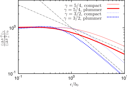
Figure 4: Numerical evaluation of Eqs. (11) and Eq. (23) normalized to the value for $\epsilon/b_{0}\to 0$ for $\gamma=5/4$ and $\gamma=3/2$. The power-law lines are the theoretical scaling (48).

Performing simulations with these two different softening schemes allows us to test not just the robustness of the agreement with the theoretical scalings derived above, which should not depend on the details of the softening scheme. It also allows to test more quantitatively for the correctness of the theoretical predictions for the relaxation rates, which predicts also the relative amplitude of the relaxation rate in the regime $\epsilon\gg b_{0}$. To facilitate this comparison it is convenient to define an effective softening $\epsilon_{eff}$ obtained by assuming that all the collisions are soft, i.e.,

$$\chi_{\epsilon}\simeq\left\{\begin{array}[]{ll}0&\text{if }b<\epsilon_{eff}\\ 2A(\gamma)\left(\frac{b_{0}}{b}\right)^{\gamma}&\text{if }b\geq\epsilon_{eff}.\end{array}\right.$$ (52)

Computing the same quantity as in Fig. (4), we can determine, by matching with the result for any other softening scheme, a value of $\epsilon_{eff}$ in units of $\epsilon$. We can compute therefore an effective softening using

$$\epsilon_{eff}=\alpha\,\epsilon\,,$$ (53)

where the values of $\alpha$ are given in Tab. 1 for our two softening schemes, for the values of $\gamma$ we explore here (in the range $\gamma\geq 1$ where the softening plays a role). The result for the case of gravity and the Plummer softening is in agreement with that derived in Theis (1998) (see also White (1978)).

Thus our analytical calculations predict that the relaxation rates of QSS measured with the different softening schemes should not only scale in the same way as a function of $\epsilon$ (for $\epsilon\gg b_{0}$) but also they should be equal at values of $\epsilon$ corresponding to the same $\epsilon_{eff}$.

$\gamma$	compact core	plummer core
1	0.80	1.69
5/4	0.74	1.55
3/2	0.75	1.50

Table 1: Factor $\alpha$ (see Eq. (53)) to compute the effective softening $\epsilon_{eff}$ (see text) in units of $\epsilon$, for the two different softening schemed used in this work.

III.4 Sets of simulations

We performed, for each value of $\gamma$, and each softening scheme, two different kinds of sets of simulations. One set is at fixed particle number $N$ and a range of different values of the softening $\epsilon$, while in the other set $\epsilon$ is kept constant and $N$ is varied. To refer to the simulations we will use the notation $\mathcal{C}(\gamma;N,\epsilon)$ for a simulation with the compact (“$\mathcal{C}$”) softening (1), power law exponent $\gamma$, particle number $N$ and softening $\epsilon$. Similarly we denote $\mathcal{P}(\gamma;N,\epsilon)$ a set of simulations with the Plummer (“$\mathcal{P}$”) smoothing.

The simulations on which our results below are based are the following:

• A set $\mathcal{C}(\gamma;N=8000,\epsilon)$ for $\gamma=1/2$, $\gamma=1$ , $\gamma=5/4$ and $\gamma=3/2$ with the values of $\epsilon$ listed in the first column of Tab. 2.

• A set $\mathcal{C}(\gamma;N,\epsilon/L=0.005)$ for $\gamma=1/2$, $\gamma=1$ , $\gamma=5/4$ and $\gamma=3/2$ with the values of $N$ listed in the third column of Tab. 2.

• A set $\mathcal{P}(\gamma;N=8000,\epsilon)$ for $\gamma=5/4$ and $\gamma=3/2$ with the values of $\epsilon$ listed in the second column of Tab. 2.

• A set $\mathcal{P}(\gamma;N,\epsilon/L=0.005)$ for $\gamma=5/4$ and $\gamma=3/2$ with the values of $N$ listed in the third column of table Tab. 2.

$\epsilon/L$	0.0005  0.001   0.002   0.003   0.004   0.005
	0.01   0.02   0.03   0.04
$N$	$10^{3}$   $12^{3}$   $16^{3}$   $20^{3}$   $26^{3}$   $30^{3}$

Table 2: List of simulations: The first row gives the values of the softening parameter $\epsilon$ used in two sets of simulations with $N=8000$ particles; the second column gives the values of $N$ employed in two sets of simulations at fixed $\epsilon/L=0.005$.

III.5 Numerical estimation of the relaxation rate

To measure numerically the relaxation rate of a QSS we study the temporal evolution of different quantities. We consider principally two quite different quantities. On the one hand the total kinetic (or potential) energy of the system, and on the other hand, the averaged quantity defined as

$$\Delta(t)\equiv\frac{\langle(e(t)-e(t^{*}))^{2}\rangle}{2k^{2}(t^{*})}\,,$$ (54)

where $e(t)$ is the total energy of a single particle (at time $t$), and $k(t)$ is the kinetic energy per particle. The time $t^{*}$ is an initial chosen time (and thus $t>t^{*}$) at which the system has relaxed, starting from the initial condition, to a QSS (typically we have below of $t^{*}\sim 10\,\tau_{dyn}$). The brackets $\left<\cdot\right>$ indicate an average over all the particles in the system.

While the first quantity probes simply the macroscopic evolution of the system in a “blind” manner, the second quantity probes more directly the microscopic evolution of the quantities considered in the theoretical calculation. Indeed the calculation in Sect. II.1 provides a prediction for the average variation of the velocity of particles due to collisions. The difficulty with measuring this directly is that the velocity of particles also changes also continuously because of the mean field potential. Particle energy, on the other hand, remains exactly constant in a QSS, and its change is in principle due to collisional effects, which we posit here are dominated by the two body collisions.

III.6 Other indicators of relaxation

In order to determine whether the system is in a QSS state (and hence not in thermal equilibrium), we compute moments of the system’s velocity distribution. If the system is at thermal equilibrium, the probability distribution of velocities must be Gaussian for each component with zero mean, and therefore all odd moments of such components must vanish, while even moments of order higher than two are determined as a simple power of the variance:

$$\langle v_{i}^{2n}\rangle=(2n-1)!!\langle v_{i}^{2}\rangle^{n}\,,$$

In order to detect the deviation from Gaussianity of the velocity distribution we use the first two even moments of order larger than two, normalized so that they are zero in the case of Gaussianity:

$$\phi_{4} = \frac{\overline{\langle v_{i}^{4}\rangle}}{3\overline{\langle v_{i}^{2}\rangle}^{2}}-1$$ (55)

$$\phi_{6} = \frac{\overline{\langle v_{i}^{6}\rangle}}{15\overline{\langle v_{i}^{2}\rangle}^{3}}-1\,,$$ (56)

where $\overline{\cdot}$ denotes average over the coordinates.

III.7 Units

As noted above we take the side of the enclosing box $L=1$. The mean field characteristic time is defined (following Eq. (5)) as:

$$\tau_{dyn}=\sqrt{\frac{mL^{\gamma+2}}{gN}}\,$$ (57)

and we report our results for velocities in units of

$$v^{*}=\frac{L}{\tau_{dyn}}=\sqrt{\frac{gN}{mL^{\gamma}}}.$$ (58)

IV Results for case of gravity ($\gamma=1$)

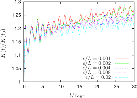
(a)

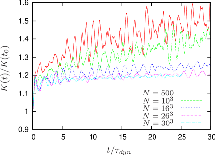
(b)

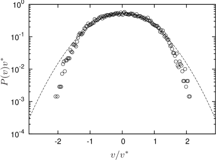
(c)

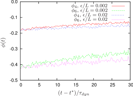
(d)

(e)

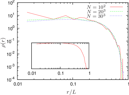
(f)

Figure 5: Results of simulations for the case of gravity ($\gamma=1$): (a) Evolution of the total kinetic energy normalized to its initial value, for $N=8000$ and different values of $\epsilon$, i.e., the set of simulations $\mathcal{C}(1;8000,\epsilon/L)$; (b) evolution of the normalized total kinetic energy with $\epsilon=0.01$ and a range of different values of $N$, i.e., the set of simulations $\mathcal{C}(1;N,0.01)$; (c) velocity distribution for the simulation $\mathcal{C}(1;8000,0.002)$ at $t=20\tau_{dyn}$ and (d) evolution of $\phi_{4}$ and $\phi_{6}$ for the simulations $\mathcal{C}(1;8000,0.002)$ and $\mathcal{C}(1;8000,0.02)$ at $t=20\tau_{dyn}$, (e) density distribution for the simulations $\mathcal{C}(1;8000,\epsilon)$ at varying $\epsilon$ and $t=20\tau_{dyn}$; (f) density distribution for the simulations $\mathcal{C}(1;i,0.01)$ at $t=20\tau_{dyn}$ and (inset) the same quantity for the simulation $\mathcal{C}(1;30^{3},0.01)$ in log-log scale (note the density drops rapidly at $R/L\approx 1/3$).

In this section we check our numerical and analytical results using the canonical much studied case of gravity as an established benchmark.

IV.1 Qualitative inspection of evolution

Fig. 5a shows the evolution of the total kinetic energy normalized to its initial value at $t=0$, for different values of the softening $\epsilon$ simulated. We observe that, for sufficiently small softening, and sufficiently short times, the curves match very well: we interpret this to be because they are following the same mean-field evolution. Further the kinetic energy (and viral ratio) shows a rapid relaxation (by $t\approx\tau_{dyn}$) to relatively small and progressively damped oscillations around an approximately stationary value. This is the familiar mean-field relaxation to a QSS, which in practice we will consider to be established below from $t\approx 10\tau_{dyn}$. For larger times we observe a slow linear drift in time of the average value of the kinetic energy, which can be interpreted as a signature of the slow collisional relaxation process. As predicted by Eq. (49), the collisional relaxation is suppressed increasing the softening.

Fig. 5b compares the evolution of systems with a fixed (compact) softening but different number of particles. We observe a similar behavior to that in the previous plot, and very consistent with the interpretation given of this evolution as the relaxation to a QSS: we observe a drift away from the almost stationary kinetic energy which develops more slowly as the number of particles $N$ increases.

Fig. 5c shows, for the simulation $\mathcal{C}(1;8000,0.002)$, the velocity distribution at $t=20\tau_{dyn}$. We observe that the tails of the distribution are clearly non-Gaussian, and thus that the system is not at thermal equilibrium. This is confirmed by the evolution of the functions $\phi_{4}$ and $\phi_{6}$, which are plotted in Fig. 5d. They are clearly non-zero, indicating a non-Gaussian state, and further, show manifestly a slow growth on a longer time-scale which is indicative of an evolution towards a thermal state. Finally, as shown in Fig. 5e and 5f respectively, the density profile (i.e. mean density in spherical shells centered on the center of mass of the system) at $t=20\tau_{dyn}$ are substantially independent of the parameters $\epsilon$ and $N$, as they should be if this profile is characteristic of a QSS.

IV.2 Scaling of the relaxation rate

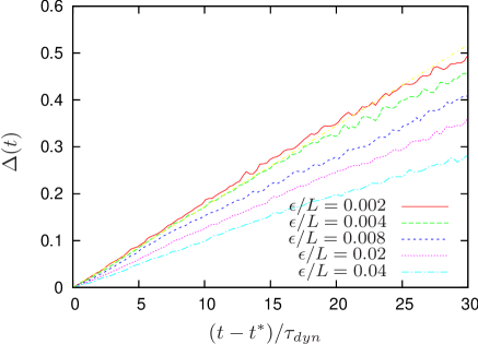
(a)

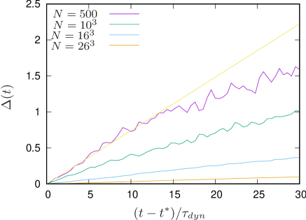
(b)

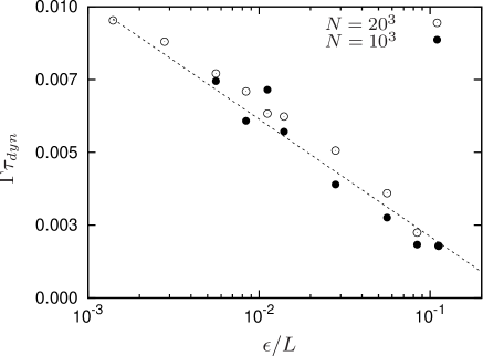
(c)

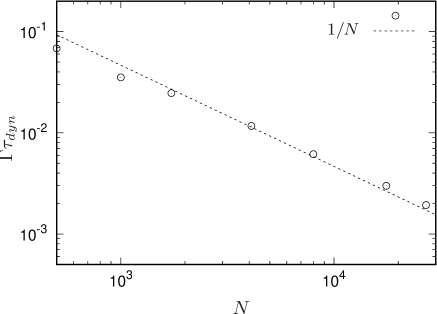
(d)

Figure 6: Measures of relaxation times for the case of gravity ($\gamma=1$): (a) Evolution of the indicator $\Delta(t)$ for chosen values of $\epsilon$ and fixed $N=8000$, i.e., in the set of simulations $\mathcal{C}(1;8000,\epsilon/L)$; (b) evolution of $\Delta(t)$ for the range of different $N$ simulated and $\epsilon=0.01$ i.e., the set of simulations $\mathcal{C}(1;N,0.01)$; (c) plot of $\Gamma\tau_{dyn}$ as a function of $\epsilon/L$ for both $N=8000$ and $N=1000$. In the latter case, following Eq. (49), the amplitude of the relaxation rate has been multiplied by a factor $8$ in order to collapse both the scalings on a single curve; the straight line is the theoretical scaling $\Gamma\tau_{dyn}\sim\epsilon^{-1}$; (d) plot of $\Gamma$ as a function of $N$ for fixed $\epsilon/L=0.01$.

Figs. 6a and 6b show the evolution of the collisional relaxation parameter $\Delta(t)$, defined in Eq.(54), as a function of time, for different values of $\epsilon$ and $N$. We estimate the relaxation rate as the slope of a linear fit to $\Delta(t)$ at short times. Inspecting Fig. 5a or 5b, we assume that the QSS has been reached at $t=10\tau_{dyn}$, and we take the reference time $t^{*}$ to evaluate the slope of $\Delta(t)$ as $t^{*}=20\tau_{dyn}$. We can estimate the value of $b_{0}$ using Eq. (13) by measuring the relative velocity from the simulation. This gives $b_{0}/L\approx 8.8\times 10^{-5}$. As this is considerably smaller even that the smallest softening used, we expect that the relaxation rate will scale as in Eq. (49) rather than Eq. (42). We show in Figs. 6c and 6d the measured scalings of the relaxation rate with $\epsilon$ and $N$ respectively. We observe that there is indeed very good agreement with the theoretical scaling of Eq. (49).

V Results for potentials with $\gamma\neq 1$

We now consider the case of power law interactions other than gravity. We consider first pair interactions which decrease more rapidly at large separations than the gravitational one, i.e., $\gamma>1$, and then the case $\gamma<1$.

V.1 Interactions decaying faster than gravity ($\gamma>1$)

We present results for two specific cases: $\gamma=5/4$ and $\gamma=3/2$. As discussed above we do not consider even larger values because, as predicted by the our analytical calculations, the two body collision rates indeed increase rapidly as $\gamma$ does, making it more and more difficult numerically to separate the associated time scale from the mean field one. Indeed from Eq.  (48) it follows that, at fixed $N$, the relaxation rate scales as $\epsilon^{-2\gamma}$.

Figs. 7a and 7b display results for the case $\gamma=5/4$, in a manner completely analogous to the case of gravity above. We observe a very similar behavior to that in the gravitational case: the curves of the total kinetic energy are superimposed at the early stage of evolution, and start to separate as time increases. Consistent with the interpretation of this drift as due to two body relaxation, we observe that it becomes slower for larger $N$ and larger $\epsilon$.

For our quantitative analysis of the collisional relaxation we choose the reference time $t^{*}=10\tau_{dyn}$, as the oscillations about the QSS are small by this time. For the case $\gamma=3/2$, for which we do not show the data (which is qualitatively very similar), we take $t^{*}=5\tau_{dyn}$. Fig. 7a show the time evolution, for $t>t^{*}$, of $\Delta(t)$, $N=8000$ and different values of the softening $\epsilon$. The velocity distribution at $t=2t^{*}$ is plotted in Fig. 7c, and the evolution of the parameters $\phi_{4}$ and $\phi_{6}$ as a function of time, shows that the system has a velocity distribution quite close to Gaussian, and apparently evolves progressively closer to such a distribution, as expected. Very similar behaviors are observed for the case $\gamma=3/2$. We do not plot the radial density profile, but it has a form which varies little with $\gamma$ and thus very similar to that plotted in Fig. 5e.

We estimate the relaxation rate in the same manner as we did above for the case of gravity, using the evolution of the indicator $\Delta(t)$ (which we do not plot). Estimating again the value of $b_{0}$ using Eq. (13), we obtain $b_{0}/L\approx 2.5\times 10^{-4}$ for $\gamma=5/4$, and $b_{0}/L\approx 7.3\times 10^{-4}$ for $\gamma=3/2$. As in the case of gravity, these are therefore much smaller than the minimal softening $\epsilon$ used, and we thus expect that the scaling of the relaxation rate should be given by Eq. (48).

Fig. 8a shows the measured relaxation rate for a range of softenings $\epsilon$ (for compact softening) at constant particle number $N=8000$, for both $\gamma=5/4$ and $\gamma=3/2$. Fig. 8b shows the scaling of the relaxation rate at varying $N$ and constant $\epsilon/L=0.01$. The error bars have been determined as the statistical error in the fit of $\Delta$, and are smaller than the size of the symbols. We observe that there is very good agreement between the scalings measured and the theoretical one (48). For the largest values of $\epsilon$ we observe a departure from the theoretical scaling. This is due to the finite size of the system (when $\epsilon$ is around one tenth of the size of the system, where the latter is estimated from the fall-off of the density profile).

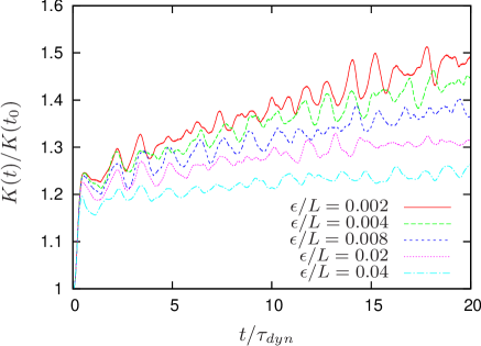
(a)

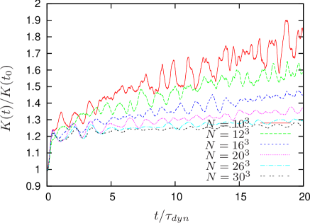
(b)

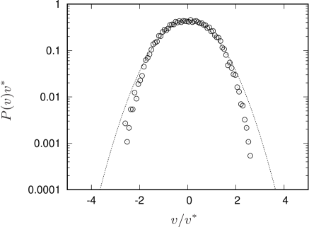
(c)

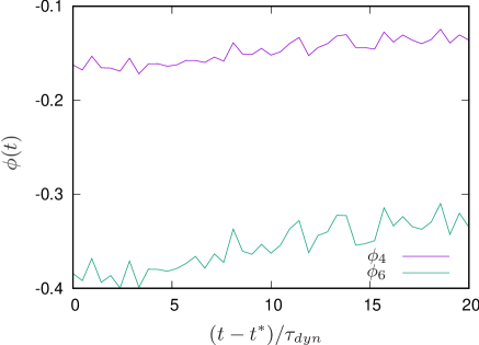
(d)

Figure 7: Results of simulations for the case $\gamma=5/4$: (a) Evolution of the normalized total kinetic energy for different values of $\epsilon$ at fixed $N=8000$, i.e., the set of simulations $\mathcal{C}(5/4;8000,\epsilon)$, (b) same quantity but for varying $N$ and fixed $\epsilon/L$, (c) velocity distribution for the simulation $\mathcal{C}(5/4;8000,0.002)$ at $t=10\tau_{dyn}$, and (d) evolution of $\phi_{4}$ and $\phi_{6}$ for the simulation $\mathcal{C}(5/4;8000,0.002)$.

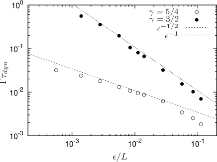
(a)

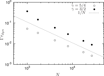
(b)

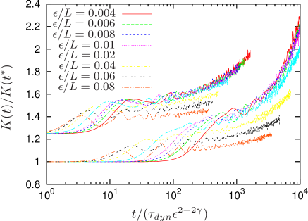
(c)

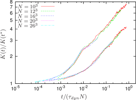
(d)

Figure 8: Tests of scaling of measured relaxation rates: (a) $\Gamma\tau_{dyn}$ as a function of $\epsilon$ (compact softening), for the cases $\gamma=5/4$ and $\gamma=3/2$ in simulations, and (b) as a function of $N$ for $\gamma=5/4$ and $\gamma=3/2$, (c) collapse plot at $N=20^{3}$ constant and varying $\epsilon$ for $\gamma=5/4$ (upper curves, all the curves have been multiplied by a factor of $1.25$) and $\gamma=3/2$ and (d) collapse plot at constant $\epsilon/L=0.1$ and varying $N$ for $\gamma=5/4$ (lower plot) and $\gamma=3/2$.

V.2 Relaxation at longer times

In the previous subsections we have considered collisional relaxation over time scales over which the parameters used to monitor evolution change by a small amount. In principle the predicted scalings should apply also on longer time scales, provided the scale introduced by the softening length is sufficiently small that it does not affect significantly the properties of the QSS.

Fig. 8c shows the normalized total kinetic energy for the case $\gamma=5/4$ (top curves) and $\gamma=3/2$ (bottom curves) for a constant particle number $N$ and a range of $\epsilon$. The time axis has been rescaled following the theoretical scaling (43). We observe a good superposition of the curves for the smaller values of $\epsilon$, while for softening approaching the size of the system the observed relaxation rate is suppressed compared to the theoretical prediction, just as for the shorter time relaxation (see Fig. 8a). Fig. 8d shows an analogous collapse plot but for a (small) constant $\epsilon$ and varying $N$, with the time axis now rescaled with $N$ following (43). We observe a very good matching between the different curves over the whole duration of the runs.

V.3 Results: case $\gamma<1$

In this case we have seen that the scaling of the relaxation rate is very simple: inversely proportional to $N$, and independent of the softening (cf. Eq. (47)). This behavior is a consequence of the fact that the dominant contribution comes from the largest impact factor, which we have assumed to scale with the system size. To test this prediction we have simulated the case $\gamma=1/2$. Fig. 9a shows the evolution of the normalized kinetic energy as function of time for a range of (compact) softenings $\epsilon$, while Fig. 9b shows the same quantity for a range of $N$ at fixed (small) $\epsilon$, as a function of a time variable linearly rescaled with $N$ in accordance with the the predicted scaling. We observe that the results are in excellent agreement with the theoretical predictions.

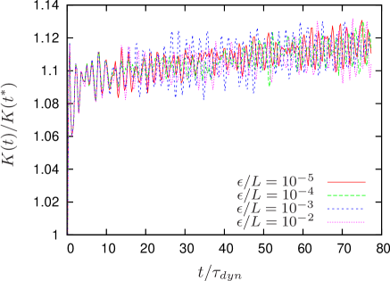
(a)

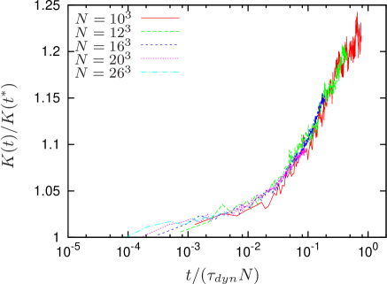
(b)

Figure 9: Evolution of the kinetic energy for systems with $\gamma=1/2$: (a) for a range of different values of $\epsilon$ at fixed $N=8000$, and (b) for a range of $N$ different number of particles at fixed $\epsilon$=0.0028 . In the latter plot the time variable has been rescaled with $N$ in line with the theoretically predicted scaling of Eq.

VI Tests of analytical predictions: beyond scaling

In the previous sections we have tested numerically the validity of the theoretical scaling relations derived in the first part of the paper. We now examine further how well the amplitudes of the measured relaxation rates match the predictions.

As we have discussed (see also Marcos (2013)), the approach we have adopted in deriving two body collision rates, following that used originally by Chandrasekhar for gravity, makes a number of very strong simplifying assumptions which make the calculation intrinsically inaccurate, notably: spatial homogeneity of the system and the assumption that all collisions take place at fixed relative velocity fixed by the global velocity dispersion. Further the “largest impact factor”, which we taken it to be given by the system size, is not in fact a precisely defined quantity and indeed it is often treated as a free parameter (see e.g. Meritt (2013) for a discussion in the context of the orbit-averaging technique). Other collisional effects which have been identified through the study of kinetic equations, such as orbit resonances and various collective effects (see e.g. Chavanis (2012b)), are also evidently not taken into account. Thus, even if incoherent two body scatterings are the dominant collisional process, we cannot expect the calculation method given to provide a precise prediction for the relaxation rates. Nevertheless the fact that the predicted scalings turn out to be in such good agreement with those observed, one would expect the quantitative discrepancies not to be too large.

VI.1 Effect of softening function

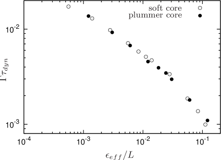
(a)

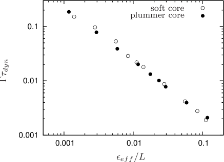
(b)

Figure 10: Measured relaxation rates as a function of $\epsilon_{eff}$ for the two different softening functions, for (a) $\gamma=5/4$ and (b) $\gamma=3/2$.

In subsections II.4 and III.3 we have discussed how the softening of the potential at small scales effects the predicted relaxation rate. The predicted modification depends, in general, not just on the value of the softening scale, but on the detailed form of the softened potential. We have noted, however, that for $\epsilon\gg b_{0}$, the effect of any such smoothing is an overall amplitude shift (cf. Fig. (4)). This allowed us to define, for any softening potential, a constant $\alpha$ giving an effective softening $\epsilon_{eff}=\alpha\epsilon$. The latter is the value of the softening of a reference softened potential which is sharply cut-off at $\epsilon_{eff}$, which gives the same predicted relaxation rate as the actual softened potential. The values of $\alpha$ for the two potentials (compact and Plummer) we have employed are given in Table 1.

Thus the theoretical calculations of the two body relaxation rates make a prediction about the relative amplitude of the relaxation rates for our two different smoothings, which we should expect to hold even if the prediction of the absolute amplitude of both is (expected to be) incorrect. Figs. 10a and 10b shows the relaxation rate measured in simulations with $N=8000$, as a function of the calculated $\epsilon_{eff}$ over a wide range. The superposition of the two curves is almost perfect, in line with the theoretical prediction.

VI.2 Detailed comparison of relaxation rates

We now compare directly the amplitudes of the predicted and measured relaxation rates. Tab. 3 shows, for the different values of $\gamma$ we have simulated, the results of this comparison. The second column gives the numerical value of $b_{0}\approx\left(g/(m\langle v^{2}\rangle)\right)^{1/\gamma}$, where $\langle v^{2}\rangle$ is the velocity dispersion measured at $t=20\tau_{dyn}$ in the simulations (we have used that $\langle V^{2}\rangle\simeq 2\langle v^{2}\rangle$). Using this value for $b_{0}$, and taking $R=0.3$ for the system size (cf. Figs. 5e and 5f), we have calculated numerically the predicted $\Gamma\tau_{\rm dyn}$ shown in the third column (“Theory”) using Eq. (23). The fourth column (“Numerics”) gives the value of $\Gamma\tau_{\rm dyn}$ estimated in our simulations from the short time evolution of the normalized total kinetic energy $K(t)/K(t_{0})$ as described in Sect. IV.2. Comparing the last columns we find that, despite the many crude approximations performed in the derivation of the relaxation rate we obtain, as we have seen, not only the right scaling with the relevant parameters, but also a relatively good quantitative agreement for the amplitudes for all the cases simulated, with an overall discrepancy in the normalization varying between a factor one and eight. Moreover, we observe that, as $\gamma$ increases, the agreement is better. This is compatible with the idea that as the interaction becomes less long range, the resonances between particles with different frequencies become less important and a local approximation better and better (see e.g. Heyvaerts (2010)).

$\gamma$	$b_{0}\approx(g/(2m\langle V^{2}\rangle))^{1/\gamma}$	Theory	Numerics
1/2	$9.2\times 10^{-8}$	$7.4\times 10^{-3}$	$4.6\times 10^{-4}$
3/4	$8.4\times 10^{-6}$	$1.4\times 10^{-2}$	$1.1\times 10^{-3}$
1	$8.8\times 10^{-5}$	$0.016$	$4.6\times 10^{-3}$
5/4	$3.7\times 10^{-4}$	$0.059$	$0.023$
3/2	$8.7\times 10^{-4}$	$0.017$	$0.24$

Table 3: Comparison of the theoretical and measured relaxation rates in the simulations. The second column corresponds to an estimation of $b_{0}$, the third one to the estimation of $\langle|\Delta{\mathbf{V}}^{2}|\rangle/|V^{2}|$ using Eq. (23) and the fourth one the relaxation time measured in the simulations (see text).

VI.3 Constraining the maximum impact factor

Going back to the original derivation of the two body relaxation rate by Chandrasekhar there has been a debate about the correct choice of the maximum impact parameter. In section II.1 we have argued that it should be assumed to be of the order of the size of the system, and we have obtained our results making this hypothesis.

For the case $\gamma\leq(d-1)/2$, which is dominated by the largest impact factors, we can in principle test this hypothesis. If, instead of Eq. (41), we fix an arbitrary maximum parameter $b_{max}$, it is straightforward to show that we obtain

$$\Gamma\tau_{dyn}=\tilde{C}N^{-1}\left(\frac{R}{b_{max}}\right)^{2\gamma-d+1},$$ (59)

where $\tilde{C}$ is a numerical coefficient (depending only on $\gamma$ and $d$). If we now assume that $b_{max}\sim RN^{-\alpha}$ we obtain

$$\Gamma\tau_{dyn}\sim N^{\beta},$$ (60)

where $\beta=\alpha(2\gamma-d+1)-1$. The case $\alpha=0$ corresponds to the assumption we have made up to now, and the result (41). The case $\alpha=1/d$ corresponds, on the other hand, to the assumption that $b_{max}$ scales in proportion to the inter-particle distance (as originally assumed by Chandrasekhar Chandrasekhar (1942)). Now we have seen in section V that the scaling of the relaxation rate for the simulated cases $\gamma=1/2$ and $\gamma=3/4$ are $\Gamma\tau_{dyn}\sim N^{-1}$, which are in agreement with $\beta=0$ and hence $b_{max}\sim R$.

In the specific case $\gamma=(d-1)/2$, i.e. gravity in $d=3$, it is in fact possible to quantify the maximum impact factor rather than just its scaling. Instead of Eq. (49) (replacing $\epsilon$ by $\epsilon_{eff}$ following the discussion in Sect. III.3) we have

$$\Gamma\tau_{dyn}=\tilde{D}N^{-1}\ln\left(\frac{b_{max}}{\epsilon_{eff}}\right),$$ (61)

where $\tilde{D}$ is a (calculable) numerical coefficient. Using the simulations presented in Sect. IV, we can fit very well the relaxation rate with

$$\Gamma\tau_{dyn}=\ln\left(\frac{L}{3\epsilon_{eff}}\right)\frac{7.2}{N}.$$ (62)

Comparing these last two equations, we have that $\alpha\approx 0$, and, further, that $b_{max}\approx L/3\approx R/3$. This size corresponds with the sharp fall-off of the density profile shown in the inset of Fig. 5f. To check that $b_{max}$ does not depend on $N$, we did another set of simulations with the same parameters but $N=1000$ particles. From these we obtained the scaling of the relaxation rate as a function of $\epsilon$ plotted in Fig. 6c, in which, according to Eq. (49), the relaxation rate has been multiplied by a factor of eight. We thus obtain very good agreement with the predicted scaling. Our findings confirm therefore the results of Farouki & Salpeter Farouki and Salpeter (1982, 1994), who found that the maximum impact parameter should be taken of order of the size of the system.

VII Conclusion

In this paper, we have studied collisional relaxation in systems of particles interacting with a power-law potential $v(r\to\infty)\sim 1/r^{\gamma}$ (1), introducing a regularization of the singularity in the force as $r\rightarrow 0$ when necessary. In our analytical calculations we have generalized the “Chandrasekhar approach” in the case of gravity to such potentials. We have also included the contribution of hard collisions rather than just weak collisions, in which the mean field trajectories of the particles are weakly perturbed, which is the approximation usually found in the literature, see e.g. Chavanis (2012b). We have found that the collisional dynamics is dominated by

• weak collisions, if $\gamma<(d-1)/2$, and

• hard collisions, if $\gamma>(d-1)/2$,

while the case $\gamma=(d-1)/2$, which corresponds to gravity in $d=3$, is at the threshold. Moreover we considered the large $N$, mean field (or Vlasov) limit scaling of the two body relaxation rate, assuming the considered particle system to be in viral equilibrium. In absence of force regularization (other than an infinitesimal one assumed implicitly to make two body collisions defined for $\gamma>2$), we found that this rate, expressed in units of the characteristic time for mean-field dynamics $\tau_{dyn}$, vanishes in the large $N$ for $\gamma<d-1$, and diverges in this limit for $\gamma>d-1$. This means that only in the former case does the mean-field limit of the dynamics exist for a virialized system; in the latter case it does not because the collisional relaxation completely dominates the mean field dynamics. Only in the former case, therefore, can a QSS be expected to exist on a physically relevant time scale. This leads to the following dynamical classification of interactions:

1. Power-law interactions is dynamically long-range if $\tau_{dyn}\ll\tau_{coll}$ for a sufficiently large number of particles, and in particular $\lim_{N\to\infty}\Gamma\tau_{dyn}=0$, which occurs for $\gamma<d-1$.

2. The interaction is dynamically short range if $\tau_{dyn}\gg\tau_{coll}$ for a sufficiently large number of particles, and in particular $\lim_{N\to\infty}\Gamma\tau_{dyn}=\infty$, which occurs for $\gamma<d-1$.

This classification was proposed initially Gabrielli et al. (2010b) on the basis of a formal analysis of convergence properties of the force on a particle in the thermodynamic limit, and subsequently in Gabrielli et al. (2010a) on the basis of the analysis detailed here. It has also been justified using different analytical approaches to the full kinetic theory of such systems Chavanis (2013); Gabrielli et al. (2014). As noted in the introduction, this classification differs from the usual one used to distinguish long range from short range interactions, according to the thermal equilibrium of the system, in which the important feature is the integrability of the potential. There is therefore a range of $\gamma$, $d-1<\gamma<d$, in which the interaction is dynamically short range, but long-range according to its thermal equilibrium properties. In this case, if the number of particles is sufficiently large, there will be no QSS (as in short range systems), but the thermal equilibrium state will present the typical features of a long-range system, i.e., spatial inhomogeneity, inequivalence of ensembles etc..

We have also generalized these scalings when the inter–particle potential is regularized (“softened”) at small scales. With this regularization the case $\gamma\geq 2$ (in which the potential barrier cannot prevent the particles to collide for pure power–law potentials) becomes well defined. In this case, the relaxation rate depends on the value of the softening length $\epsilon$ for interactions in which small impact factors play a predominant role, i.e., $\gamma\leq(d-1)/2$.

We have presented, for $d=3$, detailed numerical results which support our theoretical findings. We have confirmed previous results in the literature for the gravitational case $\gamma=1$, notably for the scaling relations satisfied by the relaxation rate as function of the softening $\epsilon$ and the number of particles $N$. Furthermore, using the scaling of the relaxation rate with $\epsilon$, we have found very strong numerical evidence that the maximum impact parameter is related with the size of the system and not microscopic scales such as the inter-particle distance. We have simulated also dynamically long-range cases $\gamma=5/4$ and $\gamma=3/2$, in which the collisional relaxation is dominated by collisions around the minimum impact parameter, obtaining again very good agreement with the theoretical scalings. For dynamically long-range systems dominated in our calculations by collisions with the largest impact parameter, we have found find, as predicted, that a softening in the potential does not affect the relaxation rate.

The natural extension of this work is the numerical study of collisional relaxation allowing strong collisions, in order to check the scalings of this regime derived in this paper. For such study, it is necessary to develop very refined integration schemes in order to integrate properly such collisions. Another interesting perspective is to study the problem with a more rigorous approach using the angle-action variables (with probably also many approximations because it is a very complicated formalism) in order to describe more precisely the relaxation dynamics, and in particular study more precisely the validity of the Chandrasekhar approximation as a function of the range of the interaction $\gamma$.

Appendix A An alternative derivation of the change in perpendicular velocity due to a collision

It is interesting to derive Eq. (18a) simpler method which can give more physical insight. We can compute the change in perpendicular velocity integrating the perpendicular component of the force for all the duration of the collision, assuming that the relative trajectories is unperturbed with constant relative velocity $V$:

$$F_{\perp}=\frac{\gamma g}{b^{\gamma+1}}\left[1+\left(\frac{Vt}{b}\right)^{2}\right]^{-(\frac{\gamma}{2}+1)},$$ (63)

The change in the perpendicular component of the velocity in a time $2t_{c}$ is thus

$$|\Delta{\mathbf{V}}_{\perp}| = \frac{\gamma g}{mb^{\gamma+1}}\int_{-t_{c}}^{t_{c}}dt\left[1+\left(\frac{Vt}{b}\right)^{2}\right]^{-(\frac{\gamma}{2}+1)}$$ (64)

$$= \frac{\gamma g}{mb^{\gamma}V}\int_{\frac{Vt_{c}}{b}}^{-\frac{Vt_{c}}{b}}ds(1+s^{2})^{-(\frac{\gamma}{2}+1)}$$ (65)

$$\simeq \gamma\left(\frac{b_{0}}{b}\right)^{\gamma}\int_{-\infty}^{\infty}ds(1+s^{2})^{-(\frac{\gamma}{2}+1)};$$ (66)

Taking the limit $t_{c}\to\infty$ and performing the integral we obtain exactly (18a).

Appendix B Exact form of the potential with a soft core

The potential $v(r,\epsilon)$ is, for $r\geq\epsilon$, exactly

$$v(r\geq\epsilon,\epsilon)=\frac{g}{r^{\gamma}}.$$ (67)

We define $u=r/\epsilon$. For $u<1$ we use the following form of the potential for soft core softenings:

• $\gamma=1/2$:

  $$v(u,1)\epsilon^{1/2}=15.75u^{2}-22.5u^{3}+8.75u^{4},$$ (68)

• $\gamma=3/4$:

  $$v(u,1)\epsilon^{3/4}=11.875u^{2}-17.4167u^{3}+6.875u^{4},$$ (69)

• $\gamma=1$:

  $$v(u,1)\epsilon=10u^{2}-15u^{3}+6u^{4},$$ (70)

• $\gamma=5/4$:

  $$v(u,1)\epsilon^{5/4}=8.925u^{2}-13.65u^{3}+5.525u^{4},$$ (71)

• $\gamma=3/2$:

  $$v(u,1)\epsilon^{3/2}=8.25u^{2}-12.8333333u^{3}+5.25u^{4}.$$ (72)

  

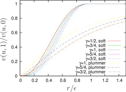
  Figure 11: Softened potentials used in the paper normalized to the unsoftened one.

References

- Binney and Tremaine (2008) J. Binney and S. Tremaine, Galactic Dynamics (Princeton University Press, 2008).
- Chavanis (2002) P. H. Chavanis, Dynamics and Thermodynamics of Systems with Long-Range Interactions (Springer, New York, 2002).
- Chalony et al. (2013) M. Chalony, J. Barré, B. Marcos, A. Olivetti, and D. Wilkowski, Phys. Rev. A 87, 013401 (2013).
- Campa et al. (2009) A. Campa, T. Dauxois, and S. Ruffo, Phys. Reports 480, 57 (2009).
- Ispolatov and Cohen (2001) I. Ispolatov and E. G. D. Cohen, Phys. Rev E64, 056103 (2001).
- Chavanis (2013) P.-H. Chavanis, European Physical Journal Plus 128, 128 (2013).
- Kastner (2011) M. Kastner, Phys. Rev. Lett. 106, 130601 (2011).
- Cevolani et al. (2016) L. Cevolani, G. Carleo, and L. Sanchez-Palencia, New J. Phys. 18, 093002 (2016).
- Chandrasekhar (1942) S. Chandrasekhar, Principles of stellar dynamics (University of Chicago Press, 1942).
- Yamaguchi et al. (2004) Y. Y. Yamaguchi, J. Barré, F. Bouchet, T. Dauxois, and S. Ruffo, Physica A 337, 36 (2004).
- Joyce and Worrakitpoonpon (2010) M. Joyce and T. Worrakitpoonpon, Journal of Statistical Mechanics: Theory and Experiment 10, 12 (2010).
- Teles et al. (2010) T. N. Teles, Y. Levin, R. Pakter, and F. B. Rizzato, Journal of Statistical Mechanics: Theory and Experiment 5, 7 (2010).
- Marcos (2013) B. Marcos, Phys. Rev. E 88, 032112 (2013).
- Levin et al. (2014) Y. Levin, R. Pakter, F. B. Rizzato, T. N. Teles, and F. P. d. C. Benetti, Phys. Reports 535, 1 (2014).
- Chavanis (2012a) P.-H. Chavanis, Astron. Astrophys. 556 A93 (2013).
- Braun and Hepp (1977) W. Braun and K. Hepp, Comm. Math. Phys. 56, 101 (1977).
- Spohn (1991) H. Spohn, Large Scale Dynamics of Interacting Particles (Springer-Verlag, 1991).
- Hauray and Jabin (2007) M. Hauray and P. E. Jabin, Arch. Rational Mech. Anal. 183, 489 (2007).
- Boers and Pickl (2013) N. Boers and P. Pickl, J. Stat. Phys. (2016), 164:1.
- Lazarovici and Pickl (2015) D. Lazarovici and P. Pickl, ArXiv e-prints (2015), eprint 1502.04608.
- Weinberg (1993) M. D. Weinberg, Astrophys. J. 410, 543 (1993).
- Heyvaerts (2010) J. Heyvaerts, Mon. Not. R. Astr. Soc. 407, 355 (2010).
- Chavanis (2012b) P.-H. Chavanis, Physica A Statistical Mechanics and its Applications 391, 3680 (2012b).
- Fouvry et al. (2015a) J. B. Fouvry, C. Pichon, J. Magorrian, and P. H. Chavanis, A&A 584, A129 (2015a).
- Fouvry et al. (2015b) J. B. Fouvry, C. Pichon, and P. H. Chavanis, A&A 581, A139 (2015b).
- Fouvry and Pichon (2015) J.-B. Fouvry and C. Pichon, MNRAS 449, 1982 (2015).
- Fouvry et al. (2016a) J.-B. Fouvry, C. Pichon, and J. Magorrian, ArXiv e-prints (2016a), eprint 1606.05501.
- Fouvry et al. (2016b) J.-B. Fouvry, C. Pichon, and P.-H. Chavanis, ArXiv e-prints (2016b), eprint 1605.03384.
- Benetti and Marcos (2016) F. P. C. Benetti and B. Marcos, ArXiv e-prints (2016), eprint 1610.06966.
- Gabrielli et al. (2010a) A. Gabrielli, M. Joyce, and B. Marcos, Physical Review Letters 105, 210602 (2010a).
- Gabrielli et al. (2010b) A. Gabrielli, M. Joyce, B. Marcos, and F. Sicard, Journal of Statistical Physics 141, 970 (2010b).
- Gabrielli et al. (2014) A. Gabrielli, M. Joyce, and J. Morand, Phys. Rev. E 90, 062910 (2014).
- Chandrasekhar (1943) S. Chandrasekhar, Astrophys. J. 97, 255 (1943).
- Hénon (1958) M. Hénon, Annales d’Astrophysique 21, 186 (1958).
- Chavanis (2010) P.-H. Chavanis, Journal of Statistical Mechanics: Theory and Experiment 5, 19 (2010).
- Diemand et al. (2004) J. Diemand, B. Moore, J. Stadel, and S. Kazantzidis, Mon. Not. Roy. Astron. Soc. 348, 977 (2004).
- Farouki and Salpeter (1982) R. T. Farouki and E. E. Salpeter, Astrophys. J. 253, 512 (1982).
- Smith (1992) H. Smith, Jr., Astrophys. J. 398, 519 (1992).
- Farouki and Salpeter (1994) R. T. Farouki and E. E. Salpeter, Astrophys. J. 427, 676 (1994).
- Theis (1998) C. Theis, Astron. Astrophys. 330, 1180 (1998).
- Gabrielli et al. (2010c) A. Gabrielli, M. Joyce, and B. Marcos, Physical Review Letters 105, 210602 (2010c).
- Landau and Lifshitz (1976) L. D. Landau and E. M. Lifshitz, Mechanics (Butterworth-Heinemann, 1976).
- Chiron and Marcos (2015) D. Chiron and B. Marcos (2015).
- Balescu (1997) R. Balescu, Statistical Mechanics. Matter out of equilibrium (Imperial College Press, 1997).
- Di Cintio et al. (2013) P. Di Cintio, L. Ciotti, and C. Nipoti, Mon. Not. R. Astron. Soc. 431, 3177 (2013).
- Di Cintio et al. (2015) P. Di Cintio, L. Ciotti, and C. Nipoti, Journal of Plasma Physics 81, 495810504 (2015).
- Springel (2005) V. Springel, Mon. Not. R. Astron. Soc 364, 1105 (2005).
- White (1978) S. D. M. White, MNRAS 184, 185 (1978).
- Meritt (2013) D. Meritt, Dynamics and Evolution of Galactic Nuclei (Princeton University Press, 2013).