Ly$\alpha$ profile, dust, and prediction of Ly$\alpha$ escape fraction in Green Pea Galaxies

Abstract

We studied Lyman-$\alpha$ (Ly$\alpha$) escape in a statistical sample of 43 Green Peas with HST/COS Ly$\alpha$ spectra. Green Peas are nearby star-forming galaxies with strong [OIII]$\lambda$5007 emission lines. Our sample is four times larger than the previous sample and covers a much more complete range of Green Pea properties. We found that about 2/3 of Green Peas are strong Ly$\alpha$ line emitters with rest-frame Ly$\alpha$ equivalent width $>20$ Å. The Ly$\alpha$ profiles of Green Peas are diverse. The Ly$\alpha$ escape fraction, defined as the ratio of observed Ly$\alpha$ flux to intrinsic Ly$\alpha$ flux, shows anti-correlations with a few Ly$\alpha$ kinematic features – both the blue peak and red peak velocities, the peak separations, and FWHM of the red portion of the Ly$\alpha$ profile. Using properties measured from SDSS optical spectra, we found many correlations – Ly$\alpha$ escape fraction generally increases at lower dust reddening, lower metallicity, lower stellar mass, and higher [OIII]/[OII] ratio. We fit their Ly$\alpha$ profiles with the HI shell radiative transfer model and found Ly$\alpha$ escape fraction anti-correlates with the best-fit $N_{HI}$. Finally, we fit an empirical linear relation to predict $f^{Ly\alpha}_{esc}$ from the dust extinction and Ly$\alpha$ red peak velocity. The standard deviation of this relation is about 0.3 dex. This relation can be used to isolate the effect of IGM scatterings from Ly$\alpha$ escape and to probe the IGM optical depth along the line of sight of each $z>7$ Ly$\alpha$ emission line galaxy in the JWST era.

1. Introduction

In young star forming galaxies, Lyman continuum (LyC) photons from hot stars ionize the surrounding hydrogen gas, and Ly$\alpha$ photons come from the recombination of hydrogen gas. The Ly$\alpha$ emission line is a powerful tool in discovering and studying high redshift galaxies. Thousands of high redshift Ly$\alpha$ emission line galaxies (LAE) have been found in the last two decades (e.g. Dey et al. 1998; Hu et al. 1998; Rhoads et al. 2000; Ouchi et al. 2003; Gawiser et al. 2006; Wang et al. 2009; Kashikawa et al. 2011; Erb et al. 2014; Matthee et al. 2014; Zheng et al. 2016). These high redshift LAEs generally have small size, low stellar mass, low dust extinction, low metallicity, young age, and high specific star formation rate (sSFR) (e.g. Malhotra 2012; Bond et al. 2010; Gawiser et al. 2007; Pirzkal et al. 2007; Finkelstein et al. 2008). At $2\mathrel{\hbox{\hbox to0.0pt{\hbox{\lower 4.0pt\hbox{$\sim$}}\hss}\hbox{$<$}}}z\mathrel{\hbox{\hbox to0.0pt{\hbox{\lower 4.0pt\hbox{$\sim$}}\hss}\hbox{$<$}}}6$, these LAEs are an important population of star-forming galaxies, and they constitute an increasing fraction of Lyman break galaxies across that range, reaching $\sim 60\%$ of Lyman break galaxies (LBGs) at redshift $z\sim$6 (Stark et al. 2011).

A current frontier is searching for LAEs in the epoch of Cosmic Reionization. As Ly$\alpha$ photons propagate from a LAE to the observer, they pass through the intergalactic medium (IGM) and will be scattered away from the line of sight by HI in IGM. So Ly$\alpha$ line can be used to probe reionization of IGM (e.g. Malhotra & Rhoads 2004; Treu et al. 2012; Pentericci et al. 2014; Tilvi et al. 2014; Matthee et al. 2015; Santos et al. 2016). These Ly$\alpha$ based methods can effectively probe HI fraction in the later half of reionization. One major goal of JWST is to observe the Ly$\alpha$ and rest-frame optical lines spectra of $z>7$ galaxies and probe reionization with Ly$\alpha$ lines. However, the challenge is to isolate the impact of IGM from other effects that may diminish Ly$\alpha$. The Ly$\alpha$ photons have to escape out of the galaxies before passing through the IGM and being observed, i.e. $(Observed\ Ly\alpha)=(Intrinsic\ Ly\alpha)\times\ (Ly\alpha\ escape\ fraction)\times(IGM\ Transmission)$. The Ly$\alpha$ escape fraction describes how many Ly$\alpha$ photons escape out of both interstellar medium (ISM) and circum-galactic medium (CGM) of a LAE. Thus, to use Ly$\alpha$ reionization tests, we have to understand Ly$\alpha$ escape and predict Ly$\alpha$ escape fraction from other properties.

Ly$\alpha$ escape is also related to the LyC escape process. A large fraction ( 9/12) of known LyC leakers are LAEs (Leitet et al. 2013; Borthakur et al. 2014; Izotov et al. 2016; Leitherer et al. 2016; de Barros et al. 2016; Shapley et al. 2016). LAEs at the reionization epoch may be major contributors of ionizing photons. Ly$\alpha$ line profiles may be used as a tool for detecting LyC leakers (Verhamme et al. 2015; Alexandroff et al. 2015; Dijkstra et al. 2016). Understanding Ly$\alpha$ escape is very useful for the study of LyC escape.

As Ly$\alpha$ is a resonance line, it has a high cross-section for HI scattering. The emergent Ly$\alpha$ emission has a complicatedly dependence on the amount of dust, the HI gas column density ($N_{HI}$), the kinematics of HI gas, and the geometric distribution of HI gas and dust (e.g. Neufeld 1990; Charlot & Fall 1993; Ahn et al. 2001; Verhamme et al. 2006; Dijkstra et al. 2006; Laursen et al. 2013). The scattering of Ly$\alpha$ photons can significantly modify the Ly$\alpha$ line profile. LAEs usually show asymmetric or a double-peaked Ly$\alpha$ emission line profiles (e.g. Rhoads et al 2003; Kashikawa et al. 2011; Erb et al. 2014). Therefore the Ly$\alpha$ line profile carries a lot of information about the resonant scatterings and can be used to probe the HI gas properties.

To study Ly$\alpha$ escape, it is ideal to have a large sample of LAEs and measure high quality Ly$\alpha$ line spectrum, many optical emission lines, HI gas properties, and multiple other galactic properties. So we can test what properties make Ly$\alpha$ escape, and finally predict Ly$\alpha$ escape fraction from those properties. At high redshift, however, absorption by the intergalactic Ly$\alpha$ forest prevents reliable measurements of the blue portion of Ly$\alpha$ emission lines. Other crucial observations are also impractical, both because high-$z$ LAEs are faint, and because some features (notably rest-optical emission lines) are redshifted to $\lambda_{obs}>2.4{\mu}m$, where presently available instruments lack sensitivity. Therefore many studies seek to solve the Ly$\alpha$ escape problem by observing low-$z$ galaxies with similar properties to high-$z$ LAEs (e.g. Giavalisco et al. 1996; Kunth et al. 1998; Mas-Hesse et al. 2003; Deharveng et al. 2008; Finkelstein et al. 2009; Atek et al. 2009; Leitherer et al. 2011; Heckman et al. 2011; Cowie et al. 2011; Wofford et al. 2013; Hayes et al. 2005, 2014; Ostlin et al. 2014; Rivera-Thorsen et al. 2015). However, low-$z$ LAEs are rare and many nearby Ly$\alpha$ emission line galaxies are older and more evolved galaxies than typical high-$z$ LAEs and may be a different population of Ly$\alpha$ emitters. Perhaps the most relevant nearby analogs of high-$z$ LAEs are Green Pea galaxies (Jaskot & Oey 2014; Henry et al. 2015; Yang et al. 2016a, hereafter Paper I).

Green Pea galaxies were discovered in the citizen science project Galaxy Zoo, in which public volunteers morphologically classified millions of galaxies from the Sloan Digital Sky Survey (SDSS). Green Peas are compact galaxies that are unresolved in SDSS images. The green color is because the [OIII] doublet dominates the flux of SDSS $r$-band which is mapped to the green channel in the SDSS’s false-color gri-band images (Lupton et al. 2004). They generally have small stellar masses ($\sim 10^{8-10}M_{\odot}$), low metallicities for their stellar masses, high specific star formation rates (sSFR), and large [OIII]$\lambda$5007/[OII]$\lambda$3727 (hereafter [OIII]/[OII]) ratio (Cardamone et al. 2009; Amorin et al. 2010; Izotov et al. 2011). The UV spectra of 17 Green Peas generally show strong Ly$\alpha$ emission lines (Paper I; Jaskot & Oey 2014; Henry et al. 2015; Izotov et al. 2016; Verhamme et al. 2016). These studies have explored the relation of $f^{Ly\alpha}_{esc}$ and dust, metallicity, Ly$\alpha$ profiles, and metal absorption lines with small samples of Green Peas. Besides the small sample size, the previous samples of Green Peas tend to be lower metallicity and lower dust extinction than the whole Green Pea sample. In our HST program, we observed an additional 20 Green Peas in order to have a statistical sample that spans a range of galaxy properties such as metallicity, dust extinction, and star-formation rate (SFR).

In this paper, we use HST/COS Ly$\alpha$ spectra of Green Peas to study the mechanism of Ly$\alpha$ escape. In Section 2, we show the sample and observations. In Section 3, we describe the measurement and properties of Ly$\alpha$ equivalent width and escape fraction. In Section 4, we show the relation between Ly$\alpha$ escape and Ly$\alpha$ kinematic features. In Section 5, we show the relation between Ly$\alpha$ escape and dust extinction, metallicity, stellar mass, morphology, and [OIII]/[OII] ratio. In Section 6, we fit the Ly$\alpha$ profiles with radiative transfer model. In Section 7, we show an empirical relation to predict Ly$\alpha$ escape fraction and discuss its applications on probing reionization.

2. Sample and Observations

2.1. The Sample

Since the strong [OIII]$\lambda$5007 line makes Green Pea galaxies have special optical broadband colors, we can select a few thousand Green Pea candidates from the SDSS imaging survey (Yang et al. 2016 in-prep). In SDSS DR7, a sample of 251 Green Peas were observed as serendipitous spectroscopic targets (Cardamone et al. 2009). A subset of 66 Green Peas have sufficient signal to noise ratio (S/N) in both continuum and emission lines (H$\alpha$, H$\beta$, and [OIII]$\lambda$5007) to study galactic properties such as SFR, stellar mass, and metallicity (Cardamone et al. 2009; Izotov et al. 2011). Galaxies with an active galaxies nucleus (AGN) (diagnosed by their broad Balmer emission lines or H$\alpha$/[NII] vs. [OIII]/H$\beta$ diagram) are excluded. In Paper I, we matched these 66 Green Peas with the COS archive and studied Ly$\alpha$ escape in a sample of 12 Green Peas with COS UV spectra. Compared to the larger Green Pea sample, these 12 Green Peas tend to be lower metallicity and lower dust extinction (figure 1). To address the bias and expand the sample size, we took Ly$\alpha$ spectra of 20 additional Green Peas (PI S. Malhotra, GO 14201). These 20 galaxies were selected based on their metallicity and H$\alpha$/H$\beta$ values to supplement the previous sample, so that the total sample can cover the whole range of metallicity and dust extinction of the parent sample. We use figure 1 to do the selection – first draw grids (shown in figure 1), then pick one or two sources in each grid cell. Note that (a) empty cells are not used and (b) the non-empty cells are not covered perfectly because in the proposal we used gas metallicities measured in Izotov et al. (2011) which are slightly different from the metallicities shown in figure 1. After the selection, we compared the total sample with the parent sample to make sure there is no obvious biases.

We also supplement this sample with 11 additional Green Peas from published literature. In total, we have 43 Green Peas from six HST programs – 20 galaxies from GO 14201 (PI S. Malhotra), 9 galaxies from GO 12928 (PI A. Henry; Henry et al. 2015), 7 galaxies from GO 11727 and GO 13017 (PI T. Heckman; Heckman et al. 2011; Alexandroff et al. 2015), 2 galaxies from GO 13293 (PI A. Jaskot; Jaskot et al. 2014), and 5 galaxies from GO 13744 (PI T. Thuan; Izotov et al. 2016). The 7 galaxies in T. Heckman’s program were originally selected as nearby Lyman-break analogs by their high FUV luminosity, high UV flux, and compact size. These 7 galaxies can also be classified as Green Peas by their compact sizes in SDSS images and strong [OIII]$\lambda$5007 emission lines in SDSS spectra. Their sizes and [OIII]$\lambda$5007 equivalent width are similar to the Green Peas in Cardamone et al. (2009). We don’t find any obvious bias by including the Lyman-break analogs in the analysis. The 7 Green Peas in A. Jaskot’s program and T. Thuan’s program were selected as LyC leakers by their extreme [OIII]/[OII] ratios. In figure 1, we show the above samples on the metallicity and dust extinction (H$\alpha$/H$\beta$ ratio) diagram. We can see the current sample is a representative Green Pea sample.

2.2. Properties from SDSS Spectra

From SDSS optical spectra of Green Peas, we get many galactic properties. We use the SDSS pipeline measurements of their H$\alpha$, H$\beta$, [OIII]$\lambda$5007, and [OII]$\lambda$3727 emission line fluxes and line width. We correct the measured H$\alpha$ and H$\beta$ fluxes for Milky Way extinction using the attenuation of Schlafly & Finkbeiner (2011) (obtained from the NASA/IPAC Galactic Dust Reddening and Extinction tool) and the Fitzpatrick (1999) extinction law. Then we calculate E(B-V) assuming the Calzetti et al. (2000) extinction law and an intrinsic H$\alpha$/H$\beta$ ratio of 2.86 (if H$\alpha$/H$\beta$$<2.86$, we set E(B-V)=0), and correct the observed emission line fluxes for dust extinction. We use the stellar mass measured from SDSS spectra by Izotov et al. (2011) for 37 galaxies and the stellar mass in MPA-JHU SDSS catalog for the other 6 galaxies (all are Lyman-break analogs). Note that the methods used in Izotov et al. (2011) and MPA-JHU are different. The masses here should be treated as very rough estimates because it is very hard to get the masses of the underlying old population for these young starburst galaxies. To measure the metallicity using $T_{e}$ method, we measure the [OIII]$\lambda$4363 line flux in SDSS spectra by fitting a Gaussian function to the continuum subtracted [OIII]$\lambda$4363 line spectra. Then we calculate the metallicity using [OIII]$\lambda$4363, [OIII]$\lambda$5007, and [OII]$\lambda$3727 line fluxes following the $T_{e}$ method described in Izotov et al. (2006) and Ly et al. (2014). We convert the extinction corrected H$\alpha$ luminosity to SFR using the formula $SFR(M_{\odot}/yr)=L_{H\alpha}(erg/s)\times 10^{-41.27}$ (Kennicutt & Evans 2012). The dust extinction, mass, metallicity, SFR, and emission lines properties of this sample are shown in Table 1 and Table 2.

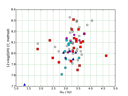
Figure 1.— The metallicity and dust extinction (H$\alpha$/H$\beta$ ratio) diagram of our Green Pea sample. Red squares shows the 20 galaxies with new HST observations (GO 14201, PI S. Malhotra). The other samples include 9 Green Pea galaxies with low dust extinction (cyan circle, Paper I; Henry et al. 2015), 7 Lyman-break analog galaxies (magenta pentagon, Heckman et al. 2011; Alexandroff et al. 2015), 2 Lyman-continuum leaker candidates (blue star, Jaskot et al. 2014), and 5 confirmed Lyman-continuum leakers (blue triangle, two blue triangles overlap; Izotov et al. 2016). The black hollow circles show the other galaxies without HST UV spectra in the sample of 66 Green Peas. Note that a few sources have very small Ha/Hb values. The reasons are not yet well understood, but could be 1) poor flat-field calibration or sky subtraction, 2) different gas conditions from the case-B assumption.

2.3. HST/COS Observation

In our program GO14201, we used HST/COS to observe 20 Green Peas with one orbit per target. First, the targets were imaged in the COS acquisition mode ACQ/IMAGE with MIRRORA, from which we got high resolution near-UV (NUV) images. The targets were centered accurately (error $\sim$ 0.05^′′) in the 2.5^′′ diameter Primary Science Aperture. Then the spectra were taken with grating G160M to cover rest-frame wavelength ranges about $1100-1400$ Å. The other archival Green Peas in our sample were also observed in the same COS acquisition mode ACQ/IMAGE with MIRRORA, and their spectra were taken with grating G130M and/or G160M. The NUV acquisition images of this sample are shown in figure 2.

The spectral resolution of the above observation is about FWHM$\sim$20 km s^-1 for a point source (James et al. 2014). The actual spectral resolution depends on source angular sizes. The half-light radius of the NUV emission of Green Peas are about 10 pixels (dispersion $\sim$ 0.012 Å $pixel^{-1}$) and it results in FWHM$\sim$40 km s^-1 for the UV continuum spectra. As the Ly$\alpha$ sizes of Green Peas are somewhat larger than the UV continuum sizes (Yang et al. 2016b), the spectral resolutions are worse for the Ly$\alpha$ emission lines. We retrieved COS spectra of this sample from the HST MAST archive after they were processed through the standard COS pipeline.

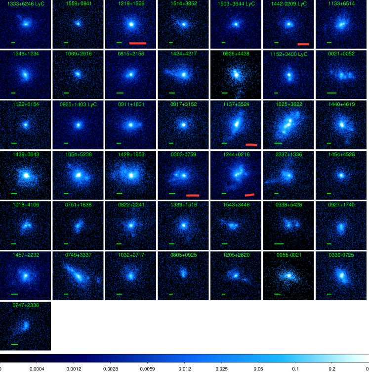
Figure 2.— The $3\hbox{${}^{\prime\prime}$}\times 3\hbox{${}^{\prime\prime}$}$ NUV images of Green Peas from the COS target acquisitions. In all panels, the colors are in log-scale with the same count-rates limits (from 0 to 0.4). These images are sorted by decreasing $f^{Ly\alpha}_{esc}$ from left to right, and from top to bottom. The label shows the ID of each Green Pea. The five LyC leakers are marked with ‘LyC’. The green bar in each panel shows the physical scale of 1 Kpc.

3. Ly$\alpha$ Equivalent Width and Escape Fraction

3.1. Measurements of Ly$\alpha$ flux, EW, and escape fraction

Most Green Peas in our sample show strong Ly$\alpha$ emission lines (figure 3). But about 1/3 Green Peas have relatively weak Ly$\alpha$ lines, where the Ly$\alpha$ absorptions in underlying continuum become non-negligible. Since we want to measure Ly$\alpha$ emission from the recombination of interstellar HI gas, we need to subtract the underlying continuum.

We first estimate a constant local continuum from wavelength ranges near Ly$\alpha$ where the spectra look flat and there are no obvious emission or absorption features. We calculate the “local continuum” $f_{\lambda}$(continuum) as the average of the spectra in these continuum ranges.

For 33 Green Peas without damped Ly$\alpha$ absorption (see Table 3), we subtract the “local continuum” and calculate the Ly$\alpha$ flux by integrating the spectra in wavelength range $\sim~{}1212-1221$ Å. Then we correct the Ly$\alpha$ flux for underlying stellar absorption. The equivalent width of stellar Ly$\alpha$ absorption mostly depends on the star formation history and age of the stellar population (Pena-Guerrero & Leitherer 2013). By comparing the H$\alpha$ EW of these Green Peas (about $300-900$Å) with model predictions of H$\alpha$ EW in star-forming galaxies, we found that these Green Peas probably have instantaneous starburst with a burst age of $4-5$ Myr (Levesque & Leitherer 2013). According to the model calculations in Pena-Guerrero & Leitherer (2013), the stellar Ly$\alpha$ absorption EW is about $-7$ Å. So we correct the Ly$\alpha$ fluxes of these 33 Green Peas by an EW=$-7$ Å absorption.

In another 8 Green Peas, the spectra show damped Ly$\alpha$ absorption wings and weak residual Ly$\alpha$ emission lines. The damped Ly$\alpha$ absorption is caused by interstellar absorption of the continuum and/or the Ly$\alpha$ absorption of the underlying stellar atmosphere continuum spectra. To measure flux of the residual Ly$\alpha$ emission, we subtract Ly$\alpha$ line spectra by a constant “absorbed continuum”. The “absorbed continuum” is estimated as the average in the wavelength range where the Ly$\alpha$ emission line meets the absorbed continuum. Then we integrate the Ly$\alpha$ line spectra to get Ly$\alpha$ flux. Since the above absorption correction already includes stellar Ly$\alpha$ absorption, we don’t need to correct the stellar absorption for these 8 Green Peas. Note that in some cases, the stellar absorption might have a very narrow component which is not fully corrected by this method.

In the remaining two Green Peas (GP0339$-$0725 and GP0747$+$2336), the Ly$\alpha$ lines are too weak and we didn’t detect Ly$\alpha$ emission.

Then we correct the measured Ly$\alpha$ fluxes for Milky Way extinction using the Fitzpatrick (1999) extinction law. The rest-frame EW(Ly$\alpha$) is calculated using the Ly$\alpha$ fluxes and the “local continuum” as EW(Ly$\alpha$)=flux(Ly$\alpha$)/$f_{\lambda}$(continuum)/(1+redshift). The Ly$\alpha$ escape fraction, $f^{Ly\alpha}_{esc}$, is defined as the ratio of the measured Ly$\alpha$ flux to the intrinsic Ly$\alpha$ flux. Assuming case-B recombination, the intrinsic Ly$\alpha$ flux is about 8.7 times dust extinction corrected H$\alpha$ flux (See Henry et al. 2015 for discussions about the factor 8.7). Thus the $f^{Ly\alpha}_{esc}$ is Ly$\alpha$(observed)/(8.7$\times H\alpha_{corrected}$). The SDSS H$\alpha$ spectra were taken with 3^′′ diameter aperture which matches the COS 2.5^′′ diameter aperture very well. Note that many Ly$\alpha$ galaxies have a very extended Ly$\alpha$ halo (e.g. Ostlin et al. 2009; Hayes et al. 2013; Momose et al. 2014). For these Green Pea galaxies, their Ly$\alpha$ to UV size ratios are about 2$-$4 (Yang et al. 2017). Thus COS 2.5^′′ aperture probably captured the majority of Ly$\alpha$ emission of those Green Peas.

Because the total counts per pixel in the UV continuum of this sample are small, we calculate the error spectra using the Poisson noise of the total counts. The statistical errors of Ly$\alpha$ fluxes are calculated from the error spectra using the error propagation formula. The Ly$\alpha$ flux, luminosity, EW(Ly$\alpha$), and $f^{Ly\alpha}_{esc}$ are shown in Table 3. A comparison of the $f^{Ly\alpha}_{esc}$ and EW(Ly$\alpha$) is shown in figure 4.

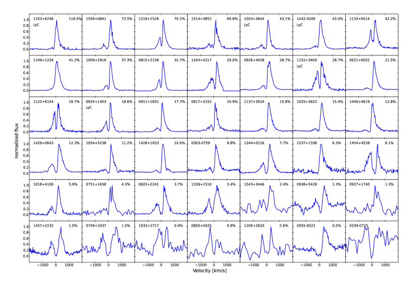
Figure 3.— Ly$\alpha$ emission line spectra of Green Peas before subtracting continuum. These 42 galaxies are sorted by decreasing $f^{Ly\alpha}_{esc}$ from left to right, and from top to bottom. The ID and $f^{Ly\alpha}_{esc}$ are given in each panel. The five LyC leakers are marked with ‘LyC’. The last one galaxy (GP0339$-$0725) shows weak Ly$\alpha$ absorption. One Green Pea (GP0747$+$2336) is not shown here, because its Ly$\alpha$ spectra is very noisy and no Ly$\alpha$ emission or absorption lines are detected.

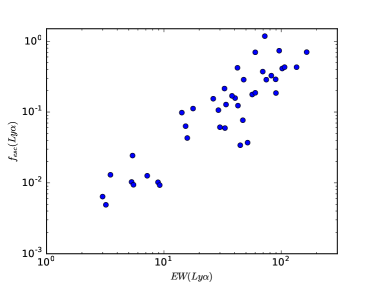
Figure 4.— Comparison of the $f^{Ly\alpha}_{esc}$ and EW(Ly$\alpha$) of Green Peas.

3.2. Ly$\alpha$ EW distribution of Green Peas

With a large sample of Green Peas that cover the whole ranges of dust and metallicity, we now have a more reliable estimation of the EW(Ly$\alpha$) distribution of Green Peas than previous result. 41 out of 43 Green Peas show Ly$\alpha$ emission lines. 28 out of 43 GPs (65%) in our sample have rest-frame EW(Ly$\alpha$) $\mathrel{\hbox{\hbox to0.0pt{\hbox{\lower 4.0pt\hbox{$\sim$}}\hss}\hbox{$>$}}}$ 20Å and would be classified as LAEs in a typical high-redshift narrow-band survey. We compared the EW(Ly$\alpha$) distribution of these 28 Green Peas to high redshift LAEs samples. The high redshift LAEs samples include a sample of $z=2.8$ narrow-band selected LAEs (Zheng et al. 2016) and a sample of spectroscopically confirmed LAEs at $z$=5.7 or 6.5 (Kashikawa et al. 2011). To be consistent with the methods used in high-$z$ LAEs studies, we use the EW(Ly$\alpha$) of Green Peas without correction of the stellar Ly$\alpha$ absorption. We also add a GALEX selected $z\sim 0.3$ LAE sample to the comparison (Deharveng et al. 2008; Cowie et al. 2011; Finkelstein et al. 2009; Scarlata et al. 2009). Figure 5 shows the cumulative EW(Ly$\alpha$) fraction distributions of these four samples. These 28 Green Peas have very similar EW(Ly$\alpha$) distribution to the high-redshift ($z=2.8$) sample. So Green Peas in general are the best nearby analogs of high-$z$ LAEs.

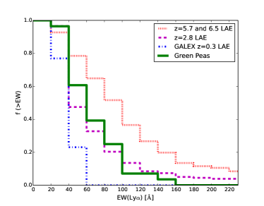
Figure 5.— Here we compare the rest-frame EW(Ly$\alpha$) distribution of Green Peas with different samples. The solid green line shows the sample of 28 Green Peas with EW(Ly$\alpha$) $\mathrel{\hbox{\hbox to0.0pt{\hbox{\lower 4.0pt\hbox{$\sim$}}\hss}\hbox{$>$}}}$ 20Å. The blue dash-dot line shows the GALEX $z\sim 0.3$ LAE sample (Cowie et al. 2011; Finkelstein et al. 2009; Scarlata et al. 2009). The magenta dashed line shows the $z=2.8$ LAE sample from Zheng et al. (2016). The red dotted line shows the $z=5.7$ and $6.5$ LAE sample from Kashikawa et al. (2011).

4. Ly$\alpha$ escape and Ly$\alpha$ profiles

4.1. Kinematic Features of Ly$\alpha$ Profile

In the Ly$\alpha$ escape process, Ly$\alpha$ photons are resonant scattered by the HI gas. Depending on the column density and bulk motion of HI gas, the resonant scatterings can significantly modify the Ly$\alpha$ profile. Therefore the Lya profile carries a lot of information about the HI gas properties. High-$z$ LAEs usually show an asymmetric or a double-peaked Ly$\alpha$ emission line profile (e.g. Rhoads et al 2003; Kashikawa et al. 2011; Erb et al. 2014). For LAEs with detected optical emission lines and systemic redshifts, the peaks of Ly$\alpha$ profiles are usually redshifted with respect to the systemic velocities (McLinden et al. 2011, 2014; Chonis et al. 2013; Hashimoto et al. 2013; Song et al. 2014; Shibuya et al. 2014; Erb et al. 2014). The velocity offset of Ly$\alpha$ emission line from the systemic velocity is usually smaller in LAEs than in continuum selected galaxies with weaker Ly$\alpha$ emission lines or Ly$\alpha$ absorptions (Shapley et al. 2003).

Most Green Peas show double-peaked Ly$\alpha$ profiles (figure 3). For a typical double-peaked profile, we define the “red peak” as the peak in the Ly$\alpha$ line profile occurring at velocity > 0, the “blue peak” as the Ly$\alpha$ peak at velocity < 0, and the “valley” as the flux minimum between the two peaks.

With a sample covering a large range of properties, we can see the Ly$\alpha$ profiles are diverse. In figure 3, the 42 Green Peas are sorted by decreasing $f^{Ly\alpha}_{esc}$ from top left to bottom right. Three Green Peas with high $f^{Ly\alpha}_{esc}$ show single peak profiles where the peak velocities are close to zero (GP1333$+$6246, GP1442$-$0209, and GP1249$+$1234). Many Green Peas with intermediate $f^{Ly\alpha}_{esc}$ generally show double-peaked profiles with much stronger red peaks than blue peaks. On the other hand, many Green Peas with low $f^{Ly\alpha}_{esc}$ have a relatively large ratio of blue peak to red peak.

As in Paper I, we measure four kinematic features of the Ly$\alpha$ profile: i) the blue peak velocity V(blue-peak); ii) the red peak velocity V(red-peak); iii) the peak separation V(red-peak)$-$V(blue-peak); and iv) the full width at half maximum (FWHM) of the red portion of Ly$\alpha$ profile, FWHM(red). The velocities are relative to the systemic redshift derived from SDSS spectra. The measurements of these kinematic features are shown in Table 3. For some Green Peas, we don’t measure their velocities because their Ly$\alpha$ profiles are too noisy. In the notes of Table 3, we explain the reason for each profile without velocity measurement. To measure the errors of velocity peaks, we use a Monte-Carlo method to generate 1000 fake spectra by adding Gaussian noise (with the error spectra as the $\sigma$ of Gaussian noise) to the observed spectra. Then we measure the peak velocities of these 1000 fake spectra and use the standard deviations as the errors. In summary, we have measurements of V(blue-peak) and the peak separation in 28 galaxies, and of V(red-peak) and FWHM(red) in 37 galaxies.

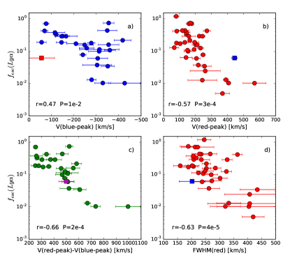
Figure 6.— Relations between $f^{Ly\alpha}_{esc}$ and the kinematic features of Ly$\alpha$ profile: (a) $f^{Ly\alpha}_{esc}$ and the blue peak velocity of Ly$\alpha$ profile, V(blue-peak); (b) $f^{Ly\alpha}_{esc}$ and the red peak velocity of Ly$\alpha$ profile, V(red-peak); (c) $f^{Ly\alpha}_{esc}$ and the peak separation of Ly$\alpha$ profile; (d) $f^{Ly\alpha}_{esc}$ and the FWHM of the red portion of Ly$\alpha$ profile, FWHM(red). The Spearman correlation coefficient and null probability are shown. GP1454+4528 with possible gas inflows is marked by a square in different color in each panel.

4.2. Relations between Ly$\alpha$ escape and Ly$\alpha$ kinematics

We show the relations between $f^{Ly\alpha}_{esc}$ and the kinematic features of Ly$\alpha$ profiles in figure 6. As $f^{Ly\alpha}_{esc}$ covers a range of about 3 dex, we show it in logarithmic scale. $f^{Ly\alpha}_{esc}$ shows anti-correlations with all four kinematic features – V(blue-peak), V(red-peak), the peak separation V(red-peak)$-$V(blue-peak), and the FWHM(red). We calculate the Spearman correlation coefficients of these relations (shown in each panel of figure 6).

In Paper I, we found the $f^{Ly\alpha}_{esc}$ correlates strongly with V(blue-peak). Here we can see most Green Peas still follow the correlation, but there are a few Green Peas with large scatter. So the overall correlation is worse than in Paper I. These outliers suggest that the Ly$\alpha$ blue peak velocities are determined by multiple mechanisms. For example, one outlier (GP1454+4528, marked with a square and different color in figure 6) has a distinct profile with the largest positive V(valley) (the velocity at the inter-peaks dip) and very strong blue portion Ly$\alpha$ emission. Its V(blue-peak) and V(red-peak) clearly offset from the trends. However, if we exchange the V(blue-peak) and V(red-peak), then it follows the trends very well. There is probably strong gas inflows as well as gas outflows in this galaxy. We excluded this object from the calculation of correlation coefficients.

On the other hand, in Paper I, we found large scatter between $f^{Ly\alpha}_{esc}$ and V(red-peak) with 12 Green Peas. However, as the current sample covers a large range of $f^{Ly\alpha}_{esc}$ and V(red-peak), $f^{Ly\alpha}_{esc}$ shows an anti-correlation with V(red-peak). The relation between $f^{Ly\alpha}_{esc}$ and V(red-peak) in this Green Peas sample is very similar to the relations between EW(Ly$\alpha$) and V(red-peak) in high redshift LAEs and LBGs, where the LAEs have high EW(Ly$\alpha$) and small V(red-peak), while the LBGs have small EW(Ly$\alpha$) and large V(red-peak) (Shapley et al. 2003; Hashimoto et al. 2013; Erb et al. 2014).

We also found that $f^{Ly\alpha}_{esc}$ anti-correlates with FWHM(red). We do a linear fit to this relation and get the following function.

$$log(f^{Ly\alpha}_{esc})=-0.545\times(FWHM(red)/100km/s)+0.563$$

The scatter of this relation is 0.43 dex in log($f^{Ly\alpha}_{esc}$). Since any high-$z$ LAE with a spectrum will have a measured FWHM for the red peak, it is easy to use this relation to infer the Ly$\alpha$ escape fraction of high-$z$ LAE.

Brief interpretations: The Ly$\alpha$ profile depends on the column density and the kinematics of HI gas. As the HI column density increases, the numbers of scatterings for Ly$\alpha$ photons increase. The more scatterings generally result in larger offsets of peak velocities (V(blue-peak) and V(red-peak)) and broader line profile (FWHM(red)). Also, more scatterings increase the Ly$\alpha$ photons’ path lengths which makes the Ly$\alpha$ radiation more susceptible to dust extinction and consequently decreases the Ly$\alpha$ escape fraction. Thus those anti-correlations mostly indicate that the $f^{Ly\alpha}_{esc}$ decreases as the column density of HI gas increases.

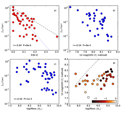
Figure 7.— a) Relation between $f^{Ly\alpha}_{esc}$ and dust extinction E(B-V). The black dashed (blue dotted) line shows the expected Ly$\alpha$ escape fraction if Ly$\alpha$ is only absorbed by dust following the Calzetti et al. (2000) extinction law (the SMC extinction law). b) Relation between $f^{Ly\alpha}_{esc}$ and the metallicity from $T_{e}$ method. c) Relation between $f^{Ly\alpha}_{esc}$ and stellar mass. The Spearman correlation coefficient and null probability are shown in panel a), b), and c). d) The mass-metallicity relation of this sample. The color-bar shows the value of log($f^{Ly\alpha}_{esc}$). The dashed line shows the mass-metallicity relation for SDSS galaxies in Amorin et al. (2010).

5. Ly$\alpha$ escape and other galactic properties

5.1. dust extinction, stellar mass, and metallicity

These Green Peas are very well studied galaxies and provide a great opportunity to explore the dependence of Ly$\alpha$ escape on other galactic properties. Previous studies have found that $f^{Ly\alpha}_{esc}$ anti-correlates with dust extinction (Atek et al. 2014; Cowie et al. 2011; Paper I). However the relation between $f^{Ly\alpha}_{esc}$ and metallicity are unclear (Finkelstein et al. 2011; Atek et al. 2014; Hayes et al. 2014; Paper I). Our sample covers the full ranges of dust extinction and metallicity of Green Peas. In figure 7, we show the relations between $f^{Ly\alpha}_{esc}$ and E(B-V), metallicity, and stellar mass. The Spearman correlation coefficients of these relations are shown figure 7.

The Green Peas with higher dust extinction tend to have smaller $f^{Ly\alpha}_{esc}$, confirming that dust extinction is an important factor in Ly$\alpha$ escape. In figure 7a, we also show the expected Ly$\alpha$ escape fractions if Ly$\alpha$ is only absorbed by dust following the Calzetti et al. (2000) extinction law (dashed line) or the SMC extinction law (Gordon et al. 2003) (dotted line). The SMC extinction law is steeper in FUV than the Calzetti et al. (2000) extinction law, so the extinction of Ly$\alpha$ emission is larger for SMC extinction law. Many Green Peas are below the dashed and dotted lines, because resonant scatterings increase the escape path length of Ly$\alpha$ photons and the chances of being absorbed by dust. Interestingly, many Green Peas are above the relation for SMC extinction law. If the dust extinction in Green Peas follows SMC extinction law, then it probably suggests resonant scatterings in clumpy dust distributions decrease the dust extinction of Ly$\alpha$ emission (Neufeld 1991; Hansen & Oh 2006; Finkelstein et al. 2009; Scarlata et al. 2009; but also see Laursen et al. 2013 showing that clumpy media does not decrease the dust extinction of Ly$\alpha$ for typical conditions in LAEs).

$f^{Ly\alpha}_{esc}$ also anti-correlates with metallicity and stellar mass. In the $f^{Ly\alpha}_{esc}$ vs. metallicity diagram, only 37 galaxies with [OIII]$\lambda$4363 line $S/N>3$ are shown. In figure 7, we also show the mass-metallicity relation of Green Peas and color the sample with $f^{Ly\alpha}_{esc}$. The dashed line shows the mass$-$metallicity relation for SDSS galaxies in Amorin et al. (2010), where the metallicity of SDSS galaxies are calculated with the same effective temperature method. These Green Peas have lower metallicities than the mass$-$metallicity relation of SDSS galaxies, similar to other emission line selected galaxies (Xia et al. 2012; Ly et al. 2014; Song et al. 2014). These Green Peas with lower metallicities and smaller masses have less dust extinction. In addition, ionized gas outflows can blow out the metal enriched gas and decrease the metallicity and dust extinction. At the same time, the ionized gas outflows can make holes with low HI column densities and help Ly$\alpha$ escape.

5.2. Morphology and size of UV emission

We get the NUV image of each object from the COS target acquisition (figure 2). So we also explore the relation between Ly$\alpha$ escape and the UV morphology. The pixel scale of NUV image is 0.0235 $\pm$ 0.0001 arcsec/pixel. The FWHM of point spread function is about 2 pixels or 0.047^′′. As we can see from the images, most Green Peas are very small and compact. Multiple clumps, tidal tails, and asymmetric shapes are common, which may suggest dwarf-dwarf mergers are common in Green Peas. In figure 2, these images are sorted by decreasing $f^{Ly\alpha}_{esc}$ from left to right, and from top to bottom. The $f^{Ly\alpha}_{esc}$ does not show an obvious relation with the morphology.

We then use GALFIT (Peng et al. 2010) to measure the galaxy size. We fit the image with a single Sersic profile component and get the half light radius of each galaxy. The half light radii are shown in Table 1. The relation between $f^{Ly\alpha}_{esc}$ and the half light radius has very large scatter.

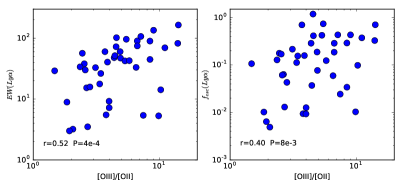
Figure 8.— Left: Relation between EW(Ly$\alpha$) and [OIII]/[OII]. Right: Relation between $f^{Ly\alpha}_{esc}$ and [OIII]/[OII]. [OIII]/[OII] is defined as ([OIII]$\lambda$4959+[OIII]$\lambda$5007)/([OII]$\lambda$3726+[OII]$\lambda$3729). The Spearman correlation coefficient and null probability are shown in each panel.

Figure 9.— The observed Ly$\alpha$ profiles (blue lines) and the best fit Ly$\alpha$ profiles (red lines) for 23 Green Peas with good S/N in their Ly$\alpha$ profiles. In Paper I, we showed the radiative transfer model fitting results of another 12 Green Peas. These galaxies are sorted by decreasing $f^{Ly\alpha}_{esc}$ from left to right, and from top to bottom.

5.3. [OIII]/[OII] ratio

Green Peas are selected to have large [OIII]/[OII] ratios. The [OIII]/[OII] ratio has been used to select LyC leaker candidates, and large [OIII]/[OII] may indicate the existence of paths with low HI optical depth (Jaskot & Oey 2014; Izotov et al. 2016). In figure 8, we show the relations of EW(Ly$\alpha$) vs. [OIII]/[OII] and $f^{Ly\alpha}_{esc}$ vs. [OIII]/[OII]. The Ly$\alpha$ line strength generally increases with [OIII]/[OII], but the scatter is large.

6. Ly$\alpha$ profile fitting

The Ly$\alpha$ emission line profiles can usually be explained by resonant scatterings of Ly$\alpha$ photons by an outflowing HI gas shell (e.g. Ahn et al. 2001; Verhamme et al. 2006; Dijkstra et al. 2006; Schaerer et al. 2011). To extract more information from the Ly$\alpha$ profiles and explore the physical process of Ly$\alpha$ escape, we fit the Ly$\alpha$ profiles with the outflowing HI shell radiative transfer model (Dijkstra et al. 2014; Gronke et al. 2015).

In the model, Ly$\alpha$ photons were generated by a source fully surrounded by a spherical dusty HI gas shell which scattered/absorbed the Ly$\alpha$ photons. The intrinsic Ly$\alpha$ line has a Gaussian profile with width $\sigma$. The shell is described by four parameters: (i) outflow velocity $v_{exp}$, (ii) HI column density $N_{HI}$, (iii) temperature T (including turbulent motion as well as the true temperature), and (iv) dust optical depth $\tau_{d}$. Generally, these parameters affect the Ly$\alpha$ profile as follows: a larger outflow velocity and a smaller $N_{HI}$ will decrease the red-peak velocity; a higher temperature will generally broaden the line profile; a larger dust optical depth will decrease the line strength. Then we find the best-fit model parameters ($\sigma$, $v_{exp}$, $N_{HI}$, T, $\tau_{d}$) and calculate the errors of parameters with Markov Chain Monte Carlo (MCMC) method. We refer the reader to Gronke et al. (2015) and Paper I for details of the model and the fitting method.

In Paper I, we showed the fitting results of 12 Green Peas. The model fit nine profiles very well, but failed in the other three profiles. Here we show the fitting results for another 23 Green Peas (out of the 31 additional Green Peas) with sufficient S/N in their Ly$\alpha$ profiles. The model fit the observed profiles very well in many cases (figure 9). The best fit parameters are shown in Table 4. We discussed a few interesting fitting results below.

(1) HI column density: In Paper I, we found $f^{Ly\alpha}_{esc}$ anti-correlates with the best fit $N_{HI}$ for the 12 Green Peas. Here we show the relation between $f^{Ly\alpha}_{esc}$ and the best fit $N_{HI}$ in figure 10 for the combined sample of 35 Green Peas. The result confirms the anti-correlation between $f^{Ly\alpha}_{esc}$ and $N_{HI}$. For the three cases (GP1424+4217, GP1133+6514, and GP1219+1526, marked by large blue circles) where the fitting procedure failed, we plot the $N_{HI}$ obtained by manually adjusting the model parameters to match the observed depth of the “valley” and the relative heights of blue and red peaks (see Section 6 of Paper I). For GP1454$+$4528 (marked by a red square) with gas inflow, the fitting was bad. For the two galaxies marked by large cyan triangles, the best fit $N_{HI}$ are not constrained. If the three galaxies marked by the square and triangle are excluded, the Spearman correlation coefficient for the relation of $f^{Ly\alpha}_{esc}$ and $N_{HI}$ is r=-0.59 (P=4e-4). If all six galaxies marked by the large circle, square and triangle are excluded, the Spearman correlation coefficient is r=-0.52 (P=4e-3). This result is consistent with studies of high redshift LAEs that suggested LAEs have lower $N_{HI}$ than non-LAEs (e.g. Shibuya et al. 2014; Erb et al. 2014; Hashimoto et al. 2015). Therefore the low column density of HI gas is a key factor to make Ly$\alpha$ escape.

Figure 10.— Relation between $f^{Ly\alpha}_{esc}$ and the best fit $N_{HI}$ from radiative transfer model. Five known LyC leakers are marked by large diamonds. For the three cases (GP1424+4217, GP1133+6514, and GP1219+1526, marked by large blue circles) where the fitting procedure failed, we plot the $N_{HI}$ obtained by manually adjusting the model parameters to match the observed depth of the “valley” and the relative heights of blue and red peaks (see Section 6 of Paper I). For GP1454$+$4528 (marked by a large red square) with gas inflow, the fitting is bad (see figure 8). For the two galaxies marked by large cyan triangles (GP1428$+$1653 and GP1122$+$6154), the best fit $N_{HI}$ are not constrained. The Spearman correlation coefficient is calculated without the three galaxies marked by square and triangle.

(2) Intrinsic Ly$\alpha$ line width: The intrinsic Ly$\alpha$ line Gaussian width $\sigma$ is about $2-3$ times larger than the H$\alpha$ Gaussian width in many cases, as we discussed in Paper I. In four cases, the best fit $\sigma$ is narrow and comparable to the H$\alpha$ width because the best fit profile only has a single peak. The wide intrinsic Ly$\alpha$ line profile can be due to important radiative transfer effects that broaden Ly$\alpha$ profile near to the source, before the processes attributed to the outflowing HI shell.

(3) Outflow velocities: The best fit shell outflow velocities are mostly between 5 to 170 km s^-1 which are generally smaller than the outflow velocities measured from the low-ionized UV absorption lines (Yang et al. in-prep). This may suggest the low-ionized absorption lines trace a different gas component from the HI gas. We also noticed that for six profiles with strong blue peaks, the best fit shell outflow velocities are smaller than 20 km s^-1. In GP1454$+$4528, the outlier discussed in section 4.1, the HI gas shell is inflowing with a best-fit velocity of $171$ km s^-1.

(4) The three failed cases: In Paper I, the model failed in three profiles with positive velocities at the line “valley”. We later improved the model by adding a shift of the velocity zero point as a free parameter of the fitting. The improved model can fit these three profiles very well. But the shifts of velocity zero points are about $90-150$ km s^-1 which are too large to be due to the errors of wavelength calibration. Those large shifts may be explained by some additional radiative transfer effects before the Ly$\alpha$ photons meet the HI gas shell.

Although the shell model captures many real radiative transfer effects and can fit the Ly$\alpha$ profiles very well, we should be cautious about the interpretation of the best fit parameters. A simple shell model can mimic more complex real physical properties (Gronke et al. 2016). For example, a low $N_{HI}$ model can mimic a model in which the gas is clumpy and the covering factor is low (Gronke & Dijkstra 2016). In this case, the best-fit $N_{HI}$ value is a simple approximation of the overall HI column densities. Interestingly, the best fit $N_{HI}$ of the five LyC leakers are about $10^{17-20}~{}cm^{-2}$, larger than the $N_{HI}$ that permit LyC escape. It suggests that their LyC emission probably escape through some holes in the interstellar medium with much lower $N_{HI}$.

Figure 11.— Top-left: the relation of E(B-V) vs. V(red-peak); The color-bar shows log($f^{Ly\alpha}_{esc}$) value. Top-right: the relation of $f^{Ly\alpha}_{esc}$ and E(B-V); The color-bar shows V(red-peak) value. Bottom-left: the comparison of observed and predicted $f^{Ly\alpha}_{esc}$. Here the predicted log($f^{Ly\alpha}_{esc}$)=$a\times(E(B-V)/0.1)+b\times(V(redpeak)/100)+c$. Bottom-right: the histogram of the differences, log($f^{Ly\alpha}_{esc}$)-log(predicted $f^{Ly\alpha}_{esc}$).

7. Predicting Ly$\alpha$ escape fraction

As we said in the Introduction, one major reason for the studies of Ly$\alpha$ escape is to use Ly$\alpha$ lines to probe reionization. A fraction ($f^{Ly\alpha}_{esc}$) of intrinsic Ly$\alpha$ photons first escape out of an LAE, then they go through the IGM where they can be further scattered by HI, and the remaining photons can finally be observed as a Ly$\alpha$ line. So the IGM transmission can be measured from the observed Ly$\alpha$ line flux if we know the intrinsic Ly$\alpha$ line flux and $f^{Ly\alpha}_{esc}$, i.e. $IGM\ Transmission=(Observed~{}Ly\alpha)/(Intrinsic~{}Ly\alpha~{}\times~{}$$f^{Ly\alpha}_{esc}$). In the near future, JWST will be able to measure the observed Ly$\alpha$ line and derive the intrinsic Ly$\alpha$ line from the observed H$\alpha$ line for galaxies in the epoch of reionization. If the remaining factor, $f^{Ly\alpha}_{esc}$, can be predicted from other observed galactic properties, then each Ly$\alpha$ line can be used as an IGM probe on its line of sight. With this sample of Green Peas, we have found correlations between $f^{Ly\alpha}_{esc}$ and Ly$\alpha$ kinematic features, dust extinction, metallicity, stellar mass, and HI column density. So can we select a few observable factors and fit an empirical relation to predict $f^{Ly\alpha}_{esc}$?

Physically, Ly$\alpha$ escape depends on the properties of dust and HI gas, so we should select the factors that can indicate the properties of dust and HI gas. Dust extinction is relatively easy to measure and could be a useful factor. The Ly$\alpha$ kinematic features strongly depend on the column density and kinematics of HI gas and could be another useful factor. Among a few Ly$\alpha$ kinematic features, the Ly$\alpha$ red-peak velocity is easier and more robust to measure than the blue-peak velocity which might be removed by absorption and the line width which depends on the spectra resolution. The other three factors – metallicity, stellar mass, and HI column density from fitting of Ly$\alpha$ profile – are difficult to measure and the uncertainties are large. Furthermore, both dust extinction and Ly$\alpha$ V(red-peak) show relatively tight anti-correlations with $f^{Ly\alpha}_{esc}$. So we fit an linear empirical relation to predict $f^{Ly\alpha}_{esc}$ from dust extinction and V(red-peak) of Ly$\alpha$ profile.

In figure 11, we first show the relations of $f^{Ly\alpha}_{esc}$, E(B-V), and V(red-peak). In the diagram of E(B-V) vs. V(red-peak), objects are color-coded by $f^{Ly\alpha}_{esc}$. We can see that (i) E(B-V) and V(red-peak) don’t show a correlation; (ii) the Green Peas with lower dust extinction and smaller V(red-peak) have larger $f^{Ly\alpha}_{esc}$. In the diagram of $f^{Ly\alpha}_{esc}$ vs. E(B-V), objects are color-coded by V(red-peak). Those Green Peas with large V(red-peak) generally have smaller $f^{Ly\alpha}_{esc}$ than the others with the same E(B-V). Then we fit 37 Green Peas with both V(red-peak) and E(B-V) measurements. Two Green Peas, GP1454$+$4528 with gas inflow and GP0749$+$3337 with the largest V(red-peak), are outliers of the fitting, so we remove these two objects. The final best-fit relation of 35 Green Peas is

$$log(f^{Ly\alpha}_{esc})=a\times(E(B-V)/0.1)+b\times(V(redpeak)/100)+c$$

, where $(a=-0.437,\ b=-0.483,\ c=0.464$). In the bottom two panels of figure 11, we compare the observed and the predicted $f^{Ly\alpha}_{esc}$ and show the histogram of the differences, log($f^{Ly\alpha}_{esc}$)-log(predicted $f^{Ly\alpha}_{esc}$). The standard deviation of this relation is 0.3 dex.

Now we have a relation to predict $f^{Ly\alpha}_{esc}$ from dust extinction and Ly$\alpha$ V(red-peak). If JWST measures the observed Ly$\alpha$ flux, observed H$\alpha$ flux, dust extinction, and Ly$\alpha$ V(red-peak) of a $z>7$ LAE, then we can infer the IGM transmission along this line of sight using the formula $IGM\ Transmission=(Observed~{}Ly\alpha)/(Intrinsic~{}Ly\alpha~{}\times~{}$$f^{Ly\alpha}_{esc}$), where the “Intrinsic Ly$\alpha$” is calculated from dust extinction corrected H$\alpha$ flux and $f^{Ly\alpha}_{esc}$ is calculated from the empirical relation.

The IGM measured by this method is the “true” IGM far from the LAE, which is in contrast to the circum-galactic medium (CGM). The “true” IGM only affects the strength of Ly$\alpha$ red peak by the damped absorption factor of $e^{-\tau}$, where $\tau$ is the optical depth of the IGM HI gas along the line of sight, and its effect on the velocity of the narrow Ly$\alpha$ red peak is negligible. Some simulations suggested that the HI gas in the CGM can be very close to the Ly$\alpha$ photons in frequency, so the CGM HI gas can resonantly scatter and/or absorb Ly$\alpha$ photons at V(red-peak)$<$160 km s^-1 (Laursen et al. 2011; Dijkstra 2014) and change the V(red-peak) of Ly$\alpha$ profile. In fact those scatterings by CGM are part of the Ly$\alpha$ escape process before Ly$\alpha$ photons reach the “true” IGM. So the influence of CGM gas is already considered in the empirical relation.

This empirical relation has important implications for reionization tests with Ly$\alpha$ lines. Some observations suggested that the fraction of Ly$\alpha$ emission line in Lyman-break galaxies drops rapidly at $z>6.5$ (e.g. Hayes et al. 2011; Tilvi et al. 2014; Pentericci et al. 2014). This could be due to small number statistics. But if this signal is real, it suggests either (i) the “true” IGM optical depth increases rapidly or (ii) the optical depth of ISM and CGM increases rapidly. Using our empirical relation, we can measure the optical depth of the “true” IGM and distinguish these two possibilities.

Some recent observations suggest that five $z\sim 7$ galaxies show very small velocity offsets about 20-150km s^-1 between Ly$\alpha$ and [CII] emission lines (Pentericci et al. 2016; Bradac et al. 2017). Those small V(red-peak) values may indicate that the Ly$\alpha$ escape fractions are high and the optical depths of ISM and CGM are small.

One caveat regards whether the empirical relation derived from low-$z$ analogs is applicable to high-$z$ LAEs. The properties of ISM and CGM likely evolve between the low-$z$ LAEs (Green Peas) and LAEs in the epoch of reionization. However, since the physics of Ly$\alpha$ resonant scattering is same in both low and high-$z$, increasing the HI gas column density in ISM probably doesn’t change how $N_{HI}$ affects Ly$\alpha$ profile. So the empirical relation is very likely applicable to $z>6$ LAEs.

8. Conclusion

We studied Ly$\alpha$ escape in a statistical sample of Green Peas with HST/COS Ly$\alpha$ spectra. About 2/3 Green Peas show strong Ly$\alpha$ emission lines. Many Green Peas show double-peaked Ly$\alpha$ line profiles, but the Ly$\alpha$ profiles are diverse. These Green Peas have well measured galactic properties from SDSS optical spectra, so we investigated the dependence of Ly$\alpha$ escape on dust extinction, metallicity, stellar mass, galaxy morphology, and [OIII]/[OII] ratio. We also fit their Ly$\alpha$ profiles with the HI shell radiative transfer model. Finally, we derived an empirical relation to predict Ly$\alpha$ escape fraction. Our major conclusions are as follows:

1. With a statistical sample of 43 Green Peas that cover the whole ranges of dust extinction and metallicity properties of Green Peas, we found about 2/3 of Green Peas are strong Ly$\alpha$ line emitters with distribution of EW(Ly$\alpha$) consistent with high-$z$ LAEs. This confirmed that Green Peas generally are the best analogs of high-$z$ LAEs in the nearby universe.

2. The $f^{Ly\alpha}_{esc}$ shows anti-correlations with a few Ly$\alpha$ kinematic features – the blue peak velocity, the red peak velocity, the peak separation, and the FWHM(red) of Ly$\alpha$ profile. These Ly$\alpha$ kinematic features are sensitive to the column density and the kinematics of HI gas. As more scatterings in HI gas can make the Ly$\alpha$ velocity offsets larger and the Ly$\alpha$ profile broader, these correlations strongly suggest low $N_{HI}$ and fewer scatterings help Ly$\alpha$ photons escape.

3. With a large sample, we found many correlations regarding the dependence of Ly$\alpha$ escape on galactic properties – $f^{Ly\alpha}_{esc}$ generally increases at lower dust extinction, lower metallicity, lower stellar mass, and higher [OIII]/[OII] ratio. $f^{Ly\alpha}_{esc}$ does not have an obvious relation with the UV morphology of Green Peas.

4. The single shell radiative transfer model can reproduce most Ly$\alpha$ profiles of Green Peas. The best-fit $N_{HI}$ anti-correlates with $f^{Ly\alpha}_{esc}$, indicating that low $N_{HI}$ is key to Ly$\alpha$ escape.

5. We fit an empirical linear relation between $f^{Ly\alpha}_{esc}$, dust extinction, and Ly$\alpha$ red peak velocity. This relation can be used to predict the $f^{Ly\alpha}_{esc}$ of LAEs and isolate the effect of IGM scatterings from Ly$\alpha$ escape. As JWST can measure the dust extinction and Ly$\alpha$ red peak velocity of some $z>7$ LAEs, this relation makes it possible to measure the HI column density of IGM along the line of sight of each LAE and to probe reionization with their Ly$\alpha$ lines.

Table 1The Sample

ID	RA	DEC	z	E(B-V)MW	E(B-V)	12+log(O/H)	log(M/M⊙)	SFR	$R_{e}$	GO#
(1)	(2)	(3)	(4)	(5)	(6)	(7)	(8)	(9)	(10)	(11)
1333$+$6246a	13:33:03.94	$+$62:46:03.7	0.31812	0.017	0.000	7.72	8.50	1.4	0.72	13744
1559$+$0841	15:59:25.97	$+$08:41:19.1	0.29704	0.033	0.000	8.04	8.97	3.5	0.47	14201
1219$+$1526	12:19:03.98	$+$15:26:08.5	0.19560	0.022	0.000	7.81	8.35	13.0	0.33	12928
1514$+$3852	15:14:08.63	$+$38:52:07.3	0.33262	0.019	0.000	8.12	9.32	6.4	0.67	14201
1503$+$3644a	15:03:42.82	$+$36:44:50.8	0.35569	0.013	0.007	8.01	8.22	12.9	0.52	13744
1442$-$0209a	14:42:31.37	$-$02:09:52.8	0.29367	0.046	0.094	7.95	8.96	21.2	0.50	13744
1133$+$6514	11:33:03.80	$+$65:13:41.3	0.24140	0.009	0.040	7.95	9.30	6.4	0.82	12928
1249$+$1234	12:48:34.64	$+$12:34:02.9	0.26339	0.026	0.084	8.10	9.05	18.3	0.71	12928
1009$+$2916	10:09:18.99	$+$29:16:21.5	0.22192	0.019	0.000	7.92	7.87	3.7	0.46	14201
0815$+$2156	08:15:52.00	$+$21:56:23.6	0.14095	0.035	0.014	7.96	8.71	4.4	0.35	13293
1424$+$4217	14:24:05.73	$+$42:16:46.3	0.18479	0.009	0.028	8.02	8.34	19.2	0.48	12928
0926$+$4428	09:26:00.44	$+$44:27:36.5	0.18069	0.016	0.074	8.02	8.78	14.8	0.43	11727
1152$+$3400a	11:52:04.88	$+$34:00:49.8	0.34195	0.017	0.114	7.95	8.35	23.2	0.52	13744
0021$+$0052	00:21:01.02	$+$00:52:48.1	0.09836	0.021	0.038	8.14	9.30	13.7	0.44	13017
1122$+$6154	11:22:19.73	$+$61:54:45.4	0.20456	0.007	0.129	8.14	7.85	6.5	0.32	14201
0925$+$1403a	09:25:32.37	$+$14:03:13.0	0.30121	0.027	0.134	8.01	8.46	23.8	0.42	13744
0911$+$1831	09:11:13.34	$+$18:31:08.2	0.26220	0.024	0.168	7.96	9.75	26.8	0.57	12928
0917$+$3152	09:17:02.52	$+$31:52:20.5	0.30036	0.017	0.189	8.10	9.37	21.8	0.47	14201
1137$+$3524	11:37:22.14	$+$35:24:26.7	0.19439	0.016	0.043	8.12	9.56	19.5	0.72	12928
1025$+$3622	10:25:48.38	$+$36:22:58.4	0.12649	0.010	0.088	8.11	9.20	10.0	0.76	13017
1440$+$4619	14:40:09.94	$+$46:19:36.9	0.30076	0.012	0.148	8.13	9.62	38.0	0.72	14201
1429$+$0643	14:29:47.03	$+$06:43:34.9	0.17351	0.022	0.053	8.01	9.40	30.6	0.40	13017
1054$+$5238	10:53:30.83	$+$52:37:52.9	0.25264	0.013	0.069	8.08	9.77	27.3	0.62	12928
1428$+$1653	14:28:56.41	$+$16:53:39.4	0.18164	0.017	0.175	8.12	9.60	22.2	0.77	13017
0303$-$0759	03:03:21.41	$-$07:59:23.2	0.16488	0.085	0.000	7.87	9.15	8.9	0.56	12928
1244$+$0216	12:44:23.37	$+$02:15:40.4	0.23943	0.021	0.062	8.09	9.65	31.0	1.02	12928
2237$+$1336	22:37:35.05	$+$13:36:47.0	0.29350	0.049	0.126	8.11	9.45	30.7	1.08	14201
1454$+$4528	14:54:35.58	$+$45:28:56.3	0.26851	0.036	0.169	8.22	9.52	21.4	0.45	14201
1018$+$4106	10:18:03.24	$+$41:06:21.0	0.23705	0.012	0.094	7.93	9.32	10.4	0.78	14201
0751$+$1638	07:51:57.78	$+$16:38:13.2	0.26471	0.031	0.149	7.85	8.35	7.8	0.80	14201
0822$+$2241	08:22:47.66	$+$22:41:44.0	0.21619	0.039	0.195	8.11	8.43	41.6	0.68	14201
1339$+$1516	13:39:28.30	$+$15:16:42.1	0.19202	0.026	0.114	8.05	9.43	18.7	0.38	14201
1543$+$3446	15:43:01.22	$+$34:46:01.4	0.18733	0.025	0.000	7.96	8.05	2.6	0.77	14201
0938$+$5428	09:38:13.49	$+$54:28:25.0	0.10208	0.015	0.123	8.17	9.40	13.6	0.47	11727
0927$+$1740	09:27:28.67	$+$17:40:18.6	0.28831	0.026	0.180	8.06	9.26	18.2	0.94	14201
1457$+$2232	14:57:35.13	$+$22:32:01.7	0.14861	0.041	0.061	8.02	9.13	11.6	0.42	13293
0749$+$3337	07:49:36.77	$+$33:37:16.3	0.27318	0.048	0.203	8.18	9.49	62.3	1.47	14201
1032$+$2717	10:32:26.95	$+$27:17:55.2	0.19246	0.018	0.097	8.22	9.65	13.3	0.63	14201
0805$+$0925	08:05:18.04	$+$09:25:33.5	0.33034	0.018	0.402	7.98	9.36	22.9	0.81	14201
1205$+$2620	12:05:00.67	$+$26:20:47.7	0.34261	0.016	0.178	7.89	9.84	22.0	0.83	14201
0055$-$0021	00:55:27.46	$-$00:21:48.7	0.16745	0.022	0.217	8.18	9.70	30.4	0.46	11727
0339$-$0725	03:39:47.79	$-$07:25:41.2	0.26071	0.053	0.095	8.31	9.70	29.6	0.88	14201
0747$+$2336	07:47:58.00	$+$23:36:32.7	0.15524	0.051	0.085	8.02	9.06	5.9	0.59	14201

Note. — Column Descriptions: (1) Object ID; (4) Redshifts are from SDSS optical spectra; (5) The Milky Way extinction $E(B-V)_{MW}$, based on Schlafly & Finkbeiner (2011); (6) dust extinction; (7) metallicity; (8) stellar mass; (9) star formation rate in unit of M${}_{\odot}~{}yr^{-1}$ derived from H$\alpha$ luminosity; (10) half light radius in unit of Kpc; (11) HST programs: GO14201 (PI S. Malhotra), GO13744 (PI T. Thuan; Izotov et al. 2016), GO13293 (PI A. Jaskot; Jaskot et al. 2014), GO12928 (PI A. Henry; Henry et al. 2015), GO11727 and GO13017 (PI T. Heckman; Heckman et al. 2011; Alexandroff et al. 2015). These 43 galaxies are sorted by decreasing $f^{Ly\alpha}_{esc}$ from top to bottom. The machine readable table is available online.

Table 2The line measurements from SDSS spectra

ID	[OII]3727	[OIII]4363	H$\beta$	[OIII]4959	[OIII]5007	H$\alpha$	EW(H$\alpha$)	[OIII]/[OII]
(1)	(2)	(3)	(4)	(5)	(6)	(7)	(8)	(9)
1333$+$6246	115$\pm$5	13.6$\pm$2.7	58$\pm$4	129$\pm$2	390$\pm$6	78$\pm$4	538	4.5
1559$+$0841	169$\pm$4	9.4$\pm$1.3	124$\pm$12	229$\pm$2	693$\pm$6	232$\pm$11	288	5.5
1219$+$1526	467$\pm$8	108.8$\pm$4.9	776$\pm$9	1635$\pm$8	4953$\pm$25	2207$\pm$18	744	14.2
1514$+$3852	270$\pm$5	9.2$\pm$3.1	139$\pm$3	248$\pm$2	751$\pm$6	327$\pm$6	232	3.7
1503$+$3644	220$\pm$3	19.3$\pm$1.6	184$\pm$2	397$\pm$2	1203$\pm$7	534$\pm$21	921	7.1
1442$-$0209	248$\pm$5	32.2$\pm$2.4	299$\pm$4	647$\pm$5	1960$\pm$14	988$\pm$13	858	9.0
1133$+$6514	268$\pm$5	19.2$\pm$2.3	196$\pm$3	376$\pm$2	1138$\pm$7	592$\pm$6	263	5.3
1249$+$1234	575$\pm$8	28.8$\pm$2.4	364$\pm$5	740$\pm$5	2242$\pm$14	1169$\pm$12	717	4.6
1009$+$2916	139$\pm$4	22.0$\pm$2.3	173$\pm$4	382$\pm$3	1156$\pm$9	473$\pm$16	422	11.1
0815$+$2156	293$\pm$5	56.4$\pm$3.3	462$\pm$5	1065$\pm$7	3227$\pm$22	1383$\pm$13	717	14.0
1424$+$4217	1129$\pm$16	114.9$\pm$3.6	1119$\pm$11	2463$\pm$11	7459$\pm$33	3333$\pm$25	629	8.4
0926$+$4428	1090$\pm$14	56.3$\pm$3.5	733$\pm$8	1318$\pm$7	3994$\pm$22	2314$\pm$18	437	4.4
1152$+$3400	237$\pm$4	22.5$\pm$1.3	228$\pm$3	461$\pm$2	1397$\pm$7	756$\pm$5	497	6.7
0021$+$0052	5172$\pm$29	127.8$\pm$6.7	2909$\pm$14	4275$\pm$12	12949$\pm$36	8855$\pm$32	320	3.1
1122$+$6154	257$\pm$5	11.6$\pm$1.3	200$\pm$4	369$\pm$3	1118$\pm$10	667$\pm$10	495	4.9
0925$+$1403	297$\pm$7	25.8$\pm$4.0	282$\pm$4	596$\pm$4	1806$\pm$11	960$\pm$10	633	6.7
0911$+$1831	576$\pm$10	15.5$\pm$3.2	379$\pm$5	442$\pm$3	1340$\pm$9	1343$\pm$14	348	2.5
0917$+$3152	300$\pm$5	6.2$\pm$2.3	210$\pm$3	244$\pm$1	739$\pm$4	760$\pm$7	250	2.5
1137$+$3524	1519$\pm$17	51.1$\pm$2.7	941$\pm$10	1563$\pm$7	4733$\pm$21	2865$\pm$21	434	3.9
1025$+$3622	1816$\pm$17	60.7$\pm$4.5	1038$\pm$10	1746$\pm$10	5289$\pm$31	3318$\pm$25	312	3.4
1440$+$4619	895$\pm$11	19.5$\pm$3.0	441$\pm$5	637$\pm$4	1929$\pm$12	1513$\pm$14	325	2.4
1429$+$0643	2245$\pm$23	152.3$\pm$6.8	1785$\pm$15	3503$\pm$15	10610$\pm$46	5524$\pm$37	686	5.8
1054$+$5238	1068$\pm$13	32.5$\pm$3.3	661$\pm$7	982$\pm$6	2974$\pm$17	2068$\pm$16	304	3.4
1428$+$1653	1574$\pm$17	19.6$\pm$3.0	706$\pm$8	733$\pm$4	2220$\pm$13	2511$\pm$20	261	1.5
0303$-$0759	488$\pm$8	74.0$\pm$2.5	656$\pm$7	1301$\pm$8	3941$\pm$23	1963$\pm$18	608	10.3
1244$+$0216	1252$\pm$12	64.1$\pm$3.3	853$\pm$7	1681$\pm$8	5091$\pm$25	2665$\pm$18	667	4.9
2237$+$1336	733$\pm$9	19.3$\pm$2.7	376$\pm$4	587$\pm$4	1780$\pm$11	1291$\pm$12	353	2.6
1454$+$4528	498$\pm$8	9.2$\pm$3.2	293$\pm$4	401$\pm$3	1215$\pm$8	1033$\pm$11	277	2.6
1018$+$4106	292$\pm$5	28.5$\pm$1.9	263$\pm$3	539$\pm$3	1633$\pm$10	846$\pm$8	570	6.5
0751$+$1638	216$\pm$6	10.7$\pm$3.6	115$\pm$3	187$\pm$2	567$\pm$5	401$\pm$7	299	2.8
0822$+$2241	1063$\pm$11	54.0$\pm$3.1	781$\pm$6	1551$\pm$6	4699$\pm$19	2886$\pm$17	605	4.4
1339$+$1516	602$\pm$8	61.4$\pm$3.2	667$\pm$7	1485$\pm$6	4499$\pm$18	2222$\pm$57	523	8.4
1543$+$3446	185$\pm$6	15.4$\pm$2.3	194$\pm$5	343$\pm$4	1037$\pm$11	480$\pm$7	342	7.5
0339$-$0725	978$\pm$12	14.7$\pm$2.3	538$\pm$6	733$\pm$4	2220$\pm$13	1786$\pm$15	345	2.6
0938$+$5428	3305$\pm$28	67.9$\pm$4.0	1887$\pm$15	2627$\pm$13	7957$\pm$39	6313$\pm$39	353	2.7
0927$+$1740	328$\pm$6	17.7$\pm$2.1	196$\pm$4	419$\pm$3	1268$\pm$9	707$\pm$9	707	4.0
1457$+$2232	764$\pm$9	103.1$\pm$2.7	868$\pm$12	2096$\pm$12	6349$\pm$36	2758$\pm$20	707	9.9
0749$+$3337	1312$\pm$14	20.3$\pm$2.4	652$\pm$7	811$\pm$5	2457$\pm$14	2447$\pm$27	361	1.9
1032$+$2717	845$\pm$8	25.1$\pm$0.8	520$\pm$5	910$\pm$4	2757$\pm$13	1687$\pm$13	651	3.8
0805$+$0925	73$\pm$5	4.3$\pm$3.5	72$\pm$4	123$\pm$3	371$\pm$8	333$\pm$6	353	4.0
1205$+$2620	324$\pm$5	9.0$\pm$3.7	165$\pm$3	198$\pm$1	599$\pm$4	587$\pm$8	350	1.9
0055$-$0021	1738$\pm$11	29.0$\pm$3.0	956$\pm$5	1197$\pm$3	3626$\pm$10	3587$\pm$12	249	2.1
0747$+$2336	363$\pm$5	35.8$\pm$1.8	354$\pm$5	796$\pm$5	2411$\pm$16	1166$\pm$11	366	7.6

Note. — Observed line fluxes from SDSS spectra in units of $10^{-17}$ erg s^-1 cm^-2. The EW(H$\alpha$) is rest-frame H$\alpha$ equivalent width. The [OIII]/[OII] ratio are extinction corrected using the Calzetti et al. (2000) extinction law. The machine readable table is available online.

Table 3Ly$\alpha$ properties

ID	Ly$\alpha$ flux	log(L(Ly$\alpha$) erg s-1)	EW(Ly$\alpha$)	$f^{Ly\alpha}_{esc}$	V(blue-peak)	V(red-peak)	FWHM(red)
	$10^{-16}$ erg s-1 cm-2		Å		km s-1	km s-1	km s-1
(1)	(2)	(3)	(4)	(5)	(6)	(7)	(8)
1333$+$6246a	160.4$\pm$2.8	42.7	72.3	1.180	$-^{d}$	79$\pm$17	245$\pm$24
1559$+$0841	145.0$\pm$3.1	42.6	96.0	0.735	$-$355$\pm$24	168$\pm$17	188$\pm$29
1219$+$1526	1345.3$\pm$5.9	43.2	164.5	0.702	$-$76$\pm$13	176$\pm$13	213$\pm$18
1514$+$3852	180.8$\pm$4.1	42.8	60.0	0.698	$-^{e}$	159$\pm$17	222$\pm$58
1503$+$3644a	195.2$\pm$4.3	42.9	106.6	0.431	$-$349$\pm$43	118$\pm$23	229$\pm$27
1442$-$0209a	504.5$\pm$5.6	43.1	134.9	0.430	$-^{d}$	135$\pm$26	267$\pm$25
1133$+$6514	208.0$\pm$1.9	42.6	42.3	0.422	$-$69$\pm$15	271$\pm$22	234$\pm$21
1249$+$1234	528.0$\pm$2.6	43.1	101.8	0.412	$-^{d}$	83$\pm$27	364$\pm$17
1009$+$2916	142.8$\pm$2.5	42.3	69.5	0.373	$-$116$\pm$45	144$\pm$22	206$\pm$26
0815$+$2156	401.2$\pm$1.4	42.3	82.2	0.327	$-$121$\pm$13	144$\pm$13	216$\pm$19
1424$+$4217	858.6$\pm$4.1	42.9	89.5	0.290	$-$150$\pm$32	224$\pm$10	208$\pm$16
0926$+$4428	636.8$\pm$2.3	42.8	47.8	0.287	$-$165$\pm$51	244$\pm$17	327$\pm$18
1152$+$3400a	248.6$\pm$4.6	43.0	74.5	0.287	$-$146$\pm$26	158$\pm$44	235$\pm$30
0021$+$0052	1523.5$\pm$9.7	42.6	32.8	0.215	$-$418$\pm$38	164$\pm$12	253$\pm$16
1122$+$6154	144.1$\pm$2.1	42.2	60.0	0.187	$-$56$\pm$21	194$\pm$26	202$\pm$25
0925$+$1403a	225.1$\pm$4.1	42.8	90.0	0.186	$-$145$\pm$24	133$\pm$23	160$\pm$25
0911$+$1831	315.7$\pm$2.1	42.8	56.5	0.177	$-$278$\pm$17	81$\pm$12	207$\pm$17
0917$+$3152	167.7$\pm$3.3	42.7	38.0	0.169	$-$209$\pm$42	104$\pm$22	189$\pm$25
1137$+$3524	381.1$\pm$3.4	42.6	40.4	0.158	$-$355$\pm$46	201$\pm$22	285$\pm$20
1025$+$3622	436.6$\pm$3.6	42.3	26.3	0.154	$-$248$\pm$39	210$\pm$12	253$\pm$15
1440$+$4619	214.2$\pm$3.6	42.8	33.8	0.128	$-^{d}$	67$\pm$29	248$\pm$30
1429$+$0643	607.1$\pm$2.9	42.7	42.7	0.123	$-$257$\pm$34	231$\pm$19	324$\pm$19
1054$+$5238	153.5$\pm$2.6	42.5	17.7	0.112	$-$314$\pm$88	192$\pm$12	225$\pm$25
1428$+$1653	311.9$\pm$2.2	42.5	29.1	0.106	$-$360$\pm$25	150$\pm$20	242$\pm$18
0303$-$0759	99.6$\pm$2.1	41.9	14.2	0.098	$-$313$\pm$48	153$\pm$26	270$\pm$23
1244$+$0216	189.9$\pm$1.6	42.5	47.0	0.077	$-$240$\pm$14	247$\pm$14	302$\pm$25
2237$+$1336	51.4$\pm$2.6	42.1	15.3	0.063	$-^{d}$	141$\pm$36	272$\pm$35
1454$+$4528	72.3$\pm$2.1	42.2	30.0	0.061	$-$56$\pm$58	444$\pm$18	202$\pm$47
1018$+$4106	47.0$\pm$1.5	41.9	33.1	0.059	$-$306$\pm$44	206$\pm$25	238$\pm$32
0751$+$1638	13.9$\pm$1.3	41.5	15.8	0.043	$-^{e}$	$-^{e}$	$-^{e}$
0822$+$2241	156.5$\pm$2.9	42.3	51.6	0.037	$-$304$\pm$65	217$\pm$31	262$\pm$39
1339$+$1516	82.5$\pm$1.9	41.9	44.7	0.034	$-$351$\pm$30	256$\pm$42	435$\pm$62
1543$+$3446b	10.6$\pm$0.8	41.0	5.4	0.024	$-^{e}$	261$\pm$94	407$\pm$90
0938$+$5428b	107.1$\pm$2.0	41.5	3.5	0.013	$-$279$\pm$20	390$\pm$17	333$\pm$43
0927$+$1740b	14.0$\pm$1.1	41.6	7.2	0.013	$-^{e}$	242$\pm$91	408$\pm$150
1457$+$2232b	32.3$\pm$0.6	41.3	5.3	0.010	$-$329$\pm$37	406$\pm$14	321$\pm$54
0749$+$3337	9.2$\pm$1.7	41.3	8.9	0.010	$-$427$\pm$72	568$\pm$72	405$\pm$114
1032$+$2717b	19.2$\pm$0.9	41.3	5.5	0.009	$-^{e}$	$-^{e}$	$-^{e}$
0805$+$0925b	9.5$\pm$1.3	41.5	9.2	0.009	$-^{e}$	$-^{e}$	$-^{e}$
1205$+$2620b	5.8$\pm$1.3	41.4	3.0	0.006	$-^{e}$	$-^{e}$	$-^{e}$
0055$-$0021b	31.3$\pm$1.0	41.4	3.2	0.005	$-^{e}$	368$\pm$45	420$\pm$39
0339$-$0725c	$-$1.4$\pm$1.8	$-$	$-$	$-$	$-$	$-$	$-$
0747$+$2336c	$-$	$-$	$-$	$-$	$-$	$-$	$-$

Note. — Column Descriptions: (1) Object ID; (2) Ly$\alpha$ emission line flux; (3) Ly$\alpha$ emission line luminosity; (4) equivalent width of Ly$\alpha$ line; (5) Ly$\alpha$ escape fraction; (6) Velocity of Ly$\alpha$ blue peak; (7) Velocity of Ly$\alpha$ red peak; (8) FWHM of the red portion of Ly$\alpha$ profile. These 43 galaxies are sorted by decreasing $f^{Ly\alpha}_{esc}$ from top to bottom. The machine readable table is available online.

Table 4Ly$\alpha$ profile Model Parameters

ID	log($N_{HI}~{}cm^{-2}$)	$V_{exp}$	log(T)	$\tau_{d}$	$\sigma$
		(km s-1)	(K)		km s-1
(1)	(2)	(3)	(4)	(5)	(6)
1333$+$6246	19.39${}^{+0.08}_{-0.07}$	270${}^{+4}_{-4}$	5.0${}^{+0.2}_{-0.1}$	0.71${}^{+0.09}_{-0.08}$	125${}^{+2}_{-2}$
1559$+$0841	19.40${}^{+0.07}_{-0.07}$	90${}^{+3}_{-4}$	3.0${}^{+0.1}_{-0.1}$	0.64${}^{+0.08}_{-0.06}$	203${}^{+2}_{-2}$
1514$+$3852	19.20${}^{+0.07}_{-0.07}$	80${}^{+4}_{-3}$	3.8${}^{+0.1}_{-0.1}$	0.01${}^{+0.01}_{-0.00}$	305${}^{+7}_{-7}$
1503$+$3644	16.81${}^{+0.08}_{-0.08}$	140${}^{+4}_{-4}$	5.4${}^{+0.2}_{-0.1}$	0.14${}^{+0.07}_{-0.05}$	266${}^{+5}_{-5}$
1442$-$0209	18.80${}^{+0.07}_{-0.07}$	150${}^{+4}_{-4}$	4.2${}^{+0.2}_{-0.2}$	0.01${}^{+0.01}_{-0.00}$	230${}^{+2}_{-2}$
1009$+$2916	19.60${}^{+0.07}_{-0.07}$	30${}^{+4}_{-4}$	3.4${}^{+0.1}_{-0.1}$	0.00${}^{+0.00}_{-0.00}$	201${}^{+3}_{-3}$
1152$+$3400	20.00${}^{+0.07}_{-0.07}$	5${}^{+1}_{-1}$	3.4${}^{+0.2}_{-0.1}$	0.01${}^{+0.00}_{-0.00}$	333${}^{+6}_{-6}$
0021$+$0052	19.59${}^{+0.07}_{-0.07}$	130${}^{+4}_{-3}$	5.0${}^{+0.1}_{-0.1}$	0.22${}^{+0.01}_{-0.01}$	100${}^{+2}_{-2}$
1122$+$6154	19.98${}^{+0.08}_{-1.85}$	7${}^{+1}_{-26}$	3.4${}^{+0.2}_{-0.2}$	0.00${}^{+1.13}_{-0.00}$	259${}^{+4}_{-5}$
0925$+$1403	19.79${}^{+0.07}_{-0.08}$	8${}^{+1}_{-1}$	3.0${}^{+0.2}_{-0.2}$	0.03${}^{+0.00}_{-0.00}$	229${}^{+5}_{-5}$
0917$+$3152	19.00${}^{+0.07}_{-0.07}$	60${}^{+3}_{-3}$	3.5${}^{+0.3}_{-0.2}$	0.01${}^{+0.01}_{-0.01}$	275${}^{+8}_{-8}$
1025$+$3622	19.40${}^{+0.07}_{-0.07}$	110${}^{+3}_{-4}$	4.1${}^{+0.2}_{-0.3}$	0.00${}^{+0.01}_{-0.00}$	228${}^{+7}_{-5}$
1440$+$4619	19.18${}^{+0.08}_{-0.08}$	259${}^{+4}_{-4}$	5.0${}^{+0.1}_{-0.1}$	0.23${}^{+0.03}_{-0.03}$	117${}^{+2}_{-2}$
1429$+$0643	20.39${}^{+0.08}_{-0.08}$	15${}^{+2}_{-2}$	3.4${}^{+0.1}_{-0.1}$	0.00${}^{+0.00}_{-0.00}$	392${}^{+3}_{-3}$
1428$+$1653	16.04${}^{+1.55}_{-0.09}$	168${}^{+5}_{-11}$	5.7${}^{+0.2}_{-0.4}$	0.10${}^{+0.02}_{-0.09}$	205${}^{+20}_{-4}$
2237$+$1336	19.88${}^{+0.15}_{-0.13}$	258${}^{+44}_{-10}$	4.9${}^{+0.2}_{-1.1}$	1.14${}^{+0.86}_{-0.33}$	140${}^{+12}_{-8}$
1454$+$4528	16.44${}^{+0.36}_{-0.09}$	-171${}^{+4}_{-4}$	5.4${}^{+0.1}_{-0.1}$	4.78${}^{+0.17}_{-0.34}$	427${}^{+10}_{-8}$
1018$+$4106	19.60${}^{+0.07}_{-0.07}$	49${}^{+4}_{-4}$	3.8${}^{+0.2}_{-0.2}$	0.07${}^{+0.04}_{-0.04}$	268${}^{+12}_{-11}$
0751$+$1638	19.39${}^{+0.07}_{-0.08}$	121${}^{+17}_{-20}$	4.4${}^{+0.3}_{-1.3}$	0.17${}^{+0.34}_{-0.13}$	326${}^{+31}_{-29}$
0822$+$2241	20.54${}^{+0.11}_{-0.18}$	6${}^{+3}_{-2}$	3.0${}^{+0.1}_{-0.2}$	0.01${}^{+0.02}_{-0.00}$	363${}^{+10}_{-19}$
1339$+$1516	19.00${}^{+0.07}_{-0.07}$	100${}^{+4}_{-4}$	3.1${}^{+0.6}_{-0.2}$	4.86${}^{+0.11}_{-0.23}$	345${}^{+5}_{-5}$
0938$+$5428	20.60${}^{+0.08}_{-0.08}$	15${}^{+2}_{-2}$	4.6${}^{+0.2}_{-0.2}$	0.08${}^{+0.01}_{-0.01}$	64${}^{+15}_{-10}$
0055$-$0021	20.40${}^{+0.07}_{-0.07}$	60${}^{+3}_{-4}$	4.2${}^{+0.1}_{-0.1}$	0.07${}^{+0.02}_{-0.02}$	322${}^{+17}_{-17}$

Note. — Column Descriptions: (2) HI column density of the outflowing HI shell; (3) outflowing velocity of the HI shell; (4) HI gas temperature including turbulent motion as well as the true temperature; (5) dust optical depth; (6) 1$\sigma$ width of the Gaussian profile of the intrinsic Ly$\alpha$ line. These 23 galaxies are sorted by decreasing $f^{Ly\alpha}_{esc}$ from top to bottom.

References

- Ahn et al. (2001) Ahn, S.-H., Lee, H.-W., & Lee, H. M. 2001, ApJ, 554, 604
- Amorín et al. (2010) Amorín, R. O., Pérez-Montero, E., & Vílchez, J. M. 2010, ApJ, 715, L128
- Alexandroff et al. (2015) Alexandroff, R. M., Heckman, T. M., Borthakur, S., Overzier, R., & Leitherer, C. 2015, ApJ, 810, 104
- Atek et al. (2009) Atek, H., Schaerer, D., & Kunth, D. 2009, A&A, 502, 791
- Atek et al. (2014) Atek, H., Kunth, D., Schaerer, D., et al. 2014, A&A, 561, A89
- Bond et al. (2010) Bond, N. A., Feldmeier, J. J., Matković, A., et al. 2010, ApJ, 716, L200
- Borthakur et al. (2014) Borthakur, S., Heckman, T. M., Leitherer, C., & Overzier, R. A. 2014, Science, 346, 216
- Bradač et al. (2017) Bradač, M., Garcia-Appadoo, D., Huang, K.-H., et al. 2017, ApJ, 836, L2
- Calzetti et al. (2000) Calzetti, D., Armus, L., Bohlin, R. C., et al. 2000, ApJ, 533, 682
- Cardamone et al. (2009) Cardamone, C., Schawinski, K., Sarzi, M., et al. 2009, MNRAS, 399, 1191
- Charlot & Fall (1993) Charlot, S., & Fall, S. M. 1993, ApJ, 415, 580
- Chonis et al. (2013) Chonis, T. S., Blanc, G. A., Hill, G. J., et al. 2013, ApJ, 775, 99
- Cowie et al. (2011) Cowie, L. L., Barger, A. J., & Hu, E. M. 2011, ApJ, 238, 136
- de Barros et al. (2016) de Barros, S., Vanzella, E., Amorín, R., et al. 2016, A&A, 585, A51
- Deharveng et al. (2008) Deharveng, J.-M., Small, T., Barlow, T. A., et al. 2008, ApJ, 680, 1072
- Dey et al. (1998) Dey, A., Spinrad, H., Stern, D., Graham, J. R., & Chaffee, F. H. 1998, ApJ, 498, L93
- Dijkstra et al. (2006) Dijkstra, M., Haiman, Z., & Spaans, M. 2006, ApJ, 649, 14
- Dijkstra (2014) Dijkstra, M. 2014, PASA, 31, e040
- Dijkstra et al. (2016) Dijkstra, M., Gronke, M., & Venkatesan, A. 2016, ApJ, 828, 71
- Erb et al. (2014) Erb, D. K., Steidel, C. C., Trainor, R., et al. 2014 ApJ, 795, 33
- Finkelstein et al. (2008) Finkelstein, S. L., Rhoads, J. E., Malhotra, S., Grogin, N., & Wang, J. 2008, ApJ, 678, 655
- Finkelstein et al. (2009) Finkelstein, S. L., Cohen, S. H., Malhotra, S., et al. 2009, ApJ, 703, L162
- Finkelstein et al. (2011) Finkelstein, S. L., Cohen, S. H., Moustakas, J., et al. 2011, ApJ, 733, 117
- Fitzpatrick (1999) Fitzpatrick, E. L. 1999, PASP, 111, 63
- Gawiser et al. (2006) Gawiser, E., van Dokkum, P. G., Gronwall, C., et al. 2006, ApJ, 642, L13
- Gawiser et al. (2007) Gawiser, E., Francke, H., Lai, K., et al. 2007, ApJ, 671, 278
- Giavalisco et al. (1996) Giavalisco, M., Koratkar, A., & Calzetti, D. 1996, ApJ, 466, 831
- Gordon et al. (2003) Gordon, K. D., Clayton, G. C., Misselt, K. A., Landolt, A. U., & Wolff, M. J. 2003, ApJ, 594, 279
- Gronke et al. (2015) Gronke, M., Bull, P., & Dijkstra, M. 2015, ApJ, 812, 123
- Gronke et al. (2016) Gronke, M., Dijkstra, M., McCourt, M., & Oh, S. P. 2016, arXiv:1611.01161
- Gronke & Dijkstra (2016) Gronke, M., & Dijkstra, M. 2016, ApJ, 826, 14
- Hansen & Oh (2006) Hansen, M., & Oh, S. P. 2006, MNRAS, 367, 979
- Hashimoto et al. (2013) Hashimoto, T., Ouchi, M., Shimasaku, K., et al. 2013, ApJ, 765, 70
- Hashimoto et al. (2015) Hashimoto, T., Verhamme, A., Ouchi, M., et al. 2015, ApJ, 812, 157
- Hayes et al. (2005) Hayes, M., Östlin, G., Mas-Hesse, J. M., et al. 2005, A&A, 438, 71
- Hayes et al. (2011) Hayes, M., Schaerer, D., Östlin, G., et al. 2011, ApJ, 730, 8
- Hayes et al. (2013) Hayes, M., Östlin, G., Schaerer, D., et al. 2013, ApJ, 765, L27
- Hayes et al. (2014) Hayes, M., Östlin, G., Duval, F., et al. 2014, ApJ, 782, 6
- Heckman et al. (2011) Heckman, T. M., Borthakur, S., Overzier, R., et al. 2011, ApJ, 730, 5
- Henry et al. (2015) Henry, A., Scarlata, C., Martin, C. L., & Erb, D. 2015, ApJ, 809, 19
- Hu et al. (1998) Hu, E. M., Cowie, L. L., & McMahon, R. G. 1998, ApJ, 502, L99
- Izotov et al. (2006) Izotov, Y. I., Stasińska, G., Meynet, G., Guseva, N. G., & Thuan, T. X. 2006, A&A, 448, 955
- Izotov et al. (2011) Izotov, Y. I., Guseva, N. G., & Thuan, T. 2011, ApJ, 728, 161
- Izotov et al. (2016) Izotov, Y. I., Schaerer, D., Thuan, T. X., et al. 2016, MNRAS, 461, 3683
- James et al. (2014) James, B. L., Aloisi, A., Heckman, T., Sohn, S. T., & Wolfe, M. A. 2014, ApJ, 795, 109
- Jaskot & Oey (2014) Jaskot, A. E. & Oey, M. S. 2014, ApJ, 791, 19L
- Kashikawa et al. (2011) Kashikawa, N., Shimasaku, K., Matsuda, Y., et al. 2011, ApJ, 734, 119
- Kennicutt & Evans (2012) Kennicutt, R. C., & Evans, N. J. 2012, ARA&A, 50, 531
- Kunth et al. (1998) Kunth, D., Mas-Hess, J. M., Terlevich, E., et al. 1998, A&A, 334, 11
- Laursen et al. (2011) Laursen, P., Sommer-Larsen, J., & Razoumov, A. O. 2011, ApJ, 728, 52
- Laursen et al. (2013) Laursen, P., Duval, F., & Östlin, G. 2013, ApJ, 766, 124
- Leitet et al. (2013) Leitet, E., Bergvall, N., Hayes, M., Linné, S., & Zackrisson, E. 2013, A&A, 553, A106
- Leitherer et al. (2011) Leitherer, C., Tremonti, C. A., Heckman, T. M., & Calzetti, D. 2011, AJ, 141, 37
- Leitherer et al. (2016) Leitherer, C., Hernandez, S., Lee, J. C., & Oey, M. S. 2016, ApJ, 823, 64
- Levesque & Leitherer (2013) Levesque, E. M., & Leitherer, C. 2013, ApJ, 779, 170
- Lupton et al. (2004) Lupton, R., Blanton, M. R., Fekete, G., et al. 2004, PASP, 116, 133
- Ly et al. (2014) Ly, C., Malkan, M. A., Nagao, T., et al. 2014, ApJ, 780, 122
- Malhotra & Rhoads (2004) Malhotra, S., & Rhoads, J. E. 2004, ApJ, 617, L5
- Malhotra et al. (2012) Malhotra, S., Rhoads, J. E., Finkelstein, S. L., et al. 2012, ApJ, 750, L36
- Mas-Hesse et al. (2003) Mas-Hesse, J. M., Kunth, D., Tenorio-Tagle, G., et al. 2003, ApJ, 598, 858
- Matthee et al. (2014) Matthee, J. J. A., Sobral, D., Swinbank, A. M., et al. 2014, MNRAS, 440, 2375
- Matthee et al. (2015) Matthee, J., Sobral, D., Santos, S., et al. 2015, MNRAS, 451, 400
- McLinden et al. (2011) McLinden, E. M., Finkelstein, S. L., Rhoads, J. E., et al. 2011, ApJ, 730, 136
- McLinden et al. (2014) McLinden, E. M., Rhoads, J. E., Malhotra, S., et al. 2014, MNRAS, 439, 446
- Momose et al. (2014) Momose, R., Ouchi, M., Nakajima, K., et al. 2014, MNRAS, 442, 110
- Neufeld (1990) Neufeld, D. A. 1990, ApJ 350, 216
- Östlin et al. (2009) Östlin, G., Hayes, M., Kunth, D., et al. 2009, AJ, 138, 923
- Östlin et al. (2014) Östlin, G., Hayes, M., Duval, F., et al. 2014, ApJ, 797, 11
- Ouchi et al. (2003) Ouchi, M., Shimasaku, K., Furusawa, H., et al. 2003, ApJ, 582, 60
- Peng et al. (2010) Peng, C. Y., Ho, L. C., Impey, C. D., & Rix, H.-W. 2010, AJ, 139, 2097
- Peña-Guerrero & Leitherer (2013) Peña-Guerrero, M. A., & Leitherer, C. 2013, AJ, 146, 158
- Pentericci et al. (2014) Pentericci, L., Vanzella, E., Fontana, A., et al. 2014, ApJ, 793, 113
- Pentericci et al. (2016) Pentericci, L., Carniani, S., Castellano, M., et al. 2016, ApJ, 829, L11
- Pirzkal et al. (2007) Pirzkal, N., Malhotra, S., Rhoads, J. E., & Xu, C. 2007, ApJ, 667, 49
- Rhoads et al. (2000) Rhoads, J. E., Malhotra, S., Dey, A., et al. 2000, ApJ, 545, L85
- Rhoads et al. (2003) Rhoads, J. E., Dey, A., Malhotra, S., et al. 2003, AJ, 125, 1006
- Rivera-Thorsen et al. (2015) Rivera-Thorsen, T. E., Hayes, M., Östlin, G., et al. 2015, ApJ, 805, 14
- Santos et al. (2016) Santos, S., Sobral, D., & Matthee, J. 2016, MNRAS, 463, 1678
- Scarlata et al. (2009) Scarlata, C., Colbert, J., Teplitz, H. I., et al. 2009, ApJ, 705, 98L
- Schaerer et al. (2011) Schaerer, D., Hayes, M., Verhamme, A., & Teyssier, R. 2011, A&A, 531, A12
- Schlafly & Finkbeiner (2011) Schlafly, E. F. & Finkbeiner, D. F. 2011, ApJ, 737, 103
- Shapley et al. (2003) Shapley, A. E., Steidel, C. C., Pettini, M., & Adelberger, K. L. 2003, ApJ, 588, 65
- Shapley et al. (2016) Shapley, A. E., Steidel, C. C., Strom, A. L., et al. 2016, ApJ, 826, L24
- Shibuya et al. (2014) Shibuya, T., Ouchi, M., Nakajima, K., et al. 2014, ApJ, 788, 74
- Song et al. (2014) Song, M., Finkelstein, S. L., Gebhardt, K., et al. 2014, ApJ, 791, 3
- Stark et al. (2011) Stark, D. P., Ellis, R. S., & Ouchi, M. 2011, ApJ, 728, L2
- Tilvi et al. (2014) Tilvi, V., Papovich, C., Finkelstein, S. L., et al. 2014, ApJ, 794, 5
- Treu et al. (2012) Treu, T., Trenti, M., Stiavelli, M., Auger, M. W., & Bradley, L. D. 2012, ApJ, 747, 27
- Verhamme et al. (2006) Verhamme, A., Schaerer, D., & Maselli, A. 2006, A&A, 460, 397
- Verhamme et al. (2015) Verhamme, A., Orlitová, I., Schaerer, D., & Hayes, M. 2015, A&A, 578, A7
- Verhamme et al. (2016) Verhamme, A., Orlitova, I., Schaerer, D., et al. 2016, arXiv:1609.03477
- Wang et al. (2009) Wang, J.-X., Malhotra, S., Rhoads, J. E., Zhang, H.-T., & Finkelstein, S. L. 2009, ApJ, 706, 762
- Wofford et al. (2013) Wofford, A., Leitherer, C., & Salzer, J. 2013, ApJ, 765, 118
- Xia et al. (2012) Xia, L., Malhotra, S., Rhoads, J., et al. 2012, AJ, 144, 28
- Yang et al. (2016) Yang, H., Malhotra, S., Gronke, M., et al. 2016a, ApJ, 820, 130
- Yang et al. (2017) Yang, H., Malhotra, S., Rhoads, J. E., et al. 2017, ApJ, 838, 4
- Zheng et al. (2016) Zheng, Z.-Y., Malhotra, S., Rhoads, J. E., et al. 2016, ApJS, 226, 23