Relaxation of Radiation-Driven Two-Level Systems Interacting
with a Bose-Einstein Condensate Bath

Abstract

We develop a microscopic theory for the relaxation dynamics of an optically pumped two-level system (TLS) coupled to a bath of weakly interacting Bose gas. Using Keldysh formalism and diagrammatic perturbation theory, expressions for the relaxation times of the TLS Rabi oscillations are derived when the boson bath is in the normal state and the Bose-Einstein condensate (BEC) state. We apply our general theory to consider an irradiated quantum dot coupled with a boson bath consisting of a two-dimensional dipolar exciton gas. When the bath is in the BEC regime, relaxation of the Rabi oscillations is due to both condensate and non-condensate fractions of the bath bosons for weak TLS-light coupling and dominantly due to the non-condensate fraction for strong TLS-light coupling. Our theory also shows that a phase transition of the bath from the normal to the BEC state strongly influences the relaxation rate of the TLS Rabi oscillations. The TLS relaxation rate is approximately independent of the pump field frequency and monotonically dependent on the field strength when the bath is in the low-temperature regime of the normal phase. Phase transition of the dipolar exciton gas leads to a non-monotonic dependence of the TLS relaxation rate on both the pump field frequency and field strength, providing a characteristic signature for the detection of BEC phase transition of the coupled dipolar exciton gas.

I Introduction

The dynamics of a quantum two-level system (TLS) is a topic of fundamental importance. Its sustained influence is evident in the continual interest in the dynamics of spin or pseudospin systems ranging from quantum optics QO_ref_1 ; QO_ref_2 to quantum information QI_ref_1 ; QI_ref_2 ; QI_ref_3 . The spin-boson model  2_Weiss captures the interaction between the TLS and its environment by a spin $1/2$ degree of freedom coupled linearly to an oscillator bath  3_Makhlin . Despite the simplicity of such a model, it exhibits a rich variety of behavior and describes a diverse array of physical systems and phenomena  1_Leggett ; 2_Weiss . One of the quantum systems that is well described by a TLS is the quantum dot (QD). Fueled by interests in quantum information processing, coherent optical control of quantum dots has seen substantial development in the past decade QD_review1 . New functionalities or tuning capabilities can be achieved with hybrid systems by further coupling QDs to other materials, such as nano-sized cavity QD_cavity , graphene QD_graphene , and superconductor QD_SC .

Hybrid quantum systems comprising a fermion gas coupled to a boson gas constitute the condensed matter analogue of ³He-⁴He mixtures. In systems where an electron gas is coupled with excitons or exciton-polaritons, it was recently predicted that the transition of the excitonic subsystem to the Bose Einstein condensate (BEC) phase strongly modifies the properties of the electronic subsystem, resulting in polariton-mediated superconductivity and supersolidity 6_RefImamogluPRB2016 ; 7_RefShelykhPRL2010 ; 8_RefShelykhPRL1051404022010 ; 8_1Shelykh2012 ; 9_RefMatuszewskiPRL1080604012012 . The topic of phase transition of the exciton or exciton-polariton Bose system into the BEC state is itself an intriguing topic that has garnered much attention  4_1Butov ; 4_2Butov ; 4_3Butov ; 5_Timofeev ; 5_1Timofeev . For dipolar exciton systems realized in GaAs double quantum well (DQW) structures, the critical temperature to reach the condensate phase is about $3-5\,\mathrm{K}$. Recent works have demonstrated that double-layer structures based on transition metal dichalcogenides (TMD) monolayers  10_3butovAPL2016 ; 10_4Rivera2015 can further push the transition temperature to $\sim 10-30\,\mathrm{K}$  10_2butovNature2014 ; 10_5Wu2015 ; 10_6Berman2016 .

Motivated by recent interest in hybrid fermion-boson systems and exciton-polariton physics mentioned above, in this paper we consider a radiation-driven quantum dot coupled to a dipolar exciton gas and study the influence of the latter’s BEC phase transition on the dynamics and relaxation of the QD states. The problem of TLS relaxation coupled to a fermionic bath transitioning to a superconducting state was studied in the context of metallic glasses  10_6.1BlackFulde1979 ; however, the question of TLS relaxation coupled to a bosonic bath transitioning to a BEC state has not, up to the authors’ knowledge, been considered before. It is noteworthy to mention that our current work is closely connected to the problem of a mobile impurity moving in a BEC 11_Mobile_impurity , since the renormalization of physical properties of a moving electron that strongly interacts with the surrounding medium (polaron problem) can be described by a quantum particle coupled with a bath  2_Weiss .

Our theory consists of a TLS modeling the ground and lowest excited states of the QD, which is coupled  10_9.1Melik1978 ; 10_9.2Weisskopf1930 ; 10_9.3Gordon1963 to a bath of weakly-interacting Bose gas modeling the dipolar exciton system. In contrast to the simple spin-boson model, the interaction between the QD and the 2D dipolar exciton gas in our system is described by a nonlinear coupling Hamiltonian. We take the Bose gas to be weakly interacting, exhibiting a normal phase as well as a BEC phase described by the Bogoliubov model 10_10Beliaev1958 ; 10_11PitaevskiiStringari2003 ; 10_10.1Griffin1998 . Our results demonstrate that the damping of the Rabi oscillations of the TLS is highly sensitive to the phase transition of the bosonic bath.

The rest of our paper is organized as follows. The second section is devoted to the development of general theory for the relaxation rate of an illuminated TLS coupled to a bosonic bath. We then apply our general results to the situation of a QD coupled with a dipolar exciton gas in the third section. Finally, in the fourth section we present numerical results of the relaxation rates and discuss their behavior as a function of the optical pump field’s parameters. In the Appendix we present details of our calculations.

II General theory

II.1 Driven TLS and Rabi oscillations

First, we consider dynamics of isolated TLS system under strong external electromagnetic field and describe the system’s response using the non-equilibrium Keldysh Green function technique. The TLS Hamiltonian is given by

$$\hat{\tilde{H}}_{0}(t)=\left(\begin{array}[]{cc}\Delta&\lambda e^{-i\omega t}\\ \lambda^{\ast}e^{i\omega t}&-\Delta\\ \end{array}\right),$$ (1)

where $\pm\Delta$ are the energies of the upper and lower states of the TLS, and quantities with an overhead caret ($\,\hat{}\,$) symbol denotes a matrix quantity. The interaction Hamiltonian with the electromagnetic field is written here in the Rotating Wave Approximation (RWA). $\lambda$ is the interaction matrix element and $\omega$ the frequency of the electromagnetic field. It is also assumed in Eq. (1) that the wavelength of the electromagnetic field is much larger than the geometrical size of the TLS so that the field is uniform on our scale of interest. In this work, we denote quantities in the laboratory frame and the rotating frame, respectively, with and without an overhead tilde.

The dynamics of the TLS is described by the time-ordered Green’s function $\hat{\tilde{G}}_{0}(t,t^{\prime})$ satisfying the equation of motion

$$\left(\begin{array}[]{cc}i\partial_{t}-\Delta&-\lambda e^{-i\omega t}\\ -\lambda^{\ast}e^{i\omega t}&i\partial_{t}+\Delta\\ \end{array}\right)\hat{\tilde{G}}_{0}(t,t^{\prime})=\delta(t-t^{\prime}).$$ (4)

To remove the explicit time dependence, it is convenient to transform this equation to the rotating frame using the unitary transformation

$$\hat{S}=\left(\begin{array}[]{cc}e^{i\omega t/2}&0\\ 0&e^{-i\omega t/2}\\ \end{array}\right),\,\,\,\hat{S}^{-1}=\left(\begin{array}[]{cc}e^{-i\omega t/2}&0\\ 0&e^{i\omega t/2}\\ \end{array}\right).$$ (9)

As a result, the Green’s function in the rotating frame, $\hat{G}_{0}(t,t^{\prime})=\hat{S}(t)\hat{\tilde{G}}_{0}(t,t^{\prime})\hat{S}^{-1}(t^{\prime})$, is described by the equation

$$\left(\begin{array}[]{cc}i\partial_{t}-\varepsilon_{0}&-\lambda\\ -\lambda^{\ast}&i\partial_{t}+\varepsilon_{0}\\ \end{array}\right)\hat{G}_{0}(t,t^{\prime})=\delta(t-t^{\prime}),$$ (12)

where $\varepsilon_{0}=\Delta-{\omega}/{2}$. To find the self-energies and lifetimes, we need the retarded and the lesser components of the non-equilbrium Green’s function. The retarded Green’s function is derived as (see Appendix A),

$$\hat{G}_{0}^{R}(\varepsilon)=\frac{\hat{A}}{\varepsilon-\Omega+i\delta}+\frac{\hat{B}}{\varepsilon+\Omega+i\delta},$$ (13)

where $\Omega=\sqrt{\varepsilon_{0}^{2}+|\lambda|^{2}}$ is the Rabi frequency, and $\hat{A}$ and $\hat{B}$ are matrices defined as

$$\hat{A}=\left(\begin{array}[]{cc}u^{2}&uv\\ u^{\ast}v^{\ast}&v^{2}\\ \end{array}\right),\,\,\hat{B}=\left(\begin{array}[]{cc}v^{2}&-uv\\ -u^{\ast}v^{\ast}&u^{2}\\ \end{array}\right),$$ (14)

with $u^{2}=\left(1+{\varepsilon_{0}}/{\Omega}\right)/2$, $v^{2}=\left(1-{\varepsilon_{0}}/{\Omega}\right)/2$ and $uv={\lambda}/{2\Omega}$. Eqs. (13)-(14) imply that new quasiparticles emerge from the light-matter coupling that renormalizes the original TLS states into dressed states with energies $\pm\Omega$. $\hat{A}$ and $\hat{B}$ are the projection operators to these dressed states.

It is instructive to recover the result for Rabi oscillations using the above retarded Green’s function Eq. (13). The TLS wave function at a latter time $t$ is obtained by propagating the initial time ($t=0$) wave function,

$$\psi_{i}(t) = [\hat{S}^{-1}(t)\hat{G}^{R}(t)\hat{S}(0)]_{ij}\psi_{j}(0)$$ (15)

$$= \left[\hat{S}^{-1}(t)\int\frac{d\varepsilon}{2\pi}\hat{G}^{R}(\varepsilon)e^{-i\varepsilon t}\right]_{ij}\psi_{j}(0),$$

where $\psi_{i}$ are the wave functions of the TLS upper $(i=1)$ and lower $(i=2)$ levels. Here $\hat{S}^{-1}(t)\hat{G}^{R}(t)\hat{S}(0)\equiv\hat{\tilde{G}}^{R}(t,0)$ is the retarded Green’s function in the laboratory frame. When only the lower level is initially occupied, $\psi_{2}(0)=1$ and $\psi_{1}(0)=0$. Using Eqs.(9)-(14), the transition probability to the upper level is then given by

$$|\langle\psi_{2}^{+}(0)\psi_{1}(t)\rangle|^{2} = \left|\frac{\lambda}{\Omega}\sin(\Omega t)e^{-i\omega t/2}\right|^{2}$$ (16)

$$= \frac{|\lambda|^{2}}{2\Omega^{2}}\left(1-\cos\Omega t\right),$$

which is the Rabi oscillations 12_LL .

The lesser Green’s function can be expressed in terms of the distribution functions $n_{\pm\Omega}$ of the upper and lower dressed states as

$$\hat{G}^{<}(\varepsilon) = -n_{\varepsilon}\left[\hat{G}^{R}(\varepsilon)-\hat{G}^{A}(\varepsilon)\right]$$ (17)

$$= 2\pi in_{\varepsilon}\left[\hat{A}\delta(\varepsilon-\Omega)+\hat{B}\delta(\varepsilon+\Omega)\right]$$

$$= 2\pi i\left[\hat{A}n_{\Omega}\delta(\varepsilon-\Omega)+\hat{B}n_{-\Omega}\delta(\varepsilon+\Omega)\right].$$

Note that $n_{\Omega}+n_{-\Omega}=1$. Assuming the radiation is turned on adiabatically, we can obtain $n_{\pm\Omega}$ in the following. The density matrix $\hat{f}$ in the original basis of TLS upper and lower levels satisfies the kinetic equation (see Appendix A):

$$\frac{\partial\hat{f}}{\partial t}+i[\hat{H}_{0},\hat{f}]=0,$$ (21)

$$\hat{f}=\left(\begin{array}[]{cc}f_{11}&f_{12}\\ f_{21}&f_{22}\\ \end{array}\right),$$

where the subscripts $1,2$ respectively denotes the original (i.e., unrenormalized by light) upper and lower levels of the TLS, and $\hat{H}_{0}=\hat{S}(t)\hat{\tilde{H}}_{0}(t,0)\hat{S}^{-1}(0)$ is the Hamiltonian in the rotating frame. Writing the Hamiltonian as $\hat{H}_{0}=\hat{\bm{\sigma}}\cdot{\bm{B}}_{0}/2$, we can define an effective magnetic field ${\bm{B}}_{0}=2\lambda_{R}{\bm{e}_{x}}-2\lambda_{I}{\bm{e}_{y}}+(2\Delta-\omega){\bm{e}_{z}}$ that drives the TLS pseudospin degrees of freedom, where $\lambda_{R,I}$ are the real and imaginary parts of $\lambda$ and $\bm{e}_{x,y,z}$ the unit vectors along the $x,y,z$ directions. Then, decomposing the density matrix $\hat{f}$ as $\hat{f}=C+\bm{S}\cdot\hat{\bm{\sigma}}/2$, the kinetic equation can be written as a Bloch equation:

$$\frac{\partial\bm{S}}{\partial t}+\bm{S}\times{\bm{B}}_{0}=0.$$ (22)

From the definition of $\hat{f}$ in Eq. (21), we can relate the distribution functions in the two representations as $S_{z}=f_{11}-f_{22}$ and $S^{(+)}\equiv S_{x}+iS_{y}=2f_{12}^{*}=2f_{21}$. With the laser field switched on adiabatically, the optical response follows adiabatically the driving field and is therefore stationary in the rotating frame, i.e., $\partial/\partial t=0$. Before laser is turned on, the TLS initial state is in the lower level so that $\bm{S}(t=0)=-{\bm{e}_{z}}$. Since $|\bm{S}|$ is a constant of motion, this implies that $|\bm{S}(t)|=1$ for all times $t$. Here we focus on the regime without population inversion, so that $S_{z}=f_{11}-f_{22}$ is always less than zero. We obtain $\bm{S}$ as

$$S^{(+)} = -\frac{\mathrm{sgn}(2\Delta-\omega)2\lambda^{*}}{\sqrt{(2\Delta-\omega)^{2}+4\lambda^{2}}},$$ (23)

$$S_{z} = -\frac{|2\Delta-\omega|}{\sqrt{(2\Delta-\omega)^{2}+4\lambda^{2}}}.$$ (24)

Using $f_{11}+f_{22}=1$, we also find the density matrix $\hat{f}$ in the original basis of the TLS upper and lower levels:

$$f_{11} = \frac{1}{2}\left[1-\frac{|2\Delta-\omega|}{\sqrt{(2\Delta-\omega)^{2}+4\lambda^{2}}}\right],$$ (25)

$$f_{12} = -\frac{\mathrm{sgn}(2\Delta-\omega)2\lambda}{\sqrt{(2\Delta-\omega)^{2}+4\lambda^{2}}}.$$ (26)

On the other hand, Eq. (17) gives the density matrix in the basis of the dressed quasiparticles as follows

$$\hat{f}(t) = -i\hat{G}^{<}(t,t)=-i\int\frac{d\varepsilon}{2\pi}\hat{G}^{<}(\varepsilon),$$ (27)

$$= \hat{A}n_{\Omega}+\hat{B}n_{-\Omega}.$$

We can determine $n_{\Omega}$ by comparing the expressions of the density matrix in Eq. (27) and Eq. (25). The $11$ element, for instance, gives $f_{11}=u^{2}n_{\Omega}+v^{2}(1-n_{\Omega})$ or $n_{\Omega}=({f_{11}-v^{2}})/({u^{2}-v^{2}})$, from which we determine

$$n_{\pm\Omega}=\frac{1}{2}\left[1\mp\mathrm{sgn}\left(\varepsilon_{0}\right)\right].$$ (28)

It follows that $n_{\Omega}$ takes on the values $0$ or $1$ depending on whether the light frequency $\omega$ is smaller or larger, respectively, than the energy difference $2\Delta$ of the TLS.

II.2 Coupling to bosonic bath and TLS self-energies

In the absence of bath coupling, the TLS is described by bare Green’s functions with a vanishing level broadening. To focus on the effects of bosonic bath coupling, we ignore the effects of spontaneous and stimulated emission due to electrons’ coupling to light. The only damping effects on the TLS dynamics, once coupled to the bosonic bath, will be due to interlevel transitions caused by absorption or emission of the bosons. To analyze the TLS-bath coupling, we add to the bare TLS Hamiltonian Eq. (1) the TLS interaction term with the bath and the bath Hamiltonian

$$\left(\begin{array}[]{cc}W_{11}[\varphi]&0\\ 0&W_{22}[\varphi]\\ \end{array}\right)+\hat{H}_{bath}[\varphi].$$ (31)

Here the first term is TLS-bath coupling Hamiltonian where the matrix elements describe the interaction of the upper and lower levels with the bath bosons. Both terms in Eq. (31) are functionals of the quantum field $\varphi$, which describes the dynamics of bath degrees of freedom. The structure of the bath Hamiltonian depends on whether it is in the normal or Bose-condensed phase and will be specified later on. We assume short-range interaction between the TLS and the bosonic bath

$$W_{ii}[\varphi]=g_{i}\int d\textbf{r}|\psi_{i}(\textbf{r})|^{2}|\varphi(\textbf{r},t)|^{2},$$ (32)

with the coupling constant $g_{i}$. The form of this interaction contains $\varphi^{2}$ and is markedly different from the conventional coupling to a phonon-like bath, which is linear in $\varphi$ 2_Weiss . Anticipating further application of our general theory to consider a QD interacting with a 2D exciton gas, we note that $W_{ii}$ in Eq. (32) takes into account the most important direct contribution to the Coulomb interaction energy between electrons in the QD and the 2D exciton gas.

To elucidate the influence of the bosonic bath on the TLS dynamics, we use the diagrammatic perturbation theory. Within this approach the retarded Green function can be found from the Dyson equation,

$$\hat{G}^{R}=\hat{G}_{0}^{R}+\hat{G}_{0}^{R}\hat{\Sigma}^{R}\hat{G}^{R},$$ (33)

where the bare Green’s function $\hat{G}_{0}^{R}$ is given by Eq. (13). The solution of Eq. (33) gives the interacting Green’s function as follows

$$\hat{G}^{R}=\frac{1}{\Lambda}\left[{\hat{G}_{0}^{R}-\det(\hat{G}_{0}^{R})\sigma_{y}(\hat{\Sigma}^{R})^{\mathrm{T}}\sigma_{y}}\right],$$ (34)

where $\Lambda=1-\mathrm{Tr}(\hat{G}_{0}^{R}\hat{\Sigma}^{R})+\det(\hat{G}_{0}^{R}\hat{\Sigma}^{R})$, $(\hat{\Sigma}^{R})^{\mathrm{T}}$ is the matrix transpose of $\hat{\Sigma}^{R}$, and $\sigma_{y}$ is the Pauli matrix. We arrive at the following form of the Green’s function (see Appendix B)

$$\hat{G}^{R}(\epsilon) \approx \frac{\hat{A}}{\epsilon-\Omega+i/2\tau_{u}}+\frac{\hat{B}}{\epsilon+\Omega+i/2\tau_{l}},$$ (35)

where we have introduced the relaxation times $\tau_{u,l}$ of the upper (subscript $u$) and lower (subscript $l$) dressed quasiparticles

$$\frac{1}{2\tau_{u}} = -\textmd{Im}\,\mathrm{Tr}\left[\hat{A}\hat{\Sigma}^{R}(\Omega)\right],$$ (36)

$$\frac{1}{2\tau_{l}} = -\textmd{Im}\,\mathrm{Tr}\left[\hat{B}\hat{\Sigma}^{R}(-\Omega)\right],$$ (37)

and neglected the shift of the levels due to the real part of self-energy. To obtain expressions of the relaxation times, we apply the diagrammatic perturbation theory in the leading order of the TLS-bath interaction potential and account for the lowest-order non-vanishing diagrams for the self-energy. The explicit form of such diagrams depends on whether the bath is in the normal or the condensate state. First we consider the normal state.

II.2.1 Bath in the normal state

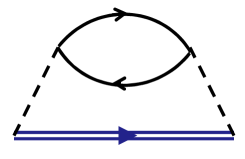
Figure 1: Feynman diagram for TLS self-energy when the bath is in the normal phase. Double blue line represents the TLS Green function, dashed lines the TLS electron-bath interaction, and solid black lines the Green functions of the normal-state bath particles.

In the normal state of the bath, we assume that the bosons are non-interacting with a kinetic energy $E_{\textbf{p}}=|\textbf{p}|^{2}/2m\equiv p^{2}/2m$ and chemical potential $\mu$. To lowest order in the TLS-bath interaction, the self-energy diagram is shown in Fig. 1. Detailed calculation of the self-energy is presented in the Appendix C. The result reads

$$\hat{\Sigma}^{R}(\omega) = \sum_{\textbf{k},\textbf{p}}\left[\hat{M}_{\textbf{k}}\hat{A}\hat{M}_{-\textbf{k}}\frac{(1-n_{\Omega})[n_{B}(\xi_{\textbf{p}})-n_{B}(\xi_{\textbf{p}+\textbf{k}})]+n_{B}(\xi_{\textbf{p}+\textbf{k}})[1+n_{B}(\xi_{\textbf{p}})]}{\omega-\Omega+E_{\textbf{p}}-E_{\textbf{p}+\textbf{k}}+i\delta}\right.$$ (38)

$$\left.+\hat{M}_{\textbf{k}}\hat{B}\hat{M}_{-\textbf{k}}\frac{(1-n_{-\Omega})[n_{B}(\xi_{\textbf{p}})-n_{B}(\xi_{\textbf{p}+\textbf{k}})]+n_{B}(\xi_{\textbf{p}+\textbf{k}})[1+n_{B}(\xi_{\textbf{p}})]}{\omega+\Omega+E_{\textbf{p}}-E_{\textbf{p}+\textbf{k}}+i\delta}\right],$$

where $\xi_{\textbf{p}}=E_{\textbf{p}}-\mu$ is the energy of the bath bosons rendered from the chemical potential, $n_{B}(\xi)=[\exp(\xi/T)-1]^{-1}$ is the Bose distribution function, and

$$\hat{M}_{\textbf{k}}=\left(\begin{array}[]{cc}g_{1}\int d\textbf{r}e^{i\textbf{kr}}|\psi_{1}(\textbf{r})|^{2}&0\\ 0&g_{2}\int d\textbf{r}e^{i\textbf{kr}}|\psi_{2}(\textbf{r})|^{2}\\ \end{array}\right),$$ (39)

Taking the imaginary part of Eq. (38), integrating over the angle between k and p, and substituting the resulting expression into Eqs. (36)-(37) we find the relaxation times

$$\frac{1}{2\tau_{u}} = \frac{m}{(2\pi)^{2}}\int_{0}^{\infty}dk\left[\int_{k/2}^{\infty}\frac{\alpha_{k}f_{\Omega}^{u}(p)pdp}{\sqrt{p^{2}-(k/2)^{2}}}\right.$$

$$\left.+\int_{|{k}/2-{2m\Omega}/{k}|}^{\infty}\frac{\beta_{k}f_{-\Omega}^{u}(p)pdp}{\sqrt{p^{2}-\left({k}/{2}-{2m\Omega}/{k}\right)^{2}}}\right],$$

$$\frac{1}{2\tau_{l}} = \frac{m}{(2\pi)^{2}}\int_{0}^{\infty}dk\left[\int_{k/2}^{\infty}\frac{\gamma_{k}f_{-\Omega}^{l}(p)pdp}{\sqrt{p^{2}-(k/2)^{2}}}\right.$$

$$\left.+\int_{|{k}/{2}+{2m\Omega}/{k}|}^{\infty}\frac{\beta_{k}f_{\Omega}^{l}(p)pdp}{\sqrt{p^{2}-\left({k}/{2}+{2m\Omega}/{k}\right)^{2}}}\right].$$

Here we have introduced the coefficients

$$\alpha_{k}=\textmd{Tr}\left(\hat{A}\hat{M}_{\textbf{k}}\hat{A}\hat{M}^{\ast}_{\textbf{k}}\right)=\left|g_{1}(M_{\textbf{k}})_{11}u^{2}+g_{2}(M_{\textbf{k}})_{22}v^{2}\right|^{2},$$

$$\beta_{k}=\textmd{Tr}\left(\hat{B}\hat{M}_{\textbf{k}}\hat{A}\hat{M}^{\ast}_{\textbf{k}}\right)=|uv|^{2}\left|g_{1}(M_{\textbf{k}})_{11}-g_{2}(M_{\textbf{k}})_{22}\right|^{2},$$

$$\gamma_{k}=\textmd{Tr}\left(\hat{B}\hat{M}_{\textbf{k}}\hat{B}\hat{M}^{\ast}_{\textbf{k}}\right)=\left|g_{1}(M_{\textbf{k}})_{11}v^{2}+g_{2}(M_{\textbf{k}})_{22}u^{2}\right|^{2},$$ (42)

and

$$f^{u}_{\Omega}(p) = f^{l}_{-\Omega}(p)=n_{B}(\xi_{\textbf{p}})[1+n_{B}(\xi_{\textbf{p}})],$$

$$f^{u}_{-\Omega}(p) = n_{\Omega}[n_{B}(\xi_{\textbf{p}})-n_{B}(\xi_{\textbf{p}}+2\Omega)]$$

$$+n_{B}(\xi_{\textbf{p}}+2\Omega)[1+n_{B}(\xi_{\textbf{p}})],$$

$$f^{l}_{\Omega}(p) = \theta(E_{\textbf{p}}-2\Omega)\left\{n_{-\Omega}[n_{B}(\xi_{\textbf{p}})-n_{B}(\xi_{\textbf{p}}-2\Omega)]\right.$$ (43)

$$\left.+n_{B}(\xi_{\textbf{p}}-2\Omega)[1+n_{B}(\xi_{\textbf{p}})]\right\},$$

II.2.2 Bath in the condensed state

We now consider the bath to be in the Bose condensed phase and obtain the TLS self-energy. The elementary excitations of the Bose-condensed system are Bogoliubov quasi-particles. An explicit form of the dispersion law of Bogoliubov excitations depends on the model used to describe the system of interacting bosons. In the case of small particle density an appropriate theoretical model is the Bogoluibov model of weakly-interacting Bose gas. In the framework of this model, the dispersion law of elementary excitations has the form of $\epsilon_{\textbf{p}}=\sqrt{E_{\textbf{p}}\left(E_{\textbf{p}}+2g_{0}n_{c}\right)}$, where $n_{c}$ is particle density in the condensate and $g_{0}$ the strength of inter-particle interaction. In the low-energy, long-wavelength limit $E_{\textbf{p}}\ll 2g_{0}n_{c}$ the elementary excitations comprise sound quanta, with a dispersion $\epsilon_{\textbf{p}}\approx sp$ where $s=\sqrt{g_{0}n_{c}/m}$ is the sound velocity. In the Bose-condensed state, most of the particles are in the condensate but there are also noncondensate particles, due to both interaction and finite temperature effects (thermal-excited particles). All three fractions of particles contribute to relaxation times of TLS. We consider the quantum limit $T\ll sp$ when thermal excitations are not important and the theory can be developed for $T=0$. In the present dilute boson gas limit, the density of the noncondensate particles is small, and one can neglect the interaction term due to fluctuations of the condensate density and the noncondensate density. Thus, the contribution to relaxation times due to the condensate and noncondensate particles can be calculated independently.

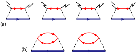
Figure 2: Feynman diagrams for TLS self-energy when the bath is in the BEC phase. Type (a) describes the condensate particles contribution, $\bar{\Sigma}^{c}$, and (b) is due to the non-condensate particles, $\bar{\Sigma}^{n}$. Double blue line represents the TLS Green function and dashed lines the TLS electron-bath interaction. Red lines denote the normal or anomalous Green functions of the non-condensate particles, and the zigzag lines stand for $\sqrt{n_{c}}$ corresponding to the condensate particles.

The self-energy diagrams in the lowest order with respect to the TLS-bath coupling are depicted in Fig. 2. Fig. 2(a) corresponds to the contribution to the self-energy from the condensate particles and describes virtual processes in which a condensate particle is scattered by a TLS electron through an intermediate non-condensate state. Fig. 2(b) corresponds to the contribution from the non-condensate particles and describes polarization of the non-condensate particles induced by the TLS electrons. These self-energy contributions due to condensate particles $\hat{\Sigma}^{cR}$ and non-condensate $\hat{\Sigma}^{nR}$ particles have the following form (see Appendix C)

$$\hat{\Sigma}^{cR}(\omega) = \frac{n_{c}}{2ms}\sum_{\textbf{k}}k\left[\hat{M}_{\textbf{k}}\hat{A}\hat{M}_{-\textbf{k}}\left(\frac{1-n_{\Omega}}{\omega-\Omega-\epsilon_{\textbf{k}}+i\delta}+\frac{n_{\Omega}}{\omega-\Omega+\epsilon_{\textbf{k}}+i\delta}\right)\right.$$ (44)

$$\left.+\hat{M}_{\textbf{k}}\hat{B}\hat{M}_{-\textbf{k}}\left(\frac{1-n_{-\Omega}}{\omega+\Omega-\epsilon_{\textbf{k}}+i\delta}+\frac{n_{-\Omega}}{\omega+\Omega+\epsilon_{\textbf{k}}+i\delta}\right)\right],$$

$$\hat{\Sigma}^{nR}(\omega) = \frac{(ms^{2})^{2}}{2}\sum_{\textbf{k},\textbf{p}}\left[\frac{\hat{M}_{\textbf{k}}\hat{A}\hat{M}_{-\textbf{k}}}{\epsilon_{\textbf{p}}\epsilon_{\textbf{p}+\textbf{k}}}\left(\frac{1-n_{\Omega}}{\omega-\Omega-\epsilon_{\textbf{p}}-\epsilon_{\textbf{p}+\textbf{k}}+i\delta}+\frac{n_{\Omega}}{\omega-\Omega+\epsilon_{\textbf{p}}+\epsilon_{\textbf{p}+\textbf{k}}+i\delta}\right)\right.$$ (45)

$$\left.+\frac{\hat{M}_{\textbf{k}}\hat{B}\hat{M}_{-\textbf{k}}}{\epsilon_{\textbf{p}}\epsilon_{\textbf{p}+\textbf{k}}}\left(\frac{1-n_{-\Omega}}{\omega+\Omega-\epsilon_{\textbf{p}}-\epsilon_{\textbf{p}+\textbf{k}}+i\delta}+\frac{n_{-\Omega}}{\omega+\Omega+\epsilon_{\textbf{p}}+\epsilon_{\textbf{p}+\textbf{k}}+i\delta}\right)\right].$$

Similar steps leading to Eqs. (II.2.1)-(II.2.1) yields

$$\frac{1}{2\tau^{c}_{u}} = \frac{1}{2\tau^{c}_{l}}=n_{\Omega}\frac{\pi n_{c}}{2ms}\sum_{k}k\beta_{k}\delta(-2\Omega+\epsilon_{\textbf{k}}),$$ (46)

$$\frac{1}{2\tau^{n}_{u}} = \frac{1}{2\tau^{n}_{l}}$$

$$= n_{\Omega}\frac{\pi(ms^{2})^{2}}{2}\sum_{\textbf{k},\textbf{p}}\frac{\beta_{k}}{\epsilon_{\textbf{p}}\epsilon_{\textbf{p}+\textbf{k}}}\delta(2\Omega-\epsilon_{\textbf{p}}-\epsilon_{\textbf{p}+\textbf{k}}).$$

Explicit expressions for relaxation times depend on the shape of the wave functions of the TLS upper and lower states through the matrix elements Eq. (39). In the next section we propose and analyze an experimental setup in which explicit expressions of the relaxation time can be obtained.

III Application to coupled QD-dipolar exciton bath

Applying our theory developed in the previous sections, we consider the nanostructure depicted in Fig. 3. A double quantum well (DQW) with closely separated electron-doped and hole doped wells realizes a 2D gas of indirect excitons (also called dipolar excitons). A self-assembled QD is positioned above the DQW and is irradiated with a frequency close to the lowest exciton energy of the QD. In the electron-hole representation of the QD, the lower quantum state describes the unexcited QD state (i.e. vaccum) $|vac\rangle$, while the lowest excited QD state describes the state $|eh\rangle$ of an excited electron-hole pair upon irradiation QD_TLS1 ; QD_TLS2 ; QD_TLS3 . With a shift in energy that does not affect the system’s dynamics, we can assume that these two QD states correspond exactly to the lower and upper TLS levels in Eq. (1) with $\Delta=(E_{e}+E_{h})/2$, where $E_{e,h}$ are the lowest energies of electrons and holes in the QD (corresponding to the energies at the conduction and valence band edges), and $\lambda$ represents the dipole matrix element weighted by the electron-hole pair envelope wave function integrated over all space.

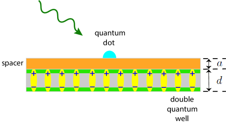
Figure 3: Schematic of the coupled QD-dipolar excitons system. The quantum dot is positioned through a dielectric spacer on top of a double quantum well that hosts the dipolar exciton gas.

Let us discuss the exciton gas model we use for our calculations. The indirect excitons have a dipole moment p in the out-of-plane direction of the DQW. The excitons are modeled as rigid dipole molecules that are free to move on the DQW plane as described by the center-of-mass motion of the dipoles, a valid assumption as long as the dipole’s internal degrees of freedom are not excited. The exciton density $n_{\mathrm{ex}}$ is assumed to be small so that $n_{\mathrm{ex}}a_{B}^{2}\ll 1$, where $a_{B}$ is an exciton Bohr radius. For simplicity, we assume that there is no particle tunneling between the QD and the DQW so that the exchange contribution to the interaction potential is negligible. This can be guaranteed using a large-band gap dielectric spacer as a substrate between the QD and the DQW. The direct contribution to the interaction potential between the electron-hole pair in the QD and the excitons in the DQW is given by

$$U=\int d\textbf{r}\int d\textbf{r}^{\prime}\left(|\chi_{h}(\textbf{r})|^{2}-|\chi_{e}(\textbf{r})|^{2}\right)|\varphi(\textbf{r}^{\prime})|^{2}u(\textbf{r}-\textbf{r}^{\prime}),$$ (48)

$$u(\textbf{r}-\textbf{r}^{\prime})=\frac{e^{2}}{\varepsilon\sqrt{(\textbf{r}-\textbf{r}^{\prime})^{2}+a^{2}}}-\frac{e^{2}}{\varepsilon\sqrt{(\textbf{r}-\textbf{r}^{\prime})^{2}+(a+d)^{2}}},$$ (49)

where $\chi_{e,h}(\textbf{r})$ are the electron (e) and hole (h) wave functions in the QD, $\varphi(\textbf{r})$ is the QW exciton center-of-mass wave function, $\varepsilon$ is an effective dielectric constant taking account of the dielectric environment of the spacer and the DQW, $a$ and $d$ are the distance of the QD to the DQW surface and the separation between the positive charges and negative charges of the dipole layer (see Fig. 3). The Fourier transform of $u(\textbf{r})$ yields

$$u(\textbf{k})=\frac{2\pi e^{2}}{\varepsilon k}\left(1-e^{-kd}\right)e^{-ka}.$$ (50)

Typical values of the wave vector $k$ here are determined by the bath excitons of DQW. At temperatures above the condensation temperature $T>T_{c}$, the bath in the normal state, the DQW exciton energy is of the order of $T$ and thus the wave vector $k\sim p_{T}=\sqrt{2mT}$, where $m$ is the exciton mass. At $T=0$, the bath is in the condensed phase, the typical value of the bath excitation momentum is of the order of $p\leq ms$. Hereafter we assume the distance of the QD from the DQW as well as the inter-well distance in the DQW to be sufficiently small so that $p_{T}a,p_{T}d\ll 1$ and $(ms)a,(ms)d\ll 1$. This allows us to simplify the expression Eq. (50) assuming that $kd,ka\ll 1$. Thus we have

$$u(\textbf{k})\equiv U_{0}=\frac{2\pi e^{2}d}{\varepsilon},\,\,\,u(\textbf{r})=U_{0}\delta(\textbf{r}).$$ (51)

Under this approximation the interaction Eq. (48) becomes contact-like,

$$U=U_{0}\int d\textbf{r}\left(|\chi_{h}(\textbf{r})|^{2}-|\chi_{e}(\textbf{r})|^{2}\right)|\varphi(\textbf{r})|^{2}.$$ (52)

In our coupled QD-exciton gas system, since the lower level is the vacuum, we have in Eqs.(31) and (32) that the coupling constants $g_{1}=U_{0},\,\,g_{2}=0$ and their respective matrix elements $W_{11}=U,\,\,W_{22}=0$. The QD is described by a two-dimensional system of electrons and holes confined by a parabolic potential. For strongly confined QDs where the QD size $L$ is small compared to the Bohr radius of the electron-hole pair, the lowest-energy electrons and holes are characterized by the wavefunctions QD_TLS2 $\chi_{i}(\textbf{r})=\exp(-\rho^{2}/2a^{2}_{i})/({a_{i}\sqrt{\pi}})$, where $a_{i}$ is an electron $i=e$ or a hole $i=h$ characteristic length determined by the QD confinement potential. Using these wavefunctions, we find the matrix element $(\hat{M}_{\textbf{k}})_{11}=\mathrm{exp}[{-(ka_{h}/2)^{2}}]-\mathrm{exp}[{-(ka_{e}/2)^{2}}]$.

III.1 Relaxation times for normal-state bath

With $ka_{i}\ll 1$, we perform the integration over $k$ in Eqs. (II.2.1)-(II.2.1) and obtain the following expressions for the relaxation times

$$\frac{1}{2\tau_{u}} = \frac{m\alpha_{0}}{(2\pi)^{2}}\int_{0}^{\infty}F_{+}(p,0)n_{B}(\xi_{\textbf{p}})[1+n_{B}(\xi_{\textbf{p}})]pdp$$ (53)

$$+\frac{m\beta_{0}}{(2\pi)^{2}}\int_{0}^{\infty}F_{+}(p,p_{0})f^{u}_{-\Omega}(p)pdp,$$

$$\frac{1}{2\tau_{l}} = \frac{m\gamma_{0}}{(2\pi)^{2}}\int_{0}^{\infty}F_{-}(p,0)n_{B}(\xi_{\textbf{p}})[1+n_{B}(\xi_{\textbf{p}})]pdp$$ (54)

$$+\frac{m\beta_{0}}{(2\pi)^{2}}\int_{0}^{\infty}F_{-}(p,p_{0})f^{l}_{\Omega}(p)pdp,$$

where $F_{\pm}(p,p_{0})=6\pi(p^{4}\pm p^{2}p_{0}^{2}+p_{0}^{4}/6)\theta(p^{2}\pm p_{0}^{2})$ with $p_{0}^{2}=4m\Omega$, and

$$\alpha_{0} = U_{0}^{2}(a_{h}^{2}-a_{e}^{2})^{2}u^{4}/16,$$

$$\beta_{0} = U_{0}^{2}(a_{h}^{2}-a_{e}^{2})^{2}|uv|^{2}/16,$$

$$\gamma_{0} = U_{0}^{2}(a_{h}^{2}-a_{e}^{2})^{2}v^{4}/16.$$ (55)

To simplify Eqs. (53)-(54) we consider two limiting cases. At large temperatures $T\gg\Omega$ [while still small compared to $\hbar^{2}/(2md^{2})$], we can keep up to the zeroth order in $\Omega/T$ with $F_{\pm}(p,p_{0})\approx 6\pi p^{4}$ and $f^{u}_{-\Omega}(p)\approx f^{l}_{\Omega}(p)\approx n_{B}(\xi_{\textbf{p}})[1+n_{B}(\xi_{\textbf{p}})]$ in Eqs. (53)-(54). The relaxation rates for $\Omega\ll T$ then read

$$\frac{1}{\tau_{u,l}}=\frac{1}{\tau_{T}}\left(1\pm\frac{\varepsilon_{0}}{\Omega}\right)\mathrm{Li}_{2}\left(e^{\mu/T}\right),$$ (56)

where the $+,-$ signs apply for $\tau_{u,l}$ respectively, and

$$\frac{1}{\tau_{T}}=\frac{3U_{0}^{2}m^{4}T^{3}(a_{h}^{2}-a_{e}^{2})^{2}}{4\pi\hbar^{9}},$$ (57)

and $\mathrm{Li}_{2}(x)$ is the polylogarithm function of order $2$. In the opposite limit of low temperatures $T\ll\Omega$, we keep up to the zeroth order in $T/\Omega$. Then the respective first terms in Eqs. (53)-(54) drop out, and we have $f^{u}_{-\Omega}(p)\approx n_{\Omega}n_{B}(\xi_{\textbf{p}})$ and $f^{l}_{\Omega}(p)\approx n_{\Omega}\theta(E_{\textbf{p}}-2\Omega)n_{B}(\xi_{\textbf{p}}-2\Omega)$ in the second terms. The result is

$$\frac{1}{\tau_{u}}=\frac{1}{\tau_{l}}=\frac{1}{\tau_{T}}n_{\Omega}\frac{\pi^{2}}{3}\left(\frac{\lambda}{T}\right)^{2}\frac{\hbar^{2}n_{\mathrm{ex}}}{mT},$$ (58)

where $n_{\mathrm{ex}}$ is the exciton density in the bath. We have restored $\hbar$ in the expressions for the relaxation rates here and in the following section.

III.2 Relaxation times for Bose-condensed bath

Straightforward but cumbersome integration in Eqs. (46)-(II.2.2) results in the following expressions for relaxation times due to the condensate and non-condensate particles in the bath

$$\frac{1}{2\tau^{c}_{u}}=\frac{1}{2\tau^{c}_{l}}=n_{\Omega}\frac{|\lambda|^{2}n_{c}U_{0}^{2}}{4\hbar^{3}ms^{4}}\left[e^{-(\Omega a_{h}/s)^{2}}-e^{-(\Omega a_{e}/s)^{2}}\right]^{2},$$ (59)

and

$$\frac{1}{2\tau^{n}_{u}}=\frac{1}{2\tau^{n}_{l}}=n_{\Omega}\frac{|\lambda|^{2}m^{2}sU_{0}^{2}}{16\pi^{2}\hbar^{4}\Omega^{2}}$$ (60)

$$\times\left[\frac{F(\sqrt{2}\Omega a_{h}/s)}{a_{h}\sqrt{2}}+\frac{F(\sqrt{2}\Omega a_{e}/s)}{a_{e}\sqrt{2}}-2\frac{F(\sqrt{a_{h}^{2}+a_{e}^{2}}\Omega/s)}{\sqrt{a_{h}^{2}+a_{e}^{2}}}\right],$$

where $F(x)$ is the Dawson integral

$$F(x)=e^{-x^{2}}\int_{0}^{x}e^{t^{2}}dt.$$

IV Discussion

Simple analysis of Rabi oscillations given above accounting for the finite values of relaxation times yields

$$|\langle\psi_{2}^{+}(0)\psi_{1}(t)\rangle|^{2} = \frac{|\lambda|^{2}}{2\Omega^{2}}\left(1-\cos\Omega t\right)e^{-{t}\left({1}/{2\tau_{u}}+{1}/{2\tau_{l}}\right)}$$ (61)

$$+\frac{|\lambda|^{2}}{4\Omega^{2}}\left(e^{-{t}/{2\tau_{u}}}-e^{-{t}/{2\tau_{l}}}\right)^{2}.$$

We focus our discussion on the low temperature regime $T\ll\Omega$. First we note that the relaxation rates for the upper and lower levels coincide both in the normal phase [Eq. (58)] and in the Bose-condensed phase [Eqs. (59)-(60)]. With relaxation times for the upper and lower levels being equal, Eq. (61) is simplified to

$$|\langle\psi_{2}^{+}(0)\psi_{1}(t)\rangle|^{2}=\frac{|\lambda|^{2}}{2\Omega^{2}}\left(1-\cos\Omega t\right)e^{-t/\tau},$$

where $1/\tau=1/\tau_{u}=1/\tau_{l}$, with $1/\tau$ given by Eq. (58) in the normal phase and by $1/\tau^{c}+1/\tau^{n}$ from Eqs. (59)-(60) in the BEC phase. Secondly, the relaxation rates are all proportional to the distribution function $n_{\Omega}$ of the dressed quasiparticle states given in Eq. (28). Since $n_{\Omega}=1$ only if the upper dressed quasiparticle state $+\Omega$ is occupied and vanishes otherwise, finite relaxation of the TLS Rabi oscillations occurs only when the pump field frequency exceeds the TLS energy level difference $\omega\geq 2\Delta$ Remark1 . In our following discussion, therefore, we focus on the regime $\omega\geq 2\Delta$. In the normal phase, we note that the low-temperature relaxation rates Eq. (58) are independent of the driving frequency and increases monotonically with the TLS-light coupling as $\lambda^{2}$. In the BEC phase, we find that the relaxation rates Eqs. (59)-(60) exhibit strong non-monotonic dependence on the driving frequency through the Rabi frequency and the TLS-light coupling.

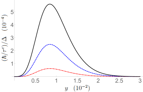
Figure 4: Relaxation rate $\hbar/\tau^{c}$ due to condensate particles (normalized by $\Delta$) versus frequency detuning $y$. Red (dot-dashed), blue (dashed) and black (solid) lines correspond to $\lambda=0.1\,\mathrm{meV}$, $0.2\,\mathrm{meV}$ and $0.3\,\mathrm{meV}$ respectively.

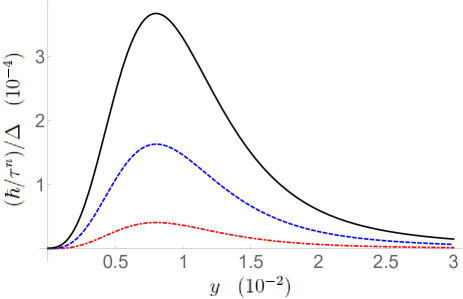
Figure 5: Relaxation rate $\hbar/\tau^{n}$ due to non-condensate particles (normalized by $\Delta$) versus frequency detuning $y$. Red (dot-dashed), blue (dashed) and black (solid) lines correspond to $\lambda=0.1\,\mathrm{meV}$, $0.2\,\mathrm{meV}$ and $0.3\,\mathrm{meV}$ respectively.

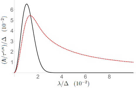
Figure 6: Relaxation rates due to condensate and non-condensate particles versus TLS-light coupling $\lambda/\Delta$ at frequency detuning $y=0.01$. Solid (black) line corresponds to $\hbar/\tau^{c}$ and dashed (red) line to $\hbar/\tau^{n}$, respectively.

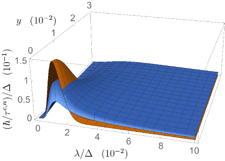
Figure 7: Three-dimensional plot of relaxation rates $\hbar/\tau^{c}$ and $\hbar/\tau^{n}$ as a function of TLS-light coupling $\lambda/\Delta$ and frequency detuning $y$. Grey (red) surface corresponds to $\hbar/\tau^{c}$ and black (blue) surface to $\hbar/\tau^{n}$, respectively.

Below, we proceed to analyze the numerical dependence of the relaxation rates on the driving frequency and TLS-light coupling in the BEC phase. For the TLS, we take the following parameters $\Delta=500\,\mathrm{meV}$, $m_{e}=0.067\,m_{0}$ and $m_{h}=0.45\,m_{0}$ ($m_{0}$ is the electron mass) typical for GaAs-based QDs GaAs_QD1 ; GaAs_QD2 ; GaAs_QD3 . The characteristic lengths of the hole and the electron wavefunctions are taken as $a_{h}=2\,\mathrm{nm}$ and $a_{e}\approx a_{h}\sqrt{m_{h}/m_{e}}=2.23a_{h}$. With the dipole matrix element of the QD $\sim 10\,-\,100\,\mathrm{Debye}$ ($1\,\mathrm{Debye}=3.3\times 10^{-30}\,\mathrm{Cm}$) and optical field strength $0.1\,-\,10\,\mathrm{MVm^{-1}}$, the TLS-light coupling constant takes the range of values $\lambda\sim 0.1\,-\,10\,\mathrm{meV}$. For the dipolar exciton gas, we take $d=10\,\mathrm{nm}$, $n_{c}=10^{10}\,\mathrm{cm}^{-2}$, $\varepsilon=12.5$ and $m=m_{e}+m_{h}=0.517\,m_{0}$ typical for GaAs DQW structures. To provide an estimate for the inter-particle interaction $g_{0}$, we assume a simple point-charge treatment of the dipolar excitons, and the exciton-exciton interaction potential takes the form Zimmermann $g(r)=(2e^{2}/\varepsilon)(1/r-1/\sqrt{r^{2}+d^{2}})$. Fourier transform of $g(r)$ then gives $g(k)=(4\pi e^{2}/\varepsilon k)[1-\mathrm{exp}(-kd)]$ and the coupling constant $g_{0}\equiv g(k=0)=4\pi e^{2}d/\varepsilon$. The Bogoliubov speed of sound $s$ is thus also fixed from $s=\sqrt{g_{0}n_{c}/m}$.

For convenience, we display the frequency $\omega$ in terms of the dimensionless frequency detuning $y=(\omega-2\Delta)/(2\Delta)$. Figs. 4-5 show the relaxation rates $\hbar/\tau^{c}$ and $\hbar/\tau^{n}$ as a function of $y$ for relatively small values of $\lambda\sim 0.1\,\mathrm{meV}$. We find that both relaxation rates behave non-monotonically as a function of detuning, reaching maximum values at $y\sim 0.01$ and then becoming exponentially suppressed at larger values of $y$. $\hbar/\tau^{c}$ is more strongly suppressed than $\hbar/\tau^{n}$. Secondly, we observe that, for the present values of $\lambda\sim 0.1\,\mathrm{meV}$, the condensate and non-condensate fractions contribute to the relaxation rate by the same order of magnitude, with $\hbar/\tau^{c}$ exceeding $\hbar/\tau^{n}$. This trend is maintained until $\lambda$ reaches $\sim 1\%$ of $\Delta$ (corresponding to $5\,\mathrm{meV}$), when $\hbar/\tau^{c}$ starts to drop signifcantly faster than $\hbar/\tau^{n}$. Fig. 6 shows both quantities plotted versus $\lambda/\Delta$ at a frequency detuning $y=0.01$, from which we observe that $\hbar/\tau^{c}$ decreases much more abruptly than $\hbar/\tau^{n}$. When $\lambda$ is increased beyond $\sim 0.02\Delta$, it is seen that $\hbar/\tau^{n}$ now overtakes $\hbar/\tau^{c}$. For $\lambda$ values beyond $0.03\Delta$, $\hbar/\tau^{c}$ has dropped essentially to zero and the non-condensate fraction constitutes the dominant contribution to relaxation.

Although the relaxation rates vanish expectedly when $\lambda=0$, they do not vanish at zero frequency detuning $y=0$, as one might conclude by inspecting Figs. 4-5. To examine more fully the behavior of $\hbar/\tau^{c}$ and $\hbar/\tau^{n}$, we plot them in Fig. 7 in the full range of $\lambda$ and $y$. At $y=0$, both relaxation rates become small only when $\lambda\ll\Delta$; in addition $\hbar/\tau^{c}$ also become small when $\lambda\gtrsim 0.03\Delta$. Around $\lambda\sim 0.01\Delta$, both relaxation rates as a function of $y$ reach maximum at $y=0$.

Conventionally, the BEC phase transition of a dipolar exciton gas is detected using optical spectroscopy. In the BEC phase, the excitons or exciton-polaritons are described by a single coherent wave function and emit light coherently. The resulting luminescence peak becomes much narrower in comparison with that in the normal phase, signaling formation of the condensate state. Another way to detect the BEC phase transition has been theoretically suggested recently 10_RefKovalevChaplikJETP2016 ; 10_1RefKovalevChaplikJETPLetters2016 . BEC phase transition strongly influences the non-equilibrium properties of a dipolar exciton gas driven by an external surface acoustic waves (SAW). Under phase transition, the SAW attenuation effect and the SAW-exciton drag current become strongly modified, allowing one to detect the BEC phase transition using acoustic spectroscopy. On top of the foregoing, our findings in principle provide a new strategy to detect the BEC phase transition of the dipolar exciton gas. While the QD’s relaxation rate displays only a monotonic linear dependence on the light intensity when the exciton gas is in the normal phase, it becomes strongly non-monotonic as a function of both the pump field’s frequency and intensity once the exciton gas is in the BEC phase. Thus, by monitoring the Rabi oscillation dynamics of the QD, the normal and condensed phases of the exciton gas can be distinguished by the dependence of the relaxation rate on the frequency and intensity of the driving field.

V Conclusion

To conclude, we have developed a theory for the relaxation of optically pumped two-level systems coupled to a bosonic bath using the nonequilibrium Keldysh technique and the diagrammatic perturbation theory. To elucidate the effects of bath phase transition, we have considered the cases when the bosonic bath is in the normal state and in the Bose-condensed state. We then apply our theory to study the scenario of an illuminated quantum dot coupled to a dipolar exciton gas. The condensate and non-condensate fractions of the bath particles contribute to the relaxation rate by variable proportions depending on the value of pump field amplitude. When the pump field is weak, both fractions contribute by about the same order of magnitude; while for strong pump field, the non-condensate fraction becomes the dominant contribution. Our findings also show that the phase transition of the dipolar exciton gas to the BEC regime results in a strong dependence of the relaxation rate on the optical pump field. The relaxation rate then exhibits a strong non-monotonic behavior, reaching a maximum and then becoming exponentially suppressed as a function of both the pump field’s frequency and amplitude. Such a non-monotonic dependence could in principle serve as a smoking gun for detecting BEC phase transition of the coupled dipolar exciton gas. Finally, we point out that despite our focus on dipolar exciton gas in this work, the theory we have developed is also applicable to other types of Bose gas, such as 2D exciton-polaritons 10_7Deng2010 , magnons 10_8Pokrovskii2013 and cold atoms 10_9Pethick2002 .

VI Acknowledgments

V.M.K. acknowledges the support from RFBR grant $\#16-02-00565a$. W.K. acknowledges the support by a startup fund from the University of Alabama.

VII Appendix

VII.1 Non-Equilibrium Green’s Functions

Because of the time-dependent perturbation from light, we employ the Keldysh formalism to calculate the Green’s function and distribution function of the system. Following established routes in non-equilibrium Green’s function formalism, the left-multiplied and right-mulitplied Dyson equations for the contour-ordered Green’s function ${G}^{c}$ are

$$G_{0}^{-1}{G}^{c} = 1+{\Sigma}^{c}{G}^{c},$$ (62)

$${G}^{c}G_{0}^{-1} = 1+{G}^{c}{\Sigma}^{c}.$$ (63)

We are interested in the Green’s function of the TLS under irradiation, therefore the self-energy ${\Sigma}$ due to interaction with the bath is set to zero. In the rotating frame, we already find

$$\hat{G}_{0}^{-1}(t,t^{\prime})=\left(\begin{array}[]{cc}i\partial_{t}-\left(\Delta-\frac{\omega}{2}\right)&-\lambda\\ -\lambda^{\ast}&i\partial_{t}+\left(\Delta-\frac{\omega}{2}\right)\\ \end{array}\right).$$ (66)

First we derive the retarded Green’s function. Applying Langreth’s rules 14_Jauhobook to the two equations in Eq. (63) and summing them together, we have $\hat{G}_{0}^{-1}\hat{G}^{R}+\hat{G}^{R}\hat{G}_{0}^{-1}=2\delta(t-t^{\prime})$,

$$\left(i\frac{\partial\hat{G}^{R}}{\partial t}-\hat{H}_{0}\hat{G}^{R}\right)+\left(-i\frac{\partial\hat{G}^{R}}{\partial t^{\prime}}-\hat{G}^{R}\hat{H}_{0}\right)=2\delta(t-t^{\prime}).$$

(67)

We transform the time variables $t,t^{\prime}$, into the Wigner coordinates with the average time $T=(t+t^{\prime})/2$ and relative time $\tau=t-t^{\prime}$. Eq. (67) becomes

$$i2\frac{\partial\hat{G}^{R}}{\partial\tau}-\left\{\hat{H}_{0},\hat{G}^{R}\right\}=2\delta(\tau).$$ (68)

Performing Fourier transformation with respect to $\tau$ gives

$$2\varepsilon\hat{G}^{R}-\left\{\hat{H}_{0},\hat{G}^{R}\right\}=2.$$ (69)

Solving this matrix equation yields the retarded Green’s function in Eq. (13):

$$\hat{G}^{R}(\varepsilon,T) = \frac{1}{2\Omega}\left(\begin{array}[]{cc}\varepsilon+\varepsilon_{0}&\lambda\\ \lambda^{\ast}&\varepsilon-\varepsilon_{0}\\ \end{array}\right)$$

$$\times\left[\frac{1}{\varepsilon-\Omega+i\delta}-\frac{1}{\varepsilon+\Omega+i\delta}\right]$$

$$= \hat{A}\frac{1}{\varepsilon-\Omega+i\delta}+\hat{B}\frac{1}{\varepsilon+\Omega+i\delta},$$ (73)

with $\hat{A},\hat{B}$ defined in Eq. (14).

Now from the contour-ordered Dyson’s equations Eq. (63) and applying Langreth’s rule, then subtracting the two equations, we get $G_{0}^{-1}G^{<}-G^{<}G_{0}^{-1}=0$,

$$\left(i\frac{\partial\hat{G}^{<}}{\partial t}-\hat{H}_{0}\hat{G}^{<}\right)-\left(-i\frac{\partial\hat{G}^{<}}{\partial t^{\prime}}-\hat{G}^{<}\hat{H}_{0}\right)=0,$$ (74)

Transforming into the Wigner coordinates, we obtain the kinetic equation

$$i\frac{\partial\hat{G}^{<}}{\partial t}-\left[\hat{H}_{0},\hat{G}^{<}\right]=0$$ (75)

The density matrix $f(t)$ is given by the equal-time Keldysh Green’s function $\hat{f}(t)=-i\hat{G}^{<}(t,t)=-i\hat{G}^{<}(T=t,\tau=0)$, which satisfies

$$\frac{\partial\hat{f}}{\partial T}+i[\hat{H}_{0},\hat{f}]=0.$$ (76)

VII.2 Quasiparticle Lifetimes

We start from Eq. (34) in the main text

$$\hat{G}^{R}=\frac{1}{\Lambda}\left[{\hat{G}_{0}^{R}-\det(\hat{G}_{0}^{R})\sigma_{y}(\hat{\Sigma}^{R})^{\mathrm{T}}\sigma_{y}}\right].$$

From Eqs. (13)-(14) it can be easily evaluated that $\det(\hat{G}_{0}^{R})=1/(\varepsilon^{2}-\Omega^{2}+i\delta)$. Upon substitution of Eq. (13), the first term of Eq. (34) can be written as follows

$$\frac{\hat{G}_{0}^{R}}{\Lambda} = \frac{\hat{A}}{\varepsilon-\Omega-\mathrm{Tr}(\hat{A}\hat{\Sigma}^{R})-\mathrm{Tr}(\hat{B}\hat{\Sigma}^{R})(\varepsilon-\Omega)/(\varepsilon+\Omega)+\det(\hat{\Sigma}^{R})/(\varepsilon+\Omega)}$$ (77)

$$+ \frac{\hat{B}}{\varepsilon+\Omega-\mathrm{Tr}(\hat{A}\hat{\Sigma}^{R})(\varepsilon+\Omega)/(\varepsilon-\Omega)-\mathrm{Tr}(\hat{B}\hat{\Sigma}^{R})+\det(\hat{\Sigma}^{R})/(\varepsilon-\Omega)}.$$

In the vicinity of the poles we have

$$\frac{\hat{G}_{0}^{R}}{\Lambda} \approx \frac{\hat{A}}{\varepsilon-\Omega-\mathrm{Tr}(\hat{A}\hat{\Sigma}^{R})|_{\varepsilon=\Omega}+\det(\hat{\Sigma}^{R})|_{\varepsilon=\Omega}/(2\Omega)}$$

$$+ \frac{\hat{B}}{\varepsilon+\Omega-\mathrm{Tr}(\hat{B}\hat{\Sigma}^{R})|_{\varepsilon=-\Omega}-\det(\hat{\Sigma}^{R})|_{\varepsilon=-\Omega}/(2\Omega)}.$$

Since $\hat{\Sigma}^{R}\sim 1/\tau$ where $\tau$ is the quasiparticle lifetime, $1/\tau\ll\Omega$ is satisfied for our perturbative calculations. We see that the last terms in the denominators above $\det(\hat{\Sigma}^{R})|_{\varepsilon=\pm\Omega}/(2\Omega)\sim(1/\tau)\times 1/(\Omega\tau)$ are a factor of $1/(\Omega\tau)$ smaller than $1/\tau$ and thus can be neglected. Next we consider the second term of Eq. (34), whereupon substituting Eq. (13) becomes

$$\frac{\det(\hat{G}_{0}^{R})\sigma_{y}(\hat{\Sigma}^{R})^{\mathrm{T}}\sigma_{y}}{\Lambda} = \frac{\sigma_{y}(\hat{\Sigma}^{R})^{\mathrm{T}}\sigma_{y}}{\varepsilon^{2}-\Omega^{2}-(\varepsilon+\Omega)\mathrm{Tr}(\hat{A}\hat{\Sigma}^{R})-(\varepsilon-\Omega)\mathrm{Tr}(\hat{B}\hat{\Sigma}^{R})+\det(\hat{\Sigma}^{R})}.$$ (79)

In the vicinity of the upper level where $\varepsilon\approx\Omega$,

$$\frac{\det(\hat{G}_{0}^{R})\sigma_{y}(\hat{\Sigma}^{R})^{\mathrm{T}}\sigma_{y}}{\Lambda}$$

$$\approx \frac{1}{2\Omega}\frac{\sigma_{y}(\hat{\Sigma}^{R})^{\mathrm{T}}\sigma_{y}}{\varepsilon-\Omega-\mathrm{Tr}(\hat{A}\hat{\Sigma}^{R})|_{\varepsilon=\Omega}+\det(\hat{\Sigma}^{R})|_{\varepsilon=\Omega}/(2\Omega)}.$$

We see that the expression in the last line above is a factor of $1/(\Omega\tau)$ smaller than the corresponding $\varepsilon\approx\Omega$ contribution (i.e., the term $\propto\hat{A}$) in Eq. (VII.2), and hence can be neglected. A similar analysis shows that the same is true for the $\varepsilon\approx-\Omega$ contribution in Eq. (79). Therefore we find

$$\hat{G}^{R}(\epsilon) \approx \frac{\hat{A}}{\varepsilon-\Omega-\mathrm{Tr}(\hat{A}\hat{\Sigma}^{R})|_{\varepsilon=\Omega}}$$ (81)

$$+ \frac{\hat{B}}{\varepsilon+\Omega-\mathrm{Tr}(\hat{B}\hat{\Sigma}^{R})|_{\varepsilon=-\Omega}},$$

which gives Eq. (35) with Eqs. (36)-(37) in the main text.

VII.3 TLS Self-Energy

Here we derive the expression for the TLS self-energy. Analytic expression of the diagram depicted in Fig. 1 reads

$$\hat{\Sigma}(t-t^{\prime})=i\int\frac{d\textbf{k}}{(2\pi)^{2}}\hat{M}_{\textbf{k}}\hat{{G}}(t-t^{\prime})\hat{M}_{-\textbf{k}}\Pi(\textbf{k},t-t^{\prime}),$$

$$\Pi(\textbf{k},t-t^{\prime})=i\sum_{\textbf{p}}\mathcal{G}(\textbf{p},t-t^{\prime})\mathcal{G}(\textbf{p}+\textbf{k},t^{\prime}-t),$$ (82)

where times $t,t^{\prime}$ are located on the Keldysh contour, $\Pi$ and $\mathcal{G}$ are the polarization operator and Green’s function of the bath’s particles.

To proceed further, let us first perform an analytic continuation to the real time domain. Using the Langreth’s rules 14_Jauhobook we find

$$\hat{\Sigma}^{<}(\omega) = i\sum_{\textbf{k},\varepsilon}\hat{M}_{\textbf{k}}\hat{{G}}^{<}(\omega-\varepsilon)\hat{M}_{-\textbf{k}}\Pi^{<}(\textbf{k},\varepsilon),$$ (83)

$$\hat{\Sigma}^{R}(\omega) = i\sum_{\textbf{k},\varepsilon}\hat{M}_{\textbf{k}}\left[\hat{{G}}^{<}(\omega-\varepsilon)\Pi^{R}(\textbf{k},\varepsilon)\right.$$ (84)

$$+\hat{{G}}^{R}(\omega-\varepsilon)\Pi^{<}(\textbf{k},\varepsilon)$$

$$\left.+\hat{{G}}^{R}(\omega-\varepsilon)\Pi^{R}(\textbf{k},\varepsilon)\right]\hat{M}_{-\textbf{k}},$$

$$\Pi^{<}(\textbf{k},\omega) = i\sum_{\textbf{p},\varepsilon}\mathcal{G}^{<}(\textbf{p}+\textbf{k},\varepsilon+\omega)\mathcal{G}^{>}(\textbf{p},\varepsilon),$$ (85)

$$\Pi^{R}(\textbf{k},\omega) = i\sum_{\textbf{p},\varepsilon}[\mathcal{G}^{<}(\textbf{p}+\textbf{k},\varepsilon+\omega)\mathcal{G}^{A}(\textbf{p},\varepsilon)$$ (86)

$$+\mathcal{G}^{R}(\textbf{p}+\textbf{k},\varepsilon+\omega)\mathcal{G}^{<}(\textbf{p},\varepsilon)].$$

VII.3.1 TLS self-energy in normal state bath

Lets consider the bath in normal phase state, $T>T_{c}$. In this case the bare Green’s functions of the bath’s particles are

$$\mathcal{G}^{<}(\textbf{k},\varepsilon) = -2\pi in_{B}(\xi_{\textbf{k}})\delta(\varepsilon-E_{\textbf{k}}),$$ (87)

$$\mathcal{G}^{>}(\textbf{k},\varepsilon) = -2\pi i[1+n_{B}(\xi_{\textbf{k}})]\delta(\varepsilon-E_{\textbf{k}}),$$ (88)

$$\mathcal{G}^{R}(\textbf{k},\varepsilon) = \frac{1}{\varepsilon-E_{\textbf{k}}+i\delta},$$ (89)

where $n_{B}(\xi_{\textbf{k}})$ is equilibrium Bose distribution and $E_{\textbf{k}}=k^{2}/2m$ is the energy of the bath’s particles (which corresponds to the kinetic energy of the exciton’s center-of-mass motion for the excitonic bath we consider in Section III. Using these functions we find the following polarization operators

$$\Pi^{<}(\textbf{k},\omega) = -2\pi i\sum_{\textbf{p}}n_{B}(\xi_{\textbf{k}+\textbf{p}})[1+n_{B}(\xi_{\textbf{p}})]$$ (90)

$$\times\delta(\omega+E_{\textbf{p}}-E_{\textbf{p}+\textbf{k}}),$$

$$\Pi^{R}(\textbf{k},\omega) = \sum_{\textbf{p}}\frac{n_{B}(\xi_{\textbf{p}})-n_{B}(\xi_{\textbf{k}+\textbf{p}})}{\omega+E_{\textbf{p}}-E_{\textbf{p}+\textbf{k}}+i\delta}.$$ (91)

Substituting these expressions into Eq. (83), we obtain the self-energy expression Eq. (38).

VII.3.2 TLS self-energy in BEC bath

If the bath is in the Bose-condensed state, the elementary excitations in the Bogoliubov’s theory of weakly-interacting Bose gas have the energy dispersion

$$\epsilon_{\textbf{k}}=\sqrt{\frac{k^{2}}{2m}\left(\frac{k^{2}}{2m}+2ms^{2}\right)},$$ (92)

where $s^{2}=g_{0}n_{c}/m$ is the Bogolubov quasiparticle’s speed of sound, $g_{0}$ is the inter-particle interaction strength, and $n_{c}$ particles density in the condensate. The Green functions are given by

$$\hat{\mathfrak{G}}^{R}(\textbf{k},\varepsilon) = \left(\begin{array}[]{cc}\mathfrak{G}&\mathfrak{F}^{+}\\ \mathfrak{F}&\tilde{\mathfrak{G}}\\ \end{array}\right)^{R}=\frac{1}{(\varepsilon+i\delta)^{2}-\epsilon_{\textbf{k}}^{2}}$$ (98)

$$\times\left(\begin{array}[]{cc}\varepsilon+k^{2}/2m+ms^{2}&-ms^{2}\\ -ms^{2}&-\varepsilon+k^{2}/2m+ms^{2}\\ \end{array}\right),$$

and

$$\hat{\mathfrak{G}}^{<}(\textbf{k},\varepsilon)=n_{B}(\varepsilon)[\hat{\mathfrak{G}}^{R}(\textbf{k},\varepsilon)-\hat{\mathfrak{G}}^{A}(\textbf{k},\varepsilon)]$$ (102)

$$= -\frac{2\pi i}{2\epsilon_{\textbf{k}}}\left(\begin{array}[]{cc}\varepsilon+k^{2}/2m+ms^{2}&-ms^{2}\\ -ms^{2}&-\varepsilon+k^{2}/2m+ms^{2}\\ \end{array}\right)$$

$$\times\left\{n_{B}(\epsilon_{\textbf{k}})\delta(\varepsilon-\epsilon_{\textbf{k}})+[1+n_{B}(\epsilon_{\textbf{k}})]\delta(\varepsilon+\epsilon_{\textbf{k}})\right\},$$

$$\hat{\mathfrak{G}}^{>}(\textbf{k},\varepsilon)=[1+n_{B}(\varepsilon)][\hat{\mathfrak{G}}^{R}(\textbf{k},\varepsilon)-\hat{\mathfrak{G}}^{A}(\textbf{k},\varepsilon)]$$ (106)

$$= -\frac{2\pi i}{2\epsilon_{\textbf{k}}}\left(\begin{array}[]{cc}\varepsilon+k^{2}/2m+ms^{2}&-ms^{2}\\ -ms^{2}&-\varepsilon+k^{2}/2m+ms^{2}\\ \end{array}\right)$$

$$\times\left\{[1+n_{B}(\epsilon_{\textbf{k}})]\delta(\varepsilon-\epsilon_{\textbf{k}})+n_{B}(\epsilon_{\textbf{k}})\delta(\varepsilon+\epsilon_{\textbf{k}})\right\}.$$

The polarization operator has two contributions. The first one comes from the condensate particles and the other one from non-condensate particles, Fig. 1. If the Bose bath is a two-dimensional system, the condensate occurs at zero temperature only. In this case one assumes that $n_{B}(\epsilon_{\textbf{k}})=0$. The contribution $P_{c}(\textbf{k},\omega)$ to the polarization operator from the condensate particles is

$$P^{R}_{c}(\textbf{k},\omega) = n_{c}[\mathfrak{G}^{R}+\mathfrak{F}^{+R}+\mathfrak{F}^{R}+\tilde{\mathfrak{G}}^{R}]$$ (107)

$$= n_{c}\frac{k^{2}/m}{(\omega+i\delta)^{2}-\epsilon_{\textbf{k}}^{2}},$$

$$P^{<}_{c}(\textbf{k},\omega) = n_{c}[\mathfrak{G}^{<}+\mathfrak{F}^{+<}+\mathfrak{F}^{<}+\tilde{\mathfrak{G}}^{<}]$$ (108)

$$= -\pi in_{c}\frac{k^{2}/m}{\epsilon_{\textbf{k}}}\delta(\omega+\epsilon_{\textbf{k}}).$$

Using this functions one finds the condensate contribution to the retarded self-energy, Eq. (44).

Now let us find the contribution to the self-energy from the non-condensate particles. First, we need the retarded and lesser polarization operators. In the regime $ms^{2}\gg k^{2}/2m$ where linear dispersion $\epsilon_{\textbf{k}}=sk$ of the Bogoliubov quasiparticles holds, using Eqs. (98)-(106) we find for the retarded and lesser polarization operators of non-condensate particles

$$P_{n}^{R}(\textbf{k},\omega) = 2i\sum_{\textbf{p},\varepsilon}\left[\mathfrak{F}^{<}(\textbf{p}+\textbf{k},\varepsilon+\omega)\mathfrak{F}^{+A}(\textbf{p},\varepsilon)\right.$$

$$\left.+\mathfrak{F}^{R}(\textbf{p}+\textbf{k},\varepsilon+\omega)\mathfrak{F}^{+<}(\textbf{p},\varepsilon)\right]$$

$$= \frac{(ms^{2})^{2}}{2}\sum_{\textbf{p}}\frac{1}{\epsilon_{\textbf{p}}\epsilon_{\textbf{p}+\textbf{k}}}\left(\frac{1}{\omega-\epsilon_{\textbf{p}}-\epsilon_{\textbf{p}+\textbf{k}}+i\delta}\right.$$

$$\left.-\frac{1}{\omega+\epsilon_{\textbf{p}}+\epsilon_{\textbf{p}+\textbf{k}}+i\delta}\right),$$

$$P_{n}^{<}(\textbf{k},\omega) = 2i\sum_{\textbf{p},\varepsilon}\mathfrak{F}^{<}(\textbf{p}+\textbf{k},\varepsilon+\omega)\mathfrak{F}^{+>}(\textbf{p},\varepsilon)$$

$$= -\pi i(ms^{2})^{2}\sum_{\textbf{p}}\frac{1}{\epsilon_{\textbf{p}}\epsilon_{\textbf{p}+\textbf{k}}}\delta(\omega+\epsilon_{\textbf{p}}+\epsilon_{\textbf{p}+\textbf{k}}).$$

Now the calculation of the non-condensate particles’ contribution to the self-energy of TLS is simple, and we arrive at the expression Eq. (45) of the main text.

References

- (1) L. Mandel and E. Wolf, Optical Coherence and Quantum Optics (Cambridge University Press, 1995).
- (2) L. Allen and J. H. Eberly, Optical Resonance and Two Level Atoms (Dover Publications, 1987).
- (3) L. M. K. Vandersypen and I. L. Chuang, Rev. Mod. Phys. 76, 1037 (2005).
- (4) I. Chiorescu, P. Bertet, K. Semba, Y. Nakamura, C. J. P. M. Harmans, and J. E. Mooij, Nature 431, 159 (2004).
- (5) A. Wallraff, D. I. Schuster, A. Blais, L. Frunzio, R. S. Huang, J. Majer, S. Kumar, S. M. Girvin, and R. J. Schoelkopf, Nature 431, 162 (2004).
- (6) U. Weiss, Quantum dissipative systems, 2nd ed. (World Scientific, 1999).
- (7) A. Shnirman, Y. Makhlin and G. Schn, Physica Scripta 102, 147 (2002).
- (8) A. J. Leggett, S. Chakravarty, A. T. Dorsey, Matthew P. A. Fisher, Anupam Garg, and W. Zwerger, Rev. Mod. Phys. 59, 1 (1987).
- (9) A. J. Ramsay, Semicond. Sci. Technol. 25, 103001 (2010).
- (10) P. Lodahl, S. Mahmoodian, and S. Stobbe, Rev. Mod. Phys. 87, 347 (2015).
- (11) G. Konstantatos, M. Badioli, L. Gaudreau, J. Osmond, M. Bernechea, F. P. Garcia de Arquer, F. Gatti, and F. H. L. Koppens, Nat. Nanotechnol. 7, 363 (2012).
- (12) S. D. Franceschi, L. Kouwenhoven, C. Schönenberger, and W. Wernsdorfer, Nat. Nanotechnol. 5, 703 (2010).
- (13) O. Cotlet, S. Zeytinoglu, M. Sigrist, E. Demler, and A. Imamoglu, Phys. Rev. B 93, 054510 (2016).
- (14) F. P. Laussy, A. V. Kavokin, and I. A. Shelykh, Phys. Rev. Lett. 104, 106402 (2010).
- (15) I. A. Shelykh, T. Taylor, and A. V. Kavokin, Phys. Rev. Lett. 105, 140402 (2010).
- (16) F. P. Laussy, T. Taylor, I. A. Shelykh, and A. V. Kavokin, J. Nanophotonics 6, 064502 (2012).
- (17) M. Matuszewski, T. Taylor, and A. V. Kavokin, Phys. Rev. Lett. 108, 060401 (2012).
- (18) L. V. Butov, Sol. State Comm. 127, 89 (2003).
- (19) L. V. Butov, J. Phys.: Cond. Matt 16, R1577 (2004).
- (20) L. V. Butov, J. Phys.: Cond. Matt. 19, 295202 (2007).
- (21) V. B. Timofeev, A. V. Gorbunov, Phys. Status Solidi C 5, 2379 (2008).
- (22) V. B. Timofeev, A. V. Gorbunov, J. Exp. Theor. Phys. 84 390 (2006).
- (23) E. V. Calman, C. J. Dorow, M. M. Fogler, L. V. Butov, S. Hu, A. Mishchenko, and A. K. Geim, Appl. Phys. Lett. 108, 101901 (2016).
- (24) P. Rivera, J. R. Schaibley, A. M. Jones, J. S. Ross, S. Wu, G. Aivazian, P. Klement, K. Seyler, G. Clark, N. J. Ghimire, J. Yan, D. G. Mandrus, W. Yao, and X. Xu, et al., Nat. Commun. 6, 6242 (2015).
- (25) M. M. Fogler, L. V. Butov, and K. S. Novoselov, Nat. Commun. 5, 4555 (2014).
- (26) F.-C. Wu, F. Xue, and A. H. MacDonald, Phys. Rev. B 92, 165121 (2015).
- (27) O. L. Berman and R. Ya. Kezerashvili, Phys. Rev. B 93, 245410 (2016).
- (28) J. L. Black and P. Fulde, Phys. Rev. Lett. 43, 453 (1979).
- (29) R. S. Christensen, J. Levinsen and G. M. Bruun, Phys. Rev. Lett. 115, 160401 (2015).
- (30) T. K. Melik-Barkhudarov, Sov. Phys. JETP 48, 48 (1978).
- (31) V. Weisskopf and E. Wigner, Z. Phys., 63 54 (1930).
- (32) J. P. Gordon, L. R. Walker, and W. H. Louisell, Phys. Rev. 130, 804 (1963).
- (33) S. T. Beliaev, Sov. Phys. JETP 7, 289 (1958).
- (34) H. Shi and A. Griffin, Phys. Rep. 304, 1 (1998).
- (35) L. P. Pitaevskii and S. Stringari, Bose-Einstein Condensation, International Series of Monographs on Physics (Clarendon Press, Oxford, 2003).
- (36) L. D. Landau and E. M. Lifshitz, Quantum Mechanics, (Pergamon Press, 1965).
- (37) W. Que, Phys. Rev. B 45, 11036 (1992).
- (38) L. Jacak, P. Hawrylak, and A. Wojs, Quantum Dots, NanoScience and Technology (Springer, 2013).
- (39) H. Kamada, H. Gotoh, J. Temmyo, T. Takagahara, and H. Ando, Phys. Rev. Lett. 87 246401 (2001).
- (40) This follows from our assumption of low-temperatures: the relaxation rate in the normal state obtained in the limit of low temperatures is a zero-temperature result, while the relaxation rate in the Bose-condensed phase is obtained for temperatures below the BEC critical temperature (typically a few kelvins) where the Bogoliubov theory at applies. At higher temperatures, the relaxation rates become non-zero when , as indicated by our result Eq. (56).
- (41) Y. Turki-Ben Ali, G. Bastard, R. Bennaceur, Physica E 27, 67 (2005).
- (42) P. Lelong and G. Bastard, Solid State Commun. 98, 819 (1996).
- (43) G. W. Bryant, Phys. Rev. B 37, 8763 (1988).
- (44) C. Schindler and R. Zimmermann, Phys. Rev. B 78, 045313 (2008).
- (45) V. M. Kovalev and A. V. Chaplik, J. Exp. Theor. Phys. 122 499 (2016).
- (46) M. V. Boev, V. M. Kovalev and A. V. Chaplik, J. Exp. Theor. Phys. Lett. 104 204 (2016).
- (47) H. Deng, H. Haug, and Y. Yamamoto, Rev. Mod. Phys. 82, 1489 (2010).
- (48) F. Li, W. M. Saslow, V. L. Pokrovsky, Scientific Reports, 3, 1372 (2013).
- (49) C. J. Pethick and H. Smith, Bose-Einstein Condensation in Dilute Gases, 2nd ed. (Cambridge University Press, 2002).
- (50) H. Haug and A. P. Jauho, Quantum Kinetics in Transport and Optics of Semiconductors, 2nd ed. (Springer-Verlag, 2008).