On a combinatorial curvature for surfaces with inversive distance circle packing metrics

Abstract

In this paper, we introduce a new combinatorial curvature on triangulated surfaces with inversive distance circle packing metrics. Then we prove that this combinatorial curvature has global rigidity. To study the Yamabe problem of the new curvature, we introduce a combinatorial Ricci flow, along which the curvature evolves almost in the same way as that of scalar curvature along the surface Ricci flow obtained by Hamilton [21]. Then we study the long time behavior of the combinatorial Ricci flow and obtain that the existence of a constant curvature metric is equivalent to the convergence of the flow on triangulated surfaces with nonpositive Euler number. We further generalize the combinatorial curvature to $\alpha$-curvature and prove that it is also globally rigid, which is in fact a generalized Bower-Stephenson conjecture [6]. We also use the combinatorial Ricci flow to study the corresponding $\alpha$-Yamabe problem.

Mathematics Subject Classification (2010). 52C25, 52C26, 53C44.

1 Introduction

This is a continuation of our work on combinatorial curvature in [17]. This paper generalizes our results in [17] to triangulated surfaces with inversive distance circle packing metrics. Circle packing is a powerful tool in the study of differential geometry and geometric topology and there are lots of research on this topic. In his work on constructing hyperbolic structure on 3-manifolds, Thurston ([28], Chapter 13) introduced the notion of Euclidean and hyperbolic circle packing metrics on triangulated surfaces with prescribed intersection angles. The requirement of prescribed intersection angles corresponds to the fact that the intersection angle of two circles is invariant under the Möbius transformations. For triangulated surfaces with Thurston’s circle packing metrics, there will be singularities at the vertices. The classical combinatorial Gauss curvature $K_{i}$ is introduced to describe the singularity at the vertex $v_{i}$, which is defined as the angle deficit at $v_{i}$. Thurston’s work generalized Andreev’s work on circle packing metrics on a sphere [1, 2]. Andreev and Thurston’s work together gave a complete characterization of the space of the classical combinatorial Gauss curvature. As a corollary, they got the combinatorial-topological obstacle for the existence of a constant curvature circle packing metric, which could be written as combinatorial-topological inequalities. Chow and Luo [7] first introduced a combinatorial Ricci flow, a combinatorial analogue of the smooth surface Ricci flow, for triangulated surfaces with Thurston’s circle packing metrics and got the equivalence between the existence of a constant curvature metric and the convergence of the combinatorial Ricci flow. This work is the cornerstone of applications of combinatorial surface Ricci flow in engineering up to now, see for example [30, 32] and the references therein. Luo [23] once introduced a combinatorial Yamabe flow on triangulated surfaces with piecewise linear metrics to study the corresponding constant curvature problem. The combinatorial surface Ricci flow in [7] and the combinatorial Yamabe flow in [23] are recently written in a unified form in [31]. The first author [10, 11] introduced a combinatorial Calabi flow on triangulated surfaces with Thurston’s Euclidean circle packing metrics and proved the equivalence between the existence of constant circle packing metric and the convergence of the combinatorial Calabi flow. The authors [18] further generalized the combinatorial Calabi flow to hyperbolic circle packing metrics and got similar results.

However, there are some disadvantages for the classical discrete Gauss curvature as stated in [17]. The first is that the classical Euclidean discrete Gauss curvature is invariant under scaling, i.e., $K_{i}(\lambda r)=K_{i}(r)$ for any positive constant $\lambda$. The second is that the classical discrete Gauss curvature tends to zero, not the Gauss curvature of the smooth surface, as triangulated surfaces approximate a smooth surface. Motivated by the two disadvantages, the authors [17] introduced a new combinatorial curvature defined as $R_{i}=\frac{K_{i}}{r_{i}^{2}}$ for triangulated surfaces with Thurston’s Euclidean circle packing metrics. If we take $g_{i}=r_{i}^{2}$ as the analogue of the Riemannian metric, then we have $R_{i}(\lambda g)=\lambda^{-1}R_{i}(g)$, which has the same form as that of the smooth Gauss curvature. Furthermore, there are examples showing that this curvature actually approximates the smooth Gauss curvature on surfaces as the triangulated surfaces approximate a smooth surface [17]. Then we introduce a combinatorial Ricci flow and a combinatorial Calabi flow to study the corresponding Yamabe problem and got a complete characterization of the existence of a constant $R$-curvature circle packing metric using these flows. The results in [17] generalized the previous work of the authors in [16]. The authors then further generalized the curvatures to triangulated surfaces with hyperbolic background geometry [18]. We also consider the $\alpha$-curvature and $\alpha$-flows on low dimensional triangulated manifolds in [17, 19].

Thurston introduced the intersection angle in the definition of circle packing metric as it is invariant under the Möbius transformations. The notion of inversive distance of two circles in a Möbius plane was introduced by H.S.M. Coxeter [8], which generalizes the notion of the intersection angle of two circles. Furthermore, the notion of inversive distance is invariant under the Möbius transformations, as it is actually defined by the cross ratio [4]. Bowers and Stephenson [6] introduced the inversive distance circle packing metric for triangulated surfaces, which generalizes Thurston’s circle packing metric defined using intersection angle. The inversive distance circle packing metric has some applications in medical science, see for example [22]. Bowers and Stephenson [6] once conjectured that the inversive distance circle packings are rigid. This conjecture was proved to be locally right by Guo [20] and then finally proved by Luo [24] in Euclidean and hyperbolic background geometry for nonnegative inversive distance. The local rigidity [20] comes from the convexity of an energy function defined on the admissible space and the global rigidity [24] comes from a convex extension of the energy function to the whole space, the idea of which comes from Bobenko, Pinkall and Springborn [5]. Ma and Schlenker [25] gave a counterexample showing that there is no rigidity for the spherical background geometry and John C. Bowers and Philip L. Bowers [3] recently presented a new construction of their counterexample using only the inversive geometry of the 2-sphere. The combinatorial Ricci flow for triangulated surfaces with inversive distance circle packing metrics was introduced in [30, 31], using the classical combinatorial Gauss curvature. Recently, the first author and Jiang [12, 13]studied the long time behavior of the flow using the extending method and got some interesting results.

In this paper, we generalize our definition of combinatorial curvature in [17] for Thurston’s circle packing metrics to inversive distance circle packing metrics. This curvature was also studied at the same time by the first author and Jiang [14] using the flow introduced by the authors in [19]. Given a weighted triangulated surface $(M,\mathcal{T},I)$ with inversive distance $I_{ij}\geq 0$ for every edge $\{ij\}\in E$, for any function $r:V\rightarrow[0,+\infty)$, the edge length $l_{ij}$ is defined to be

$$l_{ij}=\sqrt{r_{i}^{2}+r_{j}^{2}+2r_{i}r_{j}I_{ij}}$$

for Euclidean background geometry and

$$l_{ij}=\cosh^{-1}\left(\cosh r_{i}\cosh r_{j}+I_{ij}\sinh r_{i}\sinh r_{j}\right)$$

for hyperbolic background geometry. If the lengths $\{l_{ij},l_{jk},l_{ik}\}$ satisfy the triangle inequalities for any face $\triangle ijk$, $r$ is called an inversive distance circle packing metric. Denote

$$\Omega_{ijk}=\{(r_{i},r_{j},r_{k})|l_{ij}<l_{ik}+l_{kj},l_{ik}<l_{ij}+l_{jk},l_{jk}<l_{ji}+l_{ik}\}$$

and

$$\Omega=\cap_{\Delta ijk\in F}\Omega_{ijk}=\{r\in\mathds{R}_{>0}^{N}|l_{ij}<l_{ik}+l_{kj},l_{ik}<l_{ij}+l_{jk},l_{jk}<l_{ji}+l_{ik},\forall\Delta ijk\in F\}.$$

If $r\in\Omega$, the triangulated surface could be obtained by gluing many triangles along their edges coherently and there will be singularities at the vertices. The classical discrete Gauss curvature $K$ is introduced to describe the singularity, which is defined as the angle deficit at a vertex, i.e. $K_{i}=2\pi-\sum_{\triangle ijk\in F}\theta_{i}^{jk}$, where $\theta_{i}^{jk}$ is the inner angle of $\triangle ijk$ at $i$. In this paper, we introduce a new combinatorial curvature, which is defined as

$$R_{i}=\frac{K_{i}}{r_{i}^{2}}$$

for Euclidean background geometry and

$$R_{i}=\frac{K_{i}}{\tanh^{2}\frac{r_{i}}{2}}$$

for hyperbolic background geometry. For this combinatorial curvature, we prove the following main theorem on global rigidity.

Theorem 1.1.

Given a weighted closed triangulated surface $(M,\mathcal{T},I)$ with $I\geq 0$ and $\chi(M)\leq 0$. $\overline{R}\in C(V)$ is a given function on $V$.

(1)

If $\overline{R}\equiv 0$, then there exists at most one Euclidean inversive distance circle packing metric $\overline{r}\in\Omega$ up to scaling such that its $R$-curvature is 0. If $\overline{R}\leq 0$ and $\overline{R}\not\equiv 0$, then there exists at most one Euclidean inversive distance circle packing metric $\overline{r}\in\Omega$ such that its $R$-curvature is the given function $\overline{R}$.

(2)

If $\overline{R}\leq 0$, then there exists at most one hyperbolic inversive distance circle packing metric $\overline{r}\in\Omega$ such that its $R$-curvature is the given function $\overline{R}$.

We further give a counterexample, i.e. Example 1, which shows that there is no rigidity for triangulated surfaces with positive Euler number. So the result in Theorem 1.1 is sharp.

Following [17], we generalize the combinatorial curvature $R_{i}$ to the $\alpha$-curvature $R_{\alpha}$, which is defined as $R_{\alpha,i}=\frac{K_{i}}{r_{i}^{\alpha}}$ for Euclidean background geometry and $R_{\alpha,i}=\frac{K_{i}}{\tanh^{\alpha}\frac{r_{i}}{2}}$ for hyperbolic background geometry. For the $\alpha$-curvature $R_{\alpha}$, we have the following generalized global rigidity.

Theorem 1.2.

Given a weighted closed triangulated surface $(M,\mathcal{T},I)$ with $I\geq 0$ and $\alpha\chi(M)\leq 0$. $\overline{R}\in C(V)$ is a given function on $V$.

(1)

If $\alpha\overline{R}\equiv 0$, then there exists at most one Euclidean inversive distance circle packing metric $\overline{r}\in\Omega$ up to scaling with $\alpha$-curvature $\overline{R}$; If $\alpha\overline{R}\leq 0$ and $\alpha\overline{R}\not\equiv 0$, then there exists at most one Euclidean inversive distance circle packing metric $\overline{r}\in\Omega$ with $\alpha$-curvature $\overline{R}$.

(2)

If $\alpha\overline{R}\leq 0$, then there exists at most one hyperbolic inversive distance circle packing metric $\overline{r}\in\Omega$ with $\alpha$-curvature $\overline{R}$.

The result in Theorem 1.2 is also sharp. In the special case of $\alpha=0$, this is Bowers and Stephenson’s conjecture on the global rigidity of the classical combinatorial Gauss curvature $K$ for inversive distance circle packing metrics, which was proved by Guo [20] and Luo [24]. So Theorem 1.2 in fact partially solves a generalized Bowers-Stephenson conjecture.

To study the constant curvature problem of the curvature $R$ for the Euclidean background geometry, we introduce a combinatorial Ricci flow, defined as

$$\frac{dg_{i}}{dt}=(R_{av}-R_{i})g_{i},$$ (1.1)

where $g_{i}=r_{i}^{2}$ and $R_{av}=\frac{2\pi\chi(M)}{||r||_{2}^{2}}$. We have the following main result on the the combinatorial Euclidean Ricci flow (1.1) and existence of constant $R$-curvature metrics.

Theorem 1.3.

Given a weighted closed triangulated surface $(M,\mathcal{T},I)$ with $I\geq 0$.

(1)

Along the Euclidean Ricci flow (1.1), the curvature $R$ evolves according to

$$\frac{dR_{i}}{dt}=\Delta R_{i}+R_{i}(R_{i}-R_{av}),$$

where the Laplace operator is defined to be

$$\Delta f_{i}=\frac{1}{r_{i}^{2}}\sum_{j=1}^{N}\left(-\frac{\partial K_{i}}{\partial u_{j}}\right)f_{j}=\frac{1}{r_{i}^{2}}\sum_{j\sim i}\left(-\frac{\partial K_{i}}{\partial u_{j}}\right)(f_{j}-f_{i})$$

with $u_{i}=\ln r_{i}^{2}$ for $f\in C(V)$.

(2)

If the solution of the Euclidean combinatorial Ricci flow (1.1) stays in $\Omega$ and converges to an inversive distance circle packing metric $r^{*}\in\Omega$, then there exists a constant $R$-curvature metric in $\Omega$ and $r^{*}$ is such one.

(3)

If $\chi(M)\leq 0$ and there exists a Euclidean inversive distance circle packing metric $r^{*}\in\Omega$ with constant $R$-curvature, then the solution of the Euclidean combinatorial Ricci flow (1.1) develops no essential singularities in finite time and at time infinity; Furthermore, if the solution of (1.1) develops no removable singularities in finite time, then the solution of (1.1) exists for all time, converges exponentially fast to the constant $R$-curvature metric $r^{*}$ and does not develop removable singularities at time infinity.

(4)

If $\chi(M)\leq 0$ and there exists a Euclidean inversive distance circle packing metric $r^{*}\in\Omega$ with constant $R$-curvature, then the solution of the extended combinatorial Ricci flow

$$\frac{dr_{i}}{dt}=(R_{av}-\widetilde{R}_{i})g_{i}$$ (1.2)

exists for all time and converges exponentially fast to $r^{*}$.

The definition of essential singularity removable singularity is given in Definition 4.4 and $\widetilde{R}$ is an extension of the $R$-curvature. The existence of constant $R$-curvature metric is in fact equivalent to the convergence of the extended Ricci flow (1.2).

For the hyperbolic background geometry, the most important constant curvature problem is the zero curvature problem, which frequently appears in engineering. Following [18], we treat it as a special case of the prescribing curvature problem. Interestingly, we found that the results of the prescribed curvature problems for Euclidean and hyperbolic background geometry are similar, so we state them together in a unified form here.

Theorem 1.4.

Given a closed triangulated surface $(M,\mathcal{T})$ with inversive distance $I\geq 0$. Given a function $\overline{R}\in C(V)$, the modified combinatorial Ricci flow is defined to be

$$\frac{dg_{i}}{dt}=(\overline{R}_{i}-R_{i})g_{i},$$ (1.3)

where $g_{i}=r_{i}^{2}$ for the Euclidean background geometry and $g_{i}=\tanh^{2}\frac{r_{i}}{2}$ for the hyperbolic background geometry.

(1)

If the solution of the modified Ricci flow (1.3) stays in $\Omega$ and converges to $\overline{r}\in\Omega$, then we have $\overline{R}$ is admissible and $R(\overline{r})=\overline{R}$.

(2)

Suppose $\overline{R}\leq 0$ and $\overline{R}$ is admissible with $R(\overline{r})=\overline{R}$, then the modified Ricci flow (1.3) develops no essential singularity in finite time and at time infinity. Furthermore, if the solution of the Ricci flow (1.3) develops no removable singularities at finite time, then the solution of (1.3) exists for all time, converges exponentially fast to $\overline{r}$ and does not develop removable singularities at time infinity.

(3)

If $\overline{R}\in C(V)$ is admissible, $R(\overline{r})=\overline{R}$ with $\overline{r}\in\Omega$ and $\overline{R}\leq 0$, then any solution of the extended combinatorial Ricci flow

$$\frac{dg_{i}}{dt}=(\overline{R}_{i}-\widetilde{R}_{i})g_{i}$$

exists for all time and converges exponentially fast to $\overline{r}$.

We can also introduce a combinatorial $\alpha$-Ricci flow to study the constant and prescribed curvature problem for the $\alpha$-curvature $R_{\alpha}$. The results are parallel to Theorem 1.3 and Theorem 1.4 respectively. The precise statements of the results are given in Theorem 5.4 and Theorem 5.5 respectively, so we do not list them here.

The paper is organized as follows. In Section 2, we establish the framework and recall some basic facts on inversive distance circle packing metrics and the classical Gauss curvature, then we introduce the new definition of combinatorial curvature for triangulated surfaces with inversive distance circle packing metrics.

In Section 3, we give a detailed proof of Theorem 1.1. We first prove the local rigidity of the new combinatorial curvature $R$ with respect to the inversive distance circle packing metrics by variational principles, i.e. Theorem 3.2. Then we prove the global rigidity of the new combinatorial curvature $r$ with respect to the inversive distance circle packing metrics, i.e. Theorem 3.3, using the extension of convex functions by constants in [5, 24]. Theorem 3.2 and Theorem 3.3 together generate Theorem 1.1. We further give a counterexample, i.e. Example 1, which shows that the global rigidity in Theorem 3.3 is sharp.

In Section 4, we first pose the combinatorial Yamabe problem of the combinatorial curvature $R$ with respect to the inversive distance circle packing metrics and then we introduce the combinatorial Ricci flow to study the combinatorial Yamabe problem. In subsection 4.1, we study the behavior of the Euclidean combinatorial Ricci flow. We first derive the evolution of $R$ along the Euclidean combinatorial Ricci flow (1.1) in Lemma 4.2, then we study the necessary condition for the convergence of the flow (1.1) and obtain Proposition 4.3. To study the long time behavior of the flow , we introduce the notion of singularities in Definition 4.4. Then we get Theorem 4.8, Theorem 4.9 and Theorem 4.10 with the aid of Ricci potential function and extended combinatorial Ricci flow. Lemma 4.2, Proposition 4.3, Theorem 4.8, 4.9 and 4.10 together generate Theorem 1.3. We also use the Euclidean combinatorial Ricci flow to study the prescribed curvature problem and obtain Theorem 4.11. In subsection 4.2, we study the hyperbolic prescribed curvature problem using the hyperbolic combinatorial Ricci flow. We obtain the necessary condition for the convergence of the hyperbolic flow in Proposition 4.14 and the main result on hyperbolic prescribed curvature problem in Theorem 4.18. Theorem 4.11, Proposition 4.14 and Theorem 4.18 together generate Theorem 1.4.

In Section 5, we generalize the definition of $R$-curvature to $\alpha$-curvature and then study the rigidity of the curvature, the constant curvature problem and the prescribed curvature problem. We obtain Theorem 1.2, Theorem 5.4 and Theorem 5.5 in this section.

2 Definition of combinatorial Gauss curvature

In this section, we give the preliminaries that are needed in the paper, including the notations, the definition of inversive distance circle packing metrics. Then we introduce the new combinatorial Gauss curvature for inversive distance circle packing metrics.

Suppose $M$ is a closed surface with a triangulation $\mathcal{T}=\{V,E,F\}$, where $V,E,F$ represent the sets of vertices, edges and faces respectively. Let $I:E\rightarrow[0,+\infty)$ be a function assigning each edge $\{ij\}$ a weight $I_{ij}\in[0,+\infty)$, which is denoted as $I\geq 0$ in the paper. The triple $(M,\mathcal{T},I)$ will be referred to as a weighted triangulation of $M$ in the following. All the vertices are ordered one by one, marked by $v_{1},\cdots,v_{N}$, where $N$ is the number of vertices, and we often use $i$ to denote the vertex $v_{i}$ for simplicity in the following. We use $i\sim j$ to denote that the vertices $i$ and $j$ are adjacent if there is an edge $\{ij\}\in E$ with $i$, $j$ as end points. Throughout this paper, all functions $f:V\rightarrow\mathds{R}$ will be regarded as column vectors in $\mathds{R}^{N}$ and $f_{i}$ is the value of $f$ at $i$. And we use $C(V)$ to denote the set of functions defined on $V$.

Each map $r:V\rightarrow(0,+\infty)$ is a circle packing, which could be taken as the radius $r_{i}$ of a circle attached to the vertex $i$. Given $(M,\mathcal{T},I)$, we attach each edge $\{ij\}$ the length

$$l_{ij}=\sqrt{r_{i}^{2}+r_{j}^{2}+2r_{i}r_{j}I_{ij}}$$ (2.1)

for Euclidean background geometry and

$$l_{ij}=\cosh^{-1}(\cosh(r_{i})\cosh(r_{j})+I_{ij}\sinh(r_{i})\sinh(r_{j}))$$ (2.2)

for hyperbolic background geometry. Then $I_{ij}$ is the inversive distance of the two circles centered at $v_{i}$ and $v_{j}$ with radii $r_{i}$ and $r_{j}$ respectively. If $I_{ij}\in[0,1]$, the two circles intersect at an acute angle and we can take $I_{ij}=\cos\Phi_{ij}$ with $\Phi_{ij}\in[0,\frac{\pi}{2}]$ and then the inversive distance circle packing is reduced to Thurston’s circle packing. However, for general weight $I_{ij}\in[0,+\infty)$, in order that the lengths $l_{ij},l_{jk},l_{ik}$ for a face $\Delta ijk\in F$ satisfy the triangle inequalities, the admissible space of the radius

$$\Omega_{ijk}=\{(r_{i},r_{j},r_{k})|l_{ij}<l_{ik}+l_{kj},l_{ik}<l_{ij}+l_{jk},l_{jk}<l_{ji}+l_{ik}\}$$ (2.3)

is not $\mathds{R}_{>0}^{3}$. In fact, it is proved [20] that the admissible space $\Omega_{ijk}$ is a simply connected open subset of $\mathds{R}_{>0}^{3}$. Note that the set $\Omega_{ijk}$ maybe not convex. Set

$$\Omega=\cap_{\Delta ijk\in F}\Omega_{ijk}=\{r\in\mathds{R}_{>0}^{N}|l_{ij}<l_{ik}+l_{kj},l_{ik}<l_{ij}+l_{jk},l_{jk}<l_{ji}+l_{ik},\forall\Delta ijk\in F\}$$ (2.4)

to be the space of admissible radius function. $\Omega$ is obviously an open subset of $\mathds{R}^{N}_{>0}$. Every $r\in\Omega$ is called a circle packing metric. For more information on inversive distance circle packing metrics, the readers can refer to Stephenson [27], Bowers and Hurdal [4] and Guo [20].

Now suppose that for each face $\Delta ijk\in F$, the triangle inequalities are satisfied, i.e. $r\in\Omega$, then the weighted triangulated surface $(M,\mathcal{T},I)$ could be taken as gluing many triangles along the edges coherently, which produces a cone metric on the triangulated surface with singularities at the vertices. To describe the singularity at the vertex $i$, the classical discrete Gauss curvature is introduced, which is defined as

$$K_{i}=2\pi-\sum_{\triangle ijk\in F}\theta_{i}^{jk},$$ (2.5)

where the sum is taken over all the triangles with $i$ as one of its vertices. Discrete Gaussian curvature $K_{i}$ satisfies the following discrete version of Gauss-Bonnet formula [7]

$$\sum_{i\in V}K_{i}=2\pi\chi(M)-\lambda Area(M),$$ (2.6)

where $\lambda=0,-1$ in the case of Euclidean and hyperbolic background geometry respectively. Guo [20] further proved the following property for the classical combinatorial Gauss curvature.

Lemma 2.1.

(Guo [20]) Given $(M,\mathcal{T},I)$ with inversive distance $I\geq 0$. Set $u_{i}=\ln r_{i}^{2}$ for the Euclidean background geometry, $u_{i}=\ln\tanh^{2}\frac{r_{i}}{2}$ for the hyperbolic background geometry and $L=\frac{\partial(K_{1},\cdots,K_{N})}{\partial(u_{1},\cdots,u_{N})}$. Then

(1)

$L$ is symmetric and positive semi-definite with rank $N-1$ and kernel $\{t\textbf{1}|t\in\mathds{R}\}$ on $\Omega$ for the Euclidean background geometry;

(2)

$L$ is symmetric and positive definite on $\Omega$ for the hyperbolic background geometry.

Lemma 2.1 implies the local rigidity of the inversive distance circle packing metric obtained in [20]. Based on Guo’s work on local rigidity [20] and Bobenko, Pinkall and Springborn’s work [5] on convex extension of functions, Luo [24] proved the following global rigidity for inversive distance circle packing metrics.

Theorem 2.2.

(Luo [24]) Given a weighted closed triangulated surface $(M,\mathcal{T},I)$ with inversive distance $I\geq 0$.

(1)

A Euclidean inversive distance circle packing metric on $(M,\mathcal{T},I)$ is uniquely determined by its combinatorial Gauss curvature $K$ up to scaling.

(2)

A hyperbolic inversive distance circle packing metric on $(M,\mathcal{T},I)$ is uniquely determined by its combinatorial Gauss curvature $K$.

As noted in [17], the classical definition of combinatorial Gauss curvature $K_{i}$ with Euclidean background geometry in (2.5) has two disadvantages. The first is that the classical combinatorial Gauss curvature is scaling invariant, i.e. $K_{i}(\lambda r)=K_{i}(r)$ for any $\lambda>0$; The second is that, as the triangulated surfaces approximate a smooth surface, the classical combinatorial curvature $K_{i}$ could not approximate the smooth Gauss curvature, as we obviously have $K_{i}$ tends zero. Motivated by the two disadvantages, we introduce a new combinatorial Gauss curvature for triangulated surfaces with Thurston’s circle packing metrics in [17] and we can generalize the curvature to the case of inversive distance circle packing metrics here.

For the following applications, we always set

$$s_{i}(r)=\left\{\begin{array}[]{ll}r_{i},&\hbox{Euclidean background geometry}\\ \tanh\frac{r_{i}}{2},&\hbox{hyperbolic background geometry}\end{array}\right.$$ (2.7)

in this paper. Then we can generalize the definition of combinatorial Gauss curvature to triangulated surfaces with inversive distance circle packing metrics as follows.

Definition 2.3.

Given a triangulated surface $(M,\mathcal{T})$ with inversive distance $I\geq 0$ and a circle packing metric $r\in\Omega$, the combinatorial Gauss curvature at the vertex $i$ is defined to be

$$R_{i}=\frac{K_{i}}{s_{i}^{2}},$$ (2.8)

where $K_{i}$ is the classical combinatorial Gauss curvature at $i$ given by (2.5) and $s_{i}$ is given by (2.7).

As the inversive distance generalizes Thurston’s intersection angle, the Definition 2.3 of combinatorial Gauss curvature naturally generalizes the definition of combinatorial Gauss curvature in [17, 18]. It is obvious that the curvature $R_{i}$ is an elementary function of $r$ and then obviously a smooth function of the radius function $r$. In the following, we often refer to the combinatorial Gauss curvature in Definition 2.3 as $R$-curvature for short.

As the Riemannian metric tensor is a positive definite symmetric 2-tensor in Riemannian geometry, we can take $g_{i}=r_{i}^{2}$ as the analogue of the Riemannian metric in the combinatorial setting with Euclidean background geometry. Then we have

$$R_{i}(\lambda g)=\lambda^{-1}R_{i}(g)$$

for any constant $\lambda>0$. Furthermore, Example 1 in [17] shows that the combinatorial Gauss curvature $R_{i}$ could approximate the smooth Gauss curvature up to a uniform constant $\pi$ for the Euclidean background geometry. Both facts indicate that $R_{i}$ is a good candidate as the combinatorial Gauss curvature on triangulated surfaces with inversive distance circle packing metrics.

If we take the measure at the vertex $v_{i}$ as $\mu_{i}=r_{i}^{2}$ for the Euclidean background geometry, then we have $\int_{M}fd\mu=\sum_{i=1}^{N}f_{i}r_{i}^{2}$ for any $f\in C(V)$. Using this discrete measure, we have the following combinatorial Gauss-Bonnet formula as in [17]

$$\int_{M}Rd\mu=\sum_{i}R_{i}d\mu_{i}=2\pi\chi(M).$$ (2.9)

In this sense, the average curvature is

$$R_{av}=\frac{\int_{M}Rd\mu}{\int_{M}d\mu}=\frac{2\pi\chi(M)}{||r||_{2}^{2}},$$ (2.10)

where $||r||_{2}^{2}=\sum_{i=1}^{N}r_{i}^{2}$ is the total measure of $M$ with respect to $\mu$.

For the hyperbolic background geometry, if we take $\mu_{i}=\tanh^{2}\frac{r_{i}}{2}$, we also have the following Gauss-Bonnet formula

$$\int_{M}Rd\mu=\sum_{i}R_{i}d\mu_{i}=2\pi\chi(M)+Area(M).$$ (2.11)

3 Rigidity of the combinatorial curvature

In this section, we prove the global rigidity of the $R$-curvature in the sense that the $R$-curvature is uniquely determined by the inversive distance circle packing metrics. We first prove the local rigidity of the $R$-curvature with respect to the inversive distance circle packing metric $r$. Before that, we state the following results obtained by Guo [20] and Luo [24].

Lemma 3.1.

(Guo-Luo) Given a weighted triangulated surface $(M,\mathcal{T})$ with inversive distance $I\geq 0$, suppose $\Delta ijk\in F$ and $\theta_{i}$ is the inner angle of the triangle at the vertex $i$, then we have

(1)

the function

$$F_{ijk}(u)=\int_{u_{0}}^{u}\theta_{i}du_{i}+\theta_{j}du_{j}+\theta_{k}du_{k}$$ (3.1)

is well defined on

$$\mathcal{U}_{ijk}=\{(u_{i},u_{j},u_{k})|u_{i}=\ln s_{i}^{2},l_{ij}<l_{ik}+l_{kj},l_{ik}<l_{ij}+l_{jk},l_{jk}<l_{ji}+l_{ik}\},$$

where $u_{0}\in\mathcal{U}_{ijk}$;

(2)

$F_{ijk}(u)$ is strictly concave on $\mathcal{U}_{ijk}\cap\{u_{i}+u_{j}+u_{k}=0\}$ for the Euclidean background geometry and strictly concave on $\mathcal{U}_{ijk}$ for the hyperbolic background geometry;

(3)

the function $F_{ijk}(u)$ could be extended by constant to a $C^{1}$ smooth concave function

$$\widetilde{F}_{ijk}(u)=\int_{u_{0}}^{u}\widetilde{\theta}_{i}du_{i}+\widetilde{\theta}_{j}du_{j}+\widetilde{\theta}_{k}du_{k}$$ (3.2)

defined on $u\in\mathds{R}^{3}$ for the Euclidean background geometry and $u\in\mathds{R}^{N}_{<0}$ for the hyperbolic background geometry, where the extension $\widetilde{\theta}_{i}$ of $\theta_{i}$ by constant is defined to be $\widetilde{\theta}_{i}=\pi$ when $l_{jk}\geq l_{ik}+l_{ij}$ and $\widetilde{\theta}_{i}=0$ when $l_{ik}\geq l_{jk}+l_{ij}$ or $l_{ij}\geq l_{jk}+l_{ik}$.

Using this result, we have the following local rigidity for the $R$-curvature.

Proposition 3.2.

Given a triangulated surface $(M,\mathcal{T})$ with inversive distance $I\geq 0$ and $\chi(M)\leq 0$. $\overline{R}\in C(V)$ is a given function defined on $(M,\mathcal{T})$.

(1)

In the case of Euclidean background geometry, if $\overline{R}\equiv 0$, then there locally exists at most one inversive distance circle packing metric $\overline{r}\in\Omega$ with $R$-curvature $\overline{R}$ up to scaling; if $\overline{R}\leq 0$ and $\overline{R}\not\equiv 0$, then there locally exists at most one inversive distance circle packing metric $\overline{r}\in\Omega$ with $R$-curvature $\overline{R}$.

(2)

In the case of hyperbolic background geometry, if $\overline{R}\leq 0$, then there locally exists at most one inversive distance circle packing metric $\overline{r}\in\Omega$ with combinatorial $R$-curvature $\overline{R}$.

Proof. We first prove the case of Euclidean background geometry. Suppose $r_{0}\in\Omega$ is an inversive distance circle packing metric and $u_{0,i}=\ln r_{0,i}^{2}$. Define a Ricci potential function

$$F(u)=-\sum_{\Delta ijk\in F}F_{ijk}(u)+\int_{u_{0}}^{u}\sum_{i=1}^{N}(2\pi-\overline{R}_{i}r_{i}^{2})du_{i},$$ (3.3)

where $F_{ijk}(u)$ is given by (3.1) with $s_{i}=r_{i}$. Note that the second term $\int_{u_{0}}^{u}\sum_{i=1}^{N}(2\pi-\overline{R}_{i}r_{i}^{2})du_{i}$ in (3.3) is independent of the paths from $u_{0}$ to $u$. Combined with Lemma 3.1, this implies the Ricci potential functional $F(u)$ is well-defined on $\mathcal{U}=\cap_{\triangle ijk\in F}\mathcal{U}_{ijk}$ and

$$\nabla_{u_{i}}F=-\sum_{\Delta ijk\in F}\theta_{i}^{jk}+2\pi-\overline{R}_{i}r_{i}^{2}=K_{i}-\overline{R}_{i}r_{i}^{2}.$$

Then $r$ is an inversive distance circle packing metric with combinatorial curvature $\overline{R}$ if and only if the corresponding $u$ is a critical point of $F(u)$. Note that

$$\operatorname{Hess}_{u}F=L-\left(\begin{array}[]{ccc}\overline{R}_{1}r_{i}^{2}&&\\ &\ddots&\\ &&\overline{R}_{N}r_{N}^{2}\\ \end{array}\right),$$ (3.4)

we have $\operatorname{Hess}_{u}F$ is symmetric and positive semi-definite by Lemma 2.1, if $\overline{R}\leq 0$. In the case of $\overline{R}\equiv 0$, the kernel of $\operatorname{Hess}_{u}F$ is $\{t\textbf{1}|t\in\mathds{R}\}$. While in the case of $\overline{R}\leq 0$ and $\overline{R}\not\equiv 0$, we have $\operatorname{Hess}_{u}F$ is strictly positive definite. For a strictly convex function, its gradient is locally injective. This implies the result for the Euclidean case, i.e. the first part of the proposition.

The case for hyperbolic background geometry could be proved similarly using the following Ricci potential function

$$F(u)=-\sum_{\Delta ijk\in F}F_{ijk}(u)+\int_{u_{0}}^{u}\sum_{i=1}^{N}(2\pi-\overline{R}_{i}\tanh^{2}\frac{r_{i}}{2})du_{i}.$$

As the proof is almost the same as that for the Euclidean background geometry, we omit the details here. $\blacksquare$

Remark 1.

If $\Omega$ is simply connected, the Ricci potential function $F(u)$ could be written in a simple form

$$F(u)=\int_{u_{0}}^{u}\sum_{i=1}^{N}(K_{i}-\overline{R}_{i}s_{i}^{2})du_{i}.$$ (3.5)

Especially, for the case of $I\in[0,1]$, the inversive distance circle packing metric is just Thurston’s circle packing metric, $\Omega=\mathds{R}^{N}_{>0}$ and the Ricci potential function $F(u)$ could be written in the form of (3.5) [17, 18].

In the following of this section, we focus on the global rigidity of the combinatorial curvature $R$ with respect to the inversive distance circle packing metrics. Using the extension method, we can prove the following main theorem on global rigidity.

Theorem 3.3.

Given a triangulated surface $(M,\mathcal{T})$ with inversive distance $I\geq 0$ and $\chi(M)\leq 0$. $\overline{R}\in C(V)$ is a given function defined on $(M,\mathcal{T})$.

(1)

In the case of Euclidean background geometry, if $\overline{R}\equiv 0$, there exists at most one inversive distance circle packing metric $\overline{r}\in\Omega$ with combinatorial $R$-curvature $\overline{R}$ up to scaling; if $\overline{R}\leq 0$ and $\overline{R}\not\equiv 0$, there exists at most one inversive distance circle packing metric $\overline{r}\in\Omega$ with combinatorial $R$-curvature $\overline{R}$.

(2)

In the case of hyperbolic background geometry, if $\overline{R}\leq 0$, there exists at most one inversive distance circle packing metric $\overline{r}\in\Omega$ with combinatorial $R$-curvature $\overline{R}$.

Proof. We only prove the case of Euclidean background geometry and the case of hyperbolic background geometry could be proved similarly.

The Ricci potential function $F(u)$ could be extended from $\mathcal{U}$ to the whole space $\mathds{R}^{N}$, where $\mathcal{U}$ is the image of $\Omega$ under the map $u_{i}=\ln r_{i}^{2}$. Suppose $r_{0}\in\Omega$ is an inversive distance circle packing metric and $u_{0}=\ln r_{0,i}^{2}$. Then the Ricci energy $F(u)$ defined by $\overline{R}$ is

$$F(u)=-\sum_{\Delta ijk\in F}F_{ijk}(u)+\int_{u_{0}}^{u}\sum_{i=1}^{N}(2\pi-\overline{R}_{i}r_{i}^{2})du_{i}.$$ (3.6)

Note that the function $F_{ijk}(u)$ defined on $\mathcal{U}_{ijk}$ could be extended to $\widetilde{F}_{ijk}(u)$ defined by (3.2) on $\mathds{R}^{N}$ by Lemma 3.1 and the second term $\int_{u_{0}}^{u}\sum_{i=1}^{N}(2\pi-\overline{R}_{i}r_{i}^{2})du_{i}$ in the second line of (3.6) can be naturally defined on $\mathds{R}^{N}$, then we have the following extension $\widetilde{F}(u)$ defined on $\mathds{R}^{N}$ of the Ricci potential function $F(u)$

$$\widetilde{F}(u)=-\sum_{\triangle ijk\in F}\widetilde{F}_{ijk}(u)+\int_{u_{0}}^{u}\sum_{i=1}^{N}(2\pi-\overline{R}_{i}r_{i}^{2})du_{i}.$$

As $\widetilde{F}_{ijk}(u)$ is $C^{1}$-smooth concave by Lemma 3.1 and $\int_{u_{0}}^{u}\sum_{i=1}^{N}(2\pi-\overline{R}_{i}r_{i}^{2})du_{i}$ is a well-defined convex function on $\mathds{R}^{N}$ for $\overline{R}\leq 0$, we have $\widetilde{F}(u)$ is a $C^{1}$-smooth convex function on $\mathds{R}^{N}$. Furthermore,

$$\nabla_{u_{i}}\widetilde{F}=-\sum_{\triangle ijk\in F}\widetilde{\theta}_{i}+2\pi-\overline{R}_{i}r_{i}^{2}=\widetilde{K}_{i}-\overline{R}_{i}r_{i}^{2},$$

where $\widetilde{K}_{i}=2\pi-\sum_{\triangle ijk\in F}\widetilde{\theta}_{i}$. By the proof of Proposition 3.2, we have $\widetilde{F}(u)$ is convex on $\mathds{R}^{N}$ and strictly convex on $\mathcal{U}\cap\{\sum_{i=1}^{N}u_{i}=0\}$ for $\overline{R}\equiv 0$. Similarly, we have $\widetilde{F}(u)$ is convex on $\mathds{R}^{N}$ and strictly convex on $\mathcal{U}$ for $\overline{R}\leq 0$ and $\overline{R}\not\equiv 0$.

If there are two different inversive distance circle packing metrics $\overline{r}_{A},\overline{r}_{B}\in\Omega$ with the same combinatorial $R$-curvature $\overline{R}$, then $\overline{u}_{A}=\ln\overline{r}_{A}^{2}\in\mathcal{U}$, $\overline{u}_{B}=\ln\overline{r}_{B}^{2}\in\mathcal{U}$ are both critical points of the extended Ricci potential $\widetilde{F}(u)$. It follows that

$$\nabla\widetilde{F}(\overline{u}_{A})=\nabla\widetilde{F}(\overline{u}_{B})=0.$$

Set

$$f(t)= \widetilde{F}((1-t)\overline{u}_{A}+t\overline{u}_{B})$$

$$= \sum_{\triangle ijk\in F}f_{ijk}(t)+\int_{u_{0}}^{(1-t)\overline{u}_{A}+t\overline{u}_{B}}\sum_{i=1}^{N}(2\pi-\overline{R}_{i}r_{i}^{2})du_{i},$$

where

$$f_{ijk}(t)=-\widetilde{F}_{ijk}((1-t)\overline{u}_{A}+t\overline{u}_{B}).$$

Then $f(t)$ is a $C^{1}$ convex function on $[0,1]$ and $f^{\prime}(0)=f^{\prime}(1)=0$, which implies that $f^{\prime}(t)\equiv 0$ on $[0,1]$. Note that $\overline{u}_{A}$ belongs to the open set $\mathcal{U}$, there exists $\epsilon>0$ such that $(1-t)\overline{u}_{A}+t\overline{u}_{B}\in\mathcal{U}$ for $t\in[0,\epsilon]$. So $f(t)$ is smooth on $[0,\epsilon]$.

In the case of $\overline{R}\leq 0$ and $\overline{R}\not\equiv 0$, the strict convexity of $\widetilde{F}(u)$ on $\mathcal{U}$ implies that $f(t)$ is strictly convex on $[0,\epsilon]$ and $f^{\prime}(t)$ is a strictly increasing function on $[0,\epsilon]$. Then $f^{\prime}(0)=0$ implies $f^{\prime}(\epsilon)>0$, which contradicts $f^{\prime}(t)\equiv 0$ on $[0,1]$. So there exists at most one inversive circle packing metric with combinatorial $R$-curvature $\overline{R}$.

For the case of $\overline{R}\equiv 0$, we have $f(t)$ is $C^{1}$ convex on $[0,1]$ and smooth on $[0,\epsilon]$. $f^{\prime}(t)\equiv 0$ on $[0,1]$ implies that $f^{\prime\prime}(t)\equiv 0$ on $[0,\epsilon]$. Note that, for $t\in[0,\epsilon]$,

$$f^{\prime\prime}(t)=(\overline{u}_{A}-\overline{u}_{B})L(\overline{u}_{A}-\overline{u}_{B})^{T}.$$

By Lemma 2.1, we have $\overline{u}_{A}-\overline{u}_{B}=c\textbf{1}$ for some constant $c\in\mathds{R}$, which implies that $\overline{r}_{A}=e^{c/2}\overline{r}_{B}$. So there exists at most one inversive distance circle packing metric with zero $R$-curvature up to scaling. $\blacksquare$

As a corollary of Theorem 3.3, we have the following global rigidity for the inversive distance circle packing metrics with constant combinatorial $R$-curvature.

Corollary 3.4.

Given a closed triangulated surface $(M,\mathcal{T})$ with inversive distance $I\geq 0$ and $\chi(M)\leq 0$.

(1)

In the case of Euclidean background geometry, for $\chi(M)=0$, there exists at most one inversive distance circle packing metric with constant combinatorial $R$-curvature $0$ up to scaling. For $\chi(M)<0$, there exists at most one inversive distance circle packing metric with negative constant combinatorial $R$-curvature $c\in\mathds{R}$.

(2)

In the case of hyperbolic background geometry, there exists at most one inversive distance circle packing metric with nonpositive constant combinatorial $R$-curvature.

Remark 2.

The proof of Theorem 3.3 follows essentially that given by Luo in [24] and the case of $\overline{R}=0$ is in fact included in their result, as $R=0$ is equivalent to $K=0$.

Remark 3.

We can extend the definition of combinatorial curvature to $\widetilde{R}_{i}=\frac{\widetilde{K_{i}}}{s_{i}^{2}(r)}$. If $R(\overline{r})=\overline{R}$ with $\overline{r}\in\Omega$ and $\overline{R}\leq 0$, under the same conditions as in Theorem 3.3, it can be proved in the same way that $\overline{r}$ is the unique Euclidean inversive distance circle packing metric in $\mathds{R}^{N}_{>0}$ with $\widetilde{R}(\overline{r})=\overline{R}$ for the Euclidean background geometry (up to scaling in the case of $\overline{R}\equiv 0$), and $\overline{r}$ is the unique hyperbolic inversive distance circle packing metric in $\mathds{R}^{N}_{>0}$ with $\widetilde{R}(\overline{r})=\overline{R}$ for the hyperbolic background geometry

Remark 4.

The condition of $\overline{R}\leq 0$ implies that $\chi(M)\leq 0$ by the combinatorial Gauss-Bonnet formulas (2.9) and (2.11). So Theorem 3.3 is in fact only valid for closed triangulated surfaces with nonpositive Euler number. However, there is no rigidity result for closed triangulated surface with $\chi(M)>0$, as shown by Example 1 in the following, which implies the rigidity result in Theorem 3.3 is sharp in some sense.

Example 1.

Given a topological sphere $\mathbb{S}^{2}$, triangulate it into four faces of a single tetrahedron with four vertices $v_{i},v_{j},v_{k},v_{l}$. Fix the inversive distance $I\equiv 2$ for every edge in $E$. Set $r_{j}=r_{k}=r_{l}=x$ and $r_{i}=1$, then $l_{ij}=l_{ik}=l_{il}=\sqrt{x^{2}+4x+1}$ and $l_{jk}=l_{kl}=l_{li}=\sqrt{6}x$. The triangle inequalities are satisfied if and only if $0<x<4+\sqrt{18}$. By direct calculations, we have $R_{i}=2\pi-6\arcsin\frac{\sqrt{6}x/2}{\sqrt{x^{2}+4x+1}}$ and $R_{j}=R_{k}=R_{l}=\frac{1}{x^{2}}\left(\frac{2\pi}{3}+2\arcsin\frac{\sqrt{6}x/2}{\sqrt{x^{2}+4x+1}}\right)$. Then the triangulated sphere has constant $R$-curvature if and only if

$$2\pi-6\arcsin\frac{\sqrt{6}x/2}{\sqrt{x^{2}+4x+1}}=\frac{1}{x^{2}}\left(\frac{2\pi}{3}+2\arcsin\frac{\sqrt{6}x/2}{\sqrt{x^{2}+4x+1}}\right),$$

which is equivalent to

$$\arcsin\frac{\sqrt{6}x/2}{\sqrt{x^{2}+4x+1}}-\frac{\pi}{3}+\frac{2\pi}{3(3x^{2}+1)}=0.$$ (3.7)

Set the function $f(x)$ to be the term on the left hand side of (3.7). It is obviously that $f(1)=0$, which implies that $r=(1,1,1,1)$ is an inversive distance circle packing metric with constant $R$-curvature.

Take $x=2$, then $f(2)=\arcsin\sqrt{\frac{6}{13}}-\frac{11\pi}{39}$. Note that $\frac{11\pi}{39}>\frac{\pi}{4}$, we have $\sin\frac{11\pi}{39}>\frac{\sqrt{2}}{2}>\sqrt{\frac{6}{13}}$, which implies that $f(2)<0$. Furthermore, $\lim_{x\rightarrow(4+\sqrt{18})^{-}}f(x)=\frac{\pi}{6}+\frac{2\pi}{9(4+\sqrt{18})^{2}+3}>0$. This implies that there exists $x_{0}\in(2,4+\sqrt{18})$ such that $f(x_{0})=0$ and $r=(1,x_{0},x_{0},x_{0})$ is another inversive distance circle packing metric which is not scaling equivalent to $(1,1,1,1)$. In fact, we have the graph for $y=f(x)$ on $[\frac{1}{2},8]$ as shown in figure 1, which is plotted by MATLAB.

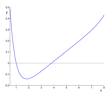
Figure 1: Graph of $f(x)$

So there exist at least two inversive distance circle packing metrics with the same constant $R$-curvature on $\mathbb{S}^{2}$ with the tetrahedral triangulation and inversive distance $I\equiv 2$. $\blacksquare$

Remark 5.

In [25], Ma and Schlenker proved that there is no rigidity for the spherical inversive distance circle packing metrics, which is also valid for the case we discuss in the paper, so we focus on the Euclidean and hyperbolic background geometry only.

4 Combinatorial Ricci flow

Given a closed triangulated surface $(M,\mathcal{T})$ with inversive distance $I\geq 0$, it is natural to consider the following Yamabe problem for the combinatorial curvature $R$.

Yamabe Problem: Does there exist an inversive distance circle packing metric with constant combinatorial $R$-curvature or with prescribed combinatorial $R$-curvature $\overline{R}$? Furthermore, how to find it?

Given $\overline{R}\in C(V)$, if there exists some $\overline{r}\in\Omega$ with $R(\overline{r})=\overline{R}$, we call the function $\overline{R}\in C(V)$ admissible.

Following [17], we introduce an interesting combinatorial curvature flow, the combinatorial Ricci flow, to study the problem.

4.1 Euclidean combinatorial Ricci flow

As before, we take $r_{i}^{2}$ as the analogue of the Riemannian metric for the Euclidean background geometry. Then we have the following definition of combinatorial Ricci flow.

Definition 4.1.

Given a closed triangulated surface $(M,\mathcal{T})$ with inversive distance $I\geq 0$. For the Euclidean background geometry, the combinatorial Ricci flow is defined to be

$$\frac{dg_{i}}{dt}=-R_{i}g_{i}$$ (4.1)

with normalization

$$\frac{dg_{i}}{dt}=(R_{av}-R_{i})g_{i},$$ (4.2)

where $g_{i}=r_{i}^{2}$ and $R_{av}=\frac{2\pi\chi(M)}{||r||_{2}^{2}}$.

It is easy to check that, along the Euclidean combinatorial Ricci flow (4.2), the total measure $||r||_{2}^{2}$ of the triangulated surface is invariant. Furthermore, we have the following interesting property for the combinatorial curvature $R_{i}$ along the normalized Euclidean combinatorial Ricci flow (4.2).

Lemma 4.2.

Along the normalized Euclidean combinatorial Ricci flow (4.2), the combinatorial curvature $R$ evolves according to

$$\frac{dR_{i}}{dt}=\Delta R_{i}+R_{i}(R_{i}-R_{av}),$$ (4.3)

where the Laplace operator $\Delta$ is defined to be

$$\Delta f_{i}=\frac{1}{r_{i}^{2}}\sum_{j=1}^{N}\left(-\frac{\partial K_{i}}{\partial u_{j}}\right)f_{j}=\frac{1}{r_{i}^{2}}\sum_{j\sim i}\left(-\frac{\partial K_{i}}{\partial u_{j}}\right)(f_{j}-f_{i})$$ (4.4)

for $f\in C(V)$, where $u_{i}=\ln r_{i}^{2}$.

Proof. Note that $\frac{\partial}{\partial u_{j}}=\frac{\partial r_{j}}{\partial u_{j}}\frac{\partial}{\partial r_{j}}=\frac{1}{2}r_{j}\frac{\partial}{\partial r_{j}}$, we have

$$\frac{\partial R_{i}}{\partial u_{j}}=\frac{\partial}{\partial u_{j}}(\frac{K_{i}}{r_{i}^{2}})=\frac{1}{r_{i}^{2}}\frac{\partial K_{i}}{\partial u_{j}}-\frac{K_{i}}{r_{i}^{4}}\frac{1}{2}r_{j}\cdot 2r_{i}\delta_{ij}=\frac{1}{r_{i}^{2}}\frac{\partial K_{i}}{\partial u_{j}}-R_{i}\cdot\frac{r_{j}}{r_{i}}\delta_{ij}.$$

Then along the normalized combinatorial Ricci flow (4.2), we have

$$\frac{dR_{i}}{dt}= \sum_{j}\frac{\partial R_{i}}{\partial u_{j}}\frac{du_{j}}{dt}$$

$$= \sum_{j}(\frac{1}{r_{i}^{2}}\frac{\partial K_{i}}{\partial u_{j}}-R_{i}\cdot\frac{r_{j}}{r_{i}}\delta_{ij})(R_{av}-R_{j})$$

$$= \frac{1}{r_{i}^{2}}\sum_{j}(-\frac{\partial K_{i}}{\partial u_{j}})R_{j}+R_{i}(R_{i}-R_{av})$$

$$= \Delta R_{i}+R_{i}(R_{i}-R_{av}),$$

where Lemma 2.1 is used in the third line. $\blacksquare$

Remark 6.

It is very interesting that the evolution equation (4.3) for the combinatorial curvature $R$ along the normalized combinatorial Ricci flow (4.2) is a reaction-diffusion equation and has almost the same form of the evolution of the scalar curvature along the smooth surface Ricci flow obtained by Hamilton [21]. However, as noted by Guo [20], the coefficient in the Laplacian operator in (4.4) may be negative, which leads to that the discrete maximal principle in [17] is not valid here.

Remark 7.

The Laplace operator $\Delta$ could be written in the following matrix form

$$\Delta=-\Sigma^{-1}L$$

where $\Sigma=diag\{r_{1}^{2},\cdots,r_{N}^{2}\}$. As $\Sigma$ is a diagonal matrix, we have

$$-\Delta=\Sigma^{-1}L\sim\Sigma^{\frac{1}{2}}\cdot\Sigma^{-1}L\cdot\Sigma^{-\frac{1}{2}}=\Sigma^{-\frac{1}{2}}L\Sigma^{-\frac{1}{2}},$$

which is conjugate to $L$ and positive semi-definite. By the property of $L$ in Lemma 2.1, we have $-\Delta$ has one eigenvalue $0$ and all other eigenvalues positive, which is similar to the case of eigenvalues of Laplacian operators on Riemannian manifolds. So we can also define the first eigenvalue $\lambda_{1}(\Delta)$ of the discrete Laplace operator $\Delta$ as the smallest positive number $\lambda$ satisfying $-\Delta f=\lambda f$ for some $f\in C(V)$ with $f\not\equiv 0$. We can also define the $n$th eigenvalue $\lambda_{n}(\Delta)$ similarly.

Now we study the long time behavior of the combinatorial Ricci flow. Firstly, we have the following result.

Proposition 4.3.

Given a closed triangulated surface $(M,\mathcal{T})$ with inversive distance $I\geq 0$. If the solution of the Euclidean combinatorial Ricci flow (4.2) stays in $\Omega$ and converges to an inversive distance circle packing metric $r^{*}\in\Omega$, then there exists a constant $R$-curvature metric in $\Omega$ and $r^{*}$ is such one.

Proof. Suppose $u^{*}$ is the corresponding $u$-coordinate of $r^{*}$, i.e. $u^{*}_{i}=\ln r^{*2}_{i}$. Then $R(t)\rightarrow R(u^{*})$ by the continuity of the curvature. As $u(t)\rightarrow u^{*}\in\mathcal{U}$, there exists $\xi_{n}\in(n,n+1)$ such that

$$u(n+1)-u(n)=u^{\prime}(\xi_{n})=(R_{av}-R_{i})|_{\xi_{n}}\rightarrow 0$$

as $n\rightarrow+\infty$, which implies $R(u^{*})=R_{av}$ and $r^{*}$ is a constant curvature metric in $\Omega$. $\blacksquare$

Proposition 4.3 shows that the existence of a constant $R$-curvature metric is necessary for the convergence of the Euclidean combinatorial Ricci flow (4.2). Conversely, we want to know the behavior of the combinatorial Ricci flow under the existence of a constant curvature metric. However, the combinatorial Ricci flow may develop singularities, which can be separated into two types as follows.

Definition 4.4.

Given a closed triangulated surface $(M,\mathcal{T})$ with inversive distance $I\geq 0$. Suppose the solution of the normalized Euclidean combinatorial Ricci flow (4.2) exists on $[0,\tau)$, where $\tau\leq+\infty$.

(1)

The normalized Euclidean combinatorial Ricci flow (4.2) is said to develop an essential singularity at time $\tau$ if there is a vertex $i\in V$ such that $r_{i}(t_{n})$ tends to zero for some time sequence $t_{n}\rightarrow\tau$.

(2)

The normalized Euclidean combinatorial Ricci flow (4.2) is said to develop a removable singularity at $\tau$ if there is a sequence of time $t_{n}\rightarrow\tau$ such that $r(t_{n})$ stay in a compact set of $\mathds{R}^{N}_{>0}$ and there is a triangle $\triangle ijk\in F$ such that the triangle inequalities degenerate as $t_{n}\rightarrow\tau$.

It is interesting that the essential singularity will not develop along the normalized Euclidean combinatorial Ricci flow (4.2), under the existence of a nonpositive constant curvature metric. Before presenting the result, we state the following property for the extended Ricci potential function $\widetilde{F}$.

Proposition 4.5.

Given a closed triangulated surface $(M,\mathcal{T})$ with inversive distance $I\geq 0$ and $\chi(M)\leq 0$. Suppose there exists a Euclidean inversive distance circle packing metric $r^{*}\in\Omega$ with constant $R$-curvature and define the extended Ricci potential function $\widetilde{F}(u)$ on $\mathds{R}^{N}$ as

$$\widetilde{F}(u)=-\sum_{\Delta ijk\in F}\widetilde{F}_{ijk}(u)+\int_{u^{*}}^{u}\sum_{i=1}^{N}(2\pi-R_{av}r_{i}^{2})du_{i},$$ (4.5)

where

$$\widetilde{F}_{ijk}(u)=\int_{u^{*}}^{u}\widetilde{\theta}_{i}du_{i}+\widetilde{\theta}_{j}du_{j}+\widetilde{\theta}_{k}du_{k}.$$

Then $\widetilde{F}(u+t\textbf{1})=\widetilde{F}(u)$ and $\nabla_{u_{i}}\widetilde{F}=\widetilde{K}_{i}-R_{av}r_{i}^{2}$, where $\widetilde{K}_{i}=2\pi-\sum_{\triangle ijk\in F}\widetilde{\theta}_{i}$. Set $\mathcal{U}_{a}=\{u\in\mathds{R}^{N}|\sum_{i}u_{i}=a\},a\in\mathds{R}$. Then $\widetilde{F}|_{\mathcal{U}_{a}}$ is convex and proper. $\widetilde{F}|_{\mathcal{U}_{a}}$ has a unique zero point which is the unique minimal point of $\widetilde{F}|_{\mathcal{U}_{a}}$. Furthermore, $\lim_{u\in\mathcal{U}_{a},u\rightarrow\infty}\widetilde{F}(u)=+\infty$.

Proof. By the definition of $\tilde{\theta}$, we have $\tilde{\theta}_{i}+\tilde{\theta}_{j}+\tilde{\theta}_{k}=\pi$ for any topological triangle $\triangle ijk\in F$. As the value of $\widetilde{F}_{ijk}(u)$ is independent of the path from $u^{*}$ to $u$, it is easy to check $\widetilde{F}_{ijk}(u+t\textbf{1})=\widetilde{F}_{ijk}(u)+t\pi$ by the scaling invariance of $\widetilde{\theta}$ with respect to $r$. Then we have

$$\widetilde{F}(u+t\textbf{1})-\widetilde{F}(u)= -\pi|F|t+\int_{u}^{u+t\textbf{1}}\sum_{i=1}^{N}(2\pi-R_{av}r_{i}^{2})du_{i}$$

$$= -\pi|F|t+(2\pi|V|-2\pi\chi(M))t$$

$$= 0.$$

It is also easy to check that

$$\nabla_{u_{i}}\widetilde{F}=-\sum_{\triangle ijk\in F}\widetilde{\theta}_{i}^{jk}+2\pi-R_{av}r_{i}^{2}=\widetilde{K}_{i}-R_{av}r_{i}^{2}$$

and

$$\operatorname{Hess}_{u}\widetilde{F}|_{\mathcal{U}}=L-R_{av}\Sigma^{\frac{1}{2}}\left(I-\frac{rr^{T}}{||r||^{2}}\right)\Sigma^{\frac{1}{2}}=\Sigma^{\frac{1}{2}}\left(\Lambda-R_{av}\left(I-\frac{rr^{T}}{||r||^{2}}\right)\right)\Sigma^{\frac{1}{2}},$$

where $\Sigma=diag\{r_{1}^{2},\cdots,r_{N}^{2}\}$, $\Lambda=\Sigma^{-\frac{1}{2}}L\Sigma^{-\frac{1}{2}}$. Note that $\Lambda$ is positive semi-definite with $rank=N-1$ and kernel $\{cr|c\in\mathds{R}\}$ by Lemma 2.1, we have $\operatorname{Hess}_{u}\widetilde{F}|_{\mathcal{U}}$ is positive semi-definite with $rank=N-1$ and kernel $\{c\textbf{1}|c\in\mathds{R}\}$ under the condition $\chi(M)\leq 0$. This implies that $\operatorname{Hess}_{u}\widetilde{F}|_{\mathcal{U}\cap\mathcal{U}_{a}}$ is strictly positive definite and $\widetilde{F}|_{\mathcal{U}\cap\mathcal{U}_{a}}$ is strictly convex. By the concavity of $\widetilde{F}_{ijk}$ and the condition $\chi(M)\leq 0$, it is easy to check that $\widetilde{F}$ is $C^{1}$ smooth and convex. Combining with $\widetilde{F}(u+t\textbf{1})=\widetilde{F}(u)$, we have $\widetilde{F}|_{\mathcal{U}_{a}}$ is a $C^{1}$ smooth convex function and strictly convex on $\mathcal{U}\cap\mathcal{U}_{a}$ under the condition $\chi(M)\leq 0$.

The existence of a constant curvature metric $r^{*}$ ensures that the corresponding $u^{*}\in\mathcal{U}\cap\mathcal{U}_{a}$ is a critical point of $\widetilde{F}|_{\mathcal{U}_{a}}$. Then the rest of the proof follows from applying the following Lemma 4.6 to the convex function $\widetilde{F}|_{\mathcal{U}_{a}}$. $\blacksquare$

Lemma 4.6.

Suppose $f(x)$ is a $C^{1}$ smooth convex function on $\mathds{R}^{n}$ with $\nabla f(x_{0})=0$ for some $x_{0}\in\mathds{R}^{n}$, $f(x)$ is $C^{2}$ smooth and strictly convex in a neighborhood of $x_{0}$, then $\lim_{x\rightarrow\infty}f(x)=+\infty$.

Proof. Without loss of generality, we can assume $x_{0}=0$, otherwise parallel translating $x_{0}$ to $0$. Suppose $f(x)$ is $C^{2}$ smooth and strictly convex on the ball $B(0,\epsilon)$ for some constant $\epsilon>0$. For any $v\in\mathbb{S}^{n-1}$, we have $f_{v}(t)=f(tv)$ is a $C^{1}$ smooth convex function in $t$ and $f_{v}^{\prime}(0)=0$. Furthermore, $f_{v}(t)$ is strictly convex on $[0,\epsilon]$ since $f(x)$ is strictly convex on $B(0,\epsilon)$. Then, for $t>\epsilon$, we have

$$f_{v}(t)\geq f_{v}(\epsilon)+f_{v}^{\prime}(\epsilon)(t-\epsilon).$$

Therefore, for any $x\in\mathds{R}^{n}$ with $||x||>\epsilon$, we have

$$f(x)=f(||x||\frac{x}{||x||})=f_{\frac{x}{||x||}}(||x||)\geq f_{\frac{x}{||x||}}(\epsilon)+f_{\frac{x}{||x||}}^{\prime}(\epsilon)(||x||-\epsilon).$$ (4.6)

Note that

$$f_{\frac{x}{||x||}}(\epsilon)=f(\epsilon\frac{x}{||x||})\geq min_{v\in\mathbb{S}^{n-1}}f(\epsilon v)=c_{1}>0.$$ (4.7)

Furthermore, for any $v\in\mathbb{S}^{n-1}$, $f_{v}^{\prime}(\epsilon)>0$ by the strict convexity of $f_{v}(t)$ on $[0,\epsilon]$ and $f_{v}^{\prime}(0)=0$, so we have

$$f_{\frac{x}{||x||}}^{\prime}(\epsilon)\geq min_{v\in\mathbb{S}^{n-1}}f_{v}^{\prime}(\epsilon)=c_{2}>0.$$ (4.8)

Combining (4.6), (4.7) and (4.8), we have

$$f(x)\geq c_{1}+c_{2}(||x||-\epsilon)$$

for some $c_{1},c_{2}>0$ and any $x\in\mathds{R}^{n}$ with $||x||>\epsilon$, which implies $\lim_{x\rightarrow\infty}f(x)=+\infty$. $\blacksquare$

Remark 8.

In fact, the proof of Proposition 4.5 shows that, under the conditions of Proposition 4.5, the constant curvature metric $r^{*}\in\Omega$ is the unique inversive distance circle packing metric with constant $\widetilde{R}$-curvature in $\mathds{R}^{N}_{>0}$ (up to scaling in the case of $\chi(M)=0$).

Note that $||r||_{2}^{2}=\sum_{i=1}^{2}$ is invariant along the (4.2), we assume that $r(0)\in\mathbb{S}^{N-1}\cap\Omega$ in the following. Set

$$\mathcal{S}=\{u\in\mathds{R}^{N}|\sum_{i=1}^{N}e^{u_{i}}=1\}.$$

Using the property $\widetilde{F}(u+t\textbf{1})=\widetilde{F}(u)$, we have the following property for the extended Ricci potential $\widetilde{F}(u)$.

Corollary 4.7.

Given a closed triangulated surface $(M,\mathcal{T})$ with inversive distance $I\geq 0$ and $\chi(M)\leq 0$. Suppose there exists a Euclidean inversive distance circle packing metric $r^{*}\in\Omega$ with constant $R$-curvature. Then $\widetilde{F}|_{\mathcal{S}}$ is proper. Furthermore, $\lim_{u\rightarrow\infty}\widetilde{F}|_{\mathcal{S}}=+\infty$.

Proof. Let $\Pi$ be the orthogonal projection from $\mathcal{S}$ to the plane $\mathcal{U}_{0}$. Then for a sequence $u^{(n)}\in\mathcal{S}$, $\Pi(u^{(n)})$ is unbounded if and only if $|\Pi(u^{(n)})_{i}-\Pi(u^{(n)})_{j}|=|u^{(n)}_{i}-u^{(n)}_{j}|$ is unbounded. If $u\in\mathcal{S}$ and $u\rightarrow\infty$, we have $\Pi(u)\rightarrow\infty$. Then $\widetilde{F}(u)=\widetilde{F}(\Pi(u))\rightarrow\infty$. $\blacksquare$

Now we can get the following result on nonexistence of essential singularities along the normalized Euclidean combinatorial Ricci flow.

Theorem 4.8.

Given a closed triangulated surface $(M,\mathcal{T})$ with inversive distance $I\geq 0$ and $\chi(M)\leq 0$. If there exists a Euclidean inversive distance circle packing metric $r^{*}\in\Omega$ with constant $R$-curvature, then the solution of the combinatorial Ricci flow (4.2) develop no essential singularities.

Proof. To prove the result, we need to extend the combinatorial Ricci flow to the following form

$$\frac{dg_{i}}{dt}=(R_{av}-\widetilde{R}_{i})g_{i},$$ (4.9)

where $\widetilde{R}_{i}=\frac{\widetilde{K}_{i}}{r_{i}^{2}}$ with $\widetilde{K}_{i}=2\pi-\sum_{\Delta ijk\in F}\widetilde{\theta}_{i}^{jk}$. The equation (4.9) could be written as

$$\frac{du_{i}}{dt}=R_{av}-\widetilde{R}_{i}.$$ (4.10)

Note that $R_{av}-\widetilde{R}_{i}$ is just a continuous function of $u\in\mathds{R}^{N}$ and not locally Lipschiz in $u\in\mathds{R}^{N}$. By the existence of solution of ODE for continuous function, there exists at least one solution of (4.9). There may be no uniqueness for the solution of the extended flow (4.9) on $\mathds{R}^{N}$. However, note that $\widetilde{R}|_{\mathcal{U}}=R$ on $\mathcal{U}$ and $R$ is locally Lipschitz, so the solutions of (4.2) and (4.10) agree on $\mathcal{U}$ by Picard’s uniqueness for the solution of ODE. And then any solution of (4.10) extends the solution of (4.2).

Under the assumption of the existence of the constant curvature metric, the Ricci potential

$$\widetilde{F}(u)=-\sum_{\Delta ijk\in F}\widetilde{F}_{ijk}(u)+\int_{u^{*}}^{u}\sum_{i=1}^{N}(2\pi-R_{av}r_{i}^{2})du_{i},$$

is convex. Note that $\widetilde{F}|_{\mathcal{S}}$ is proper, $\lim_{u\rightarrow\infty}\widetilde{F}|_{\mathcal{S}}(u)=+\infty$ and

$$\frac{d}{dt}\widetilde{F}(u(t))=-\sum_{i=1}^{N}(\widetilde{R}_{i}-R_{av})^{2}r_{i}^{2}\leq 0$$

along the extended Ricci flow (4.10), we have the solution $u(t)$ of the extended flow (4.10) stays in a compact subset of $\mathds{R}^{N}$, which implies that the solution $r_{i}(t)$ of (4.9) has uniform positive lower and upper bounds for any $i\in V$ and $t\in\mathds{R}$. As the solution of (4.9) extends the solution of the combinatorial Ricci flow (4.2), we have the solution of the combinatorial Ricci flow (4.2) will not develop essential singularities. $\blacksquare$

Theorem 4.8 shows that there is no essential singularities along the normalized Euclidean combinatorial Ricci flow (4.2) in finite time and at time infinity. If the flow (4.2) further develops no removable singularities, we have the following interesting result.

Theorem 4.9.

Given a closed triangulated surface $(M,\mathcal{T})$ with inversive distance $I\geq 0$ and $\chi(M)\leq 0$. If there exists a Euclidean inversive distance circle packing metric $r^{*}\in\Omega$ with constant $R$-curvature and the solution of the combinatorial Ricci flow (4.2) develops no removable singularities in finite time, then the solution converges exponentially fast to the constant curvature metric.

Proof. The proof of Theorem (4.8) shows that the solution of (4.2) and (4.9) stays in a compact subset of $\mathds{R}^{N}_{>0}$. This implies the solution of (4.2) and (4.9) exists for all time. $u(t)$ is bounded implies that the function $\widetilde{F}(u(t))$ is bounded along the flow. Note that

$$\frac{d}{dt}\widetilde{F}(u(t))=\sum_{i=1}^{N}\nabla_{u_{i}}\widetilde{F}\cdot\frac{du_{i}}{dt}=\sum_{i=1}^{N}(K_{i}-R_{av}r_{i}^{2})(R_{av}-R_{i})=-\sum_{i=1}^{N}(R_{av}-R_{i})^{2}r_{i}^{2}\leq 0,$$

we have $\lim_{t\rightarrow+\infty}\widetilde{F}(u(t))$ exists. Then

$$\widetilde{F}(u(n+1))-\widetilde{F}(u(n))=-\sum_{i=1}^{N}(R_{av}-\widetilde{R}_{i})^{2}r_{i}^{2}|_{t=\xi_{n}}\rightarrow 0$$ (4.11)

as $n\rightarrow+\infty$, for some $\xi_{n}\in(n,n+1)$. As $r(\xi_{n})$ is bounded, then there exists a subsequence, still denoted as $r(\xi_{n})$, such that $r(\xi_{n})\rightarrow\bar{u}$ and then $\widetilde{R}(r(\xi_{n}))\rightarrow\widetilde{R}(\bar{r})$. The equation (4.11) shows that $\widetilde{R}(\bar{r})=R_{av}$. By the uniqueness of constant curvature metric in $\mathds{R}^{N}_{>0}$ in Remark 8, we have $\bar{r}=r^{*}\in\Omega$.

Furthermore, $r^{*}$ is a local attractor of the equation (4.2). In fact, the equation (4.2) could be written as

$$\frac{dr_{i}}{dt}=\frac{1}{2}(R_{av}-R_{i})r_{i}.$$

Set $\Gamma_{i}(r)=\frac{1}{2}(R_{av}-R_{i})r_{i}$, then we have

$$D_{r}\Gamma|_{r^{*}}=R_{av}\left(I-\frac{rr^{T}}{||r||^{2}}\right)-\Sigma^{-\frac{1}{2}}L\Sigma^{-\frac{1}{2}}=R_{av}\left(I-\frac{rr^{T}}{||r||^{2}}\right)-\Lambda,$$

where $\Sigma=diag\{r_{1}^{2},\cdots,r_{N}^{2}\}$ and $\Lambda=\Sigma^{-\frac{1}{2}}L\Sigma^{-\frac{1}{2}}\sim\Sigma^{-\frac{1}{2}}\Lambda\Sigma^{\frac{1}{2}}=-\Delta$. Select an orthonormal matrix $P$ such that

$$P^{T}\Lambda P=diag\{0,\lambda_{1}(\Lambda),\cdots,\lambda_{N-1}(\Lambda)\}.$$

Suppose $P=(e_{0},e_{1},\cdots,e_{N-1})$, where $e_{i}$ is the $(i+1)$-column of $P$. Then $\Lambda e_{0}=0$ and $\Lambda e_{i}=\lambda_{i}e_{i},\,1\leq i\leq N-1$, which implies $e_{0}=r/\|r\|$ and $r\perp e_{i},\,1\leq i\leq N-1$. Hence $\big{(}I_{N}-\frac{rr^{T}}{\|r\|^{2}}\big{)}e_{0}=0$ and $\big{(}I_{N}-\frac{rr^{T}}{\|r\|^{2}}\big{)}e_{i}=e_{i}$, $1\leq i\leq N-1$, which implies $P^{T}\big{(}I_{N}-\frac{rr^{T}}{\|r\|^{2}}\big{)}P=diag\{0,1,\cdots,1\}$. Therefore,

$$D_{r}\Gamma\big{|}_{r^{*}}=P\cdot diag\{0,R_{av}-\lambda_{1}(\Lambda),\cdots,R_{av}-\lambda_{N-1}(\Lambda)\}\cdot P^{T}.$$

Note that $\lambda_{1}(\Lambda)>R_{av}^{*}=\frac{2\pi\chi(M)}{||r^{*}||^{2}}$ in the case of $\chi(M)\leq 0$, then $D_{r}\Gamma\big{|}_{r^{*}}$ is negative semi-definite with kernel $\{cr|c\in\mathbb{R}\}$ and $rank\,(D_{r}\Gamma\big{|}_{r^{*}})=N-1$. Note that, along the flow (4.2), $||r||^{2}$ is invariant. Thus the kernel is transversal to the flow. This implies that $D_{r}\Gamma|_{r^{*}}$ is negative definite on $\mathbb{S}^{N-1}$ and $r^{*}$ is a local attractor of the normalized combinatorial Ricci flow (4.2). Then the conclusion follows from the Lyapunov Stability Theorem([26], Chapter 5) and the fact that $r(\xi_{n})\rightarrow r^{*}$. $\blacksquare$

Remark 9.

The proof of Theorem 4.9 shows that the solution of (4.2) will not develop any removable singularity at time infinity.

Remark 10.

Note that $\Lambda=\Sigma^{-\frac{1}{2}}L\Sigma^{-\frac{1}{2}}\sim\Sigma^{-\frac{1}{2}}\Lambda\Sigma^{\frac{1}{2}}=-\Delta$, to ensure the local convergence of the flow (4.2), we only need the first eigenvalue of the discrete Laplace operator satisfying $\lambda_{1}(\Delta)|_{r^{*}}>R_{av}$, which is obvious in the case of $\chi(M)\leq 0$.

The only case left is that the solution of the normalized combinatorial Ricci flow (4.2) develops removable singularities at finite time, which implies that there exists some triangle $\triangle ijk\in F$ degenerating as $t\rightarrow\tau$. The proof of Theorem 4.9 suggests us to use the extended combinatorial Ricci flow (4.9) to characterize the existence of the constant curvature metric. In fact, we have the following main theorem.

Theorem 4.10.

Given a closed triangulated surface $(M,\mathcal{T})$ with inversive distance $I\geq 0$ and $\chi(M)\leq 0$. If there exists an inversive distance circle packing metric $r^{*}\in\Omega$ with constant $R$-curvature, then the solution of the extended combinatorial Ricci flow (4.9) exists for all time and converges exponentially fast to the constant curvature metric $r^{*}$.

The proof of Theorem 4.10 is almost the same as that of Theorem 4.9, we omit the details here. And in the special case that the solution of the normalized combinatorial Ricci flow (4.2) stays in $\Omega$, this is just Theorem 4.9.

Remark 11.

As there maybe exist more than one solution for the extended flow (4.9) and every solution of (4.9) extends the solution of the combinatorial Ricci flow (4.2), Theorem 4.10 shows that every such solution will go back into $\Omega$ and converges to the constant curvature metric. Furthermore, as $\partial\Omega$ is piecewise analytic and the solution of the extended flow (4.9) is $C^{1}$ smooth, any solution of (4.9) intersects $\partial\Omega$ at most finite times.

Remark 12.

The existence of removable singularity along the normalized combinatorial Ricci flow suggests a way to do surgery on the triangulated surface, as stated by Luo in [23]. And this way should be also valid here. However, surgeries on the triangulated surface change the combinatorial structure on the triangulated surface. If there exists a constant curvature metric on the triangulated surface with given combinatorial structure and the solution of the extended flow (4.9) develops a removable singularity at finite time, surgeries on the triangulated surface shall give a constant curvature metric with a different combinatorial structure. However, Theorem 4.10 ensures that we can find the constant curvature metric $r^{*}\in\Omega$ with the given combinatorial structure under the existence of a constant curvature metric, even if the solution of the normalized combinatorial Ricci flow (4.2) develops removable singularities at finite time.

We can also use the Euclidean combinatorial flow to study the prescribing curvature problem of the $R$-curvature. As the proof is almost parallel to the case of constant curvature metric problem, we just summarize the results in the following theorem and omit its proof.

Theorem 4.11.

Given a closed triangulated surface $(M,\mathcal{T})$ with inversive distance $I\geq 0$ and $\chi(M)\leq 0$. $\overline{R}\in C(V)$ is a given function on $(M,\mathcal{T})$.

(1)

If the solution of the modified Euclidean combinatorial Ricci flow

$$\frac{dg_{i}}{dt}=(\overline{R}_{i}-R_{i})g_{i},$$ (4.12)

where $g_{i}=r_{i}^{2}$, stays in $\Omega$ and converges to an inversive distance circle packing metric $\overline{r}\in\Omega$, then $R(\overline{r})=\overline{R}$ and $\overline{R}$ is admissible.

(2)

Suppose $\overline{R}\in C(V)$ is admissible with $R(\overline{r})=\overline{R}$ for some $\overline{r}\in\Omega$, $\overline{R}\leq 0$ and $\overline{R}\not\equiv 0$, then the modified Euclidean combinatorial Ricci flow (4.12) does not develop essential singularities in finite time and at time infinity. Furthermore, if the solution of (4.12) develops no removable singularities in finite time, then the solution of (4.12) exists for all time, converges exponentially fast to $\overline{r}$ and does not develop removable singularities at time infinity.

(3)

Suppose $\overline{R}\in C(V)$ is admissible with $R(\overline{r})=\overline{R}$ for some $\overline{r}\in\Omega$, $\overline{R}\leq 0$ and $\overline{R}\not\equiv 0$, then the solution of the extended modified Euclidean combinatorial Ricci flow

$$\frac{dg_{i}}{dt}=(\overline{R}_{i}-\widetilde{R}_{i})g_{i}$$

exists for all time and converges exponentially fast to $\overline{r}$.

Remark 13.

The case of $\overline{R}\equiv 0$ is just the constant curvature problem, so we do not include it in Theorem 4.11 here. Theorem 4.11 provided an effective way to find an inversive distance circle packing metric with given prescribed curvature and given combinatorial structure.

4.2 Hyperbolic combinatorial Ricci flow

For the hyperbolic background geometry, we take $\tanh^{2}\frac{r_{i}}{2}$ as the analogue of the Riemannian metric. Then we have the following definition of hyperbolic combinatorial Ricci flow.

Definition 4.12.

Given a closed triangulated surface $(M,\mathcal{T})$ with inversive distance $I\geq 0$. For the hyperbolic background geometry, the combinatorial Ricci flow is defined as

$$\frac{dg_{i}}{dt}=-R_{i}g_{i},$$ (4.13)

where $g_{i}=\tanh^{2}\frac{r_{i}}{2}$. Given a function $\overline{R}\in C(V)$, the modified combinatorial Ricci flow is defined to be

$$\frac{dg_{i}}{dt}=(\overline{R}_{i}-R_{i})g_{i}.$$ (4.14)

Similar to the Euclidean background geometry, we have the following evolution of the hyperbolic combinatorial curvature $R$ along the modified hyperbolic combinatorial Ricci flow.

Lemma 4.13.

Along the modified hyperbolic combinatorial Ricci flow (4.14), the combinatorial curvature $R_{i}$ evolves according to

$$\frac{dR_{i}}{dt}=-\frac{1}{\tanh^{2}\frac{r_{i}}{2}}\sum_{j}\frac{\partial K_{i}}{\partial u_{j}}(R_{j}-\overline{R}_{j})+R_{i}(R_{i}-\overline{R}_{i}),$$

where $u_{i}=\ln\tanh^{2}\frac{r_{i}}{2}$.

Proof. As $u_{i}=\ln\tanh^{2}\frac{r_{i}}{2}$, we have

$$du_{i}=\frac{2}{\tanh\frac{r_{i}}{2}}\cdot\frac{1}{\cosh^{2}\frac{r_{i}}{2}}\cdot\frac{1}{2}dr_{i}=\frac{2}{\sinh r_{i}}dr_{i},$$

which implies that $\frac{\partial}{\partial u_{j}}=\frac{\partial r_{j}}{\partial u_{j}}\frac{\partial}{\partial r_{j}}=\frac{1}{2}\sinh r_{j}\frac{\partial}{\partial r_{j}}$. So we have

$$\frac{dR_{i}}{dt}= \sum_{j}\frac{\partial R_{i}}{\partial u_{j}}\frac{du_{j}}{dt}$$

$$= \sum_{j}\left(\frac{1}{\tanh^{2}\frac{r_{i}}{2}}\frac{\partial K_{i}}{\partial u_{j}}-\frac{1}{2}\sinh r_{j}\cdot\frac{R_{i}}{\tanh^{2}\frac{r_{i}}{2}}\cdot 2\tanh\frac{r_{i}}{2}\frac{1}{\cosh^{2}\frac{r_{i}}{2}}\cdot\frac{1}{2}\delta_{ij}\right)(\overline{R}_{j}-R_{j})$$

$$= \sum_{j}\left(\frac{1}{\tanh^{2}\frac{r_{i}}{2}}\frac{\partial K_{i}}{\partial u_{j}}-\frac{\sinh r_{j}}{\sinh r_{i}}R_{i}\delta_{ij}\right)(\overline{R}_{j}-R_{j})$$

$$= -\frac{1}{\tanh^{2}\frac{r_{i}}{2}}\sum_{j}\frac{\partial K_{i}}{\partial u_{j}}(R_{j}-\overline{R}_{j})+R_{i}(R_{i}-\overline{R}_{i}).$$

$\blacksquare$

Different from the case of Euclidean background geometry, we just consider the prescribing curvature problem in the case of hyperbolic background geometry using the modified hyperbolic combinatorial Ricci flow (4.14) following [18], which includes the constant curvature problem with the constant being zero. First, we have the following necessary condition for the convergence of the flow.

Proposition 4.14.

Given a closed triangulated surface $(M,\mathcal{T})$ with inversive distance $I\geq 0$. If the solution of the modified hyperbolic combinatorial Ricci flow (4.14) stays in $\Omega$ and converges to $\overline{r}\in\Omega$, then we have $\overline{R}$ is admissible and $R(\overline{r})=\overline{R}$.

The proof of Proposition 4.14 is similar to that of Proposition 4.3, we omit it here.

Conversely, assuming the admissibility of $\overline{R}$, we have results similar to that of the Euclidean background case. Before presenting the results, we state the following useful lemma which we need in the following, which is given in [7, 18] and still valid in the case of inversive distance circle packing metric with $I\geq 0$.

Lemma 4.15.

Given a hyperbolic triangle $\triangle v_{i}v_{j}v_{k}$, which is constructed by inversive distance circle packing metric $r$ with inversive distance $I\geq 0$. For any $\epsilon>0$, there exists a number $l>0$ such that when $r_{i}>l$, the inner angle $\theta_{i}$ at the vertex $v_{i}$ of the hyperbolic triangle $\triangle v_{i}v_{j}v_{k}$ is smaller than $\epsilon$.

The proof of Lemma 4.15 is the same as that of Lemma 3.2 in [18], we omit it here. Note that the convergence result in Lemma 4.15 is in fact the uniform convergence of $\theta_{i}^{jk}$ with respect to $r_{i}$, assuming that the triangle inequalities are satisfied.

We further have the following interesting result on triangle inequalities.

Lemma 4.16.

Given a topological triangle $\triangle ijk\in F$ with the lengths given by (2.2) and inversive distance $I\geq 0$, there exists a positive number $l=l(I_{jk})$ such that if $r_{i}>l$, then $l_{ij}+l_{ik}>l_{jk}$.

Proof. We just need to prove $\cosh(l_{ij}+l_{ik})>\cosh l_{jk}$. Note that there exists $l>0$ such that if $r_{i}>l$, then $\cosh^{2}r_{i}>I_{jk}+1$. Then we have

$$\cosh(l_{ij}+l_{ik})> \cosh l_{ij}\cosh l_{ik}$$

$$= (\cosh r_{i}\cosh r_{j}+I_{ij}\sinh r_{i}\sinh r_{j})(\cosh r_{i}\cosh r_{k}+I_{ik}\sinh r_{i}\sinh r_{k})$$

$$> \cosh^{2}r_{i}\cosh r_{j}\cosh r_{k}$$

$$> (I_{jk}+1)\cosh r_{j}\cosh r_{k}$$

$$\geq \cosh r_{j}\cosh r_{k}+I_{jk}\sinh r_{j}\sinh r_{k}$$

$$= \cosh l_{jk}.$$

$\blacksquare$

Combining Lemma 4.15 and Lemma 4.16, we have

Lemma 4.17.

Given a topological triangle $\triangle ijk\in F$ with the lengths given by (2.2) with inversive distance $I\geq 0$. For any $\epsilon>0$, there exists a positive number $l=l(I_{jk},\epsilon)$ such that if $r_{i}>l$, then the extended inner angle $\widetilde{\theta}_{i}^{jk}<\epsilon$.

Proof. By Lemma 4.16, there exists $l_{1}>0$ such that $l_{ij}+l_{ik}>l_{jk}$. If the other two triangle inequalities are not satisfied, then $\widetilde{\theta}_{i}^{jk}=0$. If the other two triangle inequalities are satisfied, by Lemma 4.15, there exists $l_{2}>0$ such that if $r_{i}>l_{2}$, then $\widetilde{\theta}_{i}^{jk}<\epsilon$. Take $l=\max\{l_{1},l_{2}\}$, then we get the proof of the lemma. $\blacksquare$

Then we have the following main result.

Theorem 4.18.

Given a closed triangulated surface $(M,\mathcal{T})$ with inversive distance $I\geq 0$ and $\chi(M)\leq 0$. $\overline{R}\in C(V)$ is admissible with $R(\overline{r})=\overline{R}$ and $\overline{R}\leq 0$.

(1)

The modified hyperbolic combinatorial Ricci flow (4.14) does not develop essential singularity in finite time and at time infinity.

(2)

If the solution of (4.14) develops no removable singularities in finite time, then the solution of (4.14) exists for all time, converges exponentially fast to $\overline{r}$ and does not develop removable singularities at time infinity.

(3)

Any solution of the extended hyperbolic flow

$$\frac{dg_{i}}{dt}=(\overline{R}_{i}-\widetilde{R}_{i})g_{i}$$

with $g_{i}=\tanh^{2}\frac{r_{i}}{2}$ exists for all time and converges exponentially fast to $\overline{r}$.

Proof.

(1)

Set $u_{i}=\ln\tanh^{2}\frac{r_{i}}{2}$, which maps $\mathds{R}^{N}_{>0}$ onto $\mathds{R}^{N}_{<0}$. Denote $\overline{u}$ as the $u$-coordinate of $\overline{r}$. Consider the Ricci potential function

$$F(u)=-\sum_{\triangle ijk\in F}F_{ijk}(u)+\int_{\overline{u}}^{u}\sum_{i=1}^{N}(2\pi-\overline{R}_{i}\tanh^{2}\frac{r_{i}}{2}),$$

which is strictly convex on $\mathcal{U}$ in the case of $\overline{R}\leq 0$ and could be extended to a $C^{1}$ smooth convex function

$$\widetilde{F}(u)=-\sum_{\triangle ijk\in F}\widetilde{F}_{ijk}(u)+\int_{\overline{u}}^{u}\sum_{i=1}^{N}(2\pi-\overline{R}_{i}\tanh^{2}\frac{r_{i}}{2})$$

defined on $\mathds{R}^{N}_{<0}$. By direct calculations, we have

$$\nabla_{u_{i}}\widetilde{F}=\widetilde{K}_{i}-\overline{R}_{i}\tanh^{2}\frac{r_{i}}{2}$$

and $\overline{u}$ is a critical point of $\widetilde{F}$. Note that, in the case of $\overline{R}\leq 0$, we have

$$\operatorname{Hess}_{u}\widetilde{F}|_{\mathcal{U}}=L-\left(\begin{array}[]{ccc}\overline{R}_{1}\tanh^{2}\frac{r_{1}}{2}&&\\ &\ddots&\\ &&\overline{R}_{N}\tanh^{2}\frac{r_{N}}{2}\\ \end{array}\right),$$

which is positive definite by Lemma 2.1. Applying Lemma 4.6, we have $\lim_{u\rightarrow\infty}\widetilde{F}(u)=+\infty$. Along the extended modified hyperbolic combinatorial Ricci flow

$$\frac{dg_{i}}{dt}=(\overline{R}_{i}-\widetilde{R}_{i})g_{i},$$ (4.15)

where $g_{i}=\tanh^{2}\frac{r_{i}}{2}$, we have

$$\frac{d}{dt}\widetilde{F}(u(t))=\nabla_{u}\widetilde{F}\cdot\frac{du}{dt}=-\sum_{i=1}^{N}(\overline{R}_{i}-R_{i})^{2}\tanh^{2}\frac{r_{i}}{2}\leq 0,$$

which implies $\widetilde{F}(u(t))$ is decreasing along the extended hyperbolic flow (4.15). By $\lim_{u\rightarrow\infty}\widetilde{F}(u)=+\infty$, we have the solution $u(t)$ of the extended hyperbolic flow (4.15) is bounded in $\mathds{R}^{N}_{<0}$, and then there exists $c>0$ such that $u_{i}(t)>-c$ for any $i\in V$, which implies $r_{i}(t)\geq\delta=\ln\frac{1+e^{-c}}{1-e^{-c}}>0$. As the solution of the hyperbolic flow (4.14) is always part of the solution of the extended hyperbolic flow (4.15), we have the solution of the hyperbolic flow (4.14) never develops essential singularities.

(2)

In the case that the solution of the hyperbolic Ricci flow (4.14) develops no removable singularities at finite time, the solution of the hyperbolic Ricci flow (4.14) exists for all time. We claim that $r_{i}(t)$ is bounded from above. Otherwise there exists at least one vertex $i\in V$ such that $\limsup_{t\rightarrow\infty}r_{i}(t)=+\infty$. For fixed $i\in V$, using Lemma 4.15, we can choose $l>0$ large enough such that, when $r_{i}>l$, the inner angle $\theta_{i}^{jk}$ is smaller than $\frac{\pi}{d_{i}}$, where $d_{i}$ is the degree of the vertex $i$, which implies $K_{i}=2\pi-\sum_{\triangle ijk\in F}\theta_{i}^{jk}>\pi>0$ and $R_{i}=\frac{K_{i}}{\tanh^{2}\frac{r_{i}}{2}}>0$. Choose a time $t_{0}$ such that $r_{i}(t_{0})>l$, this can be done as we have $\limsup_{t\rightarrow+\infty}r_{i}=+\infty$. Set $a=\inf\{t<t_{0}|r_{i}(s)>l,\forall s\in[t,t_{0}]\}$, then $r_{i}(a)=l$. Note that the hyperbolic Ricci flow (4.14) could be written as

$$\frac{dr_{i}}{dt}=\frac{1}{2}(\overline{R}_{i}-R_{i})\sinh r_{i}.$$

So we have $r_{i}^{\prime}(t)<0$ on $[a,t_{0}]$. Combining with $r_{i}(a)=l$, we have $r_{i}(t_{0})<l$, which contradicts $r_{i}(t_{0})>l$.

The arguments show that the solution $r(t)$ of the hyperbolic Ricci flow (4.14) stays in a compact subset of $\mathds{R}^{N}_{>0}$ if the flow (4.14) develops no removable singularities at finite time. Thus $\widetilde{F}(u(t))$ is bounded and decreasing along the extended hyperbolic flow (4.15), which implies $\lim_{t\rightarrow+\infty}\widetilde{F}(u(t))$ exist. Then there exists $\xi_{n}\in(n,n+1)$ such that

$$\widetilde{F}(u(n+1))-\widetilde{F}(u(n+1))=-\sum_{i=1}^{N}(\overline{R}_{i}-\widetilde{R}_{i})^{2}\tanh^{2}\frac{r_{i}}{2}|_{\xi_{n}}\rightarrow 0.$$

Since the solution $\{r(t)\}\subset\subset\mathds{R}^{N}_{>0}$, $r(\xi_{n})$ have a convergent subsequence, still denoted as $r(\xi_{n})$, with $r(\xi_{n})\rightarrow r^{*}$. Then we have $\widetilde{R}(r^{*})=\overline{R}$. By the uniqueness of $\widetilde{R}$ with respect to $r\in\mathds{R}^{N}_{>0}$ for the case of hyperbolic background geometry as in Remark 3, we have $r^{*}=\overline{r}\in\Omega$.

The rest of the proof is an application of the Lyapunov Theorem to the hyperbolic combinatorial Ricci flow (4.14). Write the hyperbolic combinatorial Ricci flow (4.14) in the form

$$\frac{du_{i}}{dt}=\overline{R}_{i}-R_{i}$$ (4.16)

and set $\Gamma_{i}(u)=\overline{R}_{i}-R_{i}$. Then we have

$$D_{u}\Gamma|_{\overline{u}}=-\Sigma^{-1}L+\left(\begin{array}[]{ccc}\overline{R}_{1}&&\\ &\ddots&\\ &&\overline{R}_{N}\\ \end{array}\right),$$

whose eigenvalues are all negative by Lemma 2.1 and $\overline{R}\leq 0$. Here $\Sigma=diag\{\tanh^{2}\frac{r_{1}}{2},\cdots,\tanh^{2}\frac{r_{N}}{2}\}$. This implies $\overline{u}$ is a local attractor of the hyperbolic combinatorial Ricci flow (4.16). Note that $u(\xi_{n})\rightarrow\overline{u}$, we get the solution $u(t)$ of (4.16) converges to $\overline{u}$ exponentially fast by Lyapunov Stability Theorem, which is equivalent to the solution $r(t)$ of (4.14) converges to $\overline{r}$ exponentially fast.

(3)

The proof of the third part is a copy of the second part with Lemma 4.15 replaced by Lemma 4.17. We omit the details here.

$\blacksquare$

5 $\alpha$-curvature and $\alpha$-curvature flows

Motivated by the generalization of the combinatorial curvature for Thurston’s circle packing metrics to $\alpha$-curvatures in [17], we introduce the following definition of $\alpha$-curvature, which is a generalization of the combinatorial $R$-curvature in Definition 2.3.

Definition 5.1.

Given a closed triangulated surface $(M,\mathcal{T})$ with inversive distance $I\geq 0$ and a circle packing metric $r:V\rightarrow[0,+\infty)$, $\alpha\in\mathds{R}$ is a parameter, the combinatorial $\alpha$-curvature $R_{\alpha}$ at the vertex $v_{i}$ is defined to be

$$R_{\alpha,i}=\frac{K_{i}}{s_{i}^{\alpha}}$$ (5.1)

where $K_{i}$ is given by (2.5), $s_{i}(r)=r_{i}$ in the case of Euclidean background geometry and $s_{i}(r)=\tanh\frac{r_{i}}{2}$ in the case of hyperbolic background geometry.

Remark 14.

In the case of $\alpha=0$, the $0$-curvature $R_{0}$ is just the classical combinatorial Gauss curvature $K$. In the case of $\alpha=2$, the $2$-curvature $R_{2}$ is just the combinatorial $R$-curvature in Definition 2.3.

Definition 5.2.

We call a function $\overline{R}\in C(V)$ is $\alpha$-admissible if there is an inversive distance circle packing metric $\overline{r}\in\Omega$ such that $R_{\alpha}(\overline{r})=\overline{R}$.

Similar to Theorem 3.3, we have the following global rigidity for $\alpha$-curvature $R_{\alpha}$.

Theorem 5.3.

Given a weighted closed triangulated surface $(M,\mathcal{T},I)$ with $I\geq 0$. $\alpha\in\mathds{R}$ and $\overline{R}\in C(V)$ is a given function on $M$.

(1)

In the case of Euclidean background geometry, if $\alpha\overline{R}\equiv 0$, there exists at most one inversive distance circle packing metric $\overline{r}\in\Omega$ with combinatorial $\alpha$-curvature $\overline{R}$ up to scaling. For $\overline{R}\in C(V)$ with $\alpha\overline{R}\leq 0$ and $\alpha\overline{R}\not\equiv 0$, there exists at most one inversive distance circle packing metric $\overline{r}\in\Omega$ with combinatorial $\alpha$-curvature $\overline{R}$.

(2)

In the case of hyperbolic background geometry, if $\alpha\overline{R}\leq 0$, there exists at most one inversive distance circle packing metric $\overline{r}\in\Omega$ with combinatorial $\alpha$-curvature $\overline{R}$.

Theorem 5.3 can be proved similarly to Theorem 3.3, using the following Ricci potential function

$$F(u)=-\sum_{\Delta ijk\in F}F_{ijk}(u)+\int_{u_{0}}^{u}\sum_{i=1}^{N}(2\pi-\overline{R}_{i}s_{i}^{\alpha})du_{i}$$

defined on $\mathcal{U}$ and its convex extension

$$\widetilde{F}(u)=-\sum_{\triangle ijk\in F}\widetilde{F}_{ijk}(u)+\int_{u_{0}}^{u}\sum_{i=1}^{N}(2\pi-\overline{R}_{i}s_{i}^{\alpha})du_{i},$$

where $u_{i}=\ln s_{i}$. we omit the details here.

Remark 15.

If we define $\widetilde{R}_{\alpha,i}=\frac{\widetilde{K}_{i}}{s_{i}^{\alpha}}$, where $\widetilde{K}_{i}=2\pi-\sum_{\triangle ijk\in F}\widetilde{\theta}_{i}^{jk}$, we can also get global rigidity results similar to that in Remark 3 under the same conditions in Theorem 5.3.

Remark 16.

The $\alpha$-curvature is obviously an extension of the classical combinatorial Gauss curvature $K$. Bowers and Stephenson [6] once conjectured that the classical combinatorial Gauss curvature $K$ has global rigidity with respect to the inversive distance circle packing metric $r$, which was proved by Guo [20] and Luo [24] in the case of Euclidean and hyperbolic background geometry. For the spherical background geometry, Ma and Schlenker [25] once gave a counterexample to the conjecture, which is also available here. Very recently, John C. Bowers and Philip L. Bowers presented an interesting elementary construction of the Ma-Schlenker counterexample using only the inversive geometry of the 2-sphere [3]. So we partially solves a generalized Bowers-Stephenson conjecture in Theorem 5.3.

We can also use the combinatorial Ricci flow to study the corresponding constant $\alpha$-curvature problem and prescribing $\alpha$-curvature problem. As the proofs of these results are parallel to that for the $R$-curvature in Section 4, we just list the results here and omit their proofs.

Theorem 5.4.

Given a weighted closed triangulated surface $(M,\mathcal{T},I)$ with $I\geq 0$. For the Euclidean background geometry, the normalized combinatorial $\alpha$-Ricci flow is defined to be

$$\frac{dr_{i}}{dt}=(R_{\alpha,av}-R_{\alpha,i})r_{i},$$ (5.2)

where

$$R_{\alpha,av}=\left\{\begin{array}[]{ll}\frac{2\pi\chi(M)}{||r||_{\alpha}^{\alpha}},&\hbox{$\alpha\neq 0$;}\\ \frac{2\pi\chi(M)}{N},&\hbox{$\alpha=0$.}\end{array}\right.$$

(1)

Along the normalized $\alpha$-Ricci flow (5.2), the $\alpha$-curvature $R_{\alpha}$ evolves according to

$$\frac{dR_{\alpha,i}}{dt}=\Delta_{\alpha}R_{\alpha,i}+\alpha R_{\alpha,i}(R_{\alpha,i}-R_{\alpha,av}),$$

where the $\alpha$-Laplace operator is defined to be

$$\Delta_{\alpha}f_{i}=\frac{1}{r_{i}^{\alpha}}\sum_{j=1}^{N}\left(-\frac{\partial K_{i}}{\partial u_{j}}\right)f_{j}=\frac{1}{r_{i}^{\alpha}}\sum_{j\sim i}\left(-\frac{\partial K_{i}}{\partial u_{j}}\right)(f_{j}-f_{i})$$

with $u_{i}=\ln r_{i}$ for $f\in C(V)$.

(2)

If the solution of the normalized $\alpha$-Ricci flow (5.2) stays in $\Omega$ and converges to an inversive distance circle packing metric $r^{*}\in\Omega$, then there exists a constant $\alpha$-curvature metric in $\Omega$ and $r^{*}$ is such one.

(3)

Suppose $\alpha\chi(M)\leq 0$. If there exists a Euclidean inversive distance circle packing metric $r^{*}\in\Omega$ with constant $\alpha$-curvature, then the solution of the normalized $\alpha$-Ricci flow (5.2) develops no essential singularities in finite time and at time infinity; Furthermore, if the solution of (5.2) develops no removable singularities in finite time, then the solution of (5.2) exists for all time, converges exponentially fast to the constant $\alpha$-curvature metric $r^{*}\in\Omega$ and does not develop removable singularities at time infinity.

(4)

If $\alpha\chi(M)\leq 0$ and there exists a Euclidean inversive distance circle packing metric $r^{*}\in\Omega$ with constant $\alpha$-curvature, then the solution of the extended combinatorial $\alpha$-Ricci flow

$$\frac{dr_{i}}{dt}=(R_{\alpha,av}-\widetilde{R}_{\alpha,i})r_{i}$$

exists for all time and converges exponentially fast to $r^{*}\in\Omega$.

We can also use the combinatorial $\alpha$-Ricci flow to study the prescribing $\alpha$-curvature problem and get results similar to Theorem 4.11 by replacing $\overline{R}\leq 0$ with $\alpha\overline{R}\leq 0$. As the results for the Euclidean and hyperbolic background geometry are similar, we state them together in a unified form here.

Theorem 5.5.

Given a closed triangulated surface $(M,\mathcal{T})$ with inversive distance $I\geq 0$. Given a function $\overline{R}\in C(V)$, the modified combinatorial $\alpha$-Ricci flow is defined to be

$$\frac{ds_{i}}{dt}=(\overline{R}_{i}-R_{\alpha,i})s_{i},$$ (5.3)

where $s_{i}=r_{i}$ for the Euclidean background geometry and $s_{i}=\tanh\frac{r_{i}}{2}$ for the hyperbolic background geometry.

(1)

If the solution of the modified hyperbolic $\alpha$-Ricci flow (5.3) stays in $\Omega$ and converges to $\overline{r}\in\Omega$, then we have $\overline{R}$ is $\alpha$-admissible and $R_{\alpha}(\overline{r})=\overline{R}$.

(2)

Suppose $\overline{R}\in C(V)$ is $\alpha$-admissible with $R_{\alpha}(\overline{r})=\overline{R}$ and $\alpha\overline{R}\leq 0$, then the modified $\alpha$-Ricci flow (5.3) develops no essential singularities in finite time and at time infinity. Furthermore, if the solution of the $\alpha$-Ricci flow (5.3) develops no removable singularities in finite time, then the solution of (5.3) exists for all time, converges exponentially fast to $\overline{r}$ and does not develop removable singularities at time infinity.

(3)

If $\overline{R}\in C(V)$ is $\alpha$-admissible with $R_{\alpha}(\overline{r})=\overline{R}$ for some $\overline{r}\in\Omega$ and $\alpha\overline{R}\leq 0$, then the solution of the extended $\alpha$-Ricci flow

$$\frac{ds_{i}}{dt}=(\overline{R}_{i}-\widetilde{R}_{\alpha,i})s_{i}$$

exists for all time and converges exponentially fast to $\overline{r}$.

Acknowledgements
The authors thank the referees for their careful reading of the manuscript and for their nice suggestions. The research of the first author is supported by National Natural Science Foundation of China (No.11501027) and Fundamental Research Funds for the Central Universities (No. 2017JBM072). The research of the second author is supported by National Natural Science Foundation of China under grant no. 11301402.

Note added in proof
Motivated by an observation of Zhou [33], the second author [29] recently proved the global rigidity of inversive distance circle packings in both Euclidean and hyperbolic background geometry when the inversive distance $I>-1$ and satisfies

$$I_{ij}+I_{ik}I_{jk}\geq 0,I_{ik}+I_{ij}I_{jk}\geq 0,I_{jk}+I_{ij}I_{ik}\geq 0$$ (5.4)

for any triangle $\triangle ijk$ in the triangulation of a surface. The results obtained in this paper are all valid in the same form if the condition $I\geq 0$ is replaced by $I>-1$ together with (5.4).

(Huabin Ge) Department of Mathematics, Beijing Jiaotong University, Beijing 100044, P.R. China

E-mail: hbge@bjtu.edu.cn

(Xu Xu) School of Mathematics and Statistics, Wuhan University, Wuhan 430072, P.R. China

E-mail: xuxu2@whu.edu.cn

References

• [1] E. M. Andreev, Convex polyhedra in Lobachevsky spaces. (Russian) Mat. Sb. (N.S.) 81 (123) 1970 445-478.
• [2] E. M. Andreev, Convex polyhedra of finite volume in Lobachevsky space. (Russian) Mat. Sb. (N.S.) 83 (125) 1970 256-260.
• [3] J.C. Bowers, P.L. Bowers, Ma-Schlenker c-Octahedra in the $2$-Sphere. arXiv:1607.00453 [math.DG]
• [4] P. L. Bowers, M. K. Hurdal, Planar conformal mappings of piecewise flat surfaces. Visualization and mathematics III, 3-34, Math. Vis., Springer, Berlin, 2003.
• [5] A. Bobenko, U. Pinkall, B. Springborn, Discrete conformal maps and ideal hyperbolic polyhedra. Geom. Topol. 19 (2015), no. 4, 2155-2215.
• [6] P. L. Bowers, K. Stephenson, Uniformizing dessins and Belyĭ maps via circle packing. Mem. Amer. Math. Soc. 170 (2004), no. 805
• [7] B. Chow, F. Luo, Combinatorial Ricci flows on surfaces, J. Differential Geometry, 63 (2003), 97-129.
• [8] H. S. M. Coxeter, Inversive distance, Ann. Mat. Pura Appl. (4) 71 (1966) 73-83
• [9] Y. C. de Verdière, Un principe variationnel pour les empilements de cercles, Invent. Math. 104(3) (1991) 655-669.
• [10] H. Ge, Combinatorial methods and geometric equations, Thesis (Ph.D.)-Peking University, Beijing. 2012. 144 pp.
• [11] H. Ge, Combinatorial Calabi flows on surfaces, Published electronically, DOI: https://doi.org/10.1090/tran/7196, 2017.
• [12] H. Ge, W. Jiang, On the deformation of inversive distance circle packings. arXiv:1604.08317 [math.GT].
• [13] H. Ge, W. Jiang, On the deformation of inversive distance circle packings, II. J. Funct. Anal. 272 (2017), no. 9, 3573-3595.
• [14] H. Ge, W. Jiang, On the deformation of inversive distance circle packings, III. J. Funct. Anal. 272 (2017), no. 9, 3596-3609.
• [15] H. Ge, X. Xu, $2$-dimensional combinatorial Calabi flow in hyperbolic background geometry, Differential Geom. Appl. 47 (2016) 86-98
• [16] H. Ge, X. Xu, Discrete quasi-Einstein metrics and combinatorial curvature flows in 3-dimension, Adv. Math. 267 (2014), 470-497.
• [17] H. Ge, X. Xu, A combinatorial Yamabe problem on two and three dimensional manifolds. arXiv:1504.05814v2 [math.DG].
• [18] H. Ge, X. Xu, A Discrete Ricci Flow on Surfaces with Hyperbolic Background Geometry, International Mathematics Research Notices. Vol. 2017, No. 11, pp. 3510-3527.
• [19] H. Ge, X. Xu, $\alpha$-curvatures and $\alpha$-flows on low dimensional triangulated manifolds. Calc. Var. Partial Differential Equations 55 (2016), no. 1, Art. 12, 16 pp
• [20] R. Guo, Local rigidity of inversive distance circle packing, Trans. Amer. Math. Soc. 363 (2011) 4757-4776
• [21] R. S. Hamilton, The Ricci flow on surfaces, Mathematics and General Relativity (Santa Cruz, CA, 1986), Contemporary Mathematics, vol. 71, AmericanMathematical Society, Providence, RI, (1988), 237-262.
• [22] M. K. Hurdal, K. Stephenson, Discrete conformal methods for cortical brain flattening. Neuroimage, 45 (2009) S86-S98,
• [23] F. Luo, Combinatorial Yamabe flow on surfaces, Commun. Contemp. Math. 6 (2004), no. 5, 765-780.
• [24] F. Luo, Rigidity of polyhedral surfaces, III, Geom. Topol. 15 (2011) 2299-2319.
• [25] J. Ma, J. Schlenker, Non-rigidity of spherical inversive distance circle packings. Discrete Comput. Geom. 47 (2012), no. 3, 610-617.
• [26] L. S. Pontryagin, Ordinary differential equations, Addison-Wesley Publishing Company Inc., Reading, 1962.
• [27] K. Stephenson, Introduction to circle packing: The theory of discrete analytic functions, Cambridge Univ. Press (2005)
• [28] W. Thurston, Geometry and topology of 3-manifolds, Princeton lecture notes 1976, http://www.msri.org/publications/books/gt3m.
• [29] X. Xu, Rigidity of inversive distance circle packings revisited, arXiv:1705.02714v3 [math.GT].
• [30] W. Zeng, X. Gu, Ricci Flow for Shape Analysis and Surface Registration, Springer Briefs in Mathematics. Springer, New York (2013).
• [31] M. Zhang, R. Guo, W. Zeng, F. Luo, S.T. Yau, X. Gu, The unified discrete surface Ricci flow, Graphical Models 76 (2014), 321-339.
• [32] M. Zhang, W. Zeng, R. Guo, F. Luo, X. Gu, Survey on discrete surface Ricci flow. J. Comput. Sci. Tech. 30 (2015), no. 3, 598-613.
• [33] Z. Zhou, Circle patterns, topological degrees and deformation theory, arXiv:1703.01768 [math.GT].