A probabilistic framework for the control of systems
with discrete states and stochastic excitation

Abstract

A probabilistic framework is proposed for the optimization of efficient switched control strategies for physical systems dominated by stochastic excitation. In this framework, the equation for the state trajectory is replaced with an equivalent equation for its probability distribution function in the constrained optimization setting. This allows for a large class of control rules to be considered, including hysteresis and a mix of continuous and discrete random variables. The problem of steering atmospheric balloons within a stratified flowfield is a motivating application; the same approach can be extended to a variety of mixed-variable stochastic systems and to new classes of control rules.

I Introduction

Optimal control theory is concerned with minimizing the energy required to maintain a feasible phase-space trajectory within a fixed time-average measure from a target trajectory Lewis and Syrmos, (1995). This may be achieved by solving the constrained optimization problem Nocedal and Wright, (2006)

$$\min_{u}\; |{\bm{u}}|_{Q}$$ (1a)

with $$\left\{\begin{matrix}|{\bm{x}}-\bar{{\bm{x}}}|_{R}=\text{constant}\\[8.00003pt] \dot{{\bm{x}}}={\bm{f}}({\bm{x}},{\bm{u}})+{\bm{\xi}},\end{matrix}\right.$$ (1b)

where $\bm{u}(\bm{x})$ is a given feedback control rule, $\bm{x}=\bm{x}(t)$ and $\bar{\bm{x}}=\bar{\bm{x}}(t)$ are the actual and target trajectories in phase space, and the additive noise term $\bm{\xi}$ models the unknown or uncertain components of the dynamical system. The norms $|\cdot|_{Q}$ and $|\cdot|_{R}$ must be chosen to reflect the actual control energy and the specific measure of interest of the system state, but are often limited to $L_{2}$ or $L_{\infty}$ norms to make the optimization problem tractable. The present work is motivated by the general inability of the formulation (1) to treat problems with mixed continuous and discrete random variables, hysteretic behavior, and/or norms others than $L_{2}$ or $L_{\infty}$.

As a motivating application, consider a balloon in a stably stratified turbulent flowfield whose time-averaged velocity is a function of height only, as depicted by thin arrows in Figure 1a. This is a good approximation for the radial flow within a hurricane, as depicted in Figure 1b. The balloon’s density can be changed to control its vertical velocity (and, hence, its altitude), and the balloon’s motion can be well approximated as the motion of a massless particle carried by the flowfield

$$\dot{X} =\alpha Z+\xi,$$ (2a)

$$\dot{Z} =u(X,Z),$$ (2b)

where $X$ and $Z$ are random variables denoting the horizontal and vertical positions, $\alpha$ is the vertical gradient of the time-averaged horizontal velocity (i.e., $\alpha z$ is the time-averaged horizontal velocity at height $z$), and the turbulent fluctuations of the horizontal velocities are characterized by a white Gaussian noise $\xi$ with zero mean and spectral density $c^{2}$. Neglecting the vertical velocity fluctuations, the balloon moves in the horizontal direction according to a Brownian motion with a probability distribution function (PDF) $p_{X,Z}(x,z)$ with horizontal mean $\mu_{X}(t)=\alpha zt$ and variance $\sigma_{X}^{2}(t)=c^{2}t$. In the uncontrolled case, the variance of the balloon’s horizontal position grows linearly with time. The vertical velocity $u$ can then be used, leveraging the background flow stratification $\alpha$, to return the balloon to its original position.

We are thus interested in designing a control strategy $u(x,z)$ to limit the variance of the horizontal position of the balloon to a target value $\bar{\sigma}^{2}_{X}$, while minimizing the control cost $|u(x,z)|_{Q}$. More specifically, we consider a three-level control (TLC) feedback rule, depicted by thick lines in Figure 1a, consisting of step-changes of altitude $\pm h$ in the vertical position, which are applied when the balloon reaches a distance of $\mp d$ from the target trajectory $x=0$. In such a setting, the vertical coordinate $\bar{Z}\in\left\{-h,0,h\right\}$ is discrete, and the control rule exhibits hysteresis in the horizontal coordinate; we additionally note that the $L_{1}$ norm, measuring the step size $h$, is a more appropriate measure of the energy $|\bm{u}|_{Q}$ required by the balloon to change altitude than the classical $L_{2}$ norm. Despite the apparent simplicity of this control rule, it cannot be optimized as formulated in (1).

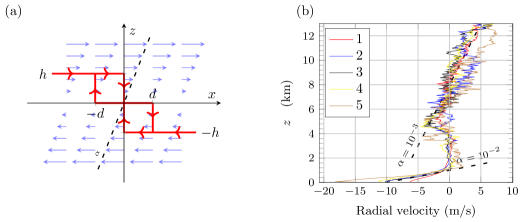
Figure 1: Left: flowfield model (thin arrows) and the three-level control (TLC) rule (thick lines). Right: radial velocity profiles, composite from dropsonde measurements between 1996 and 2012 within $200\text{\,}\mathrm{km}$ of the hurricane center (Wang et al.,, 2015), binned into $50\text{\,}\mathrm{m}$ altitude intervals and sorted according to hurricane category (1 to 5). The jaggedness of the profiles above $2\text{\,}\mathrm{km}$ altitude is due to the reduced number of available measurements with respect to the lower region. Dashed lines estimate the mean velocity gradient $\alpha$.

Rather than constraining the problem by the state-space representation of the system (2), as is done in (1), we thus instead use an equivalent condition on the PDF $p_{X,Z}(x,z)$, and restate the optimization problem (1) as

$$\min_{u}\; \mathbf{E}\left[\,|\bm{u}|\,\right]$$ (3a)

with $$\left\{\begin{matrix}\mathbf{E}\left[\left(\bm{X-\bar{X}}\right)^{2}\right]=\text{constant}\\[8.00003pt] \partial_{t}p_{\bm{X}}+\bm{f}(\bm{X},\bm{u})\cdot\nabla p_{\bm{X}}+\dfrac{c^{2}}{2}\nabla^{2}p_{\bm{X}}=0,\end{matrix}\right.$$ (3b)

where we have replaced the state equation in (1b) with an equivalent Fokker-Plank equation for the PDF $p_{\bm{X}}(\bm{x})$ (Risken,, 1984), and the norms are interpreted as expected values. The solution of the optimization problem as stated in (3) is the principal contribution of this work.

The remainder of this paper is concerned with the solution of the optimization problem (3) for the TLC rule of Figure 1a, and with comparison to the classical linear control rule $u=k_{1}x+k_{2}z$, whose optimal solution is given by the Linear Quadratic Regulator (LQR) Lewis and Syrmos, (1995). To facilitate comparison, we first derive the functional form of the solution by dimensional analysis.

II Dimensional analysis

The control problem is governed by three parameters: the velocity gradient $\alpha$, the spectral density $c^{2}$, and the target horizontal variance $\bar{\sigma}^{2}_{X}$. Take the length, time, and velocity scales as $L=\sqrt{c^{2}/\alpha}$, $T=\alpha^{-1}$, and $U=L/T=\sqrt{c^{2}\alpha}$. A single dimensionless parameter can be defined as

$$R={\bar{\sigma}_{X}^{2}\alpha}/{c^{2}},$$ (4)

and the dimensionless control cost can be written as $w/U~{}=\mathbf{E}\left[\,|u|\,\right]/U~{}=~{}\mathcal{F}(R)$ where $\mathcal{F}(R)$ is an unknown dimensionless function. Similar expressions can be written for $d/L$ and $h/L$. The system (2) is additionally invariant with respect to a rescaling of the vertical coordinate by the time scale $\alpha^{-1}$, thus reducing the parameters governing the problem to the standard deviation $\bar{\sigma}_{X}$ and the spectral density $c^{2}$. Dimensional analysis (Barenblatt,, 1996) can then be used to write the control cost as

$$\dfrac{w}{U}=\gamma_{w}\dfrac{1}{U}\dfrac{c^{4}}{\alpha\sigma_{X}^{3}}=\gamma_{w}\,R^{-\frac{3}{2}}.$$ (5)

Expressions for the control parameters can also be obtained as

$$\dfrac{d}{L}=\gamma_{d}\dfrac{\sigma_{X}}{L}=\gamma_{d}R^{\frac{1}{2}},\quad\dfrac{Z}{L}=\gamma_{h}\dfrac{1}{L}\dfrac{c^{2}}{\alpha\sigma_{X}}=\gamma_{h}R^{-\frac{1}{2}}.$$ (6)

The solution is then summarized by the optimal value of $\gamma_{(\cdot)}$ for each control parameter. Similarly, for the linear feedback control rule $u=k_{1}x+k_{2}z$, we can write $Tk_{1}=\gamma_{k_{1}}R^{-2}$ and $Tk_{2}=\gamma_{k_{2}}R^{-1}$. Note that the solution (5) is independent of the specific choice of the control rule $u(x,z)$; a comparison between different rules can be obtained by comparing the respective values of $\gamma_{w}$.

III Three-level control (TLC) rule

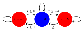
Figure 2: Implementation of the three-level control rule.

We now proceed in seeking the optimal values for the parameters $d$ and $h$ [equivalently, $\gamma_{d}$ and $\gamma_{h}$ in (6)] in the TLC rule indicated by thick lines in Figure 1a, corresponding to step changes in altitude $h$ at $x=0,\pm d$. In this limit, the governing equations (2) can be restated as

$$\dot{X}=-\alpha\bar{Z}+\xi,$$ (7)

where $X\in\mathcal{R}$ is the same as in the original problem, but $\bar{Z}\in\left\{-h,0,h\right\}$ is now a discrete rather than a continuous random variable, and the corresponding equation is replaced by the automata in Figure 2. This is a valid approximation when the control velocity $u$ is larger than the horizontal velocity scale $\sqrt{c^{2}\alpha}$. Note that the dynamics of (7) is quite simple, and is dominated by the effect of the stochastic excitation by $\xi$.

Let $p_{X,\bar{Z}}\left(x,\bar{z}\right)$ be the PDF of the balloon position, and $p_{\bar{z}}(x)=p_{X|\bar{Z}}\left(x|\bar{z}\right)\,p_{\bar{Z}}(\bar{z})$, so that $p_{X}(x)=\sum_{\bar{z}}p_{\bar{z}}(x)$ is the marginal probability. The governing equations for the PDFs can be written as

$$\begin{aligned} \partial_{t}p_{\bar{z}}(x)+\partial_{x}\alpha\bar{z}\,p_{\bar{z}}(x)-\partial_{xx}\dfrac{c^{2}}{2}p_{\bar{z}}(x)=0&\\ \textrm{for}\quad\bar{z}\in\{\!&-\!h,0,h\},\end{aligned}$$ (8a)

$$\left.\partial_{x}p_{X}(x)\right|_{x^{-}}=\partial_{x}\left.p_{X}(x)\right|_{x^{+}}\quad\textrm{for}\quad x\in\{-d,0,d\},$$ (8b)

where (8a) are three Fokker-Plank equations for each discrete altitude $\bar{z}$ obtained by considering the transition probabilities implied by (7), and (8b) represent the transition probabilities in the $z$ direction, and imposes the conservation of the probability fluxes represented by arrows in Figure 2. Equations (8) now take the role of the optimization problem constraint (3b).

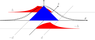
Figure 3: Steady state probability distribution functions for $c^{2}=h=\alpha=1$. Filled: $p_{0}(x)$ and $p_{\pm h}(x)$. Solid: marginal probability $p_{X}(x)=p_{0}(x)+p_{+h}(x)+p_{-h}(x)$. Dashed: normal distribution with the same variance.

The statistically steady-state solution of (8a) can actually be computed analytically, as shown in Figure 3, and is given by

$$p_{0}\left(x\right) =\left\{\begin{array}[]{ll}c_{1}x+c_{2}&\qquad\qquad 0<x<d,\\[10.00002pt] 0&\qquad\qquad d<x<\infty,\end{array}\right.$$ (9c)

$$p_{h}\left(x\right) =\left\{\begin{array}[]{ll}q_{1}\frac{\lambda}{2}\;e^{-\frac{2x}{\lambda}}+q_{2}&\quad 0<x<d,\\[10.00002pt] r_{1}\frac{\lambda}{2}\;e^{-\frac{2x}{\lambda}}+r_{2}&\quad d<x<\infty,\end{array}\right.$$ (9f)

where $\lambda=\frac{c^{2}}{gh}$ is twice the e-folding scale of the PDF (the symmetry of the problem at $x=0$ can be used to compute the solution for $x<0$, $\bar{Z}=h$). The integration constants $c_{1},c_{2},q_{1},q_{2},r_{1},r_{2}$ can be obtained imposing (8b) together with the boundary conditions $p_{0}(x=d)=0$, $p_{h}(x=0)=0$, $\lim_{x\rightarrow\infty}p_{X}(x)=0$, and the normalization condition $\int_{-\infty}^{\infty}p_{X}(x)dx=1$, resulting in

$$c_{1} =-\dfrac{1}{d(d+\lambda)},\ \ q_{1} =-\dfrac{1}{d(d+\lambda)},\ \ r_{1} =\dfrac{e^{\frac{2d}{\lambda}}-1}{d(d+\lambda)},$$

$$c_{2} =\dfrac{1}{d+\lambda}, q_{2} =\dfrac{\lambda}{2d(d+\lambda)}, r_{2} =0.$$ (10)

Upon substitution of the coefficients (10) into the expressions for $p_{0}$ and $p_{h}$ in (9), the variance can be written

$$\sigma_{X}^{2}=\int_{-\infty}^{\infty}x^{2}p_{X}(x)dx=\dfrac{d^{3}+2\lambda d^{2}+3\lambda^{2}d+3\lambda^{3}}{6(d+\lambda)}.$$ (11)

The control cost can be computed as the total transition probability between the states $\bar{Z}=0$ and $\bar{Z}=h$, multiplied by the cost of the single control activation $h$:

$$w=2\alpha hc^{2}\left.\partial_{x}p_{0}\right|_{x=d}=\dfrac{2ghc^{2}}{d(d+\lambda)}.$$ (12)

The control parameters $h$ and $d$, and the corresponding control cost $w$, can then be computed by minimization of the objective functional (3a). The corresponding dimensionless constants in (5) and (6) are

$$\gamma_{w}=0.5432,\quad\gamma_{d}=1.6288,\quad\gamma_{h}=1.1166,$$ (13a)

$$f=0.4864\,{c^{2}}/{\sigma_{x}^{2}}=0.4864\,T^{-1}\,R^{-1},$$ (13b)

where $f$ is the frequency at which the control has to be activated, and can be computed by considering the times $t_{out}=d^{2}/c^{2}$ and $t_{in}=d/(gZ)$ to reach the location $x=d$ from $x=0$ and back, respectively.

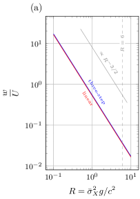
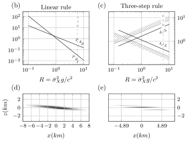
Figure 4: Comparison of control rules: (a) control cost $w=\mathbf{E}\left[\,|u|\,\right]$ as a function of the dimensionless parameter $R$ for the two different control rules; the two control costs are almost indistinguishable, differing by less than $5\%$. (b,c) Control parameters and (d,e) corresponding probability density for the hurricane case $(R=6)$ for the linear and TLC control rules; gray patterns in (c) define the limit of each curve for which a given value of $R$ is attainable, given by (14).

It is also of interest to compute the minimum variance attainable for given values of $d$ and $h$, and from there obtain the limiting values of $d$ and $h$ for a specified $\bar{\sigma}_{X}$:

$$\lim_{h\rightarrow\infty}\sigma_{X}^{2}=\dfrac{d^{2}}{6} \quad\Rightarrow\quad d<\sqrt{6}\,\bar{\sigma}_{X},$$ (14a)

$$\lim_{d\rightarrow 0}\sigma_{X}^{2}=\dfrac{c^{4}}{2\alpha^{2}h^{2}} \quad\Rightarrow\quad h>\dfrac{1}{\sqrt{2}}\dfrac{c^{2}}{\bar{\sigma}_{X}\alpha}.$$ (14b)

In both limits the control cost tends to infinity, in the first case because $h\rightarrow\infty$, and in the second because the frequency of the steps increases without bound. Reasonable (finite) values of $h$ and $d$, away from these limiting values, are thus important in application. Results are summarized in Figure 4.

IV Application to the control of balloons within a hurricane

Finally, we compute optimal values of the control parameters for atmospheric balloons within an idealized hurricane flowfield, and compare them with results using the linear control rule $u=k_{1}x+k_{2}z$. A velocity gradient of $\alpha=${10}^{-3}\text{\,}{\mathrm{s}}^{-1}$$ (see Figure 1b) and a spectral density of $c^{2}=$1500\text{\,}{\mathrm{m}}^{2}\text{\,}{\mathrm{s}}^{-1}$$ (Zhang and Montgomery,, 2012) are assumed.

We additionally impose a target standard deviation of $\bar{\sigma}_{X}=$3\text{\,}\mathrm{k}\mathrm{m}$$, resulting in $R=6$ [see (4)]. Control parameters and control cost can be obtained using (6) together with the values in (13). For the TLC rule,

$$d =$4886.4\text{\,}\mathrm{m}$,\quad h =$558.3\text{\,}\mathrm{m}$,$$ (15a)

$$w =$4.54\text{\times}{10}^{-2}\text{\,}\mathrm{m}\mathrm{/}\mathrm{s}$,\quad f =$8.11\text{\times}{10}^{-5}\text{\,}\mathrm{s}^{-1}$,$$ (15b)

where $f$ corresponds to a period of about 3.5 hours.

The optimal solution for the linear control rule can be readily obtained by solving (1), resulting in

$$k_{1} =$3.125\text{\times}{10}^{-5}\text{\,}\mathrm{s}^{-1}$,\quad k_{2} =$2.5\text{\times}{10}^{-4}\text{\,}\mathrm{s}^{-1}$,$$ (16a)

$$w =$4.32\text{\times}{10}^{-2}\text{\,}\mathrm{m}\mathrm{/}\mathrm{s}$.\qquad$$ (16b)

Simulations for both control rules are shown in Figure 4d and 4e.

V Conclusions

This paper introduces a probabilistic framework for the optimization of physical systems dominated by stochastic excitation in the presence of mixed continuous and discrete random variables, non-linearities, and hysteresis. Its application has been demonstrated by addressing the problem of controlling atmospheric balloons within a stratified flowfield; the same framework can be extended to a class of problems that, to the authors’ knowledge, were previously intractable from an optimization point of view. From an application perspective, the three-level control (TLC) rule of Figure 2 has many advantages: holding rather than continuously adjusting a position is often an easier solution to implement, possibly requiring less energy in real life applications. For an observational platform like a sensor balloon, it has the additional advantage of performing measurements which are not disturbed by continuous control actions.

References

- Barenblatt, (1996) Barenblatt, G. I. (1996). Scaling, self-similarity, and intermediate asymptotics: dimensional analysis and intermediate asymptotics, volume 14. Cambridge University Press.
- Lewis and Syrmos, (1995) Lewis, F. L. and Syrmos, V. L. (1995). Optimal control. John Wiley & Sons.
- Nocedal and Wright, (2006) Nocedal, J. and Wright, S. (2006). Numerical optimization. Springer Science & Business Media.
- Risken, (1984) Risken, H. (1984). Fokker-planck equation. In The Fokker-Planck Equation, pages 63–95. Springer.
- Wang et al., (2015) Wang, J., Young, K., Hock, T., Lauritsen, D., Behringer, D., Black, M., Black, P. G., Franklin, J., Halverson, J., Molinari, J., et al. (2015). A long-term, high-quality, high-vertical-resolution GPS dropsonde dataset for hurricane and other studies. Bulletin of the American Meteorological Society, 96(6):961–973.
- Zhang and Montgomery, (2012) Zhang, J. A. and Montgomery, M. T. (2012). Observational estimates of the horizontal eddy diffusivity and mixing length in the low-level region of intense hurricanes. Journal of the Atmospheric Sciences, 69(4):1306–1316.