The double galaxy cluster Abell 2465 III. X-ray and weak-lensing observations

Abstract

We report Chandra X-ray observations and optical weak-lensing measurements from Subaru/Suprime-Cam images of the double galaxy cluster Abell 2465 ($z=0.245$). The X-ray brightness data are fit to a $\beta$-model to obtain the radial gas density profiles of the northeast (NE) and southwest (SW) sub-components, which are seen to differ in structure. We determine core radii, central temperatures, the gas masses within $r_{\mathrm{500c}}$, and the total masses for the broader NE and sharper SW components assuming hydrostatic equilibrium. The central entropy of the NE clump is about two times higher than the SW. Along with its structural properties, this suggests that it has undergone merging on its own. The weak-lensing analysis gives virial masses for each substructure, which compare well with earlier dynamical results. The derived outer mass contours of the SW sub-component from weak lensing are more irregular and extended than those of the NE. Although there is a weak enhancement and small offsets between X-ray gas and mass centers from weak lensing, the lack of large amounts of gas between the two sub-clusters indicates that Abell 2465 is in a pre-merger state. A dynamical model that is consistent with the observed cluster data, based on the FLASH program and the radial infall model, is constructed, where the subclusters currently separated by $\sim 1.2$ Mpc are approaching each other at $\sim 2000$ km s^-1and will meet in $\sim 0.4$ Gyr.

1. Introduction

In the $\Lambda$ cold dark matter ($\Lambda$CDM) picture of large-scale structure formation, galaxy clusters grow hierarchically from smaller knots of higher density forming and merging along the intersection of filaments. Examples of interacting clusters that have undergone merging interactions include e.g. the ’Bullet’ (Clowe et al. 2006), RXJ1347.5-1145, (Bradač et al. 2008a), MACSJ0025.4-1222 (Bradač et al. 2008b), Abell 2744 (Owers et al. 2011), Abell 2146 (Russell et al. 2012), and DLSCL J00916.2+2915 (Dawson et al. 2012). Some examples of pre-collisional binary clusters include Abell 3716 (Andrade-Santos et al. 2015) and Abell 1750 and 1758 (Okabe & Umetsu 2008). Other possible objects have been given in Hwang & Lee (2009)and Molnar et al. (2013) In X-rays, the structures of the gas in galaxy clusters can be compared with the other components and this indicates a range of structures extending from circular symmetry, indicating relaxed objects, to separated and disturbed gas indicating core-crossing events ranging from pre- to post-mergers (e.g. Markevitch & Vikhlinin 2007).

Modelling cluster collisions indicates the different behavior of the collisionless dark matter and baryonic gas constituents (e.g. Roettiger et al. 1997; Takizawa 2000; Ricker & Sarazin 2001; Poole et al. 2006; Molnar, Hearn, & Stadel 2012). Several investigators (e.g. Spergel & Steinhardt 2000; Kahlhoefer et al. 2014) have proposed utilizing these effects to study nongravitational interactions of dark matter in the collisions of the galaxy clusters to gain information on the properies of the dark matter component. Vijayaragharan & Ricker (2013) have shown that these effects begin to be felt even in the pre-merger phases so details of the dynamics at all stages of cluster mergers provide rich information about the physical interplay between dark matter and baryons.

Investigating double galaxy clusters by combining optical, radio, and X-ray data with gravitational lensing provides insight into the star formation and the evolution of of these clusters and ultimately large-scale structure. Weak lensing is a powerful tool for reconstructing cluster mass distributions on large angular scales and for identifying mass substructures (Okabe & Umetsu 2008; Medezinski et al. 2013; Umetsu et al. 2012). In many cases, the substructure of galaxy clusters complicates their interpretation if they have many components (e.g. Cohen et al. 2014; Merten et al. 2011; Medezinski et al. 2016) and consequently finding simple clearly double structures is valuable for elucidating the dynamics of their components.

Abell 2465 appears to be a well defined double cluster system undergoing a major merger. First reported by Abell (1958) as a modest Richness Class 1 cluster, its double nature was not known until Vikhlinin et al. (1998) gave ROSAT X-ray fluxes of the two sub-components, referred to in this paper as the northeast (NE) and southwest (SW) components (See Figure 1). Perlman et al. (2002) found redshifts of $z=0.245$ for both, establishing their physical relationship. The NE component of the cluster is detected in the FIRST 1.4 Ghz survey (Condon et al. 1998; Helfand, White, & Becker 2015).

The optical properties of Abell 2465 have been described in Wegner (2011; Paper I) and Wegner, Chu, & Hwang (2015; Paper II). Virial masses $M_{\mathrm{vir}}=(4.1\pm 0.8)\times 10^{14}M_{\odot}$ and $(3.8\pm 0.8)\times 10^{14}M_{\odot}$ (all relevant symbols are defined at the end of this section) for NE and SW respectively were derived from optical velocity dispersions. Although they have similar masses, the two subclusters differ in their radial profiles. The NE is less compact, while the SW is smaller in extent with a brighter inner core. In Paper II, it was found that star formation rates of member galaxies appear enhanced. Since the projected separation between the two subclusters is 1.2 Mpc and their optical halo radii are $r_{\mathrm{200c}}\approx 1.2$ and $1.25$ Mpc (Paper I), detectable effects of their interaction seem possible.

To look for such effects, we obtain and analyze new Chandra X-ray observations and weak-lensing measurements from Subaru Suprime-Cam imaging. These are utilized to determine the state of the baryonic gas and measure the structures and mass distibutions of the double components of Abell 2465, study their interaction, and settle whether they are pre- or post-core crossing.

This paper is arranged as follows: Section 2 discusses the X-ray data. Section 2.1 presents the Chandra observations and reductions. Section 2.2 analyzes the X-ray spatial and spectral data and the resulting total and gas masses for the NE and SW subclusters. Section 2.3 determines the gas temperaures of the substructures and Section 2.4 derives the individual entropies. Section 2.5 describes the search for gas between the subclusters. Section 2.6 further presents the optical appearances of the components. Section 3 contains the optical imaging data and weak-lensing results for Abell 2465. Section 3.1 covers the observations, Sections 3.2 and 3.3 explain the shape measurements and background selection for the weak-lensing analysis. Multi-halo mass modeling is in Section 3.4. Section 4 concerns the dynamical state of and modeling of Abell 2465. Section 5 discusses these results and how the cluster compares with other merging galaxy clusters. Section 6 lists our conclusions.

We assume a standard $\Lambda$CDM cosmology with $\Omega_{\mathrm{m}}=0.3$, $\Omega_{\Lambda}=0.7$, and $H_{0}=100h$ km s^-1 Mpc^-1 with $h=0.7$. For the cluster’s mean redshift, $z=0.245$, the luminosity distance is $D_{L}=1224$ Mpc and the scale on the sky is 230 kpc arcmin^-1. The two subclusters are separated by 5.25 arcmin or 1.2 Mpc.

We use the standard notation $M_{\Delta\mathrm{c}}$ to denote the mass enclosed within a sphere of radius $r_{\Delta\mathrm{c}}$, within which the mean overdensity is $\Delta_{\mathrm{c}}$ times the critical density $\rho_{\mathrm{c}}$ of the universe at the cluster redshift. To calculate halo virial quantities, we use an expression for the virial overdensity $\Delta_{\mathrm{vir}}$ based on the spherical collapse model (see Appendix A of Kitayama & Suto 1996).

2. Properties if Abell 2465 from X-ray observations

2.1. Chandra X-ray Data

Abell 2465 was observed 2012 October 6 and 2 in the 0.1-10 keV energy range with the ACIS-I detectors of Chandra, ObsIds 14010 and 15547 for 40 ks and 30 ks respectively. Both the NE and SW sub-components were well placed together across the instrument. With Chandra , about 1800 net counts were collected from each sub-cluster after background subtraction. Data reductions applied CALDB 4.6.7 and followed Vikhlinin et al. (2005). The reductions used the Chandra Interactive Analysis of Observations (CIAO) package and included calibration corrections to the individual photons, calibration of the spectral response, background subtraction including quiescent and soft background correction, and subtraction of the readout artifacts. We reprocessed the data, excluded flare contaminated time intervals, detected and excluded point sources, merged the data sets, utilized ACIS blank sky observations to subtract the background, and removed readout artifacts.

Although XMM-Newton images of Abell 2465 are available (Paper I), we only utilize the newer Chandra observations. Both data sets have similar number counts, but the cluster falls at the edge of the serendipitous XMM-Newton field of view which badly degrades the point spread function and renders these data unsuitable for point source removal and producing surface brightness, emission measure, and gas mass profiles.

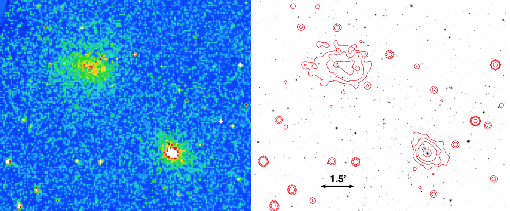
Figure 1.— Left: Chandra image of Abell 2465 in the 0.5 to 3.0 keV energy band with 8 pixel binning. Right: CFHT megaprime $i^{\prime}$ image with the isodensity X-ray contours. North is to the top and West to the right. The images are approximately $11\times 9$ arcmin². The NE component is to the upper left and comparison with the SW component shows the differences in their structures. The X-ray center of the NE sub-cluster is slightly displaced from its central BCGs while the SW X-ray peak is nearly centered on the BCG.

Figure 1 presents both the resulting Chandra image and its isodensity contours overlaying the optical $i^{\prime}$ image from the 3.6 m Canada–France–Hawaii Telescope (CFHT; see Section 3.1). This shows the different appearances of the two sub-clusters. The X-ray profile of the NE component, although it is the more massive and luminous, has a broad central maximum. It has two X-ray concentrations oriented E and W. The SW peak is the brighter and is not near a radio or optical source. The NE peak coincides with with a FIRST Survey radio source (Condon 1998; Helfand et al. 2015) and an optical brightest cluster galaxy (BCG). It is significantly offset from the X-ray center of the NE clump. The BCG consists of at least three merging ellipticals and has no detected optical emission lines (Paper I and Figure 5). The NE subcluster is itself, likely the result of a merger. The SW component is more compact and shows a brighter sharp central peak. A cool core was suggested as possible in Paper I. The BCG in the SW clump also shows no optical emission lines. A further comparison of the optical and X-ray appearances of the two components is given in Section 2.6.

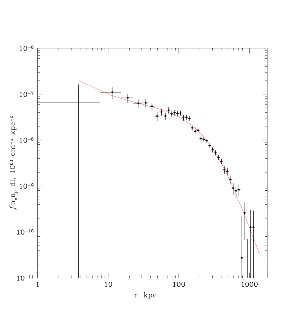
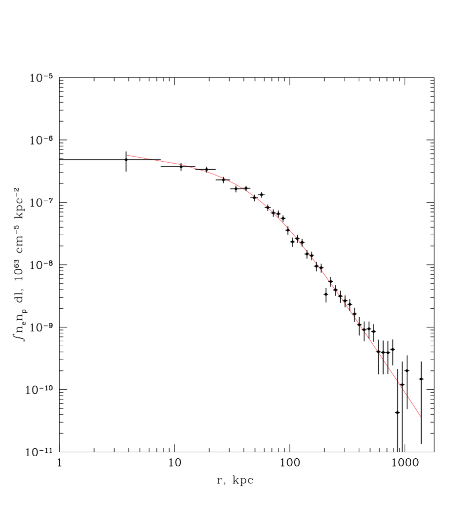
Figure 2.— Emission measure profiles for the NE (left) and SW (right) subclusters of Abell 2465 showing the Chandra measurements and their error bars with the resulting model fits from Eq. (1).

2.2. The X-ray radial brightness and gas density profiles of Abell 2465 NE and SW

The projected X-ray surface brightness distributions of the two components of Abell 2465 were measured, from which the total X-ray luminosities were found to be: $L_{X,\mathrm{bol}}=9.0^{+0.3}_{-0.5}\times 10^{43}$ erg s^-1 for the NE component and $L_{X,\mathrm{bol}}=6.8^{+0.2}_{-0.3}\times 10^{43}$ erg s^-1 for the SW component, comparable to the results in Paper I from XMM-Newton and ROSAT data.

Assuming spherical symmetry, inverting Abel’s integral, yields the emission measure, $\epsilon_{\nu}$, from which results the particle densities, $n_{p}n_{e}=\epsilon_{\nu}/\Lambda(T_{\mathrm{g}})$ of each subcluster, where $\Lambda(T_{\mathrm{g}})$ describes the emissivity of the gas at temperature $T_{\mathrm{g}}$.

The modified $\beta$ model (Vikhlinin et al. 2006) which fits the emission measure profiles of a wide range of clusters was used:

$$n_{p}n_{e} = n_{0}^{2}\frac{(r/r_{\mathrm{c}})^{-\alpha}}{[1+(r/r_{\mathrm{c}})^{2}]^{3\beta-\alpha/2}}\frac{1}{[1+(r/r_{\mathrm{s}})^{\gamma}]^{\epsilon/2}}$$ (1)

$$+\frac{n_{02}^{2}}{[1+(r^{2}/r_{\mathrm{c2}})^{2}]^{3\beta_{2}}},$$

where $n_{0}$ the central number density, $\beta$, and $r_{\mathrm{c}}$ the core radius have their usual meanings. The additional parameters, $\epsilon$, $r_{\mathrm{s}}$, and $\gamma$ account for a slope change and the slope width transition. A second small $\beta$ profile with parameters $n_{02},r_{\mathrm{c2}},$ and $\beta_{2}$ is added. The resulting emission measure profiles of both subclusters and the fits to (1) are shown in Figure 2. Table 1 gives the best fit parameters for the $\beta$-model for the NE and SW clumps. This confirms the visual impression of the differences between the two, where the core radius, $r_{\mathrm{c}}$, of the NE component is nearly $5\times$ larger than that of its SW neighbor.

Table 1Chandra emission measure model best fits (Eq. [1])

Sub-	$n_{0}$	$r_{\mathrm{c}}$	$r_{\mathrm{s}}$	$\alpha$	$\beta$	$\gamma$	$\epsilon$	$n_{02}$	$r_{\mathrm{c2}}$	$\beta_{2}$
component	($10^{-3}$ cm-3)	(kpc)	(kpc)					(cm-3)	(kpc)
A2465 NE	1.578	337	388	0.719	0.849	0.500	0.456	$3.55\times 10^{-2}$	3.37	0.502
A2465 SW	10.763	62	64	0.693	0.543	0.577	0.645	$7.09\times 10^{-6}$	2.03	0.503

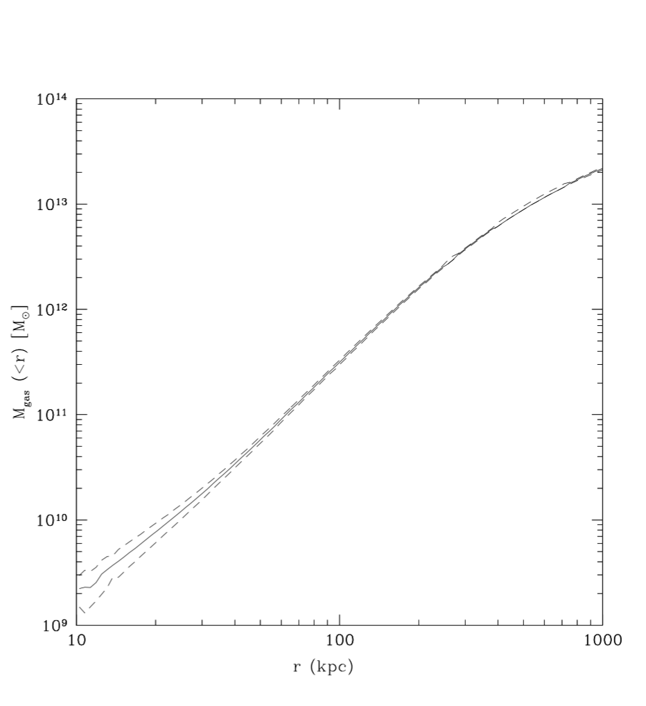
Figure 3.— Enclosed gas mass $M_{\mathrm{g}}(<r)$ profiles for Abell 2465 NE (left) and SW (right). Dashed curves indicate $1\sigma$ or 68% confidence levels.

Table 2Fitted $\beta$-model parameters and central density

Sub-	$r_{\mathrm{c}}$	$\beta$	$n_{0}$	$\rho_{0}$(10 kpc)	$M_{\mathrm{hyd}}$	$r_{\mathrm{500c}}$	$M_{\mathrm{g}}$
component	(kpc)		(10-3 cm-3)	($10^{-3}$ g cm-3)	($10^{14}M_{\odot}$)	(kpc)	($10^{13}M_{\odot}$)
A2465 NE	$337\pm 45$	$0.85\pm 0.11$	$1.578\pm 0003$	$9.0\pm 3.3$	1.85${}^{+0.60}_{-0.40}$	696${}^{+75}_{-50}$	1.90${}^{+0.05}_{-0.04}$
A2465 SW	$62\pm 11$	$0.54\pm 0.03$	$10.763\pm 0.002$	$18.5\pm 3.1$	$2.17\pm 0.22$	731$\pm 25$	$0.96\pm 0.03$

The gas mass of each subcluster

$$M_{\mathrm{g}}=4\pi\int^{r_{\mathrm{500c}}}_{0}\rho_{\mathrm{g}}(r)r^{2}dr$$ (2)

within $r_{\mathrm{500c}}$, the spherical radius where the mean density, $\bar{\rho}=500\rho_{\mathrm{c}}$, with $\rho_{\mathrm{c}}$ the critical density at the cluster’s redshift, $z=0.245$ was determined using (1) and equation (4) in Andrade-Santos et al. (2015) for the central electron density, $n_{e,0}$ for a plasma with fixed electron to hydrogen density, $n_{e}/n_{H}$, inside a ring of given inner and outer radii, then $\rho_{\mathrm{g}}=\mu_{e}n_{e}m_{p}$ where $\mu_{e}=1.17$ is the electron mass molecular weight and $n_{e}/m_{H}=1.2$.

The 3D gas densities and temperature profiles are used to calculate the total masses, $M_{\mathrm{hyd}}(<r)$, inside a clusterc radius, $r$ assuming hydrostatic equilibrium and a metal abundance for the gas of $0.3Z_{\odot}$,

$$M_{\mathrm{hyd}}(<r)=-3.67\times 10^{13}M_{\odot}kTr\Big{(}\frac{d\ln\rho_{\mathrm{g}}}{d\ln r}+\frac{d\ln T}{d\ln r}\Big{)},$$ (3)

(e.g. Sarazin 1986; Andrade-Santos et al. 2015), where $k$ is the Boltzmann constant, $T$ is the gas temperature in K, and $r$ is in Mpc.

The $M_{\mathrm{hyd}}(<r)$ is used to obtain $r_{\mathrm{500c}}$ from

$$M_{\mathrm{hyd}}(<r_{\mathrm{500c}})=500\rho_{\mathrm{c}}(4\pi/3)r_{\mathrm{500c}}^{3}.$$ (4)

Table 3Temperature Measurements in Abell 2465

Component	$r$ (kpc)	$kT$ (keV)	Component	$r$ (kpc)	$kT$ (keV)
NE core	0 - 134	$3.38^{+0.42}_{-0.28}$	SW core	0 - 77	$2.77^{+0.21}_{-0.18}$
NE periphery	134 - 326	$3.55^{+0.46}_{-0.41}$	SW periphery	77 - 287	$2.48^{+0.24}_{-0.23}$

Table 2 gives the best fitting parameters for $M_{\mathrm{hyd}},M_{\mathrm{g}}$, $r_{\mathrm{c}}$ and $\beta$ from the combined data plus the central values of the electron density and the mass density. Within $r_{\mathrm{500c}}$, the two clusters have nearly equal $M_{\mathrm{hyd}}$. The NE cluster has the higher gas content ($\sim 2\times M_{\mathrm{g}}/M_{\mathrm{hyd}}$) due to its larger core radius and at $r_{\mathrm{200c}}$ it has the stronger $L_{X}$ and $M_{\mathrm{200c}}$.

2.3. Gas temperatures in Abell 2465

The gas temperature of the sub-clusters could only be extracted near their centers. With Chandra , about 1800 net counts were collected from each sub-cluster. For the NE subcluster, a circle (0–35) arcsec corresponding to (0–134) kpc was used; the corresponding area for the SW component was (0–20) arcsec or (0–77) kpc. Data in the 0.6–10 keV band were fit to an apec single temperature model (Smith et al. 2001). The metallicity was assumed to be $0.3Z_{\odot}$. The absorption correction was obtained from the $N_{H}$ value from radio surveys (Dickey & Lockman 1990). The central temperatures are given in Table 3. Noting the difference in their brightness profiles, the NE subcluster has the higher temperature indicative of a non-cool core, while the lower temperature of the more centrally concentrated SW component suggests a cool core.

2.4. Entropy of the two sub-clusters

The entropy provides information on a galaxy cluster’s history (Voit et al.  2005; McDonald et al.  2013; Andrade-Santos et al.  2015). As the temperature profiles in Abell 2465 cannot be determined, the entropy is limited to the central regions, within radii 0-20 arcsec.

The specific entropy is $K=kT/n_{e}^{2/3}$, with $k$ the Boltzmann constant, $T$ the temperature of the intercluster gas, and $n_{e}$ the electron density. The central entropies are found to be $K=78\pm 21$ keV cm² for the NE component and $K=40\pm 5$ keV cm² for the SW component. For the SW sub-cluster, $K$ is consistent for a $T\sim 3$ keV relaxed cluster where $K_{0}\sim 10-30$ keV cm² (Voit et al. 2005; Cavagnolo et al. 2009; McDonald et al. 2013), for the NE component, $K_{0}$ is a factor of $\sim 2$ higher.

The reduced entropy relation predicted from purely gravitational heating is (Pratt et al. 2010),

$$K/K_{\mathrm{500c}}=1.42(r/r_{\mathrm{500c}})^{1.1}$$ (5)

where $K_{\mathrm{500c}}=106[(M_{\mathrm{500c}}/10^{14}M_{\odot})/f_{\mathrm{b}}/E(z)]^{\frac{2}{3}}$ KeV cm^-2. For both components of Abell 2465, $M_{\mathrm{500c}}\approx 2\times 10^{14}M_{\odot}$. With a baryon fraction $f_{\mathrm{b}}\approx 0.15$, $r_{\mathrm{500c}}\approx 0.7$ Mpc, and $E(z)=1.131$, $K_{\mathrm{500}}\approx 550$ keV cm².

Galaxy mergers, AGN activity, or subcluster mergers might provide heating. Andrade-Santos et al. (2015) reviewed galaxy clusters with higher entropy showing signs of merging activity with two or more core ellipticals (e.g. Cavagnola et al. 2009; Seigar et al. 2003; and Wang, Owen, & Ledlow 2004). Pratt et al. (2010) show that $K/K_{\mathrm{500c}}$ divides the clusters roughly into two types which places the SW clump ($K/K_{\mathrm{500c}}\sim 0.07$) among cool core clusters while the NE ($K/K_{\mathrm{500c}}\sim 0.14$) lies with disturbed clusters. The NE clump may still be merging. In the optical, it has several BCGs shown below in Figure 5. A typical merger time is of order a Gyr (Seigar et al. 2003).

If a shock wave raised $K$ for Abell 2465 NE, the initial $K_{\mathrm{i}}$ to final $K_{\mathrm{f}}$ entropy ratio gives the order of magnitude of the required Mach number, $M=u/c_{\mathrm{s}}$, based on the Rankine-Hugoniot jump conditions (Andrade-Santos 2015; Belsole et al. 2004; Zel’dovich & Raizer 1967). If the NE component was initially relaxed, $K_{\mathrm{i}}\sim 25$ keV cm² then $K_{f}/K_{\mathrm{i}}\sim 1.6$ and $M\approx 3.28$. For $T\sim 3$ keV, $u\sim 2900$ km s^-1; compared to $(2GM_{\mathrm{200c}}/r_{\mathrm{200c}})^{\frac{1}{2}}\sim 3000$ km s^-1, the maximum collisional velocity expected for the clusters. This would seem possible if it were not for the lack of other collisional signs bridging the two components.

2.5. Search for inter-component gas and surface brightness jump

Enhanced gas density or surface brightness jumps between the components of Abell 2465 would be clues about the dynamical state of the merger. We constructed a surface brightness profile between the sub-clusters using the 0.5–2.0 keV Chandra image to maximize S/N employing the Proffit software package (Eckert, Molendi, & Paltani 2011). Boxes projected on the sky were $150\times 30$ arcsec with a $45\mbox{${}^{\circ}$}$ position angle, and span both sub-clusters including regions beyond them. The surface brightness profile in Figure 4 reveals a hot gas distribution virtually identical in both directions, with no visible enhancement between the two sub-clusters. No statistically significant sharp surface brightness (or density) jumps between the two clumps were detected, and no hint of elevated brightness between them, compared to the cluster outskirts, are detected at the signal-to-noise of the current data. We will carry out a quantitative analysis using numerical simulations in Section 4.

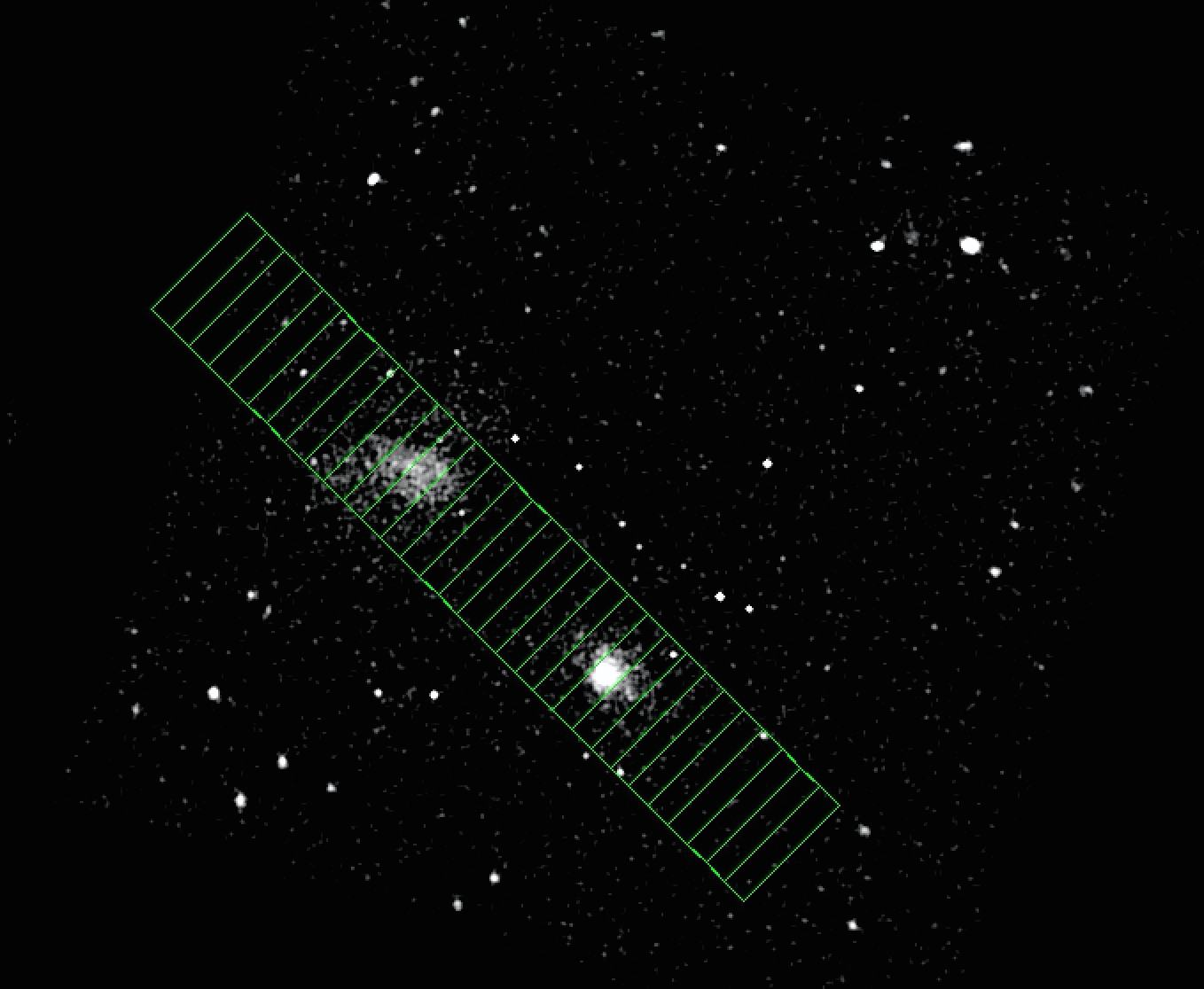
Figure 4.— Showing the absence of gas enhancement and sharp intensity jumps between the components of Abell 2465. Left: locations of bins on the Chandra (0.5–2.0) keV image; bins are $150\times 30$ arcmins. Right: surface brightness in the bins; NE sub-cluster is to the left and SW to the right. The peaks are 5.25 arcmin or 1.2 Mpc apart.

2.6. Optical appearance of the central BCG regions

Figure 5 shows the centers of the NE and SW components of Abell 2465 in the Subaru $Vi^{\prime}z^{\prime}$ image described in Section 3. In the NE clump, the light of the two central E galaxies seen in Figure 1 appears merged and connected to a third galaxy to the W and surrounded by at least three nearby E galaxies. The SW clump does not show such an extended distribution, but the large central BCG is associated with several close smaller galaxies to the north.

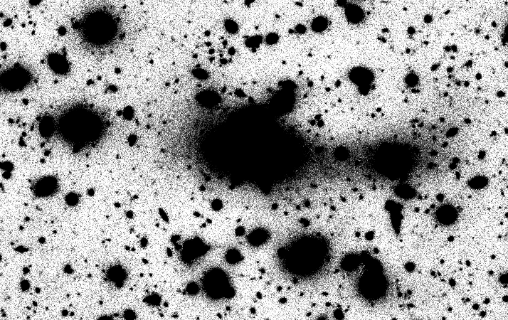
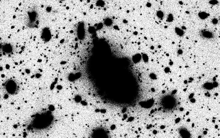
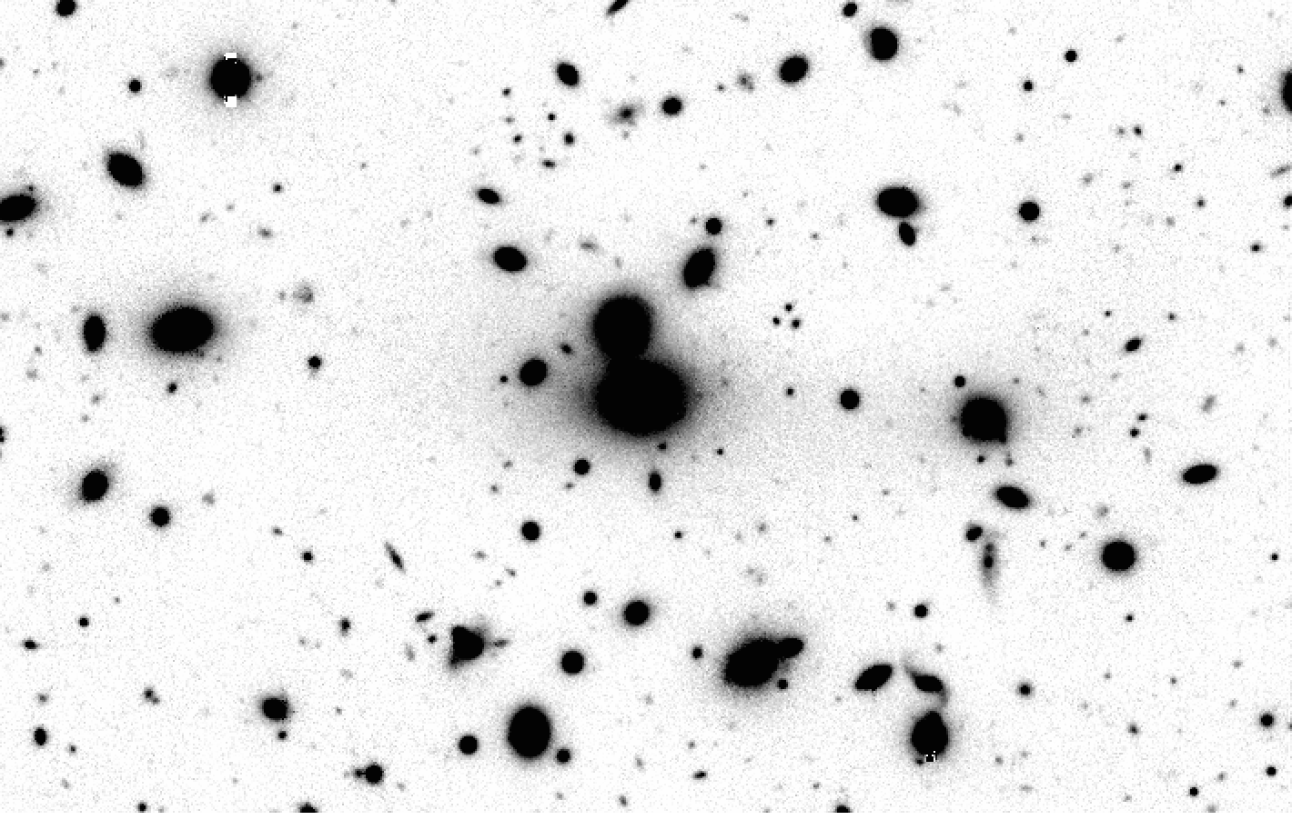
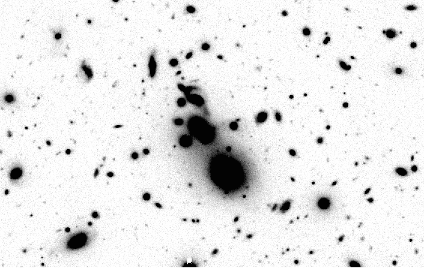
Figure 5.— The centers of the subcomponents of Abell 2465 from the combined Suprime-Cam $Vi^{\prime}z^{\prime}$ images described in Section 3 showing the BCGs. The NE (left) component and the SW (right) component are shown. North is to the top and west to the right. The vertical edge of each image is about 1.5 arcmin or 345 kpc. The top row shows faint details near the sky limit. The bottom row is set to bring out the peaks of the brightest objects.

3. Weak-lensing analysis

Our weak-lensing results are based on Subaru/Suprime-Cam images. The weak-lensing methodology has been described in our previous papers (see Umetsu & Broadhurst 2008; Umetsu et al. 2009, 2010, 2012, 2014; 2015; Medezinski et al. 2013, 2016). We therefore refer the reader to these papers and briefly outline the methodology here.

In this work, we study the projected mass distribution in the field of Abell 2465, $\kappa(\mbox{\boldmath$\theta$})=\Sigma(\mbox{\boldmath$\theta$})/\Sigma_{\mathrm{c}}$, which describes the projected mass density $\Sigma(\mbox{\boldmath$\theta$})$ in units of the critical surface density for lensing, $\Sigma_{\mathrm{c}}=(c^{2}D_{\mathrm{s}})/(4\pi GD_{\mathrm{l}}D_{\mathrm{ls}})=c^{2}/(4\pi GD_{\mathrm{l}}\beta)$, where $D_{\mathrm{l}},D_{\mathrm{s}},$ and $D_{\mathrm{ls}}$ are the angular diameter distances to the lens, the source, and the lens-source, respectively; $\beta(z,z_{\mathrm{l}})$ is the geometric lensing strength as a function of source redshift $z$ and lens redshift $z_{\mathrm{l}}$.

The complex gravitational shear field $\gamma(\mbox{\boldmath$\theta$})$ is nonlocally related to the convergence by $\partial^{*}\partial\kappa(\mbox{\boldmath$\theta$})=\partial^{*}\partial^{*}\gamma(\mbox{\boldmath$\theta$})$, where $\partial:=\partial/\partial\theta_{1}+i\partial/\partial\theta_{2}$ is a complex gradient operator that transforms as a vector, $\partial^{\prime}=\partial e^{i\phi}$, with $\phi$ the angle of rotation. In the subcritical regime where $(1-\kappa)^{2}-|\gamma|^{2}>0$, the reduced gravitational shear $g(\mbox{\boldmath$\theta$})=\gamma(\mbox{\boldmath$\theta$})/[1-\kappa(\mbox{\boldmath$\theta$})](<1)$ can be directly observed from a local ensemble of image ellipticities of background galaxies (e.g., Bartelmann & Schneider 2001).

In our weak-lensing analysis of the Abell 2465 field, we calculate the weighted average of reduced shear on a regular Cartesian grid of cells ($m=1,2,...,N_{\mathrm{cell}}$) as

$$\langle g(\mbox{\boldmath$\theta$}_{m})\rangle=\frac{\sum_{i}S_{i}(\mbox{\boldmath$\theta$}_{m}-\mbox{\boldmath$\theta$}_{i})w_{i}g_{i}}{\sum_{i}S_{i}(\mbox{\boldmath$\theta$}_{m}-\mbox{\boldmath$\theta$}_{i})w_{i}},$$ (6)

where $S(\mbox{\boldmath$\theta$})$ is a spatial window function, $g_{i}$ is the estimate for the reduced shear of the $i$th galaxy at $\theta_{i}$, and $w_{i}$ is the statistical weight for the $i$th galaxy,

$$w_{i}=\frac{1}{\sigma_{g,i}^{2}+\alpha_{g}^{2}},$$ (7)

with $\sigma_{g,i}^{2}$ the error variance of $g_{i}$ and $\alpha_{g}^{2}$ the constant variance taken to be $\alpha_{g}=0.4$, which is a typical value of the mean rms $\sqrt{\overline{\sigma^{2}}_{g}}$ found in Subaru observations (e.g., Umetsu et al. 2009, 2014; Okabe et al. 2010; Okabe & Smith 2016). The variance of the grid reduced shear is estimated by (Umetsu et al. 2009, 2015)

$$\sigma^{2}_{g}(\mbox{\boldmath$\theta$}_{m})=\frac{\sum_{i}S^{2}(\mbox{\boldmath$\theta$}_{m}-\mbox{\boldmath$\theta$}_{i})w_{i}^{2}\sigma_{g,i}^{2}}{\left(\sum_{i}S(\mbox{\boldmath$\theta$}_{m}-\mbox{\boldmath$\theta$}_{i})w_{i}\right)^{2}}.$$ (8)

3.1. Observational Data and Photometry

For the weak-lensing analysis, we use archived imaging from the Suprime-Cam ($34\arcmin\times 27\arcmin$; Miyazaki et al. 2002) at the prime focus of the 8.3 m Subaru telescope, where archived images were obtained from SMOKA . We also included observations from the CFHT/MegaCam. The CFHT/MegaCam $i^{\prime}$ and $r^{\prime}$ images have been describes in Paper I and also archived.

The imaging data are summarized in Table 4. The reduction procedure is based on Nonino et al. (2009) and further described in detail by Medezinski et al. (2013). We note that the present analysis used the CFHT imaging only for the catalog making and magnitude zero-point calibration.

Table 4 Optical imaging data of Abell 2465

Telescope	Filter	Exposure time	Seeing	$m_{\mathrm{lim}}$	Obs. Date
		(s)	(arcsec)	(AB mag)	yy/dd/mm
Subaru/S-Cam	$V$	7800	0.5	27.7	2006/08/26
Subaru/S-Cam	$i^{\prime}$	3557	0.7	26.6	2006/08/25-26
Subaru/S-Cam	$z^{\prime}$	4720	0.8	26.5	2006/08/26
CFHT/MegaCam	$g^{\prime}$	2060	0.9	26.1	2011/05/09
CFHT/MegaCam	$r^{\prime}$	1500	1.0	25.4	2009/17/09
CFHT/MegaCam	$i^{\prime}$	1895	0.5	25.5	2009/23/09

Catalogs of objects in the images were extracted from the available MegaCam and Suprime-Cam images. The photometric zero points were derived using the Sextractor program (Bertin & Arnouts 1996) by matching with stars in a range of magnitude and full width half maximum (fwhm). For the CFHT images, $g^{\prime}$, $r^{\prime}$, and $i^{\prime}$ data from the Sloan Digital Sky Survey (SDSS) Data Release Nine (DR9) were used (Ahn et al. 2012). For Subaru images, $z^{\prime}$ zero points were estimated from SDSS DR9, $i^{\prime}$ employed the corrected CFHT $i^{\prime}$ imaging above, and $V$ used data from Pickles & Depagne (2010).

For the star-galaxy separation, a plot of fwhm versus mag_auto was made to locate where the point sources lie and then followed by a plot of flux_radius versus mag_auto, further finalizing the selection. The mag_aper was computed for $\sim 1\arcsec$ fwhm and an aperture correction was derived from point sources to $\sim 5-10$ times fwhm and used to recover flux inside 1 fwhm lost due to point spread function (psf) effects.

3.2. Shape Measurements

For shape measurements, we follow the methods of Umetsu et al. (2010, 2012, 2014, 2015). Our weak-lensing shape analysis uses the procedures of Umetsu et al. (2014; Section 4) employed for the CLASH survey. Briefly summarizing, the analysis procedures include (see also Section 3 of Umetsu et al. 2016): (1) object detection using the IMCAT peak finder, hfindpeaks, (2) careful close-pair rejection to reduce the crowding and deblending effects, and (3) shear calibration developed by Umetsu et al. (2010). We include for each galaxy a shear calibration factor of $1/0.95$ to account for the residual correction estimated using simulated Subaru/Suprime-Cam images. To measure the shapes of the background galaxies, we use the Subaru $i$ data which have the best image quality.

3.3. Background Selection

The background selection is critical for the weak-lensing analysis because contamination by unlensed objects will dilute the signal, particularly at small cluster radii (Medezinski et al. 2010; Okabi et al. 2010).

The Subaru $(i^{\prime}-z^{\prime})$–$(V-i^{\prime})$ two-color diagram used for the selection of the background galaxies, is shown in Figure 6, following the background selection method in Medezinski et al. (2010; 2013; 2015) and detailed in Medezinski et al. (2010). Selected background galaxies are shown by their respective blue and red colors. The region occupied by the spectroscopic sample of cluster members is outlined by the black dashed curve and the cluster member region is green.

The background sample contains 9198 (blue + red) source galaxies, corresponding to the mean surface number density of $\overline{n}_{g}\simeq 15$  galaxies arcmin^-2. We estimate the mean depths $\langle\beta\rangle$ of the blue and red background samples, which are needed when converting the measured lensing signal into physical mass units. To this end, we rely on accurate photometric redshifts derived for COSMOS (Capak et al. 2007) by Ilbert et al. (2009) using 30 bands in the ultraviolet to mid-infrared. We apply the same color-color/magnitude limits as for A2465 on the COSMOS catalog. However, since COSMOS photometric redshifts are reliable only to a magnitude of $\lesssim 25$, whereas Subaru is deep to $\lesssim 25.4$, we limit the redshift estimation to $z<4$, and to magnitude $z^{\prime}<25$, and extrapolate the relation between depth and magnitude $\langle\beta\rangle(z^{\prime})$ further from $25<z^{\prime}<26$. Using COSMOS we calculate the depth of each sample, red and blue, separately. Finally we derive the mean value taking into account the relative fraction of red and blue galaxies of the total Subaru red+blue sample. For the composite blue+red sample, we find $\langle\beta\rangle=0.7130\pm 0.036$, corresponding to an effective source redshift of $z_{\mathrm{eff}}\simeq 1.06$.

For weak-lensing mapmaking, we draw a looser background sample, comprised of all the galaxies outside the region defined by the spectroscopic members (dashed black curves). This sample has a mean source density of $\overline{n}_{g}\simeq 28$ galaxies arcmin^-2, which is about $90\%$ higher than that of the stringent background selection.

In Figure 7, we show a Subaru $Vi^{\prime}z^{\prime}$ composite image of the cluster field, produced using the publicly available trilogy software (Coe et al. 2012). The image is $14\arcmin\times 14\arcmin$ in size and overlaid by Gaussian-smoothed ($2\arcmin$ fwhm) weak-lensing mass contours for visualization purposes. Here we used the Gaussian smoothing kernel as a filer function $S(\mbox{\boldmath$\theta$})$ in Equation (6).

The SW mass distribution appears pulled out along the line joining the centers of the two components. Such elongation would be consistent with tidal interaction between the two sublusters. In paper I, the corresponding light distributions were examined. While the SW components has a sharp peak, it also seems to have an extended underlying distribution of faint galaxies and its luminosity function was found to have more galaxies with $M_{I}\gtrsim 20$ mag.

We note that, we use this sample only for visualization purposes because it suffers from some degree of dilution. We will use the stringent (blue + red) background sample when fitting the multi-halo model to the two-dimensional shear data to find masses of the substructures (Section 3.4).

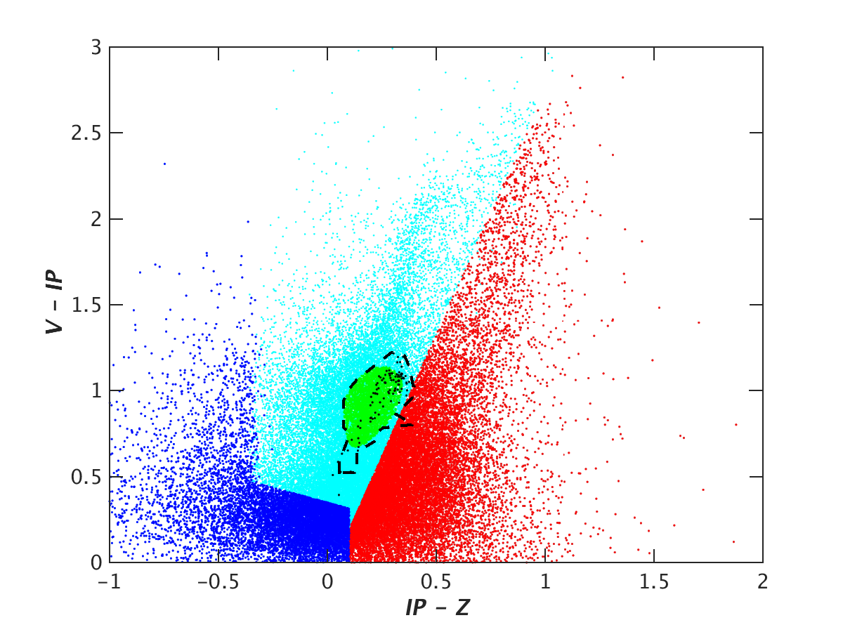
Figure 6.— Showing the selection of background galaxies for the WL analysis, using Subaru $V,i^{\prime}$, and $z^{\prime}$ color-color selection. ”Blue” galaxies are lower left and ”red” galaxies are lower right. Rejected galaxies are shown as cyan. Black dots represent spectroscopically measured cluster members. Galaxies at small cluster-centric radius, outlined by dashes and colored green have been excluded from the analysis.

3.4. Weak-lensing Multi-halo Mass Modeling

We perform a two-dimensional shear fitting (Okabe et al. 2011; Watanabe et al. 2011; Umetsu et al. 2012; Medezinski et al. 2013, 2016), by simultaneously modeling the two components of Abell 2465 as a composite of two spherical halos.

To do this, we construct pixelized maps of the two-dimensional reduced-shear $g(\mbox{\boldmath$\theta$})$ (Equation 6) and its error variance $\sigma_{g}(\mbox{\boldmath$\theta$})$ (Equation (8)) on a Cartesian grid of $20\times 24$ independent cells ($N_{\mathrm{cell}}=480$) with $0.75\arcmin$ spacing. Here we have adopted bin averaging, corresponding to $S=1$ in Equation (6). Our multi-halo modeling is restricted to a central region with $15\arcmin\times 18\arcmin$ that contain the NE and SW components. To avoid systematic errors, we have excluded from our analysis innermost cells lying at $|\mbox{\boldmath$\theta$}|<1\arcmin$ from each of the halos (Oguri et al. 2010; Umetsu et al. 2012), where the surface-mass density can be close to or greater than the critical value, to minimize contamination by unlensed cluster member galaxies (Section 3.3) as well as to avoid the inclusion of strongly lensed background galaxies.

We adopt the Navarro–Frenk–White (Navarro, Frenk, & White 1997; NFW, hereafter) model to describe the mass distribution of each cluster component. The NFW density profile provides a good description of the observed mass distribution in the intracluster regime, at least in an ensemble-average sense (e.g., Umetsu et al. 2011a, 2011b, 2014, 2016; Okabe et al. 2013; Niikura et al. 2015; Okabe & Smith 2016). We specify the NFW model using the halo mass $M_{\mathrm{200c}}$, concentration $c_{\mathrm{200c}}=r_{\mathrm{200c}}/r_{-2}$ with $r_{-2}$ the characteristic radius at which the logarithmic density slope is $-2$, and centroid position on the sky.

We adopt an uninformative log-uniform prior in the halo-mass interval, $0.1\leq M_{\mathrm{200c}}/(10^{14}M_{\odot}\,h^{-1})\leq 100$. We set the concentration parameter for each halo using the theoretical concentration–mass relation of Dutton & Maccio (2014), which is calibrated using a Planck cosmology and is in good agreement with recent cluster lensing observations (Umetsu et al. 2016; Okabe & Smith 2016). For the halo centroid, we assume a Gaussian prior centered on each of the BCG position with standard deviation $\sigma=0.5\arcmin$ ($\textsc{fwhm}=1.18\arcmin$). Accordingly, each of the NFW halos is specified by three model parameters, $(M_{\mathrm{200c}},\Delta\mathrm{RA},\Delta\mathrm{Dec})$, where the centroid ($\Delta\mathrm{RA},\Delta\mathrm{Dec}$) is defined relative to the BCG position.

We use the Markov Chain Monte Carlo algorithm with Metropolis–Hastings sampling to constrain the multi-halo lens model from a simultaneous six-component fitting to the reduced-shear field $g(\mbox{\boldmath$\theta$})$. We employ the shear log-likelihood function of Umetsu et al. (2012; Appendix A.2) and Umetsu et al. (2016).

The marginalized posterior distributions for the multi-halo model are shown in Figure 8. The resulting constraints on the halo masses are summarized as follows:

• $M_{\mathrm{200c}}(\mathrm{NE})=(3.1\pm 1.2)\times 10^{14}M_{\odot}$ ($c_{\mathrm{200c}}=4.40\pm 0.17$),

• $M_{\mathrm{200c}}(\mathrm{SW})=(2.5\pm 1.1)\times 10^{14}M_{\odot}$ ($c_{\mathrm{200c}}=4.49\pm 0.20$),

where we employ the robust biweight estimators of Beers et al. (1990) for the central location (mean) and scale (standard deviation) of the marginalized posterior distributions (e.g., Sereno & Umetsu 2011; Umetsu et al. 2014). The resulting weak-lensing mass estimates are noisy with about 40% uncertainty. The mass ratio between the SW and NE halos is constrained as $M_{\mathrm{200c}}(\mathrm{SW})/M_{\mathrm{200c}}(\mathrm{NE})=0.82\pm 0.51$. At the virial overdensity, we find

• $M_{\mathrm{vir}}(\mathrm{NE})=(3.7\pm 1.5)\times 10^{14}M_{\odot}$ ($c_{\mathrm{vir}}=5.46\pm 0.21$),

• $M_{\mathrm{vir}}(\mathrm{SW})=(2.9\pm 1.3)\times 10^{14}M_{\odot}$ ($c_{\mathrm{vir}}=5.57\pm 0.24$),

These can be compared with the virial masses found in Paper I which are $(4.1\pm 0.8)\times 10^{14}M_{\odot}$ and $(3.8\pm 0.8)\times 10^{14}M_{\odot}$ respectively.

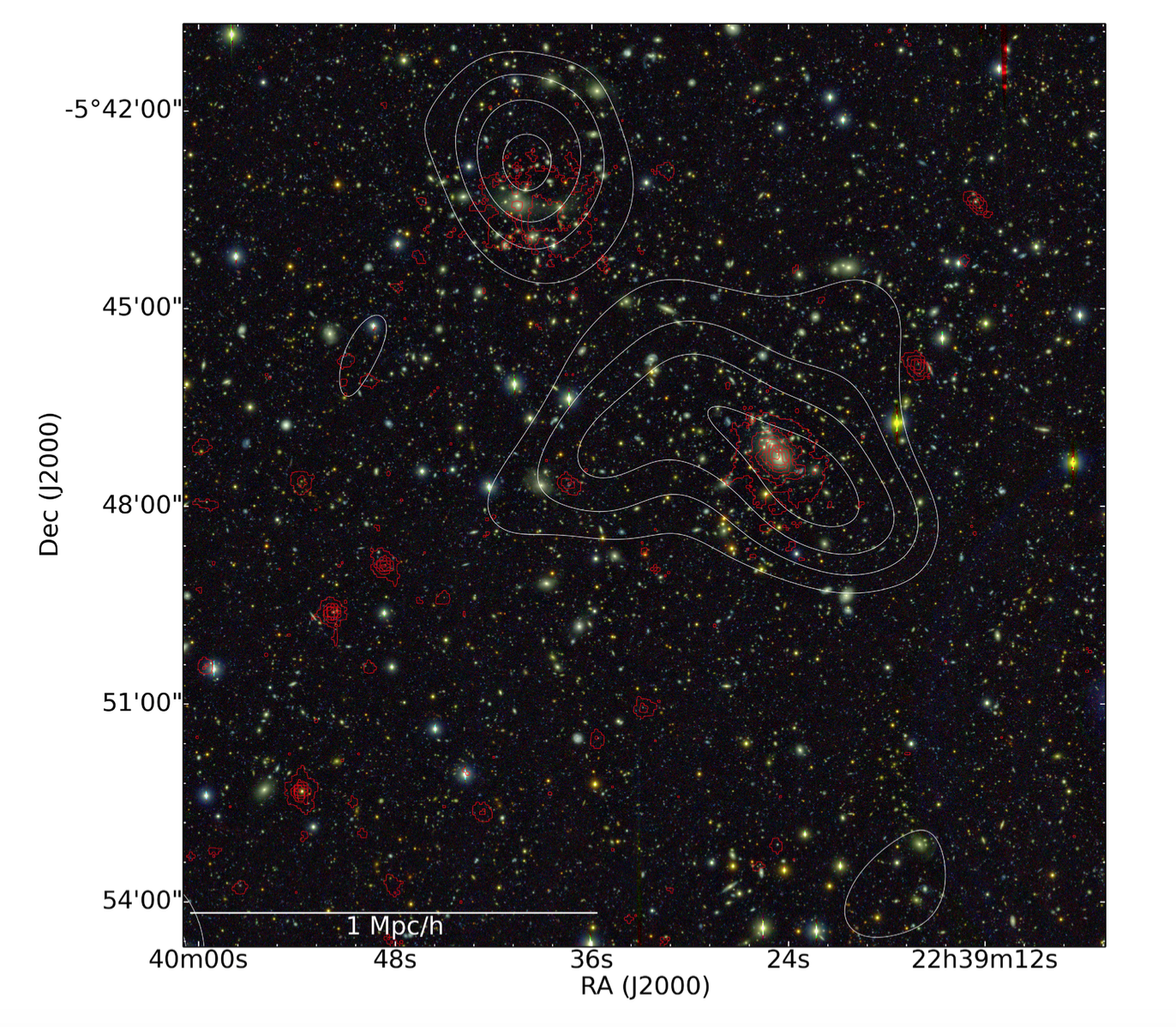
Figure 7.— Subaru $Vi^{\prime}z^{\prime}$ composite color image in the field of Abell 2465, overlaid with weak-lensing mass contours. The mass map is smoothed with a $2\arcmin$ FWHM. The lowest contour is at the $2\sigma$ reconstruction error level ($\kappa=0.034$), and the contour interval is $\Delta\kappa=0.017$. The image is $14\arcmin\times 14\arcmin$ in size. The horizontal bar represents 1 Mpc $h^{-1}$ at the cluster redshift of $z_{\mathrm{l}}=0.245$. The red contours show the smoothed Chandra X-ray brightness data. North is up and east to the left.

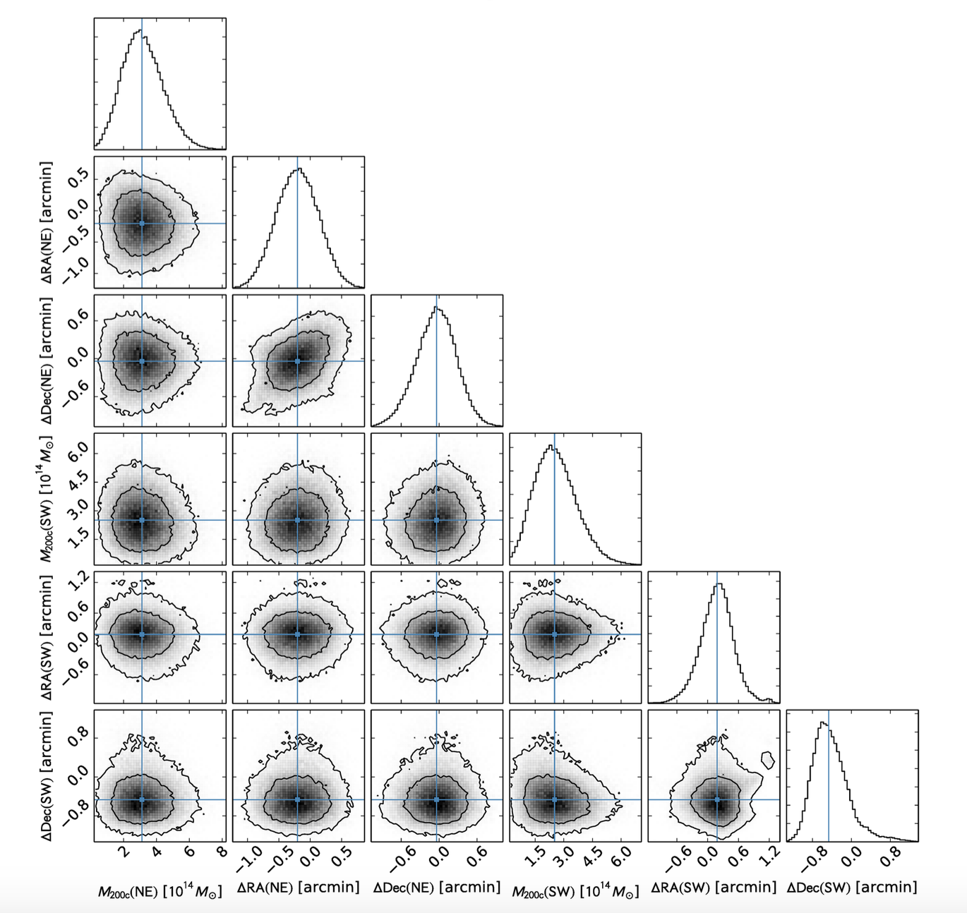
Figure 8.— The posterior distributions of the NFW model parameters for the NE and SW components of Abell 2465, obtained from multi-halo fitting to the two-dimensional Subaru reduced-shear field. For each parameter, the blue solid line shows the biweight central location of the marginalized one-dimensional posterior distribution. For each component, the halo centroid ($\Delta\mathrm{RA}$, $\Delta\mathrm{Dec}$) is measured relative to its brightest galaxy position.

Along the line joining the NE and SW sub-clusters, the offsets of the peaks of the X-ray distributions in Figure 7 are about 0.9 and 0.7 arcmin (or $\sim 0.2$ Mpc) closer together than the weak-lensing peaks. Relative to the BCGs, the weak-lensing offsets are smaller, being about 0.5 arcmin and the distances of the X-ray are about half of this value. Although this is the right order of magnitude for the separation of dark matter and baryonic matter in a cluster merger, given the 1.7 arcmin smoothing, this offset is probably insignificant.

4. The dynamical state of Abell 2465

The radial infall model (Beers, Huchra & Geller 1982) is discussed in Paper I. Two mass points of total mass, $M$, are bound if $V_{r}^{2}R_{\mathrm{p}}\leq 2GM\sin^{2}\phi\cos\phi$. With $V_{r}=205$ km s^-1 (Paper I), Abell 2465 satisfies this condition. Three possible solutions depend on inclination, $\phi$, maximum orbital separation, $R_{\mathrm{m}}$, the system’s age, $t_{0}$, assumed to be the age of the universe at redshift, $z$, and the development parameter, $\eta$. The observed projected distance between the masses centers is $R_{\mathrm{p}}=R\cos\phi$ and the observed velocity difference is $V_{r}=V\sin\phi$.

Using $M=8\pm 1\times 10^{14}M_{\odot}$, $R_{\mathrm{p}}=1.265$ Mpc, and $t_{0}=10.895$ Gyr in Paper I, the three solutions are:

1. $\eta=5.17$ rad, $\phi=5.95\arcdeg$, $R=1.31$ Mpc, $R_{\mathrm{m}}=4.53$ Mpc, $V=-1978$ km s^-1

2. $\eta=3.53$ rad, $\phi=77.5\arcdeg$, $R=6.01$ Mpc, $R_{m}=6.07$ Mpc, $V=-210$ km s^-1

3. $\eta=2.68$ rad, $\phi=81.3\arcdeg$, $R=8.59$ Mpc, $R_{m}=8.81$ Mpc, $V=+208$ km s^-1

Solution (3) has the subclusters moving apart and approaching maximum separation was favored in Paper I, but given the discussion here, that NE and SW have not yet collided, the other two now seem more likely. According to solutions (1) and (2), a core passage would occur in 0.4 or 6.6 Gyr respectively. Possibly the (1) solution is preferable in light of the enhanced star formation induced by the higher impact velocity.

For more detailed modelling, we follow Molnar et al. (2013) who analyzed the Abell 1750 double cluster. This employs the FLASH program which is a parallel Eulerian code originating from the Center for Astrophysical Thermonuclear Flashes at the University of Chicago (Fryxell et al. 2000; Ricker 2008). Further details of the binary merger models are given in Molnar, Hearn, & Stadel (2012). Briefly, the dark matter and galaxies are modelled by truncated NFW profiles and $\beta$-models are used for the gas. The velocities are taken to be isotropic and follow the relations in Lokas & Mamon (2001).

In simulating the Abell 2465 system, we assumed masses, $M_{\mathrm{vir,1}}=4\times 10^{14}M_{\odot}$ and $M_{\mathrm{vir,2}}=3\times 10^{14}M_{\odot}$ and concentration parameters, $c_{\mathrm{vir,1}}=5$ and $c_{\mathrm{vir,2}}=6$, which are consistent with the weak-lensing measurements presented in Section 3.4. We ran FLASH simulations with a range of collisional velocities, $V_{\mathrm{infall}}$ and impact parameters, $P$. We generated mock X-ray observations based on our simulations choosing the phase of the collision which match the observations, and added noise similar to that of the Chandra observations of A2465. The results presented here are relevant to our study of the dynamical state of A2465. Models with $V_{\mathrm{infall}}=1000,2000$, and $3000$ km s^-1 and $P=150$ kpc are shown in Figure 9 (top to bottom). In this figure we show cluster X-ray surface brightness distribution (no noise) based on our FLASH simulations, images of mock Chandra observations (noise added), and, for comparison, the X-ray image from our Chandra observation (left to right). It can be seen from the X-ray surface brightness distribution (right panels), that the morphology of the emission changes as a function of infall velocity. The two X-ray peaks associated with the shock/compression heated intracluster gas of the two components are closer to the centers of the colliding clusters for lower infall velocities. Unfortunately the depth of the X-ray observations is insufficiently deep enough to see the detailed morphology of the interaction region.

Solutions (2) and (3) imply that the two clusters appear close to each other only due to a projection effect, they are actually 6 Mpc and 8.59 Mpc apart, and the collision is close to the LOS ($\phi=77.5\arcdeg$ and $\phi=81.3\arcdeg$). In this case no enhanced X-ray emission should be observed between the two cluster centers, just a simple superposition of their equilibrium gas emission.

Solution (1) of our simplified dynamical analysis suggests that the collision is close to the plane of the sky, $\phi=5.95\arcdeg$, and the intracluster gas of the two components are already interacting (in collision), since $R=1.31$ Mpc is less than the sum of the two virial radii. In this case, we should see enhanced X-ray emission from the shock/compression heated intracluster gas between the two cluster centers. In solution (1), the 3D relative velocity between the sub-clusters is $V=-1978$ km s^-1. Our simulations with infall velocities of $V_{\mathrm{infall}}=1000$ km s^-1and 2000 km s^-1bracket this value (note that the infalling cluster speeds up as it falls in, so its infall velocity should be slightly less than $V=-1978$ km s^-1). Note that at this large distance, $R\geq 1.3$ Mpc, the relative velocity of the infalling cluster is insensitive to the expected impact parameter ($P\lower 2.15277pt\hbox{$\;\buildrel<\over{\sim}\;$}300$ kpc), since it is moving in the shallow outer part of the cluster’s gravitational potential.

Consequently we extract data from our mock images based on our FLASH simulations assuming $V_{\mathrm{infall}}=1000$ km s^-1and 2000 km s^-1from the same regions in the sky used for our Chandra analysis (shown in Figure 4, and derive the X-ray profiles along the line between the two X-ray peaks. In Figure 10 we compare the surface brightness profile between the two cluster centers extracted from our Chandra observations (stars with error bars connected with black thick solid line), and the profiles extracted from our mock observations based on simulations with $V_{\mathrm{infall}}=1000$ km s^-1and 2000 km s^-1(red squares and green diamonds with error bars connected with solid lines of the same color; same data were used in Figure 9). Triangles with error bars connected with a blue solid line represent an X-ray profile assuming no interaction between the two clusters (corresponding to solutions (2) and (3)). As it can be seen from this figure, the simulations predict an enhancement between the two X-ray peaks if there is a collision in progress. The enhancement in the X-ray emission seems to be significant between the two cluster centers even with the low exposure time assumed for the image simulations (the red squares and green diamonds in the middle region are about $1\sigma$ higher than the blue triangles, which represent on-interacting clusters). However, we can see no significant difference between simulations assuming $V_{\mathrm{infall}}=1000$ km s^-1and 2000 km s^-1with the given exposure times. Thus our simulations suggest that A2465 is in a process of collision, the intracluster gas of the two components are already interacting, but we cannot constrain the infall velocity of the system using only our FLASH simulations.

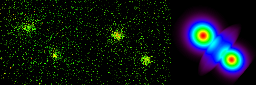
V_infall = 1000 km s^-1

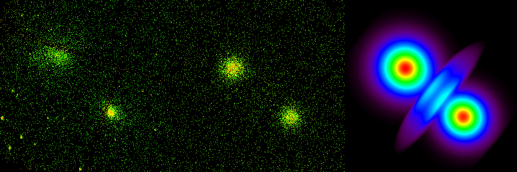
V_infall = 2000 km s^-1

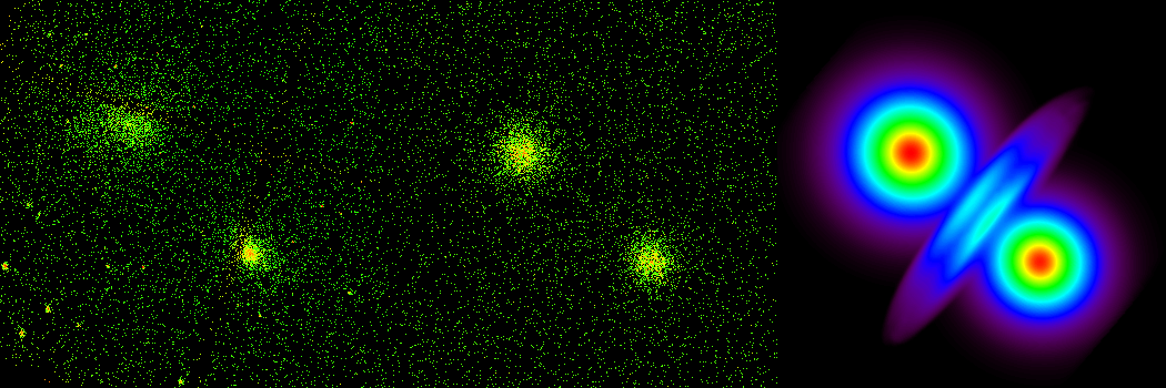
V_infall = 3000 km s^-1

Figure 9.— Examples of simulated X-ray observations based on our FLASH simulations with different infall velocities as marked (V_infall; top to bottom) for Abell 2465 compared with Chandra observations. from right to left: image from Chandra observations; mock X-ray observation fitted to the Chandra flux; model X-ray surface brightness.

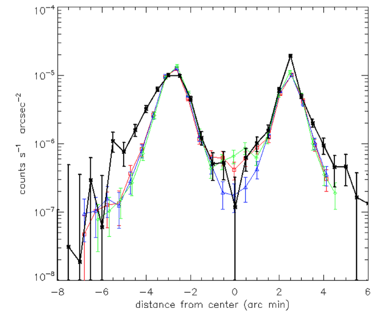
Figure 10.— X-ray surface brightness profiles along the line connecting the two X-ray peaks from Chandra observations (stars with error bars connected with thick black solid lines), from mock observations with V_infall = 1000 and 2000 km s^-1(red squares and green diamonds with error bars connected with solid lines of the same color; presented in Figure 9), and from mock observations assuming that the clusters are not interacting, they look close to each other only in projection (blue triangles with error bars).

5. Discussion

From the increasing number of examples of double and multiple merging galaxy clusters, discovered and analyzed in recent years, these objects can provide information on galaxy formation and evolution, give clues on the interactions of the clusters’ baryonic and dark matter interactions, as well as the behavior of gravitation on Mpc scales. The interactions of different types of dark matter through pressure effects (Ota & Yoshida 2016), dynamical friction and self interacting dark matter (Irshad et al. 2014; Kahlhoefer et al. 2014) or modified gravity (e.g. Del Popolo 2013; Matsakos & Diaferio 2016) could in principle produce observable effects. To date, this has proven difficult due to the complexity of the interacting systems which range from pre-mergers, given in the Introduction (Okabe & Umetsu 2008; Andrade-Santos et al. 2015) as well as the A3407+A3408 pair (Nascimento et al. 2016) to post-core passage objects. However, in many cases the structure geometry is complex. The $\sim 2\times 10^{15}M_{\odot}$ ’El Gordo’ cluster (Jee et al. 2016) only shows one X-ray peak, CIZA J2242.8+5301 is highly elongated (Jee et al. 2015), and CIZA J0107.7+5408 (Randall et al. 2016) is a complex dissociative merger.

Using the basic properties of the two sub-components in Abell 2465 derived above and in Papers I and II, scaling relations for galaxy clusters, the merger indicate no observable effects other than the enhanced star formation found in Paper II. Both clumps follow the cluster $M_{\mathrm{200c}}$–$L_{X}$ relations (e.g. Reiprich & Böhringer 2002; Rykoff et al. 2008) and the $T_{X}$–$M_{\mathrm{200c}}$ relations (e.g. Popesso et al. 2005). However, the SW subcluster appears to have a lower than normal gas fraction, $f_{\mathrm{gas}}=M_{\mathrm{gas}}/M_{\mathrm{hyd}}$. From Table 2, $f_{\mathrm{gas}}=0.10$ for the NE clump, and it is 0.04 for the SW clump. In the $f_{\mathrm{gas}}$–$T_{X}$ relations in Sanderson et al. (2003), Vikhlinin et al. (2006), Sun et al. (2009), Sun (2012), and Lovisari et al. (2015), the corresponding gas fractions are about 0.10.

The reduced entropy, $K/K_{\mathrm{500c}}\approx 0.07,$ for the SW component is in the range for cool-core or gravitationally collapsed clusters (e.g. Pratt et al. 2010) and the higher value ($K/K_{\mathrm{500c}}\approx 0.14$) for the NE could be attributed to a morphologically disturbed cluster due to a separate earlier merging event rather than interaction with the SW. Due to our limited data, this should only be considered indicative rather than conclusive.

The low exposure time of our X-ray observations of A2465 does not allow us to carry out a quantitative dynamical analysis based on $N$-body/hydrodynamical simulations. The infall velocity, impact parameter, etc. of the system can not be derived, but combining a simplified dynamical analysis with FLASH simulation allows us to find an approximate dynamical state of the system, specifically, to distinguish between a non-interacting system and one in an early state of merging. Our FLASH simulations suggest enhanced X-ray emission between the two cluster centers (relative to assuming a simple superposition of the two equilibrium cluster emission), which can be attributed to shock/compression heated intracluster gas due to merging. We have found only one solution, applying our simplified dynamical analysis, which results in a stage of merging, close to solution (1) of the radial infall model with a 3D relative velocity of $V=-1978$ km s^-1 between the clusters and a 3D distance of $R=1.31$ Mpc. Our FLASH simulations cannot constrain the relative velocity (or the infall velocity) alone, but they indicate a pre-core passage state for the cluster.

From these data it appears that the NE and SW components of Abell 2465 resemble the nearer and somewhat less massive double cluster Abell 3716 (PLCKG345.40-39.34) studied by Andrade-Santos et al. (2015), who conclude that that cluster is in a pre-collisional state, and the binary clusters Abell 1750 and 1758 (Okabe & Umetsu 2008) which also appear to be in the early merger stages. Consequently Abell 2465 is an excellent candidate for studying the early stages of galaxy cluster collisions.

The physical separation of the galaxy, gas, and dark matter components is of considerable current interest and has been modelled by many investigators (e.g. Schaller et al. 2015; Massey et al. 2015; Kim, Peter & Wittman 2016). For Abell 2465 this offset is small and appears to be below the reliability of our data so we can only place upper limits. The small 0.2 Mpc weak-lensing to X-ray offset in Section 3.4, however would be comparable to that found in some other clusters, except in the pre-merger state, one expects the gas to trail the galaxies and dark matter. Simulations of merging halos, (e.g. by Vijayaraghavan & Ricker 2015) of merging halos show the stripped gas trails and galaxy wakes which would follow rather than precede the sub-clusters.

It is interesting to note that although the weak-lensing and optical data assign the higher mass to the NE sub-component, from weak lensing it has a more symmetrical profile of mass contours. The SW sub-component with the more compact central region has more unsymetrical and extended outer mass contours that show a flattened shape perpendicular to the line joining the two clumps. This might be a sign of the merging of the two components. Since the subclusters are separated by about 1.2 Mpc, there should be substantial overlap of their halos and therefore the possibility for interaction between the two components. In their current configuration, the components of Abell 2465 appear to show no marked distortions or offsets.

6. Conclusions

The goal of this investigation was to determine the dynamical state of the components of the double galaxy cluster Abell 2465. In advanced mergers these are known to separate. The X-ray data reveal the distribution of the baryonic gas component and the weak lensing shows the distribution of the total mass including dark matter. This can be compared with the distributions of the luminous matter from given in Papers I and II. From this study we draw the following conclusions.

(1) Using the Chandra X-ray observations in Section 2, the X-ray surface profiles of the NE and SW components were fit employing modified $\beta$-models. The NE sub-cluster has a broader profile than the SW component. The Chandra X-ray data provided temperatures, gas and total masses, and gas fractions, and determined a central entropy. This indicates that the NE and SW subclusters have gas masses 1.90 and $0.96\times 10^{13}M_{\odot}$ and total masses 1.85 and $2.17\times 10^{14}M_{\odot}$.

(2) The entropy profiles from the X-ray data differ for the two subclumps. The NE central entropy is higher compared to the SW. This could be due to NE having undergone a recent merger. This seems consistent with NE having the three BCGs which should merge in a short time and SW being more relaxed as it has a sharper central profile and suggestive of a cool core.

(3) Section 2.5 shows that there are no large amounts of X-ray gas between the two sub-clusters of Abell 2465, such as are found in colliding clusters e.g. the Bullet Cluster.

(4) The weak-lensing analysis in Section 3 utilizes Subaru Suprime-Cam $Vi^{\prime}z^{\prime}$ images for the background selection and shape measurements. A two-dimensional shear fitting with simultaneous modeling of the two components of Abell 2465 was conducted. This confirms the corresponding weak-lensing virial masses are 3.7 and $2.9\times 10^{14}M_{\odot}$ and from redshift data are 4 and $3\times 10^{14}M_{\odot}$ (Paper I). The projected mass contours are given in Figure 7 which shows some distortion of the contours but only small offsets between them and the X-ray gas.

(5) From the optical redshift measurements in Paper I, the two sub-clusters of Abell 2465 should be gravitationally bound. The cluster as a whole is of an intermediate mass ($M\lower 2.15277pt\hbox{$\;\buildrel<\over{\sim}\;$}10^{15}M_{\odot}$). The absence of strong X-ray emission between the two sub-components and no large offsets between the galaxies and weak lensing centers, suggest that the two subclusters have not yet collided (i.e pre-core passage). Using the FLASH simulations and radial infall model indicates that they will meet in $\sim 0.4$ Gyr.

It seems clear that the NE and SW components of Abell 2465 are in a pre-merger state. Although there is no large separation of the collisionless and baryonic components, such a system might provide constraints on their interactions as they begin to merge. Future observations that could better determine the orbital parameters would be useful for detailed dynamical modeling.

References

- (1) Abell, G. O. 1958, ApJS, 3, 211
- (2) Ahn, C. P. et al. 2012, ApJS, 2013, 21
- (3) Andrade-Santos, F., Jones, C., Forman, W. R. et al. 2015, ApJ, 803, 108
- (4) Bartelmann, M., Schneider, P. 2001, PhR, 340, 291
- (5) Beers, T. C., Geller, M. J., & Huchra, J. P. 1982, ApJ, 257, 23
- (6) Beers, T. C., Flynn, K., & Gebhardt, K. 1990, AJ, 100, 32
- (7) Belsole, E. et al. 2004, A&A, 415, 821
- (8) Bradač, M. et al. 2008a, ApJ, 681, 187
- (9) Bradač, M. et al. 2008b, ApJ, 687, 959
- (10) Capak, P. et al. 2007, ApJS, 172, 99
- (11) Cavagnolo, K. W., Donahue, M., Voit, G. M., Sun, M. 2009, ApJS, 182, 12
- (12) Clowe, D., Bradač, M., Gonzales, A. H., et al. 2006, ApJ, 648, 109
- (13) Coe, D., Umetsu, K., Zitrin, A., et al. 2012, ApJ, 757, 22
- (14) Cohen, S. A., Hickox, R. C., Wegner, G. A., Einasto, M., Vennik, J. 2014, ApJ, 783, 186
- (15) Condon, J. J., Cotton, E. W., Griesen, E. W., Yin, Q. F., Perley, R. A., Broderick, J. J. 1998, AJ, 115, 1693
- (16) Cavaliere, A. & Fusco-Femiano, R. 1976, A&A, 49, 137
- (17) Dawson, W. A. et al. 2012, ApJ, 747, L42
- (18) Del Popolo A. 2013, AIPC, 1548, 2D
- (19) Dickey, J. M. & Lockman, F. J. 1990, ARA&A, 28, 215
- (20) Dutton, A. A. & Macciò, A. V. 2014, MNRAS, 441, 3359
- (21) Eckert, D., Molendi S., Paltani S. 2011, A&A, 526, 79
- (22) Fryxell, B. et al. 2000, ApJS, 131, 273
- (23) Gonzales, A. H., Sivanandam, S., Zabludoff, A. I., Zaritsky, D. 2013, ApJ, 778, 14
- (24) Helfand, D. I., White, R. L., & Becker, R. H. 2015, ApJ, 801, 26
- (25) Hwang, H. S. & Lee, M. G. 2009, MNRAS, 397, 2111
- (26) Irshad M., Liesenborgs J., Saha P., Williams L. L. R. 2014, MNRAS, 439, 2651
- (27) Jee, M. J. et al. 2014, ApJ, 785, 20
- (28) Jee, M. J. et al. 2015, ApJ, 802, 46
- (29) Ilbert, O. et al. 2009, ApJ, 690, 1236
- (30) Kahlhoefer, F., Schmidt-Hoberg K., Frandsen M. T., Sarkar S. 2014, MNRAS, 437, 2865
- (31) Kitayama, T., Suto, Y. 1996, ApJ, 469, 480
- (32) Lovisari, L., Reiprich, T. H., Schellenberger, G. 2015, A&A, 573, 118
- (33) McDonald, M., Benson, B. A., Vikhlinin, A. 2013, ApJ, 774, 23
- (34) Markevitch, M., Vikhlinin, A. 2007, Physics Reports, 443, 1
- (35) Massey R. et al. 2015, MNRAS, 449, 3393
- (36) Matsakos T., Diaferio A. 2016, arXiv:1603.04943
- (37) Medezinski, E. et al. 2010, MNRAS, 405, 257
- (38) Medezinski, E. et al. 2013, ApJ, 777, 43
- (39) Medezinski, E. et al. 2016, ApJ, 817, 24
- (40) Merten, J. et al. 2011, MNRAS, 417, 333
- (41) Miyazaki, S. et al. 2002, PASJ, 54, 833
- (42) Molnar, S. M., Hearn, S. C., Stadel, J. G. 2012, ApJ, 748, 45
- (43) Molnar, S. M., Chiu, I.-N. T., Broadhurst, T., Stadel, J. G. 2013, ApJ, 779, 63
- (44) Nascimento, R. S., Ribeiro, A. L. B. et al. 2016, MNRAS, 460, 193
- (45) Navarro, J. F., Frenk, C. S., & White, S. D. M. 1997, ApJ, 490, 493
- (46) Niikura, H., Takada, M., Okabe, N., Martino, R., & Takahashi, R. 2015, PASJ, 67, 103
- (47) Nonino, M. et al. 2009, ApJS, 183, 244
- (48) Oguri, M., Takada, M., Okabe, N., & Smith, G. P. 2010, MNRAS, 405, 2215
- (49) Okabe, N., Umetsu K. 2008, PASJ, 60, 345
- (50) Okabe, N., Takada, M., Umetsu, K. et al. 2010, PASJ, 62, 811
- (51) Okabe, N. et al. 2011, ApJ, 741, 116
- (52) Okabe, N., Smith, G. P., Umetsu, K., Takada, M., & Futamase, T. 2013, ApJ, 769, L35
- (53) Okabe, N. & Smith, G.P. 2016, MNRAS, 461, 3794
- (54) Ota, N., Yoshida, H. 2016, PASJ, 68, 19
- (55) Owers, M. S., Randall, S. W., Nulsen, P. E. J., Couch, W. J., David, L. P., Kempner, J. J. 2011, ApJ, 728, 27
- (56) Perlman, E., Horner, D. J., Jones, L. R., Scharf, C. A., Ebeling, H., Wegner, G., Malkan, M. 2002, ApJS, 140, 265
- (57) Pickles, A. J. & Depagne, É. 2010, PASP, 122, 1437
- (58) Poole G. B., Fardal M. A., Babul, A., McCarthy, I. G., Quinn, T., Wadsley, J. 2006, MNRAS, 373, 881
- (59) Popesso 2005, A&A, 433, 431
- (60) Pratt, G. W., Arnaud, M., Piffaretti, R., et al. 2010, A&A, 511, 85
- (61) Randall, S. W. et al. 2016, ApJ, 823, 94
- (62) Reiprich, T., Böhringer, H. 2002, ApJ, 567, 716
- (63) Ricker, P. M. & Sarazin, C. L. 2001, ApJ, 561, 621
- (64) Ricker, P. M. 2008, ApJS, 176, 293
- (65) Roettiger, K., Loken, C., Burns, J. O. 1997, ApJS, 109, 307
- (66) Russell, H. R. et al. ,2012, MNRAS, 423, 236
- (67) Rykoff, E. S. et al. 2008, MNRAS, 387, 28
- (68) Sanderson, A. J. R., Ponman, T. J., Finoguenov, A., Lloyd-Davies, E. J. 2003, MNRAS, 340, 989
- (69) Sereno, M., & Umetsu, K. 2011, MNRAS, 416, 3187
- (70) Sarazin, C. L. 1986, Rev Mod Phys, 58,1
- (71) Schaller, M., Robertson, A., Massey, R., Bower, R. G., Eke, R. G. 2015, MNRAS, 453, L58
- (72) Seigar, M. S., Lynam, P. D., & Chorney, N. E. 2003, MNRAS, 344, 110
- (73) Smith, R. K., Brickhouse, N. S., Liedahl, D. A., Raymond, J. C. 2001, ApJ, 556, L91
- (74) Spergel , Steinhardt P. J. 2000, PhRvL, 84, 3760
- (75) Stacy Y. K., Peter A. H. G., Wittman D. 2016, arXiv:1608630
- (76) Sun M., Voit G. M., Donahue M., Jones C., Forman W., Vikhlinin 2009, ApJ, 693, 1142
- (77) Sun M. 2012, NJPh, 14d5004S
- (78) Takizawa, M. 2000, ApJ, 532, 183
- (79) Umetsu, K. & Broadhurst, T. 2008, ApJ, 684, 177
- (80) Umetsu, K. et al. 2009, ApJ, 694, 1643
- (81) Umetsu, K. et al. 2010, ApJ, 714, 1470
- (82) Umetsu, K. et al. 2011a, ApJ, 729, 127
- (83) Umetsu, K. et al. 2011b, ApJ, 738, 41
- (84) Umetsu, K. et al. 2012, ApJ, 755, 56
- (85) Umetsu, K. et al. 2014, ApJ, 795, 163
- (86) Umetsu, K. et al. 2016, ApJ, 821, 116
- (87) Vijayaragharan, R., Ricker, P. M. 2013, MNRAS, 435, 2713
- (88) Vijayaragharan, R., Ricker, P. M. 2015, MNRAS, 449, 2312
- (89) Vikhlinin, A., McNamara, B. R., Forman, W., Jones, C., Quintana, H., Hornstrup, A. 1998, ApJ, 502, 558
- (90) Vikhlinin, A., Markevitch, M. Murray, S. S., et al. 2005, ApJ, 628, 655
- (91) Vikhlinin, A., Kravtsov, A., Forman, W., Jones, C., Markevitch, M., Murray, S. S., Van Speybroeck, L. 2006, ApJ, 640, 691
- (92) Voit, G. M., Kay, S. T., & Bryan, G. L. 2005, MNRAS, 364, 909
- (93) Wang, Q. D., Owen, F., Ledlow, M. 2004, ApJ, 611, 821
- (94) Watanabe, E., Takizawa, M., Nakazawa, K. et al. 2011, PASJ, 63, 357
- (95) Wegner, G. A. 2011, MNRAS, 413, 1333 (Paper I)
- (96) Wegner, G. A., Chu, D. S., Hwang, H. S. 2015, MNRAS, 447, 1126 (Paper II)
- (97) Zel’dovich, Ya. A. & Raizer Yu. P. 1967, Physics of shock waves and high-temperature hydrodynamic phenomena, New York: Academic Press, ed. Hayes, W. D., Probstein, R. F.
- (98) Zhang, Y.-Y. et al. 2011, A&A, 526, 105