Open quantum generalisation of Hopfield neural networks

Abstract

We propose a new framework to understand how quantum effects may impact on the dynamics of neural networks. We implement the dynamics of neural networks in terms of Markovian open quantum systems, which allows us to treat thermal and quantum coherent effects on the same footing. In particular, we propose an open quantum generalisation of the Hopfield neural network, the simplest toy model of associative memory. We determine its phase diagram and show that quantum fluctuations give rise to a qualitatively new non-equilibrium phase. This novel phase is characterised by limit cycles corresponding to high-dimensional stationary manifolds that may be regarded as a generalisation of storage patterns to the quantum domain.

I Introduction

Neural networks (NNs) Haykin (2004) - artificial systems inspired by the neural structure of the brain - have become essential tools for solving tasks where more traditional rule-based algorithms fail. Examples are pattern and speech recognition Bishop (2006), artificial intelligence Mnih et al. (2015); Silver et al. (2016), and the analysis of big data Hinton and Salakhutdinov (2006). All these NNs evolve according to the laws of classical physics.

It is widely believed that computational processes can benefit by exploiting the properties of quantum mechanics. Seminal works by Shor Shor (1999) and Grover Grover (1997) have proved the existence of quantum algorithms that systematically outperform their classical counterparts. More recently, there has been a growing interest in proposing and realizing quantum architectures that may be possibly used in the future as quantum computers: for instance, Shor’s algorithm for the factorization of integer numbers has been implemented on a small 11-qubits trapped-ion system Monz et al. (2016) and D-Wave machines, based on superconducting qubits, have shown potential speedup in solving a particular class of NP-hard problems via quantum annealing Denchev et al. (2016). Although the accurate control of large qubit registers (the scalability challenge) is non-trivial and the computational speedup of the latter is still debated Mandrà et al. (2016); Nishimori (2016); Albash et al. (2017), these represent a concrete step towards large-scale quantum information processors.

An important and timely question is whether it is possible to take advantage of quantum effects in NN computing Biamonte et al. (2016). To our knowledge, only a few studies exist on the learning capacity of quantum perceptron models Lewenstein (1994); Wiebe et al. (2016) and on quantum Boltzmann machines Amin et al. (2016). To date, however, none of the existing proposals Ventura and Martinez (2000); Ezhov and Ventura (2000); Gupta and Zia (2001) allows to define a satisfactory framework to consider quantum effects in NN dynamics. The problem is a conceptual one: the dynamics of closed quantum systems is governed by deterministic temporal evolution equations, whereas NNs are always described by dissipative dynamical equations, thus preventing any straightforward generalization of NNs computing in quantum systems Schuld et al. (2014). Here we overcome this obstacle, by proposing a framework for quantum NNs based on open quantum systems (OQSs). We consider, in particular, the conceptually simplest case of Markovian dynamics, where the evolution of the density matrix is described by a Lindblad equation Breuer and Petruccione (2002).

In order to make our ideas concrete we introduce a generalisation based on OQSs of one of the most studied NN systems, the Hopfield model Hopfield (1982) (see Fig. 1). The dissipative part of the dynamics corresponds to the thermal stochastic dynamics of the classical model (often realised via classical Monte Carlo dynamics), while quantum effects are due to a transverse field Hamiltonian that turns this classical equilibrium system into a quantum non-equilibrium one. In this approach, the result of a NN computation is imprinted on the long time density matrix, whose properties as a function of the control parameters (temperature, quantum driving, initial state) determine the phase diagram of the system. This setup reduces to the classical Hopfield NN when the quantum Hamiltonian is removed. By means of mean-field methods (which are exact for fully connected models such as this one) we calculate the phase diagram of the model, and show that a new non-equilibrium phase, characterized by the presence of limit cycles (LCs), arises due to the competition between coherent and dissipative dynamics. This may be regarded as a quantum generalisation of the retrieval phase of the classical Hopfield model.

Originally, the Hopfield NN was introduced as a toy model of associative memory. In the human brain memory patterns are supposed to be retrieved by association. In a NN, this translates in the following: when a pattern similar enough to one of those stored is presented to the NN, the system is able to retrieve the correct one via classical annealing. The two fundamental ingredients to reproduce this are: (i) a dynamics on a system of $N$ binary spins ($\sigma_{i}=\pm 1$, $i=1,\dots,N$), that represent neuron activity ($+1$ firing and $-1$ silent); (ii) an appropriate prescription for the couplings $J_{ij}$ that connect the $i$-th neuron with the $j$-th one, which must be able to store a set of $p$ different memory patterns $\xi_{i}^{(\mu)}$ (i.e. fixed spin configurations) with $i=1,\dots,N$, $\mu=1,\dots,p$ . In this language, memory retrieval denotes a phase in which the dynamics drives the system towards configurations which are closely resembling one of the $\xi_{i}^{(\mu)}$ for some $\mu$. It turns out that the following discrete time asynchronous dynamics fulfills these requirements:

$$\sigma_{i}(t+1)=\text{sign}\left(\sum_{j\neq i}J_{ij}\sigma_{j}(t)\right)\,,\quad J_{ij}=\frac{1}{N}\sum_{\mu=1}^{p}\xi_{i}^{(\mu)}\xi_{j}^{(\mu)}\,.$$ (1)

Indeed Eq. (1) describes a zero temperature Monte Carlo dynamics (that can be easily generalized to include thermal effects (Amit et al., 1985a)). Moreover it can be proven that this dynamics minimizes the energy function $E=-\frac{1}{2}\sum_{i\neq j}J_{ij}\sigma_{i}\sigma_{j}$, namely an Ising model with pattern-dependent couplings and the global minima of $E$ are precisely the memory patterns $\xi_{i}^{(\mu)}$ (as long as $p\ll N$). Techniques used in the statistical physics of disordered systems enable to investigate Hopfield NNs (and more general types of NNs) quantitatively Amit et al. (1985a, b, 1987). In statistical physics language, the retrieval phase is the low temperature phase corresponding to an energy landscape where memory patterns are stable states of the NN, i.e. the thermal equilibrium stationary states; see Fig. 1.

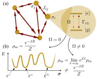
Figure 1: Sketch of the classical-to-quantum mapping for the Hopfield NN. (a) In the Hopfield model neurons (dots) are binary spins describing the activity of the neurons (+1 firing, -1 silent). The OQSs framework allows us to study the competition between thermal and quantum effects. In particular, the $i$-th neuron changes its activity state at a rate $\Gamma_{i\pm}$ as in the classical model or undergoes a quantum state change, due to the coherent driving introduced in Eq. (4). (b) If $\Omega=0$, the stationary state is at thermal equilibrium. The qualitative behavior of the energy function of the classical NN is sketched in a one dimensional projection of the configurational space. Memory patterns are stored as the energy minima of the energy function. Whenever the NN is initialized close enough (close in the sense of the Hamming distance between spin configurations) to a specific memory pattern, the dynamics in Eq. (1) allows to retrieve the corresponding stored pattern. In the presence of quantum effects ($\Omega\neq 0$), the nature of the stationary state can be non-trivial, i.e. it may be non-thermal, due to the competition between quantum coherence and irreversible classical dynamics.

II Methods

II.1 Open quantum Hopfield NNs

To introduce quantum effects, we employ a description of the NN dynamics in terms of open quantum master equations. The starting point of our analysis is a master equation in Lindblad form for the density matrix $\rho$:

$$\dot{\rho}=-i[H,\rho]+\sum_{i=1}^{N}\sum_{\tau=\pm}\left(L_{i\tau}^{\phantom{\dagger}}\rho L_{i\tau}^{\dagger}-\frac{1}{2}\{L_{i\tau}^{\dagger}L_{i\tau}^{\phantom{\dagger}},\rho\}\right)\,,$$ (2)

where we define a set of jump operators as follows:

$$L_{i\pm}=\Gamma_{i\pm}\sigma_{i}^{\pm},\quad\Gamma_{i\pm}=\frac{e^{\mp\beta/2\Delta E_{i}}}{(2\cosh(\beta\Delta E_{i}))^{\frac{1}{2}}}\,.$$ (3)

Here $\beta=1/T$ is the inverse temperature, $\Delta E_{i}=\sum_{j\neq i}J_{ij}\sigma_{j}^{z}$ the change in energy under flipping of the $i$-th spin, and $\sigma_{i}^{\pm}=(\sigma_{i}^{x}\pm i\sigma_{i}^{y})/2$, with $\sigma^{x,y,z}$ the Pauli matrices. Quantum effects are included by a uniform transverse field in the $x$-direction, corresponding to a Hamiltonian,

$$H=\Omega\sum_{i=1}^{N}\sigma_{i}^{x}\,.$$ (4)

In the absence of this term, Eq. (2) describes a classical stochastic dynamics: any initial density matrix that is diagonal in the $\sigma^{z}$ basis remains diagonal under the evolution and Eq. (2) reduces to $\dot{P}=\sum_{i=1}^{N}\sum_{\tau=\pm}\Gamma_{i\tau}^{2}\left[\sigma_{i}^{\tau}-\frac{1}{2}\left(1+\tau\sigma_{i}^{z}\right)\right]P$, where $P$ is the probability vector formed by the diagonal of $\rho$. The rates $\Gamma_{i\tau}^{2}$ obey detailed balance with respect to the Boltzmann distribution for energy $E$ at temperature $T$, so that this is the master equation for the classical Hopfield NN, as shown in the supplementary material (SM) see supplemental material .

II.2 Derivation of the mean field equations

Starting from Eq. (2), the corresponding equation for the evolution of an observable $O$ is given by:

$$\begin{split}\dot{O}&=i[H,O]+\sum_{k}L^{\dagger}_{k}OL_{k}-\frac{1}{2}\{L^{\dagger}_{k}L_{k},O\}\,,\end{split}$$ (5)

where $H$ is given in Eq. (4) and the jump operators are those in Eq. (3). Here we are interested in the evolution of the local observables $\sigma^{\alpha}_{i}$ ($\alpha=x,y,z$). The equation of motion for $\sigma^{z}_{i}$ reads (see SM for more details):

$$\dot{\sigma}^{z}_{i}=2\Omega\sigma^{y}_{i}-\gamma\sigma_{i}^{z}+\gamma\tanh\left(\beta\Delta E_{i}\right),$$ (6)

which in the absence of dissipation ($\gamma=0$) would simply describe Rabi oscillations of frequency $2\Omega$ about the $x$ axis. This clearly shows that the decoupling of the classical subspace does not hold any more: in fact, the equations for $\sigma_{z}^{i}$ do not close and we need to write additional ones for $\sigma_{i}^{x/y}$ or, equivalently, $\sigma_{i}^{\pm}$. These are generically more involved, since these operators do not commute with the $\Gamma$s. To simplify the respective Lindblad equations, we will make use in the following of the anticommutation relations, which in particular imply that

$$f(\sigma_{1}^{z},\cdots,\sigma_{j}^{z},\cdots,\sigma_{N}^{z})\sigma^{\pm}_{j}=\sigma^{\pm}_{j}f(\sigma_{1}^{z},\cdots,-\sigma_{j}^{z},\cdots,\sigma_{N}^{z})\,,$$ (7)

for any function $f$ with a power series representation. Let us consider the equation for $\sigma_{i}^{+}$:

$$\dot{\sigma}_{i}^{+}=-i\Omega\sigma_{i}^{z}+\gamma\sum_{l}\sigma_{l}^{-}\Gamma_{l+}\sigma_{i}^{+}\Gamma_{l+}\sigma_{l}^{+}-\frac{\gamma}{2}\sum_{l}\left(\{\sigma_{l}^{-}\Gamma_{l+}\Gamma_{l+}\sigma_{l}^{+},\sigma_{i}^{+}\}+(+\leftrightarrow-)\right)\,.$$ (8)

Our aim is now to move all the $\Gamma$’s to the right. This is done applying property (7). Introducing the notation

$$\Gamma_{ls}^{(i)}=\Gamma_{ls}(\sigma_{1}^{z},\cdots,-\sigma^{z}_{i},\cdots,\sigma^{z}_{N})\,,$$ (9)

where $s\in\set{+,-}$. Eq. (8) can be written in a compact form as

$$\dot{\sigma}^{+}_{i} =-i\Omega\sigma_{i}^{z}-\frac{\gamma}{2}\sigma_{i}^{+}(\Gamma_{i+}^{2}+\Gamma_{i-}^{2})+\frac{\gamma}{2}\sigma^{+}_{i}\sum_{l\neq i}(1-\sigma_{l}^{z})\left(\Gamma_{l+}^{(i)}\Gamma_{l+}-\frac{1}{2}\Gamma_{l+}^{(i)}\Gamma_{l+}^{(i)}-\frac{1}{2}\Gamma_{l+}\Gamma_{l+}\right)+$$

$$+\frac{\gamma}{2}\sigma^{+}_{i}\sum_{l\neq i}(1+\sigma_{l}^{z})\left(\Gamma_{l-}^{(i)}\Gamma_{l-}-\frac{1}{2}\Gamma_{l-}^{(i)}\Gamma_{l-}^{(i)}-\frac{1}{2}\Gamma_{l-}\Gamma_{l-}\right)\,.$$ (10)

The equation for $\sigma_{i}^{-}$ is simply obtained via hermitian conjugation of the one above. These equations can be simplified recognizing that $\Gamma$ and $\Gamma^{(i)}$ depend on two configurations which differ by a single spin (the $i$-th one). It could be thereby reasonably expected that $\Gamma\approx\Gamma^{(i)}$ up to finite-size corrections which scale as $1/N$ (this is true as long as $p\ll N^{2}$, see also SM for more details). Therefore, we can safely neglect these terms in the thermodynamic limit, which produces a considerably simplified form of the dynamical equations

$$\dot{\sigma}_{i}^{\pm}=\mp i\Omega\sigma^{z}_{i}-\frac{\gamma}{2}\sigma_{i}^{\pm}.$$ (11)

The equations can be further simplified by expressing them in the $(x,y,z)$ basis:

$$\dot{\sigma}_{i}^{z} =2\Omega\sigma_{i}^{y}-\gamma\sigma_{i}^{z}+\gamma\tanh\left(\beta\Delta E_{i}\right),$$ (12a)

$$\dot{\sigma}_{i}^{y} =-2\Omega\sigma_{i}^{z}-\frac{\gamma}{2}\sigma_{i}^{y},$$ (12b)

$$\dot{\sigma}_{i}^{x} =-\frac{\gamma}{2}\sigma_{i}^{x}.$$ (12c)

Interestingly enough, the equation for $\sigma_{i}^{x}$ decouples from the others and one can conveniently restrict to the $y$ and $z$ components only.

At this stage, we define a suitable set of collective variables as:

$$s_{\mu}^{\alpha}=\frac{1}{N}\sum_{i=1}^{N}\xi_{i}^{(\mu)}\sigma_{i}^{\alpha}\quad\mu=1,\cdots,p\,;\,\,\,\,\,\alpha=x,y,z\,.$$ (13)

These observables can be thought as the overlap between the $\mu$-th memory and the $\alpha$ component of the spins. The equations for these collective variables read

$$\dot{\mathbf{s}}^{z} =2\Omega\mathbf{s}^{y}+\frac{\gamma}{N}\sum_{i=1}^{N}\boldsymbol{\xi}_{i}\tanh(\beta\boldsymbol{\xi}_{i}\cdot\mathbf{s}^{z})-\gamma\mathbf{s}^{z}\,,$$ (14)

$$\dot{\mathbf{s}}^{y} =-2\Omega\mathbf{s}^{z}-\frac{\gamma}{2}\mathbf{s}^{y}\,,$$ (15)

where the vectorial notation now groups the pattern indices, not the positional ones: in other words, these are $p$-uples of operators $\mathbf{s}^{\alpha}=\left(s^{\alpha}_{1},\ldots s^{\alpha}_{p}\right)^{\intercal}$ and numbers $\boldsymbol{\xi}_{i}=\left(\xi^{(1)}_{i},\ldots\xi^{(p)}_{i}\right)^{\intercal}$.

III Results

III.1 Mean-field solution

Since the NN is defined in terms of fully-connected interactions, the mean-field approximation should be exact see supplemental material and amounts to considering the evolution of the averaged collective variables $m_{\mu}^{z,y}=\braket{s_{\mu}^{z,y}}$ neglecting correlations between them see supplemental material . The evolution equations then read:

$$\dot{\mathbf{m}}^{z} =2\Omega\mathbf{m}^{y}+\frac{1}{N}\sum_{i=1}^{N}\boldsymbol{\xi}_{i}\tanh(\beta\boldsymbol{\xi}_{i}\cdot\mathbf{m}^{z})-\mathbf{m}^{z}\,,$$ (16)

$$\dot{\mathbf{m}}^{y} =-2\Omega\mathbf{m}^{z}-\frac{1}{2}\mathbf{m}^{y}\,,$$ (17)

where we introduced a vectorial notation for both the collective variables and the memory patterns, $\dot{\mathbf{m}}^{\alpha}=\left(m_{1}^{\alpha},\ldots,m_{p}^{\alpha}\right)$. $m^{z}_{\mu}$ represents the overlap between the $\mu$-th memory pattern and the neuronal configuration of the system (in the $z$ direction), and thus can be used as an order parameter: if in the stationary state $m_{1}^{z}\approx(1,0,\dots,0)$, this means that the NN correctly retrieved the first pattern stored (and similarly for the other $p-1$ patterns). Setting $\dot{\mathbf{m}}^{z}=\dot{\mathbf{m}}^{y}=\mathbf{0}$ in Eqs. (16,17) we get the equations for the stationary solutions:

$$(1+8\Omega^{2})\mathbf{m}^{z}=\overline{\boldsymbol{\xi}\tanh(\beta\boldsymbol{\xi}\cdot\mathbf{m}^{z})}\,,$$ (18)

where we have assumed self-averaging, typical of disordered systems Mézard et al. (1990) in the large $N$ limit, i.e., $1/N\sum_{i=1}^{N}f(\boldsymbol{\xi}_{i})\rightarrow\overline{f(\boldsymbol{\xi})}$, where $\overline{(\cdot)}$ is the average over the disorder distribution. Equations (16,17) allow to study the interplay between the retrieval and the paramagnetic phases of the NN. It is worth remarking, however, that a more general approach, involving the replica method, is required to deal with the spin glass phase arising when an extensive number of memory patterns is loaded into the NN Amit et al. (1985b). In the following we focus on the retrieval phase of our OQS, which amounts to considering the case of a finite number of patterns $p$.

As a first step, we notice that Eq. (18) has the same form of the mean-field equation obtained for the classical Hopfield NN Amit et al. (1985a): in particular a suitable rescaling of $\mathbf{m}^{z}$ with an effective temperature $T_{\rm eff}=T(1+8\Omega^{2})$ establishes their equivalence. This means that the structure of the stationary points of the dynamics is equivalent to the classical one up to a rescaling of the temperature. In particular, the retrieval solutions $\mathbf{m}^{z}\approx(1,\dots,0)$, the paramagnetic solution $\mathbf{m}^{z}=\mathbf{0}$, as well as the whole set of metastable states (spurious memories) Amit et al. (1985a) are still fixed points of the quantum dynamics. Closer inspection of Eqs. (16,17) reveals, however, that quantum driving does more than just rescale temperature.

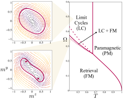
Figure 2: Phase diagram of the OQS generalization of the Hopfield model in the $(T,\Omega)$ plane. The NN displays a paramagnetic phase in the high temperature regime, with a stable attractor in $\mathbf{m}^{z}=\mathbf{0}$. The boundary of the paramagnetic phase is established by looking at the stability of this attractor. In the low $T$ and $\Omega$ regime the system is in the ferromagnetic (retrieval) phase, whereas for low $T$ but sufficiently large $\Omega$, the NN displays a LC (top left), which is the only stable attractor once the ferromagnetic solutions become unstable (above the solid line between FM and LC phases). However the LC appears well below this line (and above the dotted line), producing a small region of phase coexistence (see flux diagram at bottom left). Above the dashed line and for $T<2/3$, the ferromagnetic solutions disappear.

Beyond these stationary solutions, the mean-field equations (16,17) also display time-dependent periodic solutions at long times. A simple way to gain insight on this new feature is to consider a high-$T$ expansion of Eqs. (16,17) up to the first non-linear order. In this case the equations become analogous to a Lotka-Volterra dynamical system, widely studied in the literature on ecological systems Takeuchi (1996). Under appropriate conditions, a Lotka-Volterra system is known to have limit cycles (LCs) solutions.

The observation above suggests that our open quantum Hopfield NN can feature at least three possible phases in the $(T,\Omega)$ plane: (i) a paramagnetic phase where the dynamics converges to the trivial solution $\mathbf{m}^{z}=\mathbf{0}$; (ii) a retrieval phase where the attractor of the system is one of the non-trivial solutions of Eq. (18); (iii) a novel time-dependent stationary phase, emerging from the competition between the dissipative and coherent dynamics.

III.2 Phase diagram

To characterize the phase diagram of this OQS in the $(T,\Omega)$ plane, we follow two different routes: (i) we solve numerically the mean-field equations at low $p$ by averaging over disorder using the factorized probability distribution $P(\boldsymbol{\xi})=\prod_{\alpha=1}^{p}p(\xi^{(\alpha)})$ with $p(\xi)=1/2\delta(\xi-1)+1/2\delta(\xi+1)$; (ii) we perform a Lyapunov linear stability analysis Lyapunov (1992), namely we study the dynamical stability of the stationary points under small perturbations (see see supplemental material for details). Through either approach we identify the boundaries of the different phases. The numerical solution of the mean field equations (16), (17) is obtained with a standard numerical integrator available in Wolfram Mathematica.

The phase diagram of the NN is summarized in Fig. 2. For $T>2/3$ and $\Omega>\sqrt{(1-T)/8T}$ the system is in the paramagnetic phase. Retrieval is possible in the low temperature and low $\Omega$ regime, whereas the dynamics features LCs as a stationary manifold in the low temperature and high coherence regime. At the boundary between the retrieval and the LC phase, we recognize a small region where the two phases coexist: initializing the system close enough to $(\mathbf{m}^{z},\mathbf{m}^{y})=(\mathbf{0},\mathbf{0})$, drives the NN towards the retrieval solutions, whereas initial conditions chosen outside a critical hypervolume centered around $(\mathbf{0},\mathbf{0})$ converge to the LC (see insets in Fig 2).

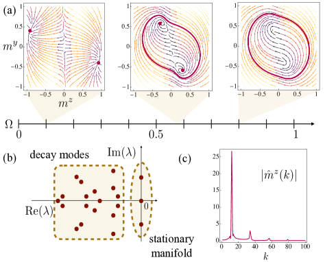
Figure 3: Qualitative spectrum of the superoperator in the LC phase. (a) From left to right flux diagrams of the mean-field dynamics at $T=0.15$, $\Omega=0.1\,,0.58\,,0.8$. The different attractors are highlighted in each panel. In the bulk of the LC phase the maximum overlap with one of the stored patterns is $\sim 0.8$, independently from the initial conditions, suggesting that also this phase can be interpreted as a retrieval phase. (b) Sketch of the spectrum of a plausible Liovillian super-operator describing the LC shown in (a). Time-dependent periodic stationary states require at least a conjugate pair of purely imaginary eigenvalues. (c) The structure of the Fourier components $|\hat{m}^{z}(k)|$ of the top right LC, justifies the single frequency approximation made in the main text.

For a single pattern, $p=1$, we are able to rigorously prove the presence of a LC phase, since Eqs. (16) and (17) can be recast in Liénard form Palit and prasad Datta (2010), (see also see supplemental material ) for $T<2/3$ and $T>(8\Omega^{2}+1)^{-1}$. The Liénard theorem Hirsch et al. (2003) guarantees the existence, uniqueness and stability of a LC (which wraps around the origin).

The LC phase can be interpreted as a new quantum retrieval phase: for low enough temperatures, in fact, independently from the initial conditions the NN is always driven towards a LC with a large oscillation amplitude. For instance, the case reported in Fig. 3a (corresponding to $T=0.15$) shows oscillations reaching a maximum overlap of $\sim 0.8$ with the single stored pattern. Limit cycles of this kind (involving mostly a single overlap) also exist for generic $p>1$. For $p\leq 4$ we have performed a systematic numerical study in the LC phase in the range of parameters $0.4\leq T\leq 0.66$ and $0.4\leq\Omega\leq 1$ (using the same distribution of the couplings mentioned above) finding that at long times oscillations involve at most two overlaps, while all the remaining $p-2$ asymptotically vanish. More importantly, starting from an initial condition with large overlap with one of the patterns (say, the $\mu$-th one) and significantly smaller overlap with the remaining ones seems to always lead to oscillations in the $(m^{z}_{\mu},m^{y}_{\mu})$ plane and vanishing ones in the others. These findings are also supported by preliminary investigations for $p<10$ and seem plausible for general $p$ by looking at the theoretical argument presented in section 3C of the SM. This is somewhat reminiscent of the retrieval phase, where the dynamics proceeds towards the pattern it initially had larger overlap with. Furthermore, when cooling the system at large $\Omega$, LC attractors emerge before the appearance of the stable fixed points, which hints at the possibility of a correspondence between fixed point attractors $\xi_{i}^{(\mu)}$ and LC ones. At this level, this aspect comes out as a numerical finding and will require future work in order to be explored and established in more detail. It is moreover noteworthy that the fundamental properties of the Hopfield dynamics are rather robust against the introduction of a coherent term such as the transverse field we use in this work. It is worth remarking that this robustness is closely related to symmetry arguments: indeed the generalized $\mathrm{Z}_{2}$ symmetry broken in the FM phase of the classical model is still broken in the LC phase. Here, additionally, the stationary state spontaneously breaks the time translation symmetry, which should correspond to the appearance of a Goldstone mode, as found in Chan et al. (2015).

IV Discussion

Examples of LC phases in classical Hopfield NNs with asymmetric couplings exist Coolen and Ruijgrok (1988); Evans (1989); ichi Inoue (2011). However, the LC phase that we find here is intimately related to the competition between coherent and dissipative dynamics. The persistence of oscillations in the long time limit implies the survival – to a degree – of quantum coherence. To substantiate this claim, we argue in the following what the structure of the stationary manifold of the Lindblad equation should be, following the classification of Refs. Baumgartner and Narnhofer (2008); Albert and Jiang (2014); Albert et al. (2016) for the case of systems with finite-dimensional Hilbert spaces.

By formally integrating Eq. (2) we get $\rho(t)=e^{t\mathcal{L}}\rho_{\mathrm{in}}$, where $\mathcal{L}$ is the generator of the open quantum dynamics [i.e., $\mathcal{L}\rho$ is shorthand for the r.h.s. of Eq. (2)], and $\rho_{\mathrm{in}}$ is the initial state. Assuming $\mathcal{L}$ to be diagonalizable, the density matrix can be further expanded as Macieszczak et al. (2016):

$$\rho(t)=\sum_{l=1}^{2^{2N}}c_{l}e^{t\lambda_{l}}R_{l}\,,$$ (19)

where $\lambda_{l}$ are the eigenvalues, $R_{l}$ are the right eigenmatrices of $\mathcal{L}$, i.e. $\mathcal{L}R_{l}=\lambda_{l}R_{l}$, and $c_{l}$ the components of the initial state on these eigenmodes. Because of preservation of probability and positivity, the eigenvalues of $\mathcal{L}$ have non-positive real parts and are either real or come in complex conjugate pairs. The stationary manifold is constructed from all the $R_{l}$ for which $\mathrm{Re}(\lambda_{l})=0$; we define $n$ its dimension and reorder the eigenvalues such that the zero ones appear first. If $\lambda_{l}=0\ \forall\ l=1,\ldots,n$ then each initial state maps to a state in the stationary manifold asymptotically and no time dependence survives at long times. To allow for limit cycles, $\mathcal{L}$ must display at least a pair of conjugate, purely-imaginary eigenvalues $\pm i\omega$, as sketched in Fig. 3b. The long time evolution due to the presence of these eigenvalues is unitary and one could formally define a corresponding reduced Hamiltonian acting coherently on the stationary subspace Zanardi and Campos Venuti (2014); Albert et al. (2016); Macieszczak et al. (2016).

A Fourier analysis deep in the LC phase (see Fig 3c) justifies a single frequency approximation for the stationary state, leading to $\rho_{\mathrm{ss}}(t)\sim R_{0}+R_{1}+R_{2}e^{i\omega t}+R_{2}^{\dagger}e^{-i\omega t}$, that allows to obtain a quantitative agreement with the numerics by requiring that the $R_{i}$’s are such that: $\operatorname{Tr}\left(s^{\alpha}R_{0/1}\right)=0$, $\operatorname{Tr}\left(s^{z}R_{2}\right)=\bar{m}^{z}$ and $\operatorname{Tr}\left(s^{y}R_{2}\right)=\bar{m}^{y}e^{i\epsilon}$. This choice reproduces a LC in the $(m^{z},m^{y})$ plane parameterized as $m^{z}(t)=\operatorname{Tr}\left(s^{z}\rho_{\mathrm{ss}}(t)\right)\sim\bar{m}^{z}\cos(\omega t)$ and $m^{y}(t)=\operatorname{Tr}\left(s^{y}\rho_{\mathrm{ss}}(t)\right)\sim\bar{m}^{y}\cos(\omega t+\epsilon)$ (with $\epsilon$ a proper real phase).

V Conclusions

We proposed a framework based on open quantum systems to investigate quantum effects in the dynamics of neural networks. It is worth remarking that our implementation is conceptually different from recent results where Hopfield-like unitary evoultions have been found in the context of multimodal cavity quantum electrodynamics with disorder Gopalakrishnan et al. (2011); Strack and Sachdev (2011); Rotondo et al. (2015). We applied this approach to an open system quantum generalization of the simplest model of associative memory, the Hopfield model. As in the classical case it is possible to use a mean-field treatment to determine the phase diagram. We identified a retrieval phase with fixed points associated to classical patterns and quantum effects can be accounted for by an effective temperature. We moreover found a novel phase characterized by limit cycles which are a consequence of the quantum driving. Our approach is a natural extension of the NN paradigm into the domain of open quantum systems. It shows that the resulting phase structure of such systems can indeed be richer than that of their classical counterparts. Future investigations are needed in order to clarify whether practical applications of NNs can benefit from quantum effects. For instance, a relevant question is whether the LC phase discovered here has some interpretation from the statistical learning theory viewpoint.

VI Acknowledgments

The research leading to these results has received funding from the European Research Council under the European Union’s Seventh Framework Programme (FP/2007-2013) / ERC Grant Agreement No. 335266 (ESCQUMA), the H2020-FETPROACT-2014 Grant No.640378 (RYSQ), and EPSRC Grant No. EP/M014266/1. P.R. acknowledges funding by the European Union through the H2020 - MCIF No. 766442.

References

- Haykin (2004) S. Haykin, Neural Networks 2 (2004).
- Bishop (2006) C. M. Bishop, Machine Learning 128 (2006).
- Mnih et al. (2015) V. Mnih, K. Kavukcuoglu, D. Silver, A. A. Rusu, J. Veness, M. G. Bellemare, A. Graves, M. Riedmiller, A. K. Fidjeland, G. Ostrovski, et al., Nature 518, 529 (2015).
- Silver et al. (2016) D. Silver, A. Huang, C. J. Maddison, A. Guez, L. Sifre, G. Van Den Driessche, J. Schrittwieser, I. Antonoglou, V. Panneershelvam, M. Lanctot, et al., Nature 529, 484 (2016).
- Hinton and Salakhutdinov (2006) G. E. Hinton and R. R. Salakhutdinov, Science 313, 504 (2006).
- Shor (1999) P. W. Shor, SIAM Review 41, 303 (1999).
- Grover (1997) L. K. Grover, Phys. Rev. Lett. 79, 325 (1997).
- Monz et al. (2016) T. Monz, D. Nigg, E. A. Martinez, M. F. Brandl, P. Schindler, R. Rines, S. X. Wang, I. L. Chuang, and R. Blatt, Science 351, 1068 (2016).
- Denchev et al. (2016) V. S. Denchev, S. Boixo, S. V. Isakov, N. Ding, R. Babbush, V. Smelyanskiy, J. Martinis, and H. Neven, Phys. Rev. X 6, 031015 (2016).
- Mandrà et al. (2016) S. Mandrà, Z. Zhu, and H. G. Katzgraber, arXiv preprint arXiv:1606.07146 (2016).
- Nishimori (2016) H. Nishimori, arXiv preprint arXiv:1609.03785 (2016).
- Albash et al. (2017) T. Albash, V. Martin-Mayor, and I. Hen, Phys. Rev. Lett. 119, 110502 (2017).
- Biamonte et al. (2016) J. Biamonte, P. Wittek, N. Pancotti, P. Rebentrost, N. Wiebe, and S. Lloyd, arXiv preprint arXiv:1611.09347 (2016).
- Lewenstein (1994) M. Lewenstein, Journal of Modern Optics 41, 2491 (1994).
- Wiebe et al. (2016) N. Wiebe, A. Kapoor, and K. M. Svore, arXiv preprint arXiv:1602.04799 (2016).
- Amin et al. (2016) M. H. Amin, E. Andriyash, J. Rolfe, B. Kulchytskyy, and R. Melko, arXiv preprint arXiv:1601.02036 (2016).
- Ventura and Martinez (2000) D. Ventura and T. Martinez, Information Sciences 124, 273 (2000).
- Ezhov and Ventura (2000) A. A. Ezhov and D. Ventura, in Future directions for intelligent systems and information sciences (Springer, 2000) pp. 213–235.
- Gupta and Zia (2001) S. Gupta and R. Zia, Journal of Computer and System Sciences 63, 355 (2001).
- Schuld et al. (2014) M. Schuld, I. Sinayskiy, and F. Petruccione, Quantum Information Processing 13, 2567 (2014).
- Breuer and Petruccione (2002) H.-P. Breuer and F. Petruccione, The theory of open quantum systems (Oxford University Press on Demand, 2002).
- Hopfield (1982) J. J. Hopfield, Proceedings of the National Academy of Sciences 79, 2554 (1982).
- Amit et al. (1985a) D. J. Amit, H. Gutfreund, and H. Sompolinsky, Phys. Rev. A 32, 1007 (1985a).
- Amit et al. (1985b) D. J. Amit, H. Gutfreund, and H. Sompolinsky, Phys. Rev. Lett. 55, 1530 (1985b).
- Amit et al. (1987) D. J. Amit, H. Gutfreund, and H. Sompolinsky, Annals of Physics 173, 30 (1987).
- (26) see supplemental material, .
- Mézard et al. (1990) M. Mézard, G. Parisi, and M.-A. Virasoro, Spin glass theory and beyond. (World Scientific Publishing Co., Inc., Pergamon Press, 1990).
- Takeuchi (1996) Y. Takeuchi, Global dynamical properties of Lotka-Volterra systems (World Scientific, 1996).
- Lyapunov (1992) A. M. Lyapunov, International Journal of Control 55, 531 (1992).
- Palit and prasad Datta (2010) A. Palit and D. prasad Datta, ArXiv e-prints (2010), arXiv:1003.0114 [math.CA] .
- Hirsch et al. (2003) M. Hirsch, S. Smale, and R. Devaney, Differential Equations, Dynamical Systems, and an Introduction to Chaos, Pure and Applied Mathematics; A Series of Monographs and Tex (Elsevier Science, 2003).
- Chan et al. (2015) C.-K. Chan, T. E. Lee, and S. Gopalakrishnan, Phys. Rev. A 91, 051601 (2015).
- Coolen and Ruijgrok (1988) A. C. C. Coolen and T. W. Ruijgrok, Phys. Rev. A 38, 4253 (1988).
- Evans (1989) M. Evans, Journal of Physics A: Mathematical and General 22, 2103 (1989).
- ichi Inoue (2011) J. ichi Inoue, Journal of Physics: Conference Series 297, 012012 (2011).
- Baumgartner and Narnhofer (2008) B. Baumgartner and H. Narnhofer, J. Phys. A 41, 395303 (2008).
- Albert and Jiang (2014) V. V. Albert and L. Jiang, Phys. Rev. A 89, 022118 (2014).
- Albert et al. (2016) V. V. Albert, B. Bradlyn, M. Fraas, and L. Jiang, Phys. Rev. X 6, 041031 (2016).
- Macieszczak et al. (2016) K. Macieszczak, M. Guta, I. Lesanovsky, and J. P. Garrahan, Phys. Rev. Lett. 116, 240404 (2016).
- Zanardi and Campos Venuti (2014) P. Zanardi and L. Campos Venuti, Phys. Rev. Lett. 113, 240406 (2014).
- Gopalakrishnan et al. (2011) S. Gopalakrishnan, B. Lev, and P. Goldbart, Phys. Rev. Lett. 107, 277201 (2011).
- Strack and Sachdev (2011) P. Strack and S. Sachdev, Phys. Rev. Lett. 107, 277202 (2011).
- Rotondo et al. (2015) P. Rotondo, M. Cosentino Lagomarsino, and G. Viola, Phys. Rev. Lett. 114, 143601 (2015).