Dense Small Cell Networks: From Noise-Limited to Dense Interference-Limited

Abstract

Considering both non-line-of-sight (NLoS) and line-of-sight (LoS) transmissions, the transitional behaviors from noise-limited regime to dense interference-limited regime have been investigated for the fifth generation (5G) small cell networks (SCNs). Besides, we identify four performance regimes based on base station (BS) density, i.e., (i) the noise-limited regime, (ii) the signal-dominated regime, (iii) the interference-dominated regime, and (iv) the interference-limited regime. To characterize the performance regime, we propose a unified framework analyzing the future 5G wireless networks over generalized shadowing/fading channels, in which the user association schemes based on the strongest instantaneous received power (SIRP) and the strongest average received power (SARP) can be studied, while NLoS/LoS transmissions and multi-slop path loss model are considered. Simulation results indicate that different factors, i.e., noise, desired signal, and interference, successively and separately dominate the network performance with the increase of BS density. Hence, our results shed new light on the design and management of SCNs in urban and rural areas with different BS deployment densities.

I Introduction

According to the study of Prof. Webb [2, 3], the wireless capacity has increased about 1 million fold from 1950 to 2000. Data shows that around $2700\times$ improvement was achieved by cell splitting and network densification, while the rest of the gain, was mainly obtained from the use of a wider spectrum, better coding techniques, and modulation schemes. In this context, network densification has been and will still be the main force to achieve the $1000\times$ fold increase of data rates in the future fifth generation (5G) wireless networks [4, 5], due to its large spectrum reuse as well as its easy management. In this paper, we focus on the analysis of transitional behaviors for small cell networks (SCNs) using an orthogonal deployment with the existing macrocells, i.e., small cells and macrocells are operating on different frequency spectrum [6, 7, 8, 9].

Regarding the network performance of SCNs, a fundamental question is: What is the performance trend of SCNs as the base station (BS) density increases? In this paper, we answer this question and identify four performance regimes based on BS density with considerations of non-line-of-sight (NLoS) and line-of-sight (LoS) transmissions. These four performance regimes are: (i) the noise-limited regime, (ii) the signal NLoS-to-LoS-transition regime, (iii) the interference NLoS-to-LoS-transition regime, and (iv) the dense interference-limited regime. To characterize the performance regime, we propose a unified framework analyzing the future 5G wireless networks over generalized shadowing/fading channels. The main contributions of this paper are summarized as follows:

• We reveal the transitional behaviors from noise-limited regime to dense interference-limited regime in SCNs and analyze in detail the factors that affect the performance trend. The analysis results will benefit the design and management of SCNs in urban and rural areas with different BS deployment densities.

• We identify four performance regimes based on BS density. For the discovered regimes, we present tractable definitions for the regime boundaries. More specifically,

  • The boundary between the noise-limited regime and the signal NLoS-to-LoS-transition regime;

  • The boundary between the signal-dominated regime and the interference NLoS-to-LoS-transition regime;

  • The boundary between the interference-dominated regime and the interference-limited regime.

• An accurate SCN model and generalized theoretical analysis: For characterizing the NLoS-to-LoS transitional behaviors in SCNs, we propose a unified framework, in which the user association strategies based on the strongest instantaneous received power (SIRP) and the strongest average received power (SARP) can be studied, assuming generalized shadowing/fading channels, multi-slop path loss model and incorporating both NLoS and LoS transmissions.

The remainder of this paper is organized as follows. In Section II, motivations and some recent work closely related to ours are presented. Section III introduces the system model and network assumptions. An important theorem used in the analysis on transforming the original network into an equivalent distance-dependent network, i.e., the Equivalence Theorem, is presented and proven in Section IV. Section V studies the coverage probability and the ASE of SCNs, more specifically, several special cases are also investigated. In Section VI, the analytical results are validated via Monte Carlo simulations. Besides, the transitional behaviors are elaborated and tractable definitions for the regime boundaries are presented. Finally, Section VII concludes this paper and discusses possible future work.

II Motivations and Related Work

The modeling of the spatial distribution of SCNs using stochastic geometry has resulted in significant progress in understanding the performance of cellular networks [10, 11, 12]. Random spatial point processes, especially the homogeneous Poisson point process (PPP), have now been widely used to model the locations of small cell BSs in various scenarios. Existing results are likely to analyze the performance assuming that the networks operate in the noise-limited regime or the interference-limited regime. However, the transitional behaviors from noise-limited regime to interference-limited regime were rarely mentioned in their work. Some assumptions in the system model were even conflicted with each other, e.g., in [13] and [14], the millimeter wave networks were assumed to be noise-limited and interference-limited, respectively. Besides, most work is usually based on certain simplified assumptions, e.g., Rayleigh fading, a single path loss exponent with no thermal noise, etc, for analytical tractability, which may not hold in a more realistic scenario. For instance, consider a SCN in urban areas, the path loss model may not follow a single power law relationship in the near-filed and thus non-singular [15, 16] or multiple-slop path loss model [17] should be applied. Besides, signal transmissions between BSs and MUs are frequently affected by reflection, diffraction, and even blockage due to high-rise buildings in urban areas, and thus NLoS/LoS transmissions should also be considered [14]. As a consequence, the detailed analysis of transitional behaviors are needed, with considerations of a more generalized propagation model incorporating both NLoS and LoS transmissions, to cope with these new characteristics in SCNs.

A number of more recent work had a new look at dense SCNs considering more practical propagation models. The closest system model to the one in this paper are in [18, 19, 14, 20, 13, 21, 15, 22, 23]. In [18], the transitional behaviors of interference in millimeter wave networks was analyzed, but it focused on the medium access control. In [14] and [19], the coverage probability and capacity were calculated based on the smallest path loss cell association model assuming multi-path fading modeled as Rayleigh fading and Nakagami-$m$ fading, respectively. However, shadowing was ignored in their models, which may not be very practical for a SCN. The authors of [13] and [20] analyzed the coverage and capacity performance in millimeter wave cellular networks. In [13], self-backhauled millimeter wave cellular networks were analyzed assuming a cell association scheme based on the smallest path loss. In [20], a three-state statistical model for each link was assumed, in which a link can either be in a NLoS, LoS or an outage state. Besides, both [13] and [20] assumed a noise-limited network ignoring inter-cell interference, which may not be very practical since modern wireless networks generally work in an interference-limited region. In [21], the authors assumed Rayleigh fading for NLoS transmissions and Nakagami-$m$ fading for LoS transmissions which is more practical than work in [19]. However, the cell association scheme in [21] is only applicable to the scenario where the SINR threshold is greater than 0 dB. Besides, the ASE performance was not analyzed in [21]. In [15], a near-filed path loss model with bounded path loss was studied. In [22], a tractable performance evaluation method, i.e., the intensity matching, was proposed to model and optimize the networks. Renzo et al. [23] also introduced an analytical framework based on the strongest average received signal power associations scheme which is applicable to general fading distributions, including composite fading channels, to analyze the average rate of heterogeneous networks using a single-slope path loss model.

To summarize, in this paper, we propose a more generalized framework to analyze the transitional behaviors for SCNs compared with the work in [18, 19, 14, 20, 13, 21, 15, 22]. Our framework takes into account a cell association scheme based on the strongest received signal power, probabilistic NLoS and LoS transmissions, multi-slop path loss model, multi-path fading and/or shadowing. Furthermore, the proposed framework can also be applied to analyze dense SCNs, where BSs are distributed according to non-homogeneous PPPs, i.e., the BS density is spatially varying.

III System Model

We consider a homogeneous SCN in urban areas and focus on the analysis of downlink performance. We assume that BSs are spatially distributed on an infinite plane and the locations of BSs $\boldsymbol{X}_{i}$ follow a homogeneous PPP denoted by $\Phi=\left\{\boldsymbol{X}_{i}\right\}$ with an density of $\lambda$, where $i$ is the BS index [24]. MUs are deployed according to another independent homogeneous PPP denoted by $\Phi_{\textrm{u}}$ with an density of $\lambda_{\textrm{u}}$. All BSs in the network operate at the same power $P_{\textrm{t}}$ and share the same bandwidth. Within a cell, MUs use orthogonal frequencies for downlink transmissions and therefore intra-cell interference is not considered in our analysis. However, adjacent BSs may generate inter-cell interference to MUs, which is the primary focus of our work.

III-A Path Loss Model

In a downlink SCN, the long-distance signal attenuation is modeled by a monotone, non-increasing and continuous path loss function $l\left(R_{i}\right):\left[0,\infty\right]\mapsto\left[0,\infty\right]$ and $l\left(R_{i}\right)$ decays to zero asymptotically, where $R_{i}=\left\|\boldsymbol{X}_{i}\right\|$ denotes the Euclidean distance between a BS at $\boldsymbol{X}_{i}$ and the typical MU (aka the probe MU or the tagged MU) located at the origin $o$. Specifically, a multi-slop path loss function [17, 19] is utilized in which the distance $R_{i}$ is segmented into $N$ pieces. Compared with the single-slope path loss model, the multi-slope path loss model is more flexible and can characterize the future networks instead of only depending on the existing cellular works. Besides, the standard path loss model does not accurately capture the dependence of the path loss exponent $\alpha$ on the link distance in many important situations [17, 19]. The multi-slop path loss function is written as

$$l\left(R_{i}\right)=\begin{cases}l_{1}\left(R_{i}\right),&\textrm{when }0\leqslant R_{i}\leqslant d_{1}\\ l_{2}\left(R_{i}\right),&\textrm{when }d_{1}<R_{i}\leqslant d_{2}\\ \vdots&\vdots\\ l_{N}\left(R_{i}\right),&\textrm{when }R_{i}>d_{N-1}\end{cases},$$ (1)

where each piece $l_{n}\left(R_{i}\right),n\in\left\{1,2,\ldots,N\right\}\triangleq\mathcal{N}$ incorporates both NLoS and LoS transmissions, whose performance impact is attracting growing interest among researchers recently. In reality, the occurrence of NLoS or LoS transmissions depends on various environmental factors, including geographical structure, distance, and clusters, etc. Note that the corresponding points in each region form independent point processes denoted by $\Phi_{n},n\in\mathcal{N}$, i.e.,

$$\begin{cases}\Phi_{1}\triangleq\left\{\boldsymbol{X}_{i}\left|\left\|\boldsymbol{X}_{i}\right\|\in\left[0,d_{1}\right]\right.\right\},&\textrm{when }n=1\\ \Phi_{n}\triangleq\left\{\boldsymbol{X}_{i}\left|\left\|\boldsymbol{X}_{i}\right\|\in\left(d_{n-1},d_{n}\right]\right.\right\},&\textrm{when }n\notin\left\{1,N\right\}\\ \Phi_{N}\triangleq\left\{\boldsymbol{X}_{i}\left|\left\|\boldsymbol{X}_{i}\right\|\in\left(d_{N-1},\infty\right]\right.\right\},&\textrm{when }n=N\end{cases}.$$ (2)

In the following, we give a simplified one-parameter model of NLoS and LoS transmissions. The occurrence of NLoS and LoS transmissions in each piece $l_{n}\left(R_{i}\right)$ can be modeled using probabilities $p_{n}^{\textrm{NL}}\left(R_{i}\right)$ and $p_{n}^{\textrm{L}}\left(R_{i}\right)$, respectively, i.e.,

$$l\left(R_{i}\right)=\begin{cases}\begin{array}[]{l}l_{n}^{\textrm{NL}}\left(R_{i}\right),\\ l_{n}^{\textrm{L}}\left(R_{i}\right),\end{array}&\begin{array}[]{l}\textrm{with probability:}\leavevmode\nobreak\ p_{n}^{\textrm{NL}}\left(R_{i}\right)\\ \textrm{with probability:}\leavevmode\nobreak\ p_{n}^{\textrm{L}}\left(R_{i}\right)\end{array},\end{cases}$$ (3)

where $l_{n}^{\textrm{NL}}\left(R_{i}\right)$ and $l_{n}^{\textrm{L}}\left(R_{i}\right)$ are the $n$-th piece path loss functions for the NLoS transmission and the LoS transmission, respectively, $p_{n}^{\textrm{NL}}\left(R_{i}\right)$ and $p_{n}^{\textrm{NL}}\left(R_{i}\right)$ are the probabilities that the transmissions are NLoS and LoS, respectively, moreover, $p_{n}^{\textrm{NL}}\left(R_{i}\right)$+$p_{n}^{\textrm{L}}\left(R_{i}\right)=1$.

Regarding the mathematical form of $p_{n}^{\textrm{L}}\left(R_{i}\right)$ (or $p_{n}^{\textrm{NL}}\left(R_{i}\right)$), N. Blaunstein [25] formulated $p_{n}^{\textrm{L}}\left(R_{i}\right)$ as a negative exponential function, i.e., $p_{n}^{\textrm{L}}\left(R_{i}\right)=e^{-\kappa R_{i}}$, where $\kappa$ is a parameter determined by the density and the mean length of the blockages lying in the visual path between the typical MU and BSs. Bai [26] extended N. Blaunstein’s work by using random shape theory which shows that $\kappa$ is not only determined by the mean length but also the mean width of the blockages. The authors of [20] and [26] approximated $p_{n}^{\textrm{L}}\left(R_{i}\right)$ by piece-wise functions and step functions, respectively. Ming et al. [19] considered $p_{n}^{\textrm{L}}\left(R_{i}\right)$ as a linear function and a two-piece exponential function, respectively, both recommended by the 3GPP [27, 28].

It should be noted that the occurrence of NLoS (or LoS) transmissions is assumed to be independent for different BS-MU pairs. Though such assumption might not be entirely realistic, e.g., NLoS transmissions for nearby MUs caused by a large obstacle may be spatially correlated, the authors of [26] showed that the impact of the independence assumption on the SINR analysis is negligible.

In general, NLoS and LoS transmissions incur different path losses, which are formulated by

$$PL_{\textrm{dB},n}^{\textrm{NL}}=A_{\textrm{dB},n}^{\textrm{NL}}+\alpha_{n}^{\textrm{NL}}10\log_{10}R_{i}+\xi_{\textrm{dB},n}^{\textrm{NL}},$$ (4)

and

$$PL_{\textrm{dB},n}^{\textrm{L}}=A_{\textrm{dB},n}^{\textrm{L}}+\alpha_{n}^{\textrm{L}}10\log_{10}R_{i}+\xi_{\textrm{dB},n}^{\textrm{L}},$$ (5)

where the path loss is expressed in dB unit, $A_{\textrm{dB},n}^{\textrm{NL}}$ and $A_{\textrm{dB},n}^{\textrm{L}}$ are the $n$-th piece path losses at the reference distance (usually at 1 meter), $\alpha_{n}^{\textrm{NL}}$ and $\alpha_{n}^{\textrm{L}}$ are respectively the $n$-th piece path loss exponents for NLoS and LoS transmissions, $\xi_{\textrm{dB},n}^{\textrm{NL}}$ and $\xi_{\textrm{dB},n}^{\textrm{L}}$ are independent Gaussian random variables with zero means, i.e., $\xi_{\textrm{dB},n}^{\textrm{NL}}\sim\mathcal{N}\left(0,\left(\sigma_{n}^{\textrm{NL}}\right)^{2}\right)$ and $\xi_{\textrm{dB},n}^{\textrm{L}}\sim\mathcal{N}\left(0,\left(\sigma_{n}^{\textrm{L}}\right)^{2}\right)$, reflecting the signal attenuation caused by shadow fading. The corresponding model parameters can be found in [27, 29, 30, 31].

Accordingly, the $n$-th piece received signal power for NLoS and LoS transmissions in W (watt) can be respectively expressed by

$$P_{i,n}^{\textrm{NL}}=P_{\textrm{t}}\cdot 10^{-A_{\textrm{dB},n}^{\textrm{NL}}/10}\mathcal{H}_{i,n}^{\textrm{NL}}\left(R_{i}\right)^{-\alpha_{n}^{\textrm{NL}}}=B_{n}^{\textrm{NL}}\mathcal{H}_{i,n}^{\textrm{NL}}l_{n}^{\textrm{NL}}\left(R_{i}\right),$$ (6)

and

$$P_{i,n}^{\textrm{L}}=P_{\textrm{t}}\cdot 10^{-A_{\textrm{dB},n}^{\textrm{L}}/10}\mathcal{H}_{i,n}^{\textrm{L}}\left(R_{i}\right)^{-\alpha_{n}^{\textrm{L}}}=B_{n}^{\textrm{L}}\mathcal{H}_{i,n}^{\textrm{L}}l_{n}^{\textrm{L}}\left(R_{i}\right),$$ (7)

where $\mathcal{H}_{i,n}^{\textrm{NL}}=\exp\left(\beta\xi_{\textrm{dB},n}^{\textrm{NL}}\right)$ (or $\mathcal{H}_{i,n}^{\textrm{L}}=\exp\left(\beta\xi_{\textrm{dB},n}^{\textrm{L}}\right)$ ) denotes log-normal shadowing for NLoS (or LoS) transmission, and $B_{n}^{\textrm{NL}}=P_{\textrm{t}}\cdot 10^{-A_{\textrm{dB},n}^{\textrm{NL}}/10}$, $B_{n}^{\textrm{L}}=P_{\textrm{t}}\cdot 10^{-A_{\textrm{dB},n}^{\textrm{L}}/10}$ and $\beta=-\ln 10/10$ are all constants. Note that usually it is assumed that shadowing among different BS-MU pairs are mutually independent and identically distributed (i.i.d.) and also independent of BS locations [12, 10], thus $\mathcal{H}_{i,n}^{\textrm{NL}}$ and $\mathcal{H}_{i,n}^{\textrm{L}}$ can be denoted as $\mathcal{H}_{n}^{\textrm{NL}}$ and $\mathcal{H}_{n}^{\textrm{L}}$, respectively, for the the convenience of expression. Moreover, if we replace $\mathcal{H}_{n}^{\textrm{NL}}$ (or $\mathcal{H}_{n}^{\textrm{L}}$ ) by multi-path fading, i.e., $h_{n}^{\textrm{NL}}$ (or $h_{n}^{\textrm{L}}$ ) the model can also be applied.

Therefore, the received power by the typical MU from BS $\boldsymbol{X}_{i}$ is given by Eq. (8):

$$P_{i}\left(R_{i}\right)=\begin{cases}P_{i,1}\left(R_{i}\right)=\begin{cases}\begin{array}[]{l}P_{i,1}^{\textrm{NL}}\left(R_{i}\right)=B_{1}^{\textrm{NL}}\mathcal{H}_{i,1}^{\textrm{NL}}l_{1}^{\textrm{NL}}\left(R_{i}\right),\\ P_{i,1}^{\textrm{L}}\left(R_{i}\right)=B_{1}^{\textrm{L}}\mathcal{H}_{i,1}^{\textrm{L}}l_{1}^{\textrm{L}}\left(R_{i}\right),\end{array}&\begin{array}[]{l}\textrm{with probability: }p_{1}^{\textrm{NL}}\left(R_{i}\right)\\ \textrm{with probability: }p_{1}^{\textrm{L}}\left(R_{i}\right)\end{array}\end{cases},&\textrm{when }0\leqslant R_{i}\leqslant d_{1}\\ P_{i,2}\left(R_{i}\right)=\begin{cases}\begin{array}[]{l}P_{i,2}^{\textrm{NL}}\left(R_{i}\right)=B_{2}^{\textrm{NL}}\mathcal{H}_{i,2}^{\textrm{NL}}l_{2}^{\textrm{NL}}\left(R_{i}\right),\\ P_{i,2}^{\textrm{L}}\left(R_{i}\right)=B_{2}^{\textrm{L}}\mathcal{H}_{i,2}^{\textrm{L}}l_{2}^{\textrm{L}}\left(R_{i}\right),\end{array}&\begin{array}[]{l}\textrm{with probability: }p_{2}^{\textrm{NL}}\left(R_{i}\right)\\ \textrm{with probability: }p_{2}^{\textrm{L}}\left(R_{i}\right)\end{array}\end{cases},&\textrm{when }d_{1}<R_{i}\leqslant d_{2}\\ \vdots&\vdots\\ P_{i,N}\left(R_{i}\right)=\begin{cases}\begin{array}[]{l}P_{i,N}^{\textrm{NL}}\left(R_{i}\right)=B_{N}^{\textrm{NL}}\mathcal{H}_{i,N}^{\textrm{NL}}l_{N}^{\textrm{NL}}\left(R_{i}\right),\\ P_{i,N}^{\textrm{L}}\left(R_{i}\right)=B_{N}^{\textrm{L}}\mathcal{H}_{i,N}^{\textrm{L}}l_{N}^{\textrm{L}}\left(R_{i}\right),\end{array}&\begin{array}[]{l}\textrm{with probability: }p_{N}^{\textrm{NL}}\left(R_{i}\right)\\ \textrm{with probability: }p_{N}^{\textrm{L}}\left(R_{i}\right)\end{array}\end{cases},&\textrm{when }R_{i}>d_{N-1}\end{cases}.$$ (8)

Based on the path loss model discussed above, for downlink transmissions, the SINR experienced by the typical MU associated with BS $\boldsymbol{X}_{i}$ can be written as

$$\textrm{SINR}_{i} =\frac{S}{I+\eta}=\frac{P_{i}\left(R_{i}\right)}{\underset{\boldsymbol{X}_{z}\in\Phi\setminus\boldsymbol{X}_{i}}{\sum}P_{z}\left(R_{z}\right)+\eta},$$ (9)

where $\Phi\setminus\boldsymbol{X}_{i}$ is the Palm point process [32] representing the set of interfering BSs in the network to the typical MU and $\eta$ denotes the noise power at the MU side, which is assumed to be the additive white Gaussian noise (AWGN). For clarity, we summarize the notation used in Table I for quick access.

Table I: Notation and Simulation Parameters Summary

Notation	Explanation	Value (if applicable)
$\Phi$, $\lambda$	Homogeneous BS PPP and its density
$\Phi_{n}^{\textrm{NL}}$, $\Phi_{n}^{\textrm{L}}$	NLoS BS PPP and LoS BS PPP, $\Phi_{n}=\Phi_{n}^{\textrm{NL}}\cup\Phi_{n}^{\textrm{L}}$
$\overline{\Phi_{n}^{\textrm{NL}}}$, $\overline{\Phi_{n}^{\textrm{L}}}$	Equivalent NLoS BS PPP and equivalent LoS BS PPP
$P_{t}$	BS transmission power	30 dBm
$\mathcal{H}_{n}^{\textrm{NL}}$, $\mathcal{H}_{n}^{\textrm{L}}$	Log-normal shadowing for NLOS and LOS transmissions
$A_{n}^{\textrm{NL}}$ , $A_{n}^{\textrm{L}}$	Path loss at the the reference distance (1m)	30.8, 2.7 [27]
$\sigma_{n}^{\textrm{NL}}$, $\sigma_{n}^{\textrm{L}}$	Standard deviation of shadowing for NLoS and LoS transmissions	4 dB, 3 dB [27]
$\mu_{n}^{\textrm{NL}}$, $\mu_{n}^{\textrm{L}}$	Rate of Rayleigh fading for NLoS and LoS transmissions	1, 1
$\alpha_{n}^{\textrm{NL}}$, $\alpha_{n}^{\textrm{L}}$	Path loss exponents for NLoS and LoS transmissions	4.28, 2.42 [27]
$\eta$	Noise power	-95 dBm [27]
$\overline{R_{i,n}^{\textrm{NL}}}$, $\overline{R_{i,n}^{\textrm{L}}}$	Equivalent distance for NLoS and LoS transmissions
$\Lambda_{n}^{\textrm{NL}}$, $\Lambda_{n}^{\textrm{L}}$	Intensity measure of $\overline{\Phi^{\textrm{NL}}}$ and $\overline{\Phi^{\textrm{L}}}$
$\lambda_{n}^{\textrm{NL}}$, $\lambda_{n}^{\textrm{L}}$	Intensity of $\overline{\Phi^{\textrm{NL}}}$ and $\overline{\Phi^{\textrm{L}}}$
$d$	Radius of LoS region	250 m [14, 13]
$T$	SINR (or SIR) threshold	0 dB
$I$, $I^{\textrm{NL}}$, $I^{\textrm{L}}$	Aggregate interference, aggregate interference from NLoS and LoS transmissions

III-B Cell Association Scheme

Considering NLoS and LoS transmissions, two cell association schemes can be studied, based on the strongest average received power and the strongest instantaneous SINR, respectively. As for the strongest instantaneous SINR association, the typical MU associates itself to the BS $\boldsymbol{X}_{i}^{*}$ given by

$$\boldsymbol{X}_{i}^{*} =\arg\underset{\boldsymbol{X}_{i}\in\Phi}{\max}\left\{\textrm{SINR}_{i}\right\}.$$ (10)

Intuitively, the strongest instantaneous SINR association is equivalent to the strongest instantaneous received signal power association. Such intuition is formally presented and proved in Lemma 1.

Lemma 1.

For a non-negative set $\Xi=\left\{a_{q}\right\}$, $q\in\mathbb{N}$, $\frac{a_{m}}{\underset{q\neq m}{\sum}a_{q}+W}>\frac{a_{n}}{\underset{q\neq n}{\sum}a_{q}+W}$ if and only if $a_{m}>a_{n}$, $\forall a_{m},a_{n}\in\Xi$.

Proof:

For a non-negative set $\Xi=\left\{a_{q}\right\}$, $q\in\mathbb{N}$, $\frac{a_{m}}{\underset{q}{\sum}a_{q}+W}>\frac{a_{n}}{\underset{q}{\sum}a_{q}+W}$ if and only if $a_{m}>a_{n}$, thus $\frac{a_{m}}{\underset{q}{\sum}a_{q}+W-a_{m}}>\frac{a_{n}}{\underset{q}{\sum}a_{q}+W-a_{n}}$ if and only if $a_{m}>a_{n}$, which completes the proof. ∎

Lemma 1 states that providing the strongest instantaneous SINR is equivalent to providing the strongest instantaneous received power to the typical MU. It follows from Eq. (10) and Lemma 1 that the BS associated with the typical MU can also be written as

$$\left(\boldsymbol{X}_{i},\textrm{U},\mathcal{N}\right)^{*} =\arg\underset{(\boldsymbol{X}_{i},\textrm{U},\mathcal{N})\in\mathbb{S}}{\max}\left\{B_{n}^{\textrm{U}}h_{n}^{\textrm{U}}\left(R_{i}\right)^{-\alpha_{n}^{\textrm{U}}}\right\},$$ (11)

where $\boldsymbol{X}_{i}\in\Phi$, $\textrm{U}\in\left\{\textrm{NL},\textrm{L}\right\}$ and the set $\mathbb{S}=\Phi\times\left\{\textrm{NL},\textrm{L}\right\}\times\mathcal{N}$. Note that under SIRP, we ignore shadowing, i.e., $\mathcal{H}_{n}^{\textrm{U}}$, for the sake of simplicity.

As for the SARP, the typical MU associates itself to the BS $\left(\boldsymbol{X}_{i},\textrm{U},\mathcal{N}\right)^{*}$ given by

$$\left(\boldsymbol{X}_{i},\textrm{U},\mathcal{N}\right)^{*} =\arg\underset{(\boldsymbol{X}_{i},\textrm{U},\mathcal{N})\in\mathbb{S}}{\max}\left\{B_{n}^{\textrm{U}}\mathcal{H}_{n}^{\textrm{NL}}\left(R_{i}\right)^{-\alpha_{n}^{\textrm{U}}}\right\}.$$ (12)

Note that under SARP, we ignore multi-path fading, i.e., $h_{n}^{\textrm{U}}$, for the sake of simplicity. In the following, both cell association schemes will be studied to characterize the network performance.

IV The Equivalence of SCNs

Before presenting our main analytical results, firstly we introduce the Equivalence Theorem which will be used throughout the paper. The purpose of introducing the Equivalence Theorem is to unify the analysis considering different multi-path fading and/or shadowing, and to reduce the complexity of our theoretical analysis. Then based on this theorem, we derive the cumulative distribution function (CDF) of the strongest received signal power.

IV-A The Equivalence of SCNs

In this subsection, an equivalent SCN to the one being analyzed will be introduced, which specifies how the intensity measure and the intensity are changed after a transformation of original PPPs. Under SARP, denoting by

$$\overline{R_{i,n}^{\textrm{NL}}}=R_{i}\cdot\left(B_{n}^{\textrm{NL}}\mathcal{H}_{n}^{\textrm{NL}}\right)^{-1/\alpha_{n}^{\textrm{NL}}}$$ (13)

and

$$\overline{R_{i,n}^{\textrm{L}}}=R_{i}\cdot\left(B_{n}^{\textrm{L}}\mathcal{H}_{n}^{\textrm{L}}\right)^{-1/\alpha_{n}^{\textrm{L}}},$$ (14)

the received signal power in Eq. (6) and Eq. (7) can be written as

$$P_{i,n}^{\textrm{NL}} =\left(\overline{R_{i,n}^{\textrm{NL}}}\right)^{-\alpha_{n}^{\textrm{NL}}}$$ (15)

and

$$P_{i,n}^{\textrm{L}} =\left(\overline{R_{i,n}^{\textrm{L}}}\right)^{-\alpha_{n}^{\textrm{L}}}.$$ (16)

Note that from the viewpoint of the typical MU, each BS in the infinite plane $\mathbb{R}^{2}$ is either a NLoS BS or a LoS BS. Accordingly, we perform a thinning procedure on points in the PPP $\Phi_{n}$ to model the distributions of NLoS BSs and LoS BSs, respectively. That is, each BS in $\Phi_{n}$ will be kept if a BS has a NLoS transmission with the typical MU, thus forming a new point process denoted by $\Phi_{n}^{\textrm{NL}}$ . While BSs in $\Phi_{n}\setminus\Phi_{n}^{\textrm{NL}}$ form another point process denoted by $\Phi_{n}^{\textrm{L}}$, representing the set of BSs with LoS path to the typical MU. As a consequence of the independence assumption between LoS and NLoS transmissions mentioned above, $\Phi_{n}^{\textrm{NL}}$ and $\Phi_{n}^{\textrm{L}}$ are two independent non-homogeneous PPPs with intensity $\lambda p_{n}^{\textrm{NL}}\left(R_{i}\right)$ and $\lambda p_{n}^{\textrm{L}}\left(R_{i}\right)$, respectively.

Through the above transformation which scales the distances between the typical MU and all other BSs using Eq. (13) and (14), the scaled point process for NLoS BSs (or LoS BSs) still remains a PPP denoted by $\overline{\Phi_{n}^{\textrm{NL}}}$ (or $\overline{\Phi_{n}^{\textrm{L}}}$ ) according to the displacement theorem [33, Theorem 1.3.9]. In other words, $\overline{\Phi_{n}^{\textrm{NL}}}$ (or $\overline{\Phi_{n}^{\textrm{L}}}$ ) is obtained by randomly and independently displacing each point of $\Phi_{n}^{\textrm{NL}}$(or $\Phi_{n}^{\textrm{L}}$ ) to some new location according to the kernel $p=\Pr\left[\overline{R_{i,n}^{\textrm{NL}}}\in b\left(0,t\right)\right]$ (or $p=\Pr\left[\overline{R_{i,n}^{\textrm{L}}}\in b\left(0,t\right)\right]$ ). As the transformation is mutually independent, the new point process is still a PPP. The detailed proof can be obtained in [11, Lemma 1] and we omitted it for space limitation. The intuition is that in the equivalent networks, the received signal power and cell association scheme are only dependent on the new equivalent distance $\overline{R_{i,n}^{\textrm{NL}}}$ (or $\overline{R_{i,n}^{\textrm{L}}}$ ) between the BSs and the typical MU, while the effects of transmit power, multi-path fading and shadowing are incorporated into the equivalent intensity (or the equivalent intensity measure) of the transformed point process. Besides, $\overline{\Phi_{n}^{\textrm{NL}}}$ and $\overline{\Phi_{n}^{\textrm{L}}}$ are mutually independent because of the independence between $\Phi_{n}^{\textrm{NL}}$ and $\Phi_{n}^{\textrm{L}}$. As a result, the performance analysis involving path loss, multi-path fading, shadowing, etc, can be handled in a unified framework, which motivates the following theorem.

Theorem 2 (The Equivalence Theorem).

Assume that a general fading or shadowing satisfy $\mathbb{E}_{\mathcal{H}_{n}^{\textrm{U}}}\left[\left(\mathcal{H}_{n}^{\textrm{U}}\right)^{2/\alpha_{n}^{\textrm{U}}}\right]<\infty$. The system which consists of two non-homogeneous PPPs with intensities $\lambda p_{n}^{\textrm{NL}}\left(R_{i}\right)$ and $\lambda p_{n}^{\textrm{L}}\left(R_{i}\right)$ respectively, representing the sets of NLoS and LoS BSs, and in which each MU is associated with the BS providing the strongest received signal power is equivalent, in terms of performance to the typical MU located at the origin, to another system consisting of two non-homogeneous PPPs with intensities (functions) $\lambda_{n}^{\textrm{NL}}\left(\cdot\right)$ and $\lambda_{n}^{\textrm{L}}\left(\cdot\right)$ respectively, representing the sets of NLoS and LoS BSs, and in which the typical MU is associated with the nearest BS. Moreover, intensities (functions) $\lambda_{n}^{\textrm{NL}}\left(\cdot\right)$ and $\lambda_{n}^{\textrm{L}}\left(\cdot\right)$ are respectively given by

$$\lambda_{n}^{\textrm{NL}}\left(t\right)=\frac{\textrm{d}}{\textrm{d}t}\Lambda_{n}^{\textrm{NL}}\left(\left[0,t\right]\right)$$ (17)

and

$$\lambda_{n}^{\textrm{L}}\left(t\right)=\frac{\textrm{d}}{\textrm{d}t}\Lambda_{n}^{\textrm{L}}\left(\left[0,t\right]\right),$$ (18)

where

$$\Lambda_{n}^{\textrm{NL}}\left(\left[0,t\right]\right)=\mathbb{E}_{\mathcal{H}_{n}^{\textrm{NL}}}\left[2\pi\lambda\int_{R_{i}=d_{n-1}}^{R_{i,\max}^{\textrm{NL}}}p_{n}^{\textrm{NL}}\left(R_{i}\right)R_{i}\textrm{d}R_{i}\right]$$ (19)

and

$$\Lambda_{n}^{\textrm{L}}\left(\left[0,t\right]\right)=\mathbb{E}_{\mathcal{H}_{n}^{\textrm{L}}}\left[2\pi\lambda\int_{R_{i}=d_{n-1}}^{R_{i,\max}^{\textrm{L}}}p_{n}^{\textrm{L}}\left(R_{i}\right)R_{i}\textrm{d}R_{i}\right],$$ (20)

where $R_{i,\max}^{\textrm{NL}}=\min\left\{d_{n},t\left(B_{n}^{\textrm{NL}}\mathcal{H}_{n}^{\textrm{NL}}\right)^{1/\alpha_{n}^{\textrm{NL}}}\right\}$ and $R_{i,\max}^{\textrm{L}}=\min\left\{d_{n},t\left(B_{n}^{\textrm{L}}\mathcal{H}_{n}^{\textrm{L}}\right)^{1/\alpha_{n}^{\textrm{L}}}\right\}$.

Proof:

See Appendix A. ∎

In [34], a similar theorem which was also extended from Blaszczyszyn’s work [11, 35] was proposed to analyze a $n$-dimensional network, in which NLoS and LoS transmissions are not considered. By utilizing the Equivalence theorem above, the transformed cellular network has the exactly same performance for the typical MU with respect to the coverage probability and the ASE compared with the original network, which is proved in Appendix A and validated by Monte Carlo simulations in Section VI. After transformation, the received signal power and cell association scheme are only dependent on the equivalent distance between the BSs and the typical MU, i.e., $\overline{R_{i,n}^{\textrm{NL}}}$ and $\overline{R_{i,n}^{\textrm{L}}}$ , while the effects of transmit power, multi-path fading (under SIRP) and shadowing (under SARP) are incorporated into the equivalent intensity shown in Eq. (17) and Eq. (18). Therefore, the complexity of theoretical analysis can be significantly reduced.

Remark 3.

From Lemma 1 and Theorem 2, any cell association scheme without considering the status of BSs and MUs, e.g., traffic load, spectrum usage of BSs and the battery capacity of MUs, is equivalent to or can be transformed to the nearest BS cell association scheme.

Remark 4.

For log-normal shadowing, the condition of $\mathbb{E}_{\mathcal{H}_{n}^{\textrm{U}}}\left[\left(\mathcal{H}_{n}^{\textrm{U}}\right)^{2/\alpha_{n}^{\textrm{U}}}\right]<\infty$ is satisfied. While for a general case of shadowing or multi-path fading model, $\mathbb{E}_{\mathcal{H}_{n}^{\textrm{U}}}\left[\left(\mathcal{H}_{n}^{\textrm{U}}\right)^{2/\alpha_{n}^{\textrm{U}}}\right]<\infty$ can also be easily met due to the bounded fading in practice.

In the next subsection, we will provide an application of the Equivalence theorem, i.e., using the equivalence theorem to derive the distribution of the strongest received signal power.

IV-B The Distribution of the Strongest Received Signal Power

In this subsection, we use stochastic geometry and Theorem 2 to obtain the distribution of the strongest received signal power. Then we will use simulation results to validate our theoretical analysis.

Lemma 5.

Denote the strongest received signal power as $\mathcal{P}$, i.e., $\mathcal{P}=\max\left(P_{i}\right)$, the distribution of the strongest received signal power by the typical MU can be given by

$$\Pr\left[\mathcal{P}\leqslant\gamma\right]=\exp\left[-\Lambda^{\textrm{NL}}\left(\left[0,\gamma^{-1/\alpha^{\textrm{NL}}}\right]\right)-\Lambda^{\textrm{L}}\left(\left[0,\gamma^{-1/\alpha^{\textrm{L}}}\right]\right)\right],$$ (21)

where $\Lambda^{\textrm{NL}}\left(\left[0,t\right]\right)$ and $\Lambda^{\textrm{L}}\left(\left[0,t\right]\right)$ are defined in Eq. (19) and Eq. (20), respectively.

Proof:

See Appendix B. ∎

If a specific NLoS/LoS transmission model is given, the distribution of the strongest received signal power can be easily derived using Lemma 5. The following is an example assuming that the LoS transmission probability follows a negative exponential distribution.

Let’s consider a special case which assumes that $N=2$, $l_{1}^{\textrm{NL}}\left(R_{i}\right)=l_{2}^{\textrm{NL}}\left(R_{i}\right)=B^{\textrm{NL}}\left(R_{i}\right)^{-\alpha^{\textrm{NL}}}$, $l_{1}^{\textrm{L}}\left(R_{i}\right)=l_{2}^{\textrm{L}}\left(R_{i}\right)=B^{\textrm{L}}\left(R_{i}\right)^{-\alpha^{\textrm{L}}}$ and $p_{1}^{\textrm{L}}\left(R_{i}\right)=p_{2}^{\textrm{L}}\left(R_{i}\right)=e^{-\kappa R_{i}}$, where $\kappa$ is a constant determined by the density and the mean length of blockages lying in the visual path between the typical MU and the connected BS [14], then the CDF of the strongest received signal power is given by Eq. (21). Fig. 1 illustrates the CDF of the strongest received signal power and it can be seen that the simulation results perfectly match the analytical results. From Fig. 1, we can find that over 50% of the strongest received signal power is larger than -51 dBm when $\lambda=10\textrm{ BSs/k$m^{2}$}$ and this value increases by approximately 16 dB when $\lambda=10\textrm{0 BSs/k$m^{2}$}$, which indicates that the strongest received signal power improves as the BS density increases.

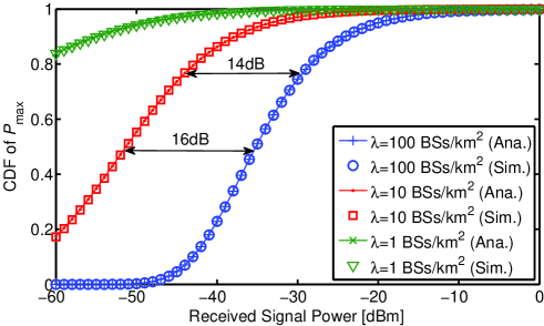
Figure 1: CDF of the strongest received signal power, $P_{t}=1$ W (30 dBm), log-normal shadowing with zero means, $\sigma^{\textrm{NL}}=4$ dB and $\sigma^{\textrm{L}}=3$ dB, simulation and analytical results.

V The Coverage Probability and ASE Analysis

In downlink performance evaluation, for networks where BSs are random distributed according to a homogeneous PPP, it is sufficient to study the performance of the typical MU located at the origin $o$ to characterize the performance of a SCN using the Palm theory [32, Eq. (4.71)]. In this section, the coverage probability and ASE are first investigated and then several special cases will be studied.

V-A General Case and Main Result

The coverage probability is generally defined as the probability that the typical MU’s measured SINR is greater than a designated threshold $T$, i.e.,

$$p_{c}\left(\lambda,T\right)=\Pr\left[\textrm{SINR}>T\right],$$ (22)

where the definition of SINR is given by Eq. (9) and the subscript $i$ is omitted here for simplicity. Now, we present a main result in this section on the coverage probability as follows.

Theorem 6 (Coverage Probability).

Given that the signal propagation model follows Eq. (8) and the typical MU selects the serving BS according to Eq. (11) or Eq. (12), then the coverage probability $p_{c}\left(\lambda,T\right)$ can be evaluated by

$$p_{c}\left(\lambda,T\right)=\stackrel{{\scriptstyle[}}{{n}}=1]{N}{\sum}p_{c,n}^{\textrm{L}}\left(\lambda,T\right)+\stackrel{{\scriptstyle[}}{{n}}=1]{N}{\sum}p_{c,n}^{\textrm{NL}}\left(\lambda,T\right),$$ (23)

where

$$p_{c,n}^{\textrm{L}}\left(\lambda,T\right)=\int_{y=0}^{\infty}\int_{\omega=-\infty}^{\infty}\left[\frac{1-e^{-j\omega/T}}{2\pi j\omega}\right]\lambda_{n}^{\textrm{L}}\left(y\right)$$

$$\quad\,\times\exp\biggl{\{}-\Lambda_{n}^{\textrm{NL}}\left(\left[0,y^{\alpha_{n}^{\textrm{L}}/\alpha_{n}^{\textrm{NL}}}\right]\right)-\Lambda_{n}^{\textrm{L}}\left(\left[0,y\right]\right)+j\omega\eta y^{\alpha_{n}^{\textrm{L}}}$$

$$\quad\,+\int_{t=y^{\alpha_{n}^{\textrm{L}}/\alpha_{n}^{\textrm{NL}}}}^{\infty}\left[e^{j\omega y^{\alpha_{n}^{\textrm{L}}}t^{-\alpha_{n}^{\textrm{NL}}}}-1\right]\lambda_{n}^{\textrm{NL}}\left(t\right)\textrm{d}t$$

$$\quad\,+\int_{t=y}^{\infty}\left[e^{j\omega\left(y/t\right)^{\alpha_{n}^{\textrm{L}}}}-1\right]\lambda_{n}^{\textrm{L}}\left(t\right)\textrm{d}t\biggr{\}}\textrm{d}\omega\textrm{d}y$$ (24)

and

$$p_{c,n}^{\textrm{NL}}\left(\lambda,T\right)=\int_{y=0}^{\infty}\int_{\omega=-\infty}^{\infty}\left[\frac{1-e^{-j\omega/T}}{2\pi j\omega}\right]\lambda_{n}^{\textrm{NL}}\left(y\right)$$

$$\quad\,\times\exp\biggl{\{}-\Lambda_{n}^{\textrm{L}}\left(\left[0,y^{\alpha_{n}^{\textrm{NL}}/\alpha_{n}^{\textrm{L}}}\right]\right)-\Lambda_{n}^{\textrm{NL}}\left(\left[0,y\right]\right)+j\omega\eta y^{\alpha_{n}^{\textrm{NL}}}$$

$$\quad\,+\int_{t=y^{\alpha_{n}^{\textrm{NL}}/\alpha_{n}^{\textrm{L}}}}^{\infty}\left[e^{j\omega y^{\alpha_{n}^{\textrm{NL}}}t^{-\alpha_{n}^{\textrm{L}}}}-1\right]\lambda_{n}^{\textrm{L}}\left(t\right)\textrm{d}t$$

$$\quad\,+\int_{t=y}^{\infty}\left[e^{j\omega\left(y/t\right)^{\alpha_{n}^{\textrm{NL}}}}-1\right]\lambda_{n}^{\textrm{NL}}\left(t\right)\textrm{d}t\biggr{\}}\textrm{d}\omega\textrm{d}y,$$ (25)

where $j=\sqrt{-1}$ denotes the imaginary unit, $\lambda_{n}^{\textrm{NL}}\left(\cdot\right)$ and $\lambda_{n}^{\textrm{L}}\left(\cdot\right)$ are defined in Theorem 2.

Proof:

See Appendix C. ∎

The coverage probability evaluated by Eq. (23) in Theorem 6 is at least a 3-fold integral which is somehow complicated for numerical computation. However, Theorem 6 gives general results that can be applied to various multi-path fading or shadowing models, e.g., Rayleigh fading, Nakagami-$m$ fading, etc, and various NLoS/LoS transmission models as well. In the following, we turn our attention to a few relevant special cases where

1. NLoS transmissions and LoS transmissions are concatenated with different shadowing, which will be studied in Subsection V-B;

2. NLoS transmissions and LoS transmissions are concatenated with Nakagami-$m$ fading of different parameters, which will be studied in Subsection V-C;

3. NLoS transmissions and LoS transmissions are concatenated with Rayleigh fading and Rician fading, respectively, which will be studied in Subsection V-D.

4. Composite Rayleigh fading, Rician fading and log-normal shadowing are considered in Subsection V-E.

V-B NLoS transmissions and LoS transmissions are concatenated with different shadowing

In the subsection, we assume that NLoS transmission and LoS transmission are concatenated with different log-normal shadowing. The association scheme is based on the SARP. Moreover, a simplified NLoS/LoS transmission model is used for a specific analysis, which is expressed by

$$p^{\textrm{L}}\left(R_{i}\right)=\begin{cases}1,&R_{i}\in\left(0,d\right]\\ 0,&R_{i}\in\left(d,\infty\right]\end{cases},$$ (26)

where $d$ is a constant distance below which all BSs connect with the typical MU with LoS transmissions. This model has been used in some recent work [14, 13]. With assumptions above, the intensity measure for NLoS transmissions, i.e., $\Lambda_{\log}^{\textrm{NL}}\left(\cdot\right)$, is expressed as follows

$$\quad\,\Lambda_{\log}^{\textrm{NL}}\left(\left[0,t\right]\right)=\mathbb{E}_{\mathcal{H}^{\textrm{NL}}}\left[2\pi\lambda\int_{R_{i}=0}^{t\left(B^{\textrm{NL}}\mathcal{H}^{\textrm{NL}}\right)^{1/\alpha^{\textrm{NL}}}}p^{\textrm{NL}}\left(R_{i}\right)R_{i}\textrm{d}R_{i}\right]$$

$$=\frac{1}{2}\pi\lambda t^{2}\left(B^{\textrm{NL}}\right)^{2/\alpha^{\textrm{NL}}}e^{1/M_{\textrm{NL}}^{2}}\textrm{erfc}\left[M_{\textrm{NL}}\ln t+Q_{\textrm{NL}}\right]$$

$$\quad\,-\frac{1}{2}\pi\lambda d^{2}\textrm{erfc}\left[M_{\textrm{NL}}\ln t+V_{\textrm{NL}}\right],$$ (27)

where $\textrm{erfc}\left(\cdot\right)$ is the complementary error function, $M_{\textrm{NL}}=-\frac{\alpha^{\textrm{NL}}}{\sqrt{2}\sigma^{\textrm{NL}}}$, $Q_{\textrm{NL}}=\frac{\alpha^{\textrm{NL}}\ln d-\ln B^{\textrm{NL}}}{\sqrt{2}\sigma^{\textrm{NL}}}-\frac{1}{M_{\textrm{NL}}}$ and $V_{\textrm{NL}}=\frac{\alpha^{\textrm{NL}}\ln d-\ln B^{\textrm{NL}}}{\sqrt{2}\sigma^{\textrm{NL}}}$ are all constants. After obtaining $\Lambda_{\log}^{\textrm{NL}}\left(\cdot\right)$, the density of NLoS BSs, i.e., $\lambda_{\log}^{\textrm{NL}}\left(\cdot\right)$, can be readily derived as follows

$$\quad\,\lambda_{\log}^{\textrm{NL}}\left(t\right)=\frac{\textrm{d}}{\textrm{d}t}\Lambda^{\textrm{NL}}\left(\left[0,t\right]\right)$$

$$=\pi\lambda t\left(B^{\textrm{NL}}\right)^{2/\alpha^{\textrm{NL}}}e^{1/M_{\textrm{NL}}^{2}}\textrm{erfc}\left[M_{\textrm{NL}}\ln t+Q_{\textrm{NL}}\right]$$

$$\quad\,+\frac{M_{\textrm{NL}}\lambda\sqrt{\pi}d^{2}}{t}e^{-\left(M_{\textrm{NL}}\ln t+V_{\textrm{NL}}\right)^{2}}$$

$$\quad\,-M_{\textrm{NL}}\lambda t\sqrt{\pi}\left(B^{\textrm{NL}}\right)^{2/\alpha^{\textrm{NL}}}e^{1/M_{\textrm{NL}}^{2}-\left(M_{\textrm{NL}}\ln t+Q_{\textrm{NL}}\right)^{2}}.$$ (28)

Similarly, the intensity measure and density for LoS BSs are

$$\Lambda_{\log}^{\textrm{L}}\left(\left[0,t\right]\right) =\frac{1}{2}\pi\lambda t^{2}\left(B^{\textrm{L}}\right)^{2/\alpha^{\textrm{L}}}e^{1/M_{\textrm{L}}^{2}}\textrm{erfc}\left[M_{\textrm{L}}\ln t+Q_{\textrm{L}}\right]$$

$$\quad\,+\frac{1}{2}\pi\lambda d^{2}\textrm{erfc}\left[-M_{\textrm{L}}\ln t+V_{\textrm{L}}\right],$$ (29)

$$\lambda_{\log}^{\textrm{L}}\left(t\right) =\pi\lambda t\left(B^{\textrm{L}}\right)^{2/\alpha^{\textrm{L}}}e^{1/M_{\textrm{L}}^{2}}\textrm{erfc}\left[M_{\textrm{L}}\ln t+Q_{\textrm{L}}\right]$$

$$\quad\,+\frac{M_{\textrm{L}}\lambda\sqrt{\pi}d^{2}}{t}e^{-\left(-M_{\textrm{L}}\ln t+V_{\textrm{L}}\right)^{2}}$$

$$\quad\,-M_{\textrm{L}}\lambda t\sqrt{\pi}\left(B^{\textrm{L}}\right)^{2/\alpha^{\textrm{L}}}e^{1/M_{\textrm{L}}^{2}-\left(M_{\textrm{L}}\ln t+Q_{\textrm{L}}\right)^{2}},$$ (30)

respectively, where $M_{\textrm{L}}=\frac{\alpha^{\textrm{L}}}{\sqrt{2}\sigma^{\textrm{L}}}$, $Q_{\textrm{L}}=\frac{\ln B^{\textrm{L}}-\alpha^{\textrm{L}}\ln d}{\sqrt{2}\sigma^{\textrm{L}}}+\frac{1}{M_{\textrm{L}}}$ and $V_{\textrm{L}}=\frac{\alpha^{\textrm{L}}\ln d-\ln B^{\textrm{L}}}{\sqrt{2}\sigma^{\textrm{L}}}$ are all constants. By substituting $\lambda_{\log}^{\textrm{NL}}\left(\cdot\right)$ and $\lambda_{\log}^{\textrm{L}}\left(\cdot\right)$ above into Eq. (24) and Eq. (25), the coverage probability can be obtained in this specific scenario, followed by results in Section VI.

In the above scenario, the shadowing follows log-normal distributions. However, Theorem 6 can also be applied to a generalized fading model and the coverage probability will be derived in the next two sections.

V-C NLoS and LoS Transmissions are Concatenated with Nakagami-$m$ Fading

Note that if we replace $\mathcal{H}^{\textrm{U}}$ by multi-path fading, i.e., $h^{\textrm{U}}$, Theorem 6 also works for the scenario where the SIRP association is applied. In this subsection, we assume that both NLoS and LoS transmissions are concatenated with Nakagami-$m$ fading of different parameters, e.g., $m^{\textrm{NL}}$ and $m^{\textrm{L}}$, then the channel power gains are distributed according to Gamma distributions. That is,

$$f_{h^{\textrm{U}}}\left(h\right)=\frac{\left(m^{\textrm{U}}\right)^{m^{\textrm{U}}}}{\Gamma\left(m^{\textrm{U}}\right)}h^{m^{\textrm{U}}-1}e^{-m^{\textrm{U}}h}.$$ (31)

By substituting the PDF of $h^{\textrm{U}}$ into Eq. (17) – Eq. (20), the intensity measures and intensities of $\overline{\Phi^{\textrm{NL}}}$ and $\overline{\Phi^{\textrm{L}}}$ can be readily obtained as follows

$$\Lambda_{\textrm{Naka}}^{\textrm{NL}}\left(\left[0,t\right]\right)=-\frac{\pi\lambda d^{2}}{\Gamma\left(m^{\textrm{NL}}\right)}\Gamma\left(m^{\textrm{NL}},\frac{m^{\textrm{NL}}}{B^{\textrm{NL}}}\left(\frac{d}{t}\right)^{\alpha^{\textrm{NL}}}\right)$$

$$+\frac{\pi\lambda t^{2}}{\Gamma\left(m^{\textrm{NL}}\right)}\left(\frac{B^{\textrm{NL}}}{m^{\textrm{NL}}}\right)^{\frac{2}{\alpha^{\textrm{NL}}}}\Gamma\left(\frac{2}{\alpha^{\textrm{NL}}}+m^{\textrm{NL}},\frac{m^{\textrm{NL}}}{B^{\textrm{NL}}}\left(\frac{d}{t}\right)^{\alpha^{\textrm{NL}}}\right),$$ (32)

$$\Lambda_{\textrm{Naka}}^{\textrm{L}}\left(\left[0,t\right]\right)=\frac{\pi\lambda d^{2}}{\Gamma\left(m^{\textrm{L}}\right)}\Gamma\left(m^{\textrm{L}},\frac{m^{\textrm{L}}}{B^{\textrm{L}}}\left(\frac{d}{t}\right)^{\alpha^{\textrm{L}}}\right)$$

$$+\frac{\pi\lambda t^{2}}{\Gamma\left(m^{\textrm{L}}\right)}\left(\frac{B^{\textrm{L}}}{m^{\textrm{L}}}\right)^{\frac{2}{\alpha^{\textrm{L}}}}\gamma\left(\frac{2}{\alpha^{\textrm{L}}}+m^{\textrm{L}},\frac{m^{\textrm{L}}}{B^{\textrm{L}}}\left(\frac{d}{t}\right)^{\alpha^{\textrm{L}}}\right),$$ (33)

$$\lambda_{\textrm{Naka}}^{\textrm{NL}}\left(t\right) =\frac{2\pi\lambda t}{\Gamma\left(m^{\textrm{NL}}\right)}\left(\frac{B^{\textrm{NL}}}{m^{\textrm{NL}}}\right)^{\frac{2}{\alpha^{\textrm{NL}}}}$$

$$\quad\,\times\Gamma\left(\frac{2}{\alpha^{\textrm{NL}}}+m^{\textrm{NL}},\frac{m^{\textrm{NL}}}{B^{\textrm{NL}}}\left(\frac{d}{t}\right)^{\alpha^{\textrm{NL}}}\right),$$ (34)

and

$$\lambda_{\textrm{Naka}}^{\textrm{L}}\left(t\right)=\frac{2\pi\lambda t}{\Gamma\left(m^{\textrm{L}}\right)}\left(\frac{B^{\textrm{L}}}{m^{\textrm{L}}}\right)^{\frac{2}{\alpha^{\textrm{L}}}}\gamma\left(\frac{2}{\alpha^{\textrm{L}}}+m^{\textrm{L}},\frac{m^{\textrm{L}}}{B^{\textrm{L}}}\left(\frac{d}{t}\right)^{\alpha^{\textrm{L}}}\right),$$ (35)

respectively, where $\Gamma\left(s,x\right)=\int_{x}^{\infty}v^{s-1}e^{-v}\textrm{d}v$ and $\gamma\left(s,x\right)=\int_{0}^{x}v^{s-1}e^{-v}\textrm{d}v$ denote the upper and the lower incomplete gamma functions, respectively, $\Gamma\left(s\right)=\int_{0}^{\infty}v^{s-1}e^{-v}\textrm{d}v$ is the gamma function. The intermediate steps are easy to derive and thus omitted here. By incorporating Eq. (32) - (35) into Eq. (24) and Eq. (25), the coverage probability of a SCN experiencing Nakagami-$m$ fading can be calculated.

V-D NLoS Transmission + Rayleigh Fading and LoS Transmission + Rician Fading

In this part, we consider a more common case in which NLoS transmission and LoS transmission are concatenated with Rayleigh fading and Rician fading, respectively, i.e., $h^{\textrm{NL}}$ follows an exponential distribution and $h^{\textrm{L}}$ follows a non-central Chi-squared distribution. With $m=\left(K+1\right)^{2}/2K+1$, Rician fading can be approximated by a Nakagami-$m$ distribution [36], where $K$ is the Rician $K$-factor representing the ratio between the power of the direct path and that of the scattered paths. Without loss of generality, we assume $f_{h^{\textrm{NL}}}\left(h\right)=e^{-h}$ and $f_{h^{\textrm{L}}}\left(h\right)=\frac{m^{m}}{\Gamma\left(m\right)}h^{m-1}e^{-mh}$ for NLoS and LoS transmissions, respectively.

As we have provided the intensity measure and intensity of $\overline{\Phi^{\textrm{L}}}$ experiencing Nakagami-$m$ fading in the previous subsection, in this part we just provide the intensity measures and intensities of $\overline{\Phi^{\textrm{NL}}}$. By substituting the PDF of $h^{\textrm{NL}}$ into Eq. (19) and Eq. (17), $\Lambda_{\textrm{Ray}}^{\textrm{NL}}\left(\left[0,t\right]\right)$ and $\lambda_{\textrm{Ray}}^{\textrm{NL}}\left(t\right)$ can be easily evaluated by

$$\Lambda_{\textrm{Ray}}^{\textrm{NL}}\left(\left[0,t\right]\right) =\pi\lambda t^{2}\left(B^{\textrm{NL}}\right)^{\frac{2}{\alpha^{\textrm{NL}}}}\Gamma\left(\frac{2}{\alpha^{\textrm{NL}}}+1,\frac{1}{B^{\textrm{NL}}}\left(\frac{d}{t}\right)^{\alpha^{\textrm{NL}}}\right)$$

$$-\pi\lambda d^{2}\exp\left[-\frac{\left(d/t\right)^{\alpha^{\textrm{NL}}}}{B^{\textrm{NL}}}\right],$$ (36)

and

$$\lambda_{\textrm{Ray}}^{\textrm{NL}}\left(t\right)=2\pi\lambda t\left(B^{\textrm{NL}}\right)^{\frac{2}{\alpha^{\textrm{NL}}}}\Gamma\left(\frac{2}{\alpha^{\textrm{NL}}}+1,\frac{1}{B^{\textrm{NL}}}\left(\frac{d}{t}\right)^{\alpha^{\textrm{NL}}}\right),$$ (37)

respectively. After substituting the intensity measures and intensities of $\overline{\Phi^{\textrm{NL}}}$ and $\overline{\Phi^{\textrm{L}}}$ into Eq. (25) and Eq. (24), the coverage probability can be obtained and we omit the rest derivations.

V-E Composite Rayleigh Fading, Rician Fading and Log-normal Shadowing

Inspired by [23] which takes composite fading into consideration, in this subsection both fading and shadowing will be considered simultaneously. In [34], a channel gain PDF which characterizes the composite effect of Rayleigh fading and log-normal shadowing is given by

$$f_{H}\left(h\right)=\frac{1}{\sqrt{2\pi\sigma_{s}^{2}}}\int_{x=0}^{\infty}\frac{1}{x^{2}}e^{-\frac{h}{x}-\frac{\left(\ln x-\mu_{s}\right)^{2}}{2\sigma_{s}^{2}}}\textrm{d}x,$$ (38)

where $\mu_{s}$ and $\sigma_{s}^{2}$ are the mean and variance of log-normal shadowing, respectively. By substituting the PDF of $H$ into Eq. (19) and Eq. (17), $\Lambda^{\textrm{NL}}\left(\left[0,t\right]\right)$ and $\lambda^{\textrm{NL}}\left(t\right)$ can be obtained, which however are non-closed forms. As for the channel model with composite Rician fading and log-normal shadowing, no such PDF could be found like Eq. (38). In this context, we utilize a simplified composite fading and shadowing channel model in which the desired signal experiences Rayleigh fading or Rician fading and the interference signal experiences log-normal shadowing [10, 37]. For example, assume that the desired NLoS transmission is concatenated with Rayleigh fading, the desired LoS transmission is concatenated with Rician fading and the aggregate interference is concatenated with log-normal shadowing. The coverage probability can be readily obtained by substituting $\lambda_{\log}^{\textrm{NL}}\left(t\right)$ into Eq. (55), $\lambda_{\log}^{\textrm{NL}}\left(t\right)$ into Eq. (56) and $\lambda_{\textrm{Ray}}^{\textrm{U}}\left(t\right)$, $\Lambda_{\textrm{Ray}}^{\textrm{U}}\left(\left[0,t\right]\right)$ into Eq. (57), respectively.

V-F The Asymptotic Analysis

In the following, an asymptotic analysis will be given for the situation where BS deployment becomes ultra-dense, i.e., $\lambda\rightarrow\infty$, which helps to analyze the performance with a concise form.

Corollary 7.

If $T\geqslant 1$, the coverage probability of $p_{c}\left(\lambda,T\right)$ considering a single-slope path loss model in Eq. (23) when $\lambda\rightarrow\infty$ converges as follows

$$\underset{\lambda\rightarrow\infty}{\lim}p_{c}\left(\lambda,T\right) =\underset{\lambda\rightarrow\infty}{\lim}\Pr\left[\textrm{SINR}>T\right]$$

$$\overset{\left(a\right)}{=}\underset{\lambda\rightarrow\infty}{\lim}\Pr\left[\textrm{SIR}>T\right]$$

$$\overset{\left(b\right)}{=}\frac{\alpha^{\textrm{L}}\sin\left(2\pi/\alpha^{\textrm{L}}\right)}{2\pi T^{2/\alpha^{\textrm{L}}}}.$$ (39)

Proof:

A sketch of the proof of Corollary 7 is given here. In Eq. (39), $\left(a\right)$ is due to the reason that when $\lambda\rightarrow\infty$, the network is interference-limited and noise can be ignored compared with the aggregate interference, which is also validated by results in Section VI. The proof of $\left(b\right)$ can be found in [11, Remark 9] and [14, Theorem 4] and are omitted here. ∎

From Corollary 7, it can be concluded that for dense SCNs the coverage probability is invariant with respect to BS density $\lambda$ and even the distribution of shadowing/fading. However, when the BS density is not dense enough, the coverage probability reveals an interesting performance, which will be fully studied in Section VI.

Moreover, when considering a multi-slope path model, when $\lambda\rightarrow\infty$, the noise power can be ignored compared with the interference and the typical MU will connected to a LoS BS almost for sure due the blockage probability model in Eq. (3). In this context,

$$\underset{\lambda\rightarrow\infty}{\lim}p_{c}\left(\lambda,T\right) =\underset{\lambda\rightarrow\infty}{\lim}\Pr\left[\textrm{SIR}>T\right]$$

$$=\underset{\lambda\rightarrow\infty}{\lim}\Pr\left[\textrm{SIR}\left(\left\{l_{n},\alpha_{n}^{\textrm{L}}\right\}\right)>T\right],$$ (40)

where $\Pr\left[\textrm{SIR}\left(\left\{l_{n},\alpha_{n}^{\textrm{L}}\right\}\right)>T\right]$ denotes the coverage probability with multi-slope path loss model ($N$ piece-wise function) but only LoS transmissions being considered. From [17, Lemma 3] and assuming that $0\leqslant\alpha_{1}^{\textrm{L}}\leqslant\alpha_{2}^{\textrm{L}}\leqslant\cdots\leqslant\alpha_{N}^{\textrm{L}}$, when $\lambda\rightarrow\infty$, the coverage probability approaches to

$$\underset{\lambda\rightarrow\infty}{\lim}p_{c}\left(\lambda,T\right) =\underset{\lambda\rightarrow\infty}{\lim}\Pr\left[\textrm{SIR}\left(\left\{l_{n},\alpha_{n}^{\textrm{L}}\right\}\right)>T\right]$$

$$=\underset{\lambda\rightarrow\infty}{\lim}\Pr\left[\textrm{SIR}\left(\left\{l_{1},\alpha_{1}^{\textrm{L}}\right\}\right)>T\right],$$ (41)

which is only determined by the first piece single-slope path loss function. As for the ASE scaling law against $\lambda$, the readers may refer to [17, 38].

V-G The ASE Upper Bound

Finally, the upper bound of ASE in units of bps/Hz/k$m^{2}$ for a given BS density $\lambda$ can be derived as follows [19]

$$\textrm{ASE}\left(\lambda\right) =\lambda\mathbb{E}_{\textrm{SINR}}\left[\log_{2}\left(1+\textrm{SINR}\right)\right]$$

$$=\lambda\int_{u=T}^{\infty}\log_{2}\left(1+u\right)f_{\textrm{SINR}}\left(\lambda,u\right)\textrm{d}u$$

$$\leqslant\lambda\int_{u=0}^{\infty}\log_{2}\left(1+u\right)f_{\textrm{SINR}}\left(\lambda,u\right)\textrm{d}u$$

$$=\frac{\lambda}{\ln 2}\int_{u=0}^{\infty}\frac{p_{c}\left(\lambda,T\right)}{u+1}\textrm{d}u,$$ (42)

where the integral in Eq. (42) can be numerically obtained [39, Eq. (10)]. Note that in [23], the proposed MGF–based approach can efficiently compute the ASE instead of obtaining the coverage probability in advance. While in our work, the coverage probability and the ASE can be analyzed simultaneously at the expense of increased complexity of computation.

VI Simulations and Discussions

This section presents numerical results to validate our analysis, followed by discussions to shed new light on the performance of SCNs. We use the following parameter values, $P_{t}=30\textrm{ dBm}$, $A^{\textrm{NL}}=30.8\textrm{ dB}$ , $A^{\textrm{L}}=2.7\textrm{ dB}$, $\alpha^{\textrm{NL}}=4.28$, $\alpha^{\textrm{L}}=2.42$, $\sigma^{\textrm{NL}}=4\textrm{ dB}$, $\sigma^{\textrm{L}}=3\textrm{ dB}$, $T=0\textrm{ dB}$ and $d=250\textrm{ m}$ [14, 13, 27, 8, 1, 40].

VI-A Validation of the Analytical Results of $p_{c}\left(\lambda,T\right)$ with Monte Carlo Simulations

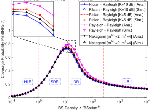
Figure 2: Coverage probability vs. BS density $\lambda$, $\eta=-95\textrm{ dBm}$, $\mu^{\textrm{NL}}=\mu^{\textrm{L}}=1$, simulation and analytical results.

The results of $p_{c}\left(\lambda,T\right)$ configured with $T=0\textrm{ dB}$ are plotted in Fig. 2 and Fig. 3, which illustrate the coverage performance of networks using SIRP and SARP, respectively. As can be observed from Fig. 2 and Fig. 3, the analytical results match the simulation results well, which validate the accuracy of our theoretical analysis. Note that in the case where both NLoS and LoS transmissions are concatenated with Rayleigh fading, the coverage probability is the highest among the interested cases. By contrast, in the case where NLoS transmission is concatenated with Rayleigh fading and LoS transmission is concatenated with Rician fading with $K=10\textrm{ dB}$, the coverage probability is the lowest, which suggests that Rayleigh fading model exaggerates network performance. Meanwhile, we should notice that the gap between the plotted curves is small, which means that multi-path fading has a minor impact on the coverage probability performance. In Fig. 3, the coverage probability with composite fading and shadowing channel model is also illustrated, which shows a similar tendency compared with others. With the assistance of Fig. 4, we conclude that the performance of small cell networks can be divided into four different regimes according to the density of small cell BSs, where in each regime, the performance is dominated by different factors. That is,

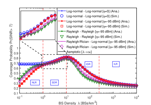
Figure 3: Coverage probability vs. BS density $\lambda$, $\mu^{\textrm{NL}}=\frac{1}{23.45}$, $\mu^{\textrm{L}}=\frac{1}{7.32}$ [13], simulation and analytical results.

• Noise-Limited Regime (NLR): ($\lambda\leqslant 1\textrm{ BSs/k$m^{2}$}$ in Fig. 3, Fig. 4 and Fig. 5). In this regime, the typical MU is likely to have a NLoS path with the serving BS, see Fig. 4 . The network in the NLR regime is very sparse and thus the interference can be ignored compared with the thermal noise if we use SINR for performance metric. In this case, $\textrm{SINR}=\frac{S}{\eta}$ and the coverage probability will increase with the increase of $\lambda$ as the strongest received power ($S$) will grow and noise power ($\eta$) will remain the same. While if we use SIR for performance metric, the SIR coverage probability remain almost stable in this regime as $\lambda$ increases. This is because the increase in the received signal power is counterbalanced by the increase in the aggregate interference power. Besides, as the aggregate interference power is smaller than noise power, the SIR coverage probability is larger than the SINR coverage probability.

• Signal-Dominated Regime (SDR): ($\lambda\in(1,10]\textrm{ BSs/k$m^{2}$}$ in Fig. 3, Fig. 4 and Fig. 5). In this regime, when $\lambda$ is small, the typical MU has a higher probability to connect to a NLoS BS; while when $\lambda$ becomes larger, the typical MU has an increasingly higher probability to connect to a LoS BS. That is to say, with the increase of $\lambda$, the typical MU is more likely to be in LoS with the associated BS, i.e., the received signal transforms from NLoS to LoS path. Even though the associated BS is LoS, the majority of interfering BSs are still NLoS in this regime and thus the SINR (or SIR) coverage probability keeps growing. From this regime on, noise power has a negligible impact on coverage performance, i.e., the SCN is interference-limited. Besides, if ignoring noise power, from the NLR to the SDR, the coverage probability from NLoS BSs decreases to almost zero and the coverage probability contributed by LoS BSs increases. It is because when the network is sparse, almost all MUs are associated with NLoS BSs and when the network goes denser, MUs shift from NLoS BSs to LoS BSs.

• Interference-Dominated Regime (IDR): ($\lambda\in(10,250]\textrm{ BSs/k$m^{2}$}$ in Fig. 3, Fig. 4 and Fig. 5). In this regime, the typical MU is connected to a LoS BS with a high probability. However, different from the situation in the SDR, the majority of interfering BSs experience transitions from NLoS to LoS path, which causes much more severe interference to the typical MU compared with interfering BSs with NLoS paths. As a result, the SINR (or SIR) coverage probability decreases with the increase of $\lambda$ because the transition of interference from NLoS path to LoS path causes a larger increase in interference compared with that in signal. Note that in this regime the coverage probability performance in our model exhibits a huge difference from that of the analysis in [10], which are indicated as “NLoS only” and “LoS only” in Fig. 5.

• Interference-Limited Regime (ILR): ($\lambda>250\textrm{ BSs/k$m^{2}$}$ in Fig. 3, Fig. 4 and Fig. 5). In this regime, the network is extremely dense and grow close to the LoS-BS-only scenario as the increase of $\lambda$. The SINR (or SIR) coverage probability will become stable with the increase in BS density as any increase in the received LoS BS signal power is counterbalanced by the increase in the aggregate LoS BS interference power, which is also illuminated by Corollary 7.

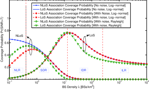
Figure 4: NLoS/LoS association coverage probability vs. BS density $\lambda$, $\mu^{\textrm{NL}}=\frac{1}{23.45}$, $\mu^{\textrm{L}}=\frac{1}{7.32}$ [13].

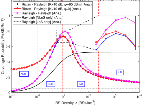
Figure 5: Coverage probability vs. BS density $\lambda$, $\mu^{\textrm{NL}}=\mu^{\textrm{L}}=1$.

To validate the four performance regimes still exist in the networks employing actual building topology. Followed by [13], we present the coverage probability of Chicago in Fig. 7 whose topology is shown in Fig. 6. Note that the NLoS transmissions and LoS transmissions are not determined by the one-parameter distance-based statistic model which is used in our work. Instead, they are determined by whether the transmission links are blocked by buildings or not. It is found that the four performance regimes still exist especially when the noise power is considered with a real building topology. The only difference is that the BS density at which the coverage probability peaks shifts from around $10\textrm{ BSs/k$m^{2}$}$ to around $100\textrm{ BSs/k$m^{2}$}$. In our work, the probability function of blockage is a piece-wise function which can be adjusted according to the real scenario.

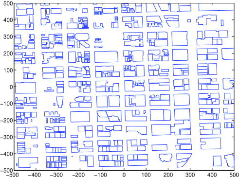
Figure 6: Building topology of Chicago.

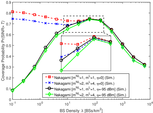
Figure 7: Coverage probability vs. BS density in Chicago.

VI-B Boundary Definitions

Based on the qualitative results above, it is interesting to develop a qualitative definition of the boundaries among adjacent regimes. In this subsection, we propose the following definition to characterize three BS density boundaries, which makes the analysis of SCNS more formal.

Definition 8.

The boundary between NLR and SDR is $\lambda_{\textrm{SDR}}^{\textrm{NLR}}$ which is defined as follows

$$\lambda_{\textrm{SDR}}^{\textrm{NLR}}=\underset{\lambda}{\arg}\left\{\mathbb{E}\left[I\right]=\eta\right\}.$$ (43)

The intuition of this definition is when $\lambda>\lambda_{\textrm{SN2LTR}}^{\textrm{NLR}}$, the aggregate interference has a greater impact on network performance than that caused by noise.

Definition 9.

The boundary between SDR and IDR is $\lambda_{\textrm{IDR}}^{\textrm{SDR}}$, which is defined as the BS density that the coverage probability achieves the highest, i.e.,

$$p_{c}^{\max}=p_{c}\left(\lambda_{\textrm{IDR}}^{\textrm{SDR}},T\right),$$ (44)

which is equivalent to $\lambda_{\textrm{IDR}}^{\textrm{SDR}}=\underset{\lambda}{\arg\max}\left\{p_{c}\left(\lambda,T\right)\right\}$. The definition above reveals that $p_{c}\left(\lambda_{\textrm{IDR}}^{\textrm{SDR}},T\right)$ is the maximum coverage probability if other parameters are fixed. From discussions above, the performance in the SDR is dominated by the desired signal, while in the IDR, the performance is dominated by the interference. When $\lambda>\lambda_{\textrm{IDR}}^{\textrm{SDR}}$, LoS interference will degrade the coverage performance.

Definition 10.

The boundary between IDR and ILR is $\lambda_{\textrm{ILR}}^{\textrm{IDR}}$, which is defined as $\forall\lambda>\lambda_{\textrm{ILR}}^{\textrm{IDR}}$

$$\mathbb{E}\left[I\right]\gg\eta,$$ (45)

which is equivalent to $\lambda_{\textrm{ILR}}^{\textrm{IDR}}=\underset{\lambda}{\arg}\left\{\mathbb{E}\left[I\right]=\epsilon\eta\right\},$ where $\epsilon\gg 1$. When $\lambda$ becomes larger and larger, the SCNs fall into the ILR, i.e., the aggregate interference might be extremely large compared with the noise power $\eta$, which is shown by Eq. (45). When $\lambda>\lambda_{\textrm{ILR}}^{\textrm{IDR}}$, the coverage changes slowly and approaches the asymptotic value. In the following, we will analyze the ASE performance in the four defined regimes.

VI-C Discussion on the Analytical Results of the Upper Bound $\textrm{ASE}\left(\lambda\right)$

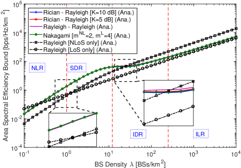
Figure 8: ASE vs. BS density $\lambda$, $\eta=-95\textrm{ dBm}$, $\mu^{\textrm{NL}}=\mu^{\textrm{L}}=1$.

In this part, the upper bound of ASE with $T=0\textrm{ dB}$ is evaluated analytically only, as the upper bound is a function of $p_{c}\left(\lambda,T\right)$ shown in Eq. (42).

Fig. 8 illustrates the upper bound with different fading models vs. $\lambda$. It is found that the upper bound of the SCN incorporating both NLoS and LoS transmissions reveal a deviation from that of the analysis considering NLoS (or LoS) transmissions only [10]. Specifically, when the SCN is sparse and thus in the NLR or the SDR, the upper bound quickly increases with $\lambda$ because the network is generally noise-limited, and thus adding more small cells immensely benefits the ASE. When the network becomes dense, i.e., $\lambda$ enters the IDR, which is the practical range of $\lambda$ for the existing 4G networks and the future 5G networks, the trend of the upper bound is very interesting. First, when $\lambda\in(10,50]\textrm{ BSs/k$m^{2}$}$, the upper bound exhibits a slowing-down in the rate of growth due to the fast decrease of the coverage probability at $\lambda\in(10,50]\textrm{ BSs/k$m^{2}$}$, as shown in Fig. 2 and Fig. 3. Second, when $\lambda>50\textrm{ BSs/k$m^{2}$}$, the upper bound will pick up the growth rate since the decrease of the coverage probability becomes a minor factor compared with the increase of $\lambda$. When the SCN is extremely dense, e.g., $\lambda$ is in the ILR, the upper bound exhibits a nearly linear trajectory with respect to $\lambda$ because both the signal power and the interference power are now LoS dominated, and thus statistically stable as explained before. Moreover, it can be observed that the change of the multi-path fading model has a minor impact on the upper bound compared with the change of the path loss model.

VI-D Discussion on the Value of Theoretical Analysis

Simulation is time consuming for $\lambda\geqslant 10^{3}\textrm{ BSs/k$m^{2}$}$ and almost infeasible for $\lambda\geqslant 10^{5}\textrm{ BSs/k$m^{2}$}$. For example, simulation for networks with $\lambda=10^{5}\textrm{ BSs/k$m^{2}$}$ needs at least $4\times 10^{5}$ BSs to get a smooth curve, which consumes almost 2 weeks for a 8 core PC. On the other hand, the computational complexity for theoretical analysis is stable for all BS densities. In this context, the theoretical analysis is useful when you want to analyze an ultra-dense network, i.e., $\lambda\geqslant 10^{5}\textrm{ BSs/k$m^{2}$}$.

Based on the findings of NLoS-to-LoS-transition, next we will introduce some guidance on how to design and manage the cellular networks in order to optimize the network performance as we evolve into dense SCNs.

As described in section VI-A and VI-C, the ASE increases almost for sure as SCNs becomes denser due to the gain of frequency reuse. In contrast, the coverage probability of SCNs will firstly increase and then decrease with the increase of BS density $\lambda$. In this context, there is a trade off between the coverage probability and the ASE in the future 5G SCNs incorporating both NLoS and LoS transmissions. While in [10], denser SCNs always provide better network performance with respect to the ASE as well as the coverage probability. It is noted that compared with the existing work [10, 13] which assume the network works either in the NLR or the ILR, our findings with more elaborate working regimes partition provide guidance for network design and optimization. A rough working regimes partition may not give useful suggestions on network performance enhancement especially in the transitional regimes between the NLR and the ILR. For example, increasing BS transmit power can improve the coverage probability in the NLR but fails in the ILR [10]. In the transitional regimes between the NLR and the ILR, we may imagine that this technique transforms form being useful to being useless. However, due to the lack of detailed features in the transitional regimes, we are still not sure whether to use this technique or not. Regarding the four performance regimes, in the following, we try to provide different techniques which can be used to enhance the network performance.

1. NLR: When the network works in the NLR, e.g., most mmWave network, the interference is not the dominate factor and the desired signal strength could be enhanced by utilizing BS power control, and directional antennas, etc.

2. SDR: In this regime, the desired signal strength is still the dominate factor. Thus the techniques used in the NLR to enhance the performance are valid as well. However, some techniques will not as useful as that in the NLR. For example, directional antenna technique may work efficiently, but BS power control technique may be not so efficient as in this regime increasing the transmit power may cause interference to other users.

3. IDR: According to the data, the current 4G network is operating in the SDR. As we deploy more and more BSs in the future to meet the skyrocketing demands on wireless data, the network will fall into the IDR. In this regime, we need elaborately design the network system including transmission techniques, medium access control (MAC) protocols and coding techniques, etc, to compensate the impair of network coverage caused by strong LoS interference. The most common MAC protocols are interference cancellation, interference avoidance, and interference control. By jointly utilizing advanced transmission techniques like beamforming techniques, multiple-input-multiple-output (MIMO), multi-antenna, coordinated multi-point (CoMP) transmissions and better coding techniques, the interference will be mitigated to an acceptable level, which benefits both the coverage probability and the ASE a lot.

4. ILR: In this regime, the coverage performance is so poor even though the ASE increases with the BS density. Techniques mentioned for IDR should be already utilized in advance to avoid entering this regime.

VII Conclusions and Future Work

In this paper, we illustrated the transition behaviors in SCNs incorporating both NLoS and LoS transmissions. Based on our analysis, the network can be divided into four regimes, i.e., the NLR, the SDR, the IDR and the ILR, where in each regime the performance is dominated by different factors. The analysis helps to understand as the BS density grows continually, which dominant factor that determines the cellular network performance and therefore provide guidance on the design and management of the cellular networks as we evolve into dense SCNs. Moreover, our work adopt a generalized shadowing/fading model, in which log-normal shadowing and/or Rayleigh fading can be treated in a unified framework.

It is noted that constant transmit power is assumed in our work, however, when the BS density, i.e., $\lambda$ is large, the BS transmit power usually decreases to reduce the inter-cell interference. In our on-going work, i.e., [41, 42], density-dependent transmit power is considered and the coverage probability and the ASE reveal a different tendency. In our future work, shadowing and multi-path fading model will be considered simultaneously which is more practical for the real network. Furthermore, heterogeneous networks (HetNets) incorporating both NLoS and LoS transmissions will also be investigated.

Appendix A: Proof of Theorem 2

Firstly, we will obtain the intensity measure $\Lambda_{n}^{\textrm{NL}}$ of $\overline{\Phi_{n}^{\textrm{NL}}}$; and then the intensity $\lambda_{n}^{\textrm{NL}}$ will be easily acquired by taking a derivation of $\Lambda_{n}^{\textrm{NL}}$. By using displacement theorem [11, 33], the point process $\overline{\Phi_{n}^{\textrm{NL}}}$ is Poisson with intensity measure

$$\quad\,\Lambda_{n}^{\textrm{NL}}\left(\left[0,t\right]\right)=\mathbb{E}_{\overline{\Phi_{n}^{\textrm{NL}}}}\left[\overline{\Phi_{n}^{\textrm{NL}}}\left[b\left(0,t\right)\right]\right]$$

$$=\int_{\mathbb{R}^{2}}\Pr\left[\overline{R_{i,n}^{\textrm{NL}}}<t\right]p^{\textrm{NL}}\left(R_{i}\right)\lambda\textrm{d}\boldsymbol{X}_{i}$$

$$=\mathbb{E}_{\mathcal{H}_{n}^{\textrm{NL}}}\left\{\int_{\mathbb{R}^{2}}\Pr\left[R_{i}<t\left(B_{n}^{\textrm{NL}}\mathcal{H}_{n}^{\textrm{NL}}\right)^{1/\alpha_{n}^{\textrm{NL}}}\right]p_{n}^{\textrm{NL}}\left(R_{i}\right)\lambda\textrm{d}\boldsymbol{X}_{i}\right\}$$

$$\overset{\left(a\right)}{=}\mathbb{E}_{\mathcal{H}_{n}^{\textrm{NL}}}\left[\int_{\theta=0}^{2\pi}\int_{R_{i}=0}^{t\left(B_{n}^{\textrm{NL}}\mathcal{H}_{n}^{\textrm{NL}}\right)^{1/\alpha_{n}^{\textrm{NL}}}}p_{n}^{\textrm{NL}}\left(R_{i}\right)\lambda R_{i}\textrm{d}R_{i}\textrm{d}\theta\right]$$

$$=\mathbb{E}_{\mathcal{H}_{n}^{\textrm{NL}}}\left[2\pi\lambda\int_{R_{i}=0}^{t\left(B_{n}^{\textrm{NL}}\mathcal{H}_{n}^{\textrm{NL}}\right)^{1/\alpha_{n}^{\textrm{NL}}}}p_{n}^{\textrm{NL}}\left(R_{i}\right)R_{i}\textrm{d}R_{i}\right],$$ (46)

where $b\left(0,t\right)$ is a ball centered at the origin $o$ with radius $t$ and $\left(a\right)$ results by converting from Cartesian to polar coordinates. Considering the distance range of $d_{n-1}<R_{i}\leqslant d_{n}$ (define $d_{0}$ and $d_{N}$ as 0 and $\infty$, respectively), the equation above should be revised as follows

$$\Lambda_{n}^{\textrm{NL}}\left(\left[0,t\right]\right) =\mathbb{E}_{\mathcal{H}_{n}^{\textrm{NL}}}\left[2\pi\lambda\int_{R_{i}=d_{n-1}}^{R_{i,\max}^{\textrm{NL}}}p_{n}^{\textrm{NL}}\left(R_{i}\right)R_{i}\textrm{d}R_{i}\right],$$ (47)

where we define $R_{i,\max}^{\textrm{NL}}=\min\left\{d_{n},t\left(B_{n}^{\textrm{NL}}\mathcal{H}_{n}^{\textrm{NL}}\right)^{1/\alpha_{n}^{\textrm{NL}}}\right\}$. Then the intensity of $\overline{\Phi_{n}^{\textrm{NL}}}$ denoted by $\lambda_{n}^{\textrm{NL}}\left(\cdot\right)$ can be given by

$$\lambda_{n}^{\textrm{NL}}\left(t\right)=\frac{\textrm{d}}{\textrm{d}t}\Lambda_{n}^{\textrm{NL}}\left(\left[0,t\right]\right).$$ (48)

Note that to ensure the intensity measure is finite for any bounded set (a set is bounded if it can be contained in a ball with a finite radius), $\mathcal{H}_{n}^{\textrm{NL}}$ has to satisfy a certain condition. As $p_{n}^{\textrm{NL}}\left(R_{i}\right)\leqslant 1$, from Eq. (47), we get an inequality as follows

$$\quad\,\Lambda_{n}^{\textrm{NL}}\left(\left[0,t\right]\right)=\mathbb{E}_{\mathcal{H}_{n}^{\textrm{NL}}}\left[2\pi\lambda\int_{d_{n-1}}^{R_{i,\max}^{\textrm{NL}}}p_{n}^{\textrm{NL}}\left(R_{i}\right)R_{i}\textrm{d}R_{i}\right]$$

$$\leqslant\mathbb{E}_{\mathcal{H}_{n}^{\textrm{NL}}}\left[2\pi\lambda\int_{0}^{R_{i,\max}^{\textrm{NL}}}R_{i}\textrm{d}R_{i}\right]$$

$$=\pi\lambda\min\left\{d_{n}^{2},t^{2}\left(B_{n}^{\textrm{NL}}\right)^{2/\alpha_{n}^{\textrm{NL}}}\mathbb{E}_{\mathcal{H}_{n}^{NL}}\left[\left(\mathcal{H}_{n}^{\textrm{NL}}\right)^{2/\alpha_{n}^{\textrm{NL}}}\right]\right\}.$$ (49)

If the expectation $\mathbb{E}_{\mathcal{H}_{n}^{\textrm{NL}}}\left[\left(\mathcal{H}_{n}^{\textrm{NL}}\right)^{2/\alpha_{n}^{\textrm{NL}}}\right]<\infty$, then $\Lambda_{n}^{\textrm{NL}}\left(\left[0,t\right]\right)<\infty$. Using similar approach, the intensity measure and intensity of the PPP $\overline{\Phi_{n}^{\textrm{L}}}$ are obtained by Eq. (20) and Eq. (18), respectively.

As for the cell association scheme, it is obvious that the original scheme $\left(\boldsymbol{X}_{i},\textrm{U},\mathcal{N}\right)^{*}=\arg\underset{(\boldsymbol{X}_{i},\textrm{U},\mathcal{N})\in\mathbb{S}}{\max}B_{n}^{\textrm{U}}\mathcal{H}_{n}^{\textrm{U}}\left(R_{i}\right)^{-\alpha_{n}^{\textrm{U}}}$ is equivalent to the scheme $\left(\boldsymbol{X}_{i},\textrm{U},\mathcal{N}\right)^{*}=\arg\underset{(\boldsymbol{X}_{i},\textrm{U},\mathcal{N})\in\mathbb{S}}{\max}\left(\overline{R_{i,n}}\right)^{-\alpha_{n}^{\textrm{U}}}$ which actually corresponds to the nearest BS association scheme. Thus the proof is completed.

Appendix B: Proof of Lemma 5

Denote the strongest NLoS received signal power and the strongest LoS received signal power by $\mathcal{P}^{\textrm{NL}}$ and $\mathcal{P}^{\textrm{L}}$, respectively. Note that we drop subscript $n$ under this special case for simplicity. That is, $\mathcal{P}^{\textrm{NL}}=\max\left(P_{i}^{\textrm{NL}}\right)$ and $\mathcal{P}^{\textrm{L}}=\max\left(P_{i}^{\textrm{L}}\right)$. Then the probability $\Pr\left[\mathcal{P}\leqslant\gamma\right]$ can be derived as

$$\quad\,\Pr\left[\mathcal{P}\leqslant\gamma\right]$$

$$=\Pr\left[\max\left(\overline{R_{i}^{\textrm{NL}}}^{-\alpha^{\textrm{NL}}}\right)\leqslant\gamma\cap\max\left(\overline{R_{i}^{\textrm{L}}}^{-\alpha^{\textrm{L}}}\right)\leqslant\gamma\right]$$

$$=\Pr\left[\min\left(\overline{R_{i}^{\textrm{NL}}}\right)\geqslant\gamma^{-1/\alpha^{\textrm{NL}}}\cap\min\left(\overline{R_{i}^{\textrm{L}}}\right)\geqslant\gamma^{-1/\alpha^{\textrm{L}}}\right]$$

$$=\Pr\left[\textrm{no nodes within }\gamma^{-1/\alpha^{\textrm{NL}}}\cap\textrm{no nodes within }\gamma^{-1/\alpha^{\textrm{L}}}\right]$$

$$=\Pr\left[\overline{\Phi^{\textrm{NL}}}\left(b\left(0,\gamma^{-1/\alpha^{\textrm{NL}}}\right)\right)=0\cap\overline{\Phi^{\textrm{L}}}\left(b\left(0,\gamma^{-1/\alpha^{\textrm{L}}}\right)\right)=0\right]$$

$$\overset{\left(a\right)}{=}\Pr\left[\overline{\Phi^{\textrm{NL}}}\left(b\left(0,\gamma^{-1/\alpha^{\textrm{NL}}}\right)\right)=0\right]$$

$$\quad\,\times\Pr\left[\overline{\Phi^{\textrm{L}}}\left(b\left(0,\gamma^{-1/\alpha^{\textrm{L}}}\right)\right)=0\right]$$

$$\overset{\left(b\right)}{=}\exp\left[-\Lambda^{\textrm{NL}}\left(\left[0,\gamma^{-1/\alpha^{\textrm{NL}}}\right]\right)\right]\cdot\exp\left[-\Lambda^{\textrm{L}}\left(\left[0,\gamma^{-1/\alpha^{\textrm{L}}}\right]\right)\right],$$ (50)

where the notation $\overline{\Phi^{\textrm{U}}}\left(\Xi\right)$ refers to the number of points $x\in\overline{\Phi^{\textrm{U}}}$ contained in the set $\Xi$, while equality $\left(a\right)$ follows from the independence of PPP $\overline{\Phi^{\textrm{NL}}}$ and PPP $\overline{\Phi^{\textrm{L}}}$ , and $\left(b\right)$ comes from the fact that the void probability $\Pr\left[\overline{\Phi^{\textrm{U}}}\left(b\left(0,r\right)\right)=0\right]=\exp\left[-\Lambda^{\textrm{U}}\left(\left[0,r\right]\right)\right]$ for a non-homogeneous PPP. Then the rest of the proof is straightforward.

Appendix C: Proof of Theorem 6

By invoking the law of total probability and considering the independence between $\overline{\Phi_{n}^{\textrm{NL}}}$ and $\overline{\Phi_{n}^{\textrm{L}}}$, the coverage probability can be divided into two parts in each segment, i.e., $p_{c,n}^{\textrm{NL}}\left(\lambda,T\right)$ and $p_{c,n}^{\textrm{L}}\left(\lambda,T\right)$, which denotes the conditional coverage probability given that the typical MU is associated with a BS in $\Phi_{n}^{\textrm{NL}}$ and $\Phi_{n}^{\textrm{L}}$, respectively. Moreover, denote by $\mathcal{P}_{n}^{\textrm{NL}}$ and $\mathcal{P}_{n}^{\textrm{L}}$ the strongest received signal power from BS in $\Phi_{n}^{\textrm{NL}}$ and $\Phi_{n}^{\textrm{L}}$, i.e., $\mathcal{P}_{n}^{\textrm{NL}}=\max\left(P_{i,n}^{\textrm{NL}}\right)$ and $\mathcal{P}_{n}^{\textrm{L}}=\max\left(P_{i,n}^{\textrm{L}}\right)$, respectively. Then by applying the law of total probability, $p_{c,n}^{\textrm{L}}\left(\lambda,T\right)$ can be computed by

$$p_{c,n}^{\textrm{L}}\left(\lambda,T\right) =\Pr\left[\left(\textrm{SINR}_{n}^{\textrm{L}}>T\right)\cap\left(\mathcal{P}_{n}^{\textrm{L}}>\mathcal{P}_{n}^{\textrm{NL}}\right)\cap\mathcal{Y}_{n}^{\textrm{L}}\right]$$

$$=\mathbb{E}_{\mathcal{Y}_{n}^{\textrm{L}}}\biggl{\{}\underset{\textrm{II}}{\underbrace{\Pr\left[\left.\textrm{SINR}_{n}^{\textrm{L}}>T\right|\left(\mathcal{P}_{n}^{\textrm{L}}>\mathcal{P}_{n}^{\textrm{NL}}\right)\cap\mathcal{Y}_{n}^{\textrm{L}}\right]}}$$

$$\quad\,\times\underset{\textrm{I}}{\underbrace{\Pr\left[\left.\mathcal{P}_{n}^{\textrm{L}}>\mathcal{P}_{n}^{\textrm{NL}}\right|\mathcal{Y}_{n}^{\textrm{L}}\right]}}\biggr{\}},$$ (51)

where $\mathcal{Y}_{n}^{\textrm{L}}$ is the equivalent distance between the typical MU and the BS providing the strongest received signal power to the typical MU in $\Phi_{n}^{\textrm{L}}$, i.e., $\mathcal{Y}_{n}^{\textrm{L}}=\underset{\overline{R_{i,n}^{\textrm{L}}}\in\overline{\Phi_{n}^{\textrm{L}}}}{\arg\max}\left(\overline{R_{i,n}^{\textrm{L}}}\right)^{-\alpha_{n}^{\textrm{L}}}$, and also note that $\mathcal{P}_{n}^{\textrm{L}}=\left(\mathcal{Y}_{n}^{\textrm{L}}\right)^{-\alpha_{n}^{\textrm{L}}}$. Besides, Part I guarantees that the typical MU is connected to a LoS BS and Part II denotes the coverage probability conditioned on the proposed cell association scheme in Eq. (11). Next, Part I and Part II will be respectively derived as follows. For Part I,

$$\quad\,\Pr\left[\left.\mathcal{P}_{n}^{\textrm{L}}>\mathcal{P}_{n}^{\textrm{NL}}\right|\mathcal{Y}_{n}^{\textrm{L}}\right]$$

$$=\Pr\left[\left.\left(\mathcal{Y}_{n}^{\textrm{L}}\right)^{-\alpha_{n}^{\textrm{L}}}>\left(\mathcal{Y}_{n}^{\textrm{NL}}\right)^{-\alpha_{n}^{\textrm{NL}}}\right|\mathcal{Y}_{n}^{\textrm{L}}\right]$$

$$\overset{\left(a\right)}{=}\exp\left[-\Lambda_{n}^{\textrm{NL}}\left(\left[0,\left(\mathcal{Y}_{n}^{\textrm{L}}\right)^{\alpha_{n}^{\textrm{L}}/\alpha_{n}^{\textrm{NL}}}\right]\right)\right],$$ (52)

where $\mathcal{Y}_{n}^{\textrm{NL}}$, similar to the definition of $\mathcal{Y}_{n}^{\textrm{L}}$, is the equivalent distance between the typical MU and the BS providing the strongest received signal power to the typical MU in $\Phi_{n}^{\textrm{NL}}$, i.e., $\mathcal{Y}_{n}^{\textrm{NL}}=\underset{\overline{R_{i,n}^{\textrm{NL}}}\in\overline{\Phi_{n}^{\textrm{NL}}}}{\arg\max}\left(\overline{R_{i,n}^{\textrm{NL}}}\right)^{-\alpha_{n}^{\textrm{NL}}}$, and also note that $\mathcal{P}_{n}^{\textrm{NL}}=\left(\mathcal{Y}_{n}^{\textrm{NL}}\right)^{-\alpha_{n}^{\textrm{NL}}}$, and $\left(a\right)$ follows from the void probability of a PPP.

For Part II, we know that $\textrm{SINR}=\frac{\mathcal{P}}{I+\eta}=\frac{\mathcal{P}}{I^{\textrm{NL}}+I^{\textrm{L}}+\eta},$ where $I^{\textrm{NL}}$ and $I^{\textrm{L}}$ denote the aggregate interference from NLoS BSs and LoS BSs, respectively. The conditional coverage probability is derived as follows

$$\quad\,\Pr\left[\left.\textrm{SINR}_{n}^{\textrm{L}}>T\right|\left(\mathcal{P}_{n}^{\textrm{L}}>\mathcal{P}_{n}^{\textrm{NL}}\right)\cap\mathcal{Y}_{n}^{\textrm{L}}\right]$$

$$=\Pr\left[\left.\frac{1}{\textrm{SINR}_{n}^{\textrm{L}}}<\frac{1}{T}\right|\left(\mathcal{P}_{n}^{\textrm{L}}>\mathcal{P}_{n}^{\textrm{NL}}\right)\cap\mathcal{Y}_{n}^{\textrm{L}}\right]$$

$$\overset{\left(a\right)}{=}\underset{\textrm{PDF}}{\int_{x=0}^{1/T}\underbrace{\int_{\omega=-\infty}^{\infty}\frac{e^{-j\omega x}}{2\pi}\mathcal{F}_{\frac{1}{\textrm{SINR}_{n}^{\textrm{L}}}}\left(\omega\right)\textrm{d}\omega}\textrm{d}x}$$

$$=\int_{\omega=-\infty}^{\infty}\left[\frac{1-e^{-j\omega/T}}{2\pi j\omega}\right]\mathcal{F}_{\frac{1}{\textrm{SINR}_{n}^{\textrm{L}}}}\left(\omega\right)\textrm{d}\omega,$$ (53)

where $\textrm{SINR}_{n}^{\textrm{L}}$ denotes the SINR when the typical MU is associated with a LoS BS, the inner integral in $\left(a\right)$, i.e., $\int_{\omega=-\infty}^{\infty}\frac{e^{-j\omega x}}{2\pi}\mathcal{F}_{\frac{1}{\textrm{SINR}_{n}^{\textrm{L}}}}\left(\omega\right)\textrm{d}\omega$ is the conditional PDF of $\frac{1}{\textrm{SINR}_{n}^{\textrm{L}}}$ due to the definition of the inverse characteristic function, i.e., $f_{X}\left(x\right)=F_{X}^{{}^{\prime}}\left(x\right)=\frac{1}{2\pi}\int_{\mathrm{R}}e^{-j\omega x}\varphi_{X}\left(\omega\right)\textrm{d}\omega$, and $\mathcal{F}_{\frac{1}{\textrm{SINR}_{n}^{\textrm{L}}}}\left(\omega\right)$ denotes the conditional characteristic function of $\frac{1}{\textrm{SINR}_{n}^{\textrm{L}}}$ which is given by

$$\mathcal{F}_{\frac{1}{\textrm{SINR}_{n}^{\textrm{L}}}}\left(\omega\right)=\mathbb{E}_{\Phi_{n}}\left[\left.\exp\left(j\omega\frac{1}{\textrm{SINR}_{n}^{\textrm{L}}}\right)\right|\left(\mathcal{P}_{n}^{\textrm{L}}>\mathcal{P}_{n}^{\textrm{NL}}\right)\cap\mathcal{Y}_{n}^{\textrm{L}}\right]$$

$$=\mathbb{E}_{\Phi_{n}}\left[\left.\exp\left(j\omega\frac{I^{\textrm{NL}}+I^{\textrm{L}}+\eta}{\mathcal{P}_{n}^{\textrm{L}}}\right)\right|\left(\mathcal{P}_{n}^{\textrm{L}}>\mathcal{P}_{n}^{\textrm{NL}}\right)\cap\mathcal{Y}_{n}^{\textrm{L}}\right]$$

$$=\mathbb{E}_{\Phi_{n}}\left\{\left.\exp\left[j\omega\left(I^{\textrm{NL}}+I^{\textrm{L}}+\eta\right)\left(\mathcal{Y}_{n}^{\textrm{L}}\right)^{\alpha_{n}^{\textrm{L}}}\right]\right|\left(\mathcal{P}_{n}^{\textrm{L}}>\mathcal{P}_{n}^{\textrm{NL}}\right)\cap\mathcal{Y}_{n}^{\textrm{L}}\right\}$$

$$\overset{\left(a\right)}{=}\underset{\textrm{III}}{\underbrace{\mathbb{E}_{\Phi_{n}^{\textrm{NL}}}\left\{\left.\exp\left[j\omega I^{\textrm{NL}}\cdot\left(\mathcal{Y}_{n}^{\textrm{L}}\right)^{\alpha_{n}^{\textrm{L}}}\right]\right|\left(\mathcal{P}_{n}^{\textrm{L}}>\mathcal{P}_{n}^{\textrm{NL}}\right)\cap\mathcal{Y}_{n}^{\textrm{L}}\right\}}}$$

$$\quad\,\times\underset{\textrm{IV}}{\underbrace{\mathbb{E}_{\Phi_{n}^{\textrm{L}}}\left\{\left.\exp\left[j\omega I^{\textrm{L}}\cdot\left(\mathcal{Y}_{n}^{\textrm{L}}\right)^{\alpha_{n}^{\textrm{L}}}\right]\right|\left(\mathcal{P}_{n}^{\textrm{L}}>\mathcal{P}_{n}^{\textrm{NL}}\right)\cap\mathcal{Y}_{n}^{\textrm{L}}\right\}}}$$

$$\quad\,\times e^{j\omega\eta\left(\mathcal{Y}_{n}^{\textrm{L}}\right)^{\alpha_{n}^{\textrm{L}}}},$$ (54)

where $\left(a\right)$ comes from the facts that $\Phi_{n}=\Phi_{n}^{\textrm{NL}}\cup\Phi_{n}^{\textrm{L}}$ and the mutual independence of $\Phi_{n}^{\textrm{NL}}$ and $\Phi_{n}^{\textrm{L}}$. Now by applying stochastic geometry, we will derive the term III in Eq. (54) as follows

$$\quad\,\mathbb{E}_{\Phi_{n}^{\textrm{NL}}}\left\{\left.\exp\left[j\omega I^{\textrm{NL}}\cdot\left(\mathcal{Y}_{n}^{\textrm{L}}\right)^{\alpha_{n}^{\textrm{L}}}\right]\right|\left(\mathcal{P}_{n}^{\textrm{L}}>\mathcal{P}_{n}^{\textrm{NL}}\right)\cap\mathcal{Y}_{n}^{\textrm{L}}\right\}$$

$$\overset{\left(a\right)}{=}\mathbb{E}_{\overline{\Phi_{n}^{\textrm{NL}}}}\Biggl{\{}\left.\exp\left[j\omega\cdot\left(\mathcal{Y}_{n}^{\textrm{L}}\right)^{\alpha_{n}^{\textrm{L}}}\underset{i:\overline{R_{i,n}^{\textrm{NL}}}\in\overline{\Phi_{n}^{\textrm{NL}}}^{\prime}}{\sum}\left(\overline{R_{i,n}^{\textrm{NL}}}\right)^{-\alpha_{n}^{\textrm{NL}}}\right]\right|\bigl{(}\mathcal{P}_{n}^{\textrm{L}}$$

$$\quad\,>\mathcal{P}_{n}^{\textrm{NL}}\bigr{)}\cap\mathcal{Y}_{n}^{\textrm{L}}\Biggr{\}}$$

$$\overset{\left(b\right)}{=}\mathbb{E}_{\overline{\Phi_{n}^{\textrm{NL}}}}\Biggl{\{}\left.\underset{i:\overline{R_{i,n}^{\textrm{NL}}}\in\overline{\Phi_{n}^{\textrm{NL}}}^{\prime}}{\prod}\exp\left[j\omega\cdot\left(\mathcal{Y}_{n}^{\textrm{L}}\right)^{\alpha_{n}^{\textrm{L}}}\left(\overline{R_{i,n}^{\textrm{NL}}}\right)^{-\alpha_{n}^{\textrm{NL}}}\right]\right|\bigl{(}\mathcal{P}_{n}^{\textrm{L}}$$

$$\quad\,>\mathcal{P}_{n}^{\textrm{NL}}\bigr{)}\cap\mathcal{Y}_{n}^{\textrm{L}}\Biggr{\}}$$

$$\overset{\left(c\right)}{=}\exp\left\{\int_{t=\left(\mathcal{Y}_{n}^{\textrm{L}}\right)^{\alpha_{n}^{\textrm{L}}/\alpha_{n}^{\textrm{NL}}}}^{\infty}\left[e^{j\omega\left(\mathcal{Y}_{n}^{\textrm{L}}\right)^{\alpha_{n}^{\textrm{L}}}t^{-\alpha_{n}^{\textrm{NL}}}}-1\right]\lambda_{n}^{\textrm{NL}}\left(t\right)\textrm{d}t\right\},$$ (55)

where in $\left(a\right)$, $\overline{\Phi_{n}^{\textrm{NL}}}^{\prime}=\overline{\Phi_{n}^{\textrm{NL}}}\setminus b\left(0,\left(\mathcal{Y}_{n}^{\textrm{L}}\right)^{\alpha_{n}^{\textrm{L}}/\alpha_{n}^{\textrm{NL}}}\right)$ and $\overline{R_{i,n}^{\textrm{NL}}}\in\overline{\Phi_{n}^{\textrm{NL}}}^{\prime}$ can guarantee the condition that $\mathcal{P}_{n}^{\textrm{L}}>\mathcal{P}_{n}^{\textrm{NL}}$, $\left(b\right)$ follows from rewriting the exponential of summation as a product of several exponential functions, and $\left(c\right)$ is obtained by applying the probability generating functional (PGFL) [10, Eq. (3)] of the PPP. Similarly, the term IV in Eq. (54) is given by

$$\quad\,\mathbb{E}_{\Phi_{n}^{\textrm{L}}}\left\{\left.\exp\left[j\omega I^{\textrm{L}}\cdot\left(\mathcal{Y}_{n}^{\textrm{L}}\right)^{\alpha_{n}^{\textrm{L}}}\right]\right|\left(\mathcal{P}_{n}^{\textrm{L}}>\mathcal{P}_{n}^{\textrm{NL}}\right)\cap\mathcal{Y}_{n}^{\textrm{L}}\right\}$$

$$\overset{\left(a\right)}{=}\mathbb{E}_{\overline{\Phi_{n}^{\textrm{L}}}}\Biggl{\{}\left.\exp\left[j\omega\cdot\left(\mathcal{Y}_{n}^{\textrm{L}}\right)^{\alpha_{n}^{\textrm{L}}}\underset{i:\overline{R_{i,n}^{\textrm{L}}}\in\overline{\Phi_{n}^{\textrm{L}}}^{\prime}}{\sum}\left(\overline{R_{i,n}^{\textrm{L}}}\right)^{-\alpha_{n}^{\textrm{L}}}\right]\right|\bigl{(}\mathcal{P}_{n}^{\textrm{L}}$$

$$\quad\,>\mathcal{P}_{n}^{\textrm{NL}}\bigr{)}\cap\mathcal{Y}_{n}^{\textrm{L}}\Biggr{\}}$$

$$=\mathbb{E}_{\overline{\Phi_{n}^{\textrm{NL}}}}\Biggl{\{}\left.\underset{i:\overline{R_{i,n}^{\textrm{L}}}\in\overline{\Phi_{n}^{\textrm{L}}}^{\prime}}{\prod}\exp\left[j\omega\cdot\left(\mathcal{Y}_{n}^{\textrm{L}}/\overline{R_{i,n}^{\textrm{L}}}\right)^{\alpha_{n}^{\textrm{L}}}\right]\right|\bigl{(}\mathcal{P}_{n}^{\textrm{L}}$$

$$\quad\,>\mathcal{P}_{n}^{\textrm{NL}}\bigr{)}\cap\mathcal{Y}_{n}^{\textrm{L}}\Biggr{\}}$$

$$=\exp\left\{\int_{t=\mathcal{Y}_{n}^{\textrm{L}}}^{\infty}\left[e^{j\omega\left(\mathcal{Y}_{n}^{\textrm{L}}/t\right)^{\alpha_{n}^{\textrm{L}}}}-1\right]\lambda_{n}^{\textrm{L}}\left(t\right)\textrm{d}t\right\},$$ (56)

where in $\left(a\right)$, $\overline{\Phi_{n}^{\textrm{L}}}^{\prime}=\overline{\Phi_{n}^{\textrm{L}}}\setminus b\left(0,\mathcal{Y}_{n}^{\textrm{L}}\right)$ and $\overline{R_{i,n}^{\textrm{L}}}\in\overline{\Phi_{n}^{\textrm{L}}}^{\prime}$ can guarantee that the typical MU is associated with a LoS BS providing the strongest received signal power. Then the product of Part I and Part II in Eq. (51) can be obtained by substituting them with Eq. (52) – (56).

Finally, note that the value of $p_{c,n}^{\textrm{L}}\left(\lambda,T\right)$ in Eq. (51) should be calculated by taking the expectation with respect to $\mathcal{Y}_{n}^{\textrm{L}}$ in terms of its PDF, which is given as follows

$$f_{\mathcal{Y}_{n}^{\textrm{L}}}\left(y\right)=\frac{\textrm{d}}{\textrm{d}y}\left[1-\Pr\left(\mathcal{Y}_{n}^{\textrm{L}}>y\right)\right] =\lambda_{n}^{\textrm{L}}\left(y\right)\exp\left[-\Lambda_{n}^{\textrm{L}}\left(\left[0,y\right]\right)\right].$$ (57)

Given that the typical MU is connected to a NLoS BS, the conditional coverage probability $p_{c,n}^{\textrm{NL}}\left(\lambda,T\right)$ can be derived in a similar way as the above. In this way, the coverage probability is obtained by $p_{c}\left(\lambda,T\right)=\stackrel{{\scriptstyle[}}{{n}}=1]{N}{\sum}p_{c,n}^{\textrm{L}}\left(\lambda,T\right)+\stackrel{{\scriptstyle[}}{{n}}=1]{N}{\sum}p_{c,n}^{\textrm{NL}}\left(\lambda,T\right)$. Thus the proof is completed.

References

- [1] B. Yang, M. Ding, G. Mao, and X. Ge, “Performance analysis of dense small cell networks with generalized fading,” in Proc. IEEE ICC 2017, pp. 1–7.
- [2] W. Webb, Wireless Communications: The Future. Hoboken, NJ, USA: 1097 Wiley, 2007.
- [3] D. Lopez-Perez, M. Ding, H. Claussen, and A. H. Jafari, “Towards 1 gbps/ue in cellular systems: Understanding ultra-dense small cell deployments,” IEEE Commun. Surv. Tut., vol. 17, no. 4, pp. 2078–2101, Nov. 2015.
- [4] J. G. Andrews, S. Buzzi, C. Wan, S. V. Hanly, A. Lozano, A. C. K. Soong, and J. C. Zhang, “What will 5g be?” IEEE J. Sel. Areas Commun., vol. 32, no. 6, pp. 1065–1082, Jun. 2014.
- [5] Cisco, “Global mobile data traffic forecast update, 2015-2020,” Cisco white paper, Feb. 2016.
- [6] X. Ge, S. Tu, G. Mao, C. X. Wang, and T. Han, “5g ultra-dense cellular networks,” IEEE Wireless Commun., vol. 23, no. 1, pp. 72–79, Feb. 2016.
- [7] X. Ge, S. Tu, T. Han, Q. Li, and G. Mao, “Energy efficiency of small cell backhaul networks based on gauss-markov mobile models,” IET Networks, vol. 4, no. 2, pp. 158–167, Mar. 2015.
- [8] B. Yang, G. Mao, X. Ge, H. H. Chen, T. Han, and X. Zhang, “Coverage analysis of heterogeneous cellular networks in urban areas,” in Proc. IEEE ICC, May 2016, pp. 1–6.
- [9] B. Yang, G. Mao, X. Ge, and T. Han, “A new cell association scheme in heterogeneous networks,” in Proc. IEEE ICC 2015, June 2015, pp. 5627–5632.
- [10] J. G. Andrews, F. Baccelli, and R. K. Ganti, “A tractable approach to coverage and rate in cellular networks,” IEEE Trans. Commun., vol. 59, no. 11, pp. 3122–3134, Nov. 2011.
- [11] B. Blaszczyszyn, M. K. Karray, and H. P. Keeler, “Using poisson processes to model lattice cellular networks,” in Proc. IEEE INFOCOM, Apr. 2013, pp. 773–781.
- [12] H. S. Dhillon and J. G. Andrews, “Downlink rate distribution in heterogeneous cellular networks under generalized cell selection,” IEEE Wireless Commun. Lett., vol. 3, no. 1, pp. 42–45, Feb. 2014.
- [13] S. Singh, M. N. Kulkarni, A. Ghosh, and J. G. Andrews, “Tractable model for rate in self-backhauled millimeter wave cellular networks,” IEEE J. Sel. Areas Commun., vol. 33, no. 10, pp. 2196–2211, Oct. 2015.
- [14] T. Bai and R. W. Heath, “Coverage and rate analysis for millimeter-wave cellular networks,” IEEE Trans. Wireless Commun., vol. 14, no. 2, pp. 1100–1114, Feb. 2015.
- [15] J. Liu, M. Sheng, L. Liu, and J. Li, “Effect of densification on cellular network performance with bounded pathloss model,” IEEE Commun. Lett., vol. 21, no. 2, pp. 346–349, Feb. 2017.
- [16] A. R. Khamesi, B. Yang, X. Ge, and M. Zorzi, “Energy and spatial spectral efficiency analysis of random mimo cellular networks,” in Proc. European Wireless 2016, May 2016, pp. 1–6.
- [17] X. Zhang and J. G. Andrews, “Downlink cellular network analysis with multi-slope path loss models,” IEEE Trans. Commun., vol. 63, no. 5, pp. 1881–1894, May 2015.
- [18] H. Shokri-Ghadikolaei and C. Fischione, “The transitional behavior of interference in millimeter wave networks and its impact on medium access control,” IEEE Trans. Commun., vol. 64, no. 2, pp. 723–740, Feb. 2016.
- [19] M. Ding, P. Wang, D. Lopez-Perez, G. Mao, and Z. Lin, “Performance impact of los and nlos transmissions in dense cellular networks,” IEEE Trans. Wireless Commun., vol. 15, no. 3, pp. 2365–2380, Mar. 2016.
- [20] M. D. Renzo, “Stochastic geometry modeling and analysis of multi-tier millimeter wave cellular networks,” IEEE Trans. Wireless Commun., vol. 14, no. 9, pp. 5038–5057, Sep. 2015.
- [21] J. Arnau, I. Atzeni, and M. Kountouris, “Impact of los/nlos propagation and path loss in ultra-dense cellular networks,” in Proc. IEEE ICC, May 2016, pp. 1–6.
- [22] M. D. Renzo, W. Lu, and P. Guan, “The intensity matching approach: A tractable stochastic geometry approximation to system-level analysis of cellular networks,” IEEE Trans. Wireless Commun., vol. 15, no. 9, pp. 5963–5983, Sep. 2016.
- [23] M. D. Renzo, A. Guidotti, and G. E. Corazza, “Average rate of downlink heterogeneous cellular networks over generalized fading channels: A stochastic geometry approach,” IEEE Trans. Commun., vol. 61, no. 7, pp. 3050–3071, Jul. 2013.
- [24] X. Ge, B. Yang, J. Ye, G. Mao, and Q. Li, “Performance analysis of poisson-voronoi tessellated random cellular networks using markov chains,” in Proc. IEEE Globecom 2014, Dec. 2014, pp. 4635–4640.
- [25] N. Blaunstein and M. Levin, “Parametric model of uhf/l-wave propagation in city with randomly distributed buildings,” in Proc. IEEE Antennas and Propagation Society International Symposium, vol. 3, Jun. 1998, pp. 1684–1687.
- [26] T. Bai, R. Vaze, and R. W. Heath, “Analysis of blockage effects on urban cellular networks,” IEEE Trans. Wireless Commun., vol. 13, no. 9, pp. 5070–5083, Sep. 2014.
- [27] 3GPP, “Tr 36.828 (v11.0.0): Further enhancements to lte time division duplex (tdd) for downlink-uplink (dl-ul) interference management and traffic adaptation,” Jun. 2012.
- [28] Spatial Channel Model AHG. (2003, Apr.). Subsection 3.5.3, Spatial Channel Model Text Description V6.0, Available: http://ftp://www.3gpp.org/tsg_ran/WG1_RL1/3GPP_3GPP2_SCM/ConfCall-16-20030417/SCM-134%20Text%20v6.0.zip.
- [29] G. Mao, B. D. O. Anderson, and B. Fidan, “Online calibration of path loss exponent in wireless sensor networks,” in Proc. IEEE Globecom 2006, pp. 1–6.
- [30] G. Mao and B. D. O. Anderson, “Graph theoretic models and tools for the analysis of dynamic wireless multihop networks,” in Proc. IEEE WCNC 2009, pp. 1–6.
- [31] R. Mao and G. Mao, “Road traffic density estimation in vehicular networks,” in Proc. IEEE WCNC 2013, pp. 4653–4658.
- [32] S. N. Chiu, D. Stoyan, W. S. Kendall, and J. Mecke, Stochastic geometry and its applications. John Wiley & Sons, 2013.
- [33] F. Baccelli and B. Blaszczyszyn, Stochastic geometry and wireless networks. Now Publishers Inc, 2009.
- [34] C. H. Liu and L. C. Wang, “Optimal cell load and throughput in green small cell networks with generalized cell association,” IEEE J. Sel. Areas Commun., vol. 34, no. 5, pp. 1058–1072, May 2016.
- [35] B. Blaszczyszyn and H. P. Keeler, “Studying the sinr process of the typical user in poisson networks using its factorial moment measures,” IEEE Trans. Inf. Theory, vol. 61, no. 12, pp. 6774–6794, Dec., 2015.
- [36] A. Goldsmith, Wireless communications. Cambridge University Press, 2005.
- [37] X. Ge, B. Yang, J. Ye, G. Mao, C. X. Wang, and T. Han, “Spatial spectrum and energy efficiency of random cellular networks,” IEEE Trans. Commun., vol. 63, no. 3, pp. 1019–1030, Mar. 2015.
- [38] V. M. Nguyen and M. Kountouris, “Performance limits of network densification,” IEEE J. Sel. Areas Commun., vol. 35, no. 6, pp. 1294–1308, Jun. 2017.
- [39] F. Yilmaz and M. S. Alouini, “A unified mgf-based capacity analysis of diversity combiners over generalized fading channels,” IEEE Trans. Commun., vol. 60, no. 3, pp. 862–875, Mar. 2012.
- [40] X. Ge, J. Martínez-Bauset, V. Casares-Giner, B. Yang, J. Ye, and M. Chen, “Modelling and performance analysis of different access schemes in two-tier wireless networks,” in Proc. IEEE Globecom 2013, Dec. 2013, pp. 4402–4407.
- [41] M. Ding, D. Lopez-Perez, G. Mao, and Z. Lin, “Performance impact of idle mode capability on dense small cell networks,” Mar. 2017. Available at: https://arxiv.org/abs/1609.07710v4.
- [42] B. Yang, G. Mao, X. Ge, M. Ding, and X. Yang, “On the energy-efficient deployment for ultra-dense heterogeneous networks with nlos and los transmissions,” Dec. 2017. Available at: https://arxiv.org/abs/1712.04201.