Unifying Theories for Nonequilibrium Statistical Mechanics

Abstract

The question of deriving general force/flux relationships that apply out of the linear response regime is a central topic of theories for nonequilibrium statistical mechanics. This work applies an information theory perspective to compute approximate force/flux relations and compares the result with traditional alternatives. If it can be said that there is a consensus on the form of response theories in driven, nonequilibrium transient dynamics, then that consensus is consistent with maximizing the entropy of a distribution over transition space. This agreement requires the problem of force/flux relationships to be described entirely in terms of such transition distributions, rather than steady-state properties (such as near-equilibrium works) or distributions over trajectory space (such as maximum caliber). Within the transition space paradigm, it is actually simpler to work in the fully nonlinear regime without relying on any assumptions about the steady-state or long-time properties. Our results are compared to extensive numerical simulations of two very different systems. The first is a the periodic Lorentz gas under constant external force, extended with angular velocity and physically realistic inelastic scattering. The second is an $\alpha$-Fermi-Pasta-Ulam chain, extended with a Langevin thermostat that couples only to individual harmonic modes. Although we simulate both starting from transient initial conditions, the maximum entropy structure of the transition distribution is clearly evident on both atomistic and intermediate size scales. The result encourages further development of empirical laws for nonequilibrium statistical mechanics by employing analogies with standard maximum entropy techniques – even in cases where large deviation principles cannot be rigorously proven.

I Introduction

There is a growing consensuscbust05 ; cmaes08 ; cjarz15 ; rchet15 that theories describing the full force/flux curve are connected by simple, general principles. However, the most compelling, simple examples are based on proving large deviation laws for sums of random numbers,svara08 empirical distributionsfbone97 or Markov chains.htouc09 In this mathematical context, it can be difficult to make creative applications to simple physical systems, like a rotating dipole or fluid flow through a channel. Our goal in this work is to present an alternative point of view on the large deviation theory by showing how it is implied by chosing a canonical, maximum entropy, form for the statistical mechanics of force/flux relations in nonequilibrium dynamics.

There are multiple theories of nonequilibrium statistical mechanics that have developed into essentially complete programs for studying stochastic molecular systems driven by external forces. Perhaps the earliest among these is thermodynamics itself, originally developed to describe the energy flows in engines driven by nonequilibrium flows of work and heat. The first and second laws are founded on the laws of conservation of energy, volume, mass, and charge, and therefore apply to all macroscopic nonequilibrium situations. Moreover, the equilibrium relations provide a default model for reservoirs that store and deliver these quantities from the laboratory into an arbitrary dynamical system in any state.droge12 In the thermodynamic limit, the equilibrium theory of statistical mechanics predicts the general form for probabilities of conserved quantities from information about the environmental reservoirs.ejayn57

It is the goal of nonequilibrium statistical mechanics to provide the general form for rates of movement of conserved quantities within and between systems. Such equations of motion are the nonequilibrium analogues for the equilibrium equations of state. Also known as force/flux relationships, these equations of motion should give probabilities for the kinetics of processes given information about the state of the system and environment.

The peculiar approach that will be taken in this work is to tackle the subjective problem of ascribing probabilities to the motion of a physical system that is interacting with a noisy environment. Since the environment will only be described in a statistical sense, the resulting probabilities may be greatly in error if there are conserved quantities in the dynamics that are not accounted for in the model. This is exactly the old problem with assuming the ergodic hypothesis when applying equilibrium statistical mechanics.jlebo73 ; ejayn79 We paraphrase Jaynes in claiming a dual use for the results so obtained. Where the results are accurate, it provides us a canonical form for nonequilibrium thermodynamics. Where they disagree with experiment (either observations from physical or more accurate theoretical models), the disagreement shows evidence that the maximum entropy procedure did not account for relevant, reproducible information. Failure of the ‘canonical nonequilibrium’ model prompts us to search for additional conserved quantities in the dynamics, and will thus lead to new discoveries.

The sections that follow lay out the ‘canonical’ form in full, and then describe its application to our two examples. Subsequently, we show how this ‘canonical’ idea was implicit in the original Mori-Zwanzig and Green-Kubo theories. It was not generally recognized, however, because historical applications of those theories used many specializations appropriate only for steady-states near equilibrium. Next, we show that it predicts a forward fluctuation relation that is more general (but less rigorously applicable) than standard fluctuation theorems. Because it can apply to irreversible processes, the fluctuation relation may prove more helpful for comparing to experiments.

II Maximum Transition Entropy

This section derives our ‘canonical form’ for the transition probability distribution. We start by assuming there is some probability space of possible transitions, $g\in\mathcal{G}$, with an unknown underlying measure, $d\mu(g)$. For continuous distributions, $d\mu(g)/dg\equiv P^{0}(g)$ is the probability distribution of $g$. Time is discretized, $t_{1}\leq t_{2}\leq\ldots$, according to any useful convention (equal time slices, first collision time, etc.), and each transition (labeled $g_{j}$ for the transition taking $t_{j}\to t_{j+1})$ is associated with some (usually bounded) flow, $J(g_{j})$. Each flow must measure the exchange of a conserved quantity ($J$) between the system and its environment. Here, conserved means that the flows would all be exactly zero if the system were not interacting with an external environment.

With this setup, we can phrase a maximum entropy problem as follows: Find the probability measure, $d\nu$, which maximizes the relative entropy,

$$S[d\nu|d\mu]=-\int_{\mathcal{G}}d\nu\log\frac{d\nu}{d\mu}$$ (1)

under the constraint,

$$\left\langle J\right\rangle=\int J\,d\nu=:\left\langle J\right\rangle.$$ (2)

The solution is just the usual canonical distribution,

$$d\nu=d\mu e^{\lambda J}/\mathcal{Z}_{\text{kin}}(\lambda),$$ (3)

(so that $\operatorname{P}\left(g|\lambda\right)=d\nu/dg$) with Lagrange multiplier determined by the derivative of

$$\mathcal{Z}_{\text{kin}}(\lambda)=\int_{\mathcal{G}}e^{\lambda J}d\mu.$$ (4)

The motivation for using maximum entropy here is a subjective uncertainty about the underlying stochastic process.cmaes99 ; droge11a The ending result is the tilted exponentialdjian03 ; lrond07 ; lbert15 and large deviation functions announced and studied by several authors.ggall96 ; htouc09 ; rchet15 However, we do not rely on complete knowledge of the underlying ‘default’ measure, $d\mu$. In the results below (as in experimental tests), $d\mu$ is treated as an empirical observable.

In the case of particle trajectories, $x(t)$, $d\nu$ can be chosen according to another maximum entropy principle involving the uniform measure for $d\mu$. Both of the mechanical systems studied here were coupled to stochastic external reservoirs by defining the transition events, $g$, to be equal to deviations from an Euler-Lagrange equation of motion,

$$g=\frac{\delta\mathcal{A}[x]}{\delta x}$$ (5)

where $\mathcal{A}$ is a classical action functional. It turns out that this ansatz has a plausible origin in quantum decoherence.droge17c ; ldios18 Maximum entropy constraints are placed on

$$\left\langle D\right\rangle\equiv\left\langle g^{2}dt\right\rangle,\text{ and }\left\langle dE\right\rangle\equiv-\left\langle g\,dx\right\rangle.$$ (6)

The first Lagrange multiplier is arbitrary (we use $1/2\sigma^{2}$), but the second appears to always be $\beta/2$, where $\beta^{-1}\equiv k_{B}T$ is the thermal temperature. The result for $\frac{\delta\mathcal{A}[x]}{\delta x}=F(x)-\dot{p}$ (force minus momentum change) is the Langevin equation,droge12

$$\operatorname{P}\left(g=F-\dot{p}|x,p\right)\propto e^{-g^{2}dt/2\sigma^{2}+\beta dx\cdot g/2}.$$ (7)

So we see that the Langevin equation is ‘canonical.’

It is clear that Eq. 3 has the same, canonical, structure as equilibrium statistical mechanics. In particular, the forces and average fluxes are conjugate thermodynamic variables,

$$\left\langle J|\lambda,\Gamma\right\rangle =\frac{\partial\log\mathcal{Z}_{\text{kin}}(\lambda,\Gamma)}{\partial\lambda}$$ (8)

$$\left\langle\delta J^{2}|\lambda,\Gamma\right\rangle =\frac{\partial^{2}\log\mathcal{Z}_{\text{kin}}(\lambda,\Gamma)}{\partial\lambda^{2}}$$ (9)

These averages are conditional on the starting-point, $\Gamma$, by the dependence of $\mathcal{G},d\mu$ on $\Gamma$. Ref. ggall96 indirectly showed their use for deriving Onsager reciprocity. The full, causal, analogue of the Green-Kubo relations was demonstrated in Ref 13.

New relations between transition probabilities can be shown directly from the ratio of Eq. 3 at two different applied forces,

$$\log\frac{\operatorname{P}\left(J|\lambda^{\prime}\right)}{\operatorname{P}\left(J|\lambda\right)}=(\lambda^{\prime}-\lambda)J-\log\frac{\mathcal{Z}_{\text{kin}}(\lambda^{\prime})}{\mathcal{Z}_{\text{kin}}(\lambda)}$$ (10)

The relation obviously holds for the generalized Langevin equation (Eq. 7), and likewise whenever ‘canonical’ nonequilibrium statistical mechanics applies. However, because of its origin in maximum entropy rather than exact dynamics, it is better to be named a (forward) fluctuation relation then a fluctuation theorem proper. It should be qualified as ‘forward’ because it does not rely on time-reversal symmetry, but instead relies on conservation laws (associated by Noether’s theorem to continuous symmetries).

Figure 2 illustrates this maximum entropy structure by plotting the ratios, $P(J|F^{\prime})/P(J|F)$ for successive values of the applied force, $F=E$ or $\Delta\beta$. The probabilities were calculated from histograms of the final bin number (Lorentz gas) or total heat conduction (FPU lattice) using 102,400 independent trajectories for each value of the forcing. Despite the transient initial conditions, the relatively short simulation times, and the nonlinearity in the flux-force curves, the MaxTrans postulate, Eq. 3, appears to hold for both systems examined here.

The correspondence between $\lambda$ and the applied force, ($E$ or $\Delta\beta$) is not direct. Instead, MaxTrans only predicts a canonical form for transition probability distributions. In the same spirit as the Boltzmann/Gibbs distribution, $\lambda$ and $J$ are a conjugate pair, and their relation to a physical external field, $E$, can be described by some function, $\lambda(E)$. This relationship between generalized forces, $\lambda$, and an applied physical force, is identifiable by any of three equivalent methods:

1. checking the ratio of Eq. 10 as a function of $J$ for two different physical forces,

2. matching mean and variance of the flux to the expansion, $\left\langle J|\lambda^{\prime}\right\rangle=\left\langle J|\lambda\right\rangle+(\lambda^{\prime}-\lambda)\left\langle\delta J^{2}|\lambda\right\rangle+O(\Delta\lambda^{2})$,

3. Green-Kubo style integration of the conjugate flux starting from $\lambda=E$ at short time-scales (compare Eq. 7 to Eq. 41),droge12 ; devan16 or

4. differentiating $\lambda(J)=d\sigma(\left\langle J\right\rangle)/d\left\langle J\right\rangle$, where

   $$\sigma(\left\langle J\right\rangle)=-\int dJ\;\operatorname{P}\left(J|\lambda\right)\log\frac{\operatorname{P}\left(J|\lambda\right)}{\operatorname{P}\left(J|0\right)}.$$ (11)

III Dynamical Systems Investigated

III.1 Inelastic Periodic Lorentz Gas

The periodic Lorentz gas describes a system of fixed scattering centers that cause rigid-body collisions of a single, spherical gas particle. The deflections of the studied gas particle cause it to undergo a random walk, mimicking an ideal gas. We simulated free flight of a single particle under constant external field ($\vec{E}=E\hat{x}-g\hat{z}\in\mathbb{R}^{2}$) as a series of parabolic segments interrupted by discrete collisions. Scattering centers were placed on a regular 2D hexagonal lattice with side length $L$. Numerically, collisions were detected by solving the quartic equation required to find the time of intersection of parabolic trajectories with one circular scatterer at the origin. By monitoring collisions with the unit cell boundaries and translating appropriately, only one particle-scatterer interaction needed testing during each computational update cycle.

On each collision, the particle’s location is unchanged, and an impulsive force is chosen at random following Eq. 7. An extra maximum-entropy constraint is added to enforce reflection of the particle’s velocity. The geometry in Fig. LABEL:f:impulse is used in the following and defines the decomposition of the particle’s center of mass velocity into normal and tangential components and shows its angular velocity. We assume the particle is a uniform circular disk of radius $r$ with mass $M$ and moment of inertia $Mr^{2}/2$. The angular velocity is not considered in most treatments of the Lorentz gas, but must be included for a consistent set of energy equations. It is also needed to compute the tangential velocity, $v_{t}$, at the contact point.

Straightforward application of Eq. 7 would lead to

$$dp_{n} =-(\lambda+\beta/2)\sigma^{2}v_{n}dt+\sigma d\mathcal{W}_{n}$$ (12)

$$dp_{t} =-(\beta\sigma^{2}/2)v_{t}dt+\sigma d\mathcal{W}_{t}.$$ (13)

Here, $dp_{n},dp_{t}$ represent the normal and tangential forces added to the particle during the period of contact and $d\mathcal{W}_{n},d\mathcal{W}_{t}$ are independent Wiener processes. To reach the impulsive force limit, we insist that an “inelasticity parameter” $\gamma\equiv\tilde{\beta}\sigma^{2}dt/2M$ remains finite in the limit $dt\to 0$ so that $\sigma d\mathcal{W}=R\sqrt{2M\gamma/\tilde{\beta}}$, with $R$ a sample from the standard normal distribution. The impulses (now labeled $I_{n},I_{t}$) are then drawn from two standard normal distributions ($R_{n},R_{t}$),

$$I_{n}/M =-\frac{\lambda\sigma^{2}}{M}v_{n}dt-\gamma v_{n}+R_{n}\sqrt{2\gamma/M\tilde{\beta}}$$ (14)

$$I_{t}/M =-\gamma v_{t}+R_{t}\sqrt{2\gamma/M\tilde{\beta}}$$ (15)

This work used $\gamma=0.01$. We also set $\lambda\sigma^{2}dt/M=2$ to accomplish perfect reflection when $\gamma=0$.

Adding this impulsive force to a rigid body results in the following stochastic map, $v\mapsto M(v)=v^{\prime}$, for updating all velocity components,

$$-v_{n}^{\prime} =(1-\gamma)v_{n}+R_{n}\sqrt{2\gamma/\tilde{\beta}M}$$ (16)

$$v_{t}^{\prime}-v_{t} =-\gamma(v_{t}+r\omega)+R_{t}\sqrt{2\gamma/\tilde{\beta}M}$$ (17)

$$r(\omega^{\prime}-\omega)/2 =v_{t}^{\prime}-v_{t}.$$ (18)

The particle’s radius, $r$, need not be specified separately, since the equation of motion depends only on the product, $r\omega$.

To show that $\tilde{\beta}=\beta$, it can be verified that the Boltzmann distribution,

$$P(v_{n},v_{t},r\omega)\propto e^{-\frac{\beta M}{2}((r\omega)^{2}/2+v_{n}^{2}+v_{t}^{2})},$$ (19)

is a steady-state of the map. This works in the limit where $\gamma<<1$. The proof of the steady-state is most easily accomplished by multiplying the moment generating functions of Eqns. 19 and the Gaussian distribution implied by Eq 16. Our numerical simulations used $\tilde{\beta}$ that is required for arbitrary $\gamma$ to achieve the fixed inverse temperature, $(\beta M)^{-1}=5.292\cdot 10^{-19}~{}\tau^{2}/L^{2}$. The minor difference between $\beta$ and $\tilde{\beta}$ is created because the impulse should occur at the center of a timestep, as for the Stratonovich stochastic calculus.

Although highly unlikely because of the extremely large value of $\beta M$ used here, it is technically possible that the random increment to $v_{n}$ causes $v_{n}^{\prime}$ to remain inward. Our simulation is therefore set to sample the appropriate truncated Gaussian for $R_{n}$ by generating random trials until one is found that leaves $v_{n}^{\prime}$ pointing outward (away from the scatterer). Random noise is required by the fluctuation-dissipation theorem. With friction but no random noise, numerical simulations showed a few trajectories that settled into a stable limit cycle, stuck bouncing back and forth between the same two scatterers. The angular momentum did not play a role in the limit cycle, since it went quickly to zero. Our simulations included the small random noise, eliminating such occurrences.

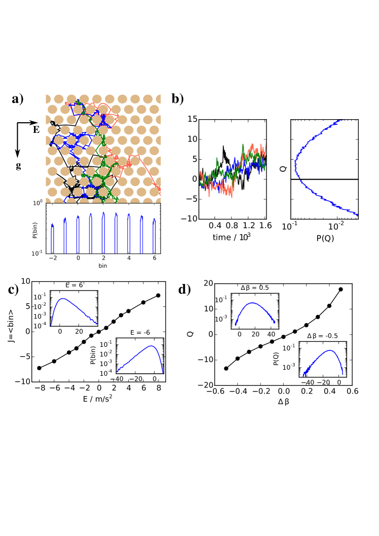
Figure 1: Tracking the horizontal flow through the Galton board setup (left panels) or the heat flux from mode 7 to mode 3 in the Fermi-Pasta-Ulam lattice (right panels). Example trajectories, along with a histogram of total flux at a single applied force are shown in a,b, while c,d summarize all simulations by showing the average flux as a function of applied force. The insets of c,d show histograms of the flux at large values of the force.

Figure 1a shows four randomly chosen trajectories for the system, along with the complete histogram collected at row 10 for a small positive value of $E$. The flux, $J$, is identical to the final bin number, determined from the $x$-coordinate. The results presented here were collected from the hexagonal lattice shown with particle-to-scatter contact distance of 0.4$L$. The time scale, $\tau$, was set so that the gravitation constant is $9.8m/s^{2}=1L/\tau^{2}$. 102,400 trajectories were simulated with uniform random starting locations on the line $y=0,x\in(-0.1L,0.1L)$ and velocities chosen from a Gaussian distribution with variance $(\beta M)^{-1}=5.292\cdot 10^{-19}~{}\tau^{2}/L^{2}$. This is consistent with a physical scatterer diameter of 6.35 cm and mass of 5 g. Complete details are in the appendix.

This type of model (under constant field) has been applied to study electron motion through insulators.achep01 The zero-forcing case with elastic scattering was studied analytically by Sinai,jlebo73 ; lbumo81 who showed that the trajectory of the particle over long times converges to a Brownian random walk, and that the expected direction of motion remains constant over time. The evolution of the probability density can be shown to converge to a Boltzmann transport equation,ggall69 ; cbold83 and even has intuitive diffusive properties under a small, constant external force.ncher08 A review of approaches to the Lorentz gas was given by Spohn.hspoh80 In the real-world case, the parabolic trajectories followed by the particle make exact analysis difficult. An analysis using a constant kinetic energy thermostat showed strong chaotic properties, including fractal scaling of the probability distributions for particle-scatterer impact.whoov89 With elastic collisions, the kinetic energy of the particle must increase linearly as the particle falls. For this case, it has recently been shown that the particle velocity grows with time as $t^{1/3}$, and that (analogous to the Gambler’s ruin problem) for large enough starting velocity the particle will return to its initial height with probability 1.ncher09 Our setup differs from these earlier studies because of the presence of constant external force, inelastic collisions, and angular velocity.

III.2 Mode-Coupled Fermi-Pasta-Ulam Chains

To examine the time-course of energy redistribution between harmonic modes of a crystal lattice, Fermi, Pasta, and Ulam (FPU) simulated 32 points moving in 1D with unit masses and coordinates,tdaux05 $x_{j},j=1,\ldots,N$. This work uses periodic boundaries, so $x_{0}=x_{N}$. The potential energy function is,

$$U(x) =\sum_{j=0}^{N-1}V(x_{j+1}-x_{j})$$ (20)

$$V(r) =r^{2}/2+\alpha r^{3}/3.$$ (21)

They discovered that for small anharmonic terms, energy did not seem to exchange, but only to oscillate regularly between harmonic modes. Recent, much longer, simulations and theory have shown that systems with small $\alpha$ do, in fact, equilibrate but on an enormously long time-scale on the order of $\alpha^{-8}$.monor15 This phenomenon has been explained as due to the nearness of $V(r)$ with the potential for the Toda lattice, $e^{r}-r-1$, which is exactly integrable.

To simulate this system numerically, we began by deriving a symplectic, volume-preserving dynamical integration scheme based on the Lagrangian,

$$L(x,\dot{x})=\sum_{j}\frac{\dot{x}_{j}^{2}}{2}-V(x).$$ (22)

Following the procedure of Marsden,jmars01 we make the substitutions, $\dot{x}\to(x^{(t)}-x^{(t-1)})/\Delta t$, $x\to x^{(t)}$, to construct a discrete action functional,

$$A[\{x\}] =\sum_{t=1}^{T}L_{d}(x^{(t)},x^{(t-1)})$$ (23)

$$L_{d}(x^{\prime},x) =\sum_{j}\frac{(x^{\prime}_{j}-x_{j})^{2}}{2\Delta t}-\Delta tV(x^{\prime}).$$ (24)

Requiring stationary action yields,

$$\frac{\partial L_{d}(x^{\prime},x)}{\partial x^{\prime}}+\frac{\partial L_{d}(x^{\prime\prime},x^{\prime})}{\partial x^{\prime}}=0,$$ (25)

which translates to the Strömer-Verlet scheme,

$$\frac{x^{\prime\prime}-x^{\prime}}{\Delta t}+\frac{x-x^{\prime}}{\Delta t}+\Delta t\frac{\partial V(x^{\prime})}{\partial x^{\prime}}=0.$$ (26)

Rather than adding a thermostat to the coordinate-space integrator of Eq. 26, we chose to cast the time integration in Fourier space,

$$X_{k}=\sum_{j=1}^{N}u^{-jk}x_{j},\quad u\equiv e^{2\pi i/N},\quad\omega_{k}^{2}\equiv|u^{k}-1|^{2}.$$ (27)

The versatility of the Lagrangian approach is exploited by re-writing Eq. 24 in these new coordinates ($P_{k}\equiv(X_{k}^{\prime}-X_{k})/\Delta t$),

$$L_{d}(X^{\prime},X) =\frac{\Delta t}{2N}\sum_{k=0}^{N-1}\left[|P_{k}|^{2}-\omega_{k}^{2}|X_{k}^{\prime}|^{2}\right]-\Delta tV_{c}(X^{\prime}).$$ (28)

Here, $V_{c}$ represents the cubic potential terms. According to MaxTrans, the exponent of the transition probability should be,

$$-\frac{\Delta t}{2\sigma^{2}}\left|\frac{\delta A[X(t)]}{\delta X(t)}\right|^{2}+\frac{\beta}{2}dX(t)\cdot\frac{\delta A[X(t)]}{\delta X(t)}.$$ (29)

Note how Eq. 6 behaves under a change in coordinate systems. It simply amounts to transforming the deviations, $\sigma$, via the Jacobian, $|dx/dX|$. The thermostatted equations of motion for $X_{k}$ can be read off from the mean and variance found by factoring Eq. 29

$$-\left(\frac{\delta A[X_{k}(t)]}{\delta X_{k}(t)}\right)^{*}\Delta t=-\frac{\beta_{k}\sigma_{k}^{2}}{2}dX_{k}(t)+\sigma_{k}d\mathcal{W}_{k}.$$ (30)

This equation of motion must be interpreted as applying to only $N$ degrees of freedom. Since $X_{k}=X_{-k}^{*}$, the unique discrete Fourier variables are Re[$X_{0},X_{1},\ldots,X_{\lceil(N-1)/2\rceil}$] and Im[$X_{1},\ldots,X_{\lfloor(N-1)/2\rfloor}$].

Energy exchange processes can be monitored by examining various decompositions of the energy change (right side of Eq. 29),

$$dE=dX^{*}\left(\frac{dP}{dt}-F_{\text{harm}}-F_{\text{cubic}}\right).$$ (31)

By decomposing the total force as $dP/dt=F_{\text{harm}}+F_{\text{cubic}}+F_{\text{lang}}$, we get

$$dE=dX^{*}F_{\text{lang}}=dX^{*}\left(\frac{dP}{dt}-F_{\text{harm}}\right)-dX^{*}F_{\text{cubic}}\\ .$$ (32)

Of course, the first term on the right side just integrates to the sum of energies in the unperturbed harmonic modes, $E_{k}(t)-E_{k}(0)$, where

$$E_{k}+E_{-k}=(|P_{k}|^{2}+\omega_{k}^{2}|X_{k}|^{2})/2N.$$ (33)

We could separate the $\pm k$ parts by choosing a phase arbitrarily. From this point of view, the time-derivative of $E_{k}$ (the energy in each mode), represents the flux of energy from both the anharmonic system and the Langevin thermostat.

To filter out noise coming from the Langevin thermostat, we define the ‘heat flux’ into mode $k$ to be the integral of the second term, $dQ_{k}=dX^{*}F_{\text{cubic}}$. It was computed numerically as the difference between the harmonic oscillator’s energy change and the energy added from the Langevin thermostat. Comparing to Eq. 33 shows $E_{k}(t)-E_{k}(0)=Q_{k}+Q_{k}^{\text{Langevin}}$. All heat flows, $Q$, thus come directly from energy exchange through anharmonicity. For individual modes that are coupled to a ‘hot’ reservoir, we will accordingly observe heat flow out of that mode into anharmonic degrees of freedom. No heat flow between modes is possible when $\alpha=0$. This was verified numerically to test our implementation.

Fig. 1b shows example trajectories of energy flow from mode $k=7$ to $k=3$ in the FPU system at $\alpha=0.1$. To provide a steady-state with energy flow, both modes $k=\pm 3$ and $k=\pm 7$ were coupled to Langevin thermostats with $\beta_{3}=1+\Delta\beta$ and $\beta_{7}=1-\Delta\beta$, respectively, and $\sigma_{3}=\sigma_{7}=0.1$. All other modes remained un-thermostatted (equivalent to setting $\sigma^{2}_{k}=0$).

Distributions of $Q=Q_{3}-Q_{7}$ presented here were calculated at time 1638.4 from a Verlet integration scheme with timestep $0.01$. They include an initial transient of approximately 100 time units because the initial conditions were chosen from the canonical distribution for the harmonic system ($\alpha=0$) at uniform temperature $\beta=1$.

Fig. 1c,d shows that the flow is a nonlinear function of the applied force ($\vec{E}$ for the Lorentz gas or $\Delta\beta$ for the FPU lattice). This is especially apparent at large values of the forcing, where the probability distributions over flow ($J$ for the Lorentz gas or $Q$ for the FPU lattice) are markedly non-Gaussian. These flows are totals, integrated over the first 10 rows for the Lorentz system or the first 1638.4 time units for the FPU system. Because of this they include part of the initial transient as it relaxes to a conducting steady-state.

IV Discussion and Comparison

Often, applied literature provides specialized fluctuation-dissipation or fluctuation theorems that give little hint as to how they may be generalized or extended. In fact, the original derivations allow quite a bit of flexibility in defining what forces and flows can enter, and can be put into a form very much resembling our major results (Eqns. 8, 9, and 10). We discuss these alternative viewpoints by standardizing the notation and re-stating the theorems in terms of time-derivatives (flows) rather than absolute positions.

IV.1 Projector-Operator and Fluctuation-Dissipation Theorems

The projector-operator theory gives a rigorous, general equation of motion for the probability distribution of coarse coordinates like the particle position or the energy in each mode. The theory clearly indicates where closure relations are required. This section shows how the simplest closure relations with Gaussian noise can be derived by analogy to Gaussian processes. The result provides time-dependent Green-Kubo relations applicable at nonzero driving force. They are linear because they predict only the slope of the flow vs. force curve.droge11a

An accessible derivation of the projector-operator theory was given by Nordholm and Zwanzigsnord75 with the result,

$$\frac{\partial}{\partial t}\mathbb{P}f(t,\Gamma)=-\mathbb{P}i\mathcal{L}\mathbb{P}f(t,\Gamma)$$

$$+\int_{0}^{t}\;ds\mathbb{P}i\mathcal{L}e^{-is(1-\mathbb{P})\mathcal{L}}(1-\mathbb{P})i\mathcal{L}\mathbb{P}f(t-s,\Gamma)$$

$$-\mathbb{P}i\mathcal{L}e^{-it(1-\mathbb{P})\mathcal{L}}(1-\mathbb{P})f(0,\Gamma).$$ (34)

The operator, $\mathbb{P}$, projects the phase-space probability density, $f(t,\Gamma)$, onto a subspace of the full phase space, $\Omega=\{\Gamma\}$. The Liouville operator is defined in terms of the Poisson brackets, $i\mathcal{L}J=\{J,H\}=dJ/dt$. There is no difficulty interpreting this subspace as an arbitrary manifold lying inside $\Omega$. For any point, $\Gamma$, we can define the projected point on the manifold as $\phi(\Gamma)$ so that

$$\mathbb{P}f(\Gamma)=\int_{\Omega}d\Gamma^{\prime}\;\delta(\Gamma-\phi(\Gamma^{\prime}))f(\Gamma^{\prime}).$$ (35)

The projected equation of motion (Eq. 34) implicitly defines the probability distribution of transition events, $g=\phi(\Gamma)\to\phi(\Gamma^{\prime})$. It is trivial to re-cast it in this way, since $dt\frac{\partial}{\partial t}\mathbb{P}f(t,\Gamma)=\int dg\;\operatorname{P}\left(\Gamma|\Gamma^{\prime},dt\right)f(t^{\prime},\Gamma^{\prime})-f(t^{\prime},\Gamma)$ as the timestep, $dt\to 0$.

The push-forward operation, $i\mathcal{L}\mathbb{P}f(t,\Gamma)$, in both of the first two terms refers explicitly to this transition. The three parts of the equation of motion on the manifold (Eq. 34) have the interpretation of i) the deterministic transition ($\mathbb{P}i\mathcal{L}\mathbb{P}$) for points on the manifold, ii) the memory function describing the predictable, but delayed effect due to earlier transitions, $(1-\mathbb{P})i\mathcal{L}\mathbb{P}f(t-s,\Gamma)$, and iii) the ‘random’ noise part due to initial conditions not on the manifold.

Because they are off the manifold, the equation of motion makes it clear that closure relations are required for describing parts (ii) and (iii). Specific choices for those closures form the starting points for mode coupling theorysnord75 and nonlinear fluctuating hydrodynamics.gmaze06 That theory has also been applied to dynamics in large-FPU chains.cmend13

In practice, most applications of the theory have used linear closure relations, which give rise to linear transport equations.rzwan65 Nonlinear closures are most easily understood by comparison to the linear theory.rkubo66 It has been pointed outejayn80 that the principle results of the linear theory are identical to linear regression.

The linear regression case has been treated in a very general way in the Gaussian process literature. The critical assumptions are that the random noise obeys Gaussian statistics and that the coefficients of the memory function depend only on time, not on the process history. The equations below relate to the two systems considered here by replacing $g$ with the horizontal motion of the disk, $dJ$, or the heat transfer, $dQ$, over a small amount of time. The regression equations can be summarized by the assumption,crasm06

$$\operatorname{P}\left(\{g(t_{i})\}_{0}^{n}\right)=GP[m(t_{i}),k(t_{i},t_{j})]$$ (36)

which implies the following generating process,

$$g(t_{n}) =m(t_{n})+\sum_{j,k=1}^{n}k(t_{n},t_{n-j})k^{-1}_{n-j;n-k}$$

$$\times(g(t_{n-k})-m(t_{n-k}))+\sigma_{n}R_{n}$$ (37)

$$\sigma^{2}_{n}=k(t_{n},t_{n})-\sum_{j,k=1}^{n}k(t_{n},t_{n-j})k^{-1}_{n-j;n-k}k(t_{n},t_{n-k})$$ (38)

Here, $GP$ denotes a Gaussian process, which is a multivariate normal distribution with mean $m(t)$ and variance-covariance matrix $k(t,t^{\prime})$. Eq. 37 states the applicable fluctuation-dissipation theorem – namely that the probability of $g$ at the next step has a Gaussian distribution with a mean that is linear in the random increments, $g(t_{k})-m(t_{k})$, and a variance, $\sigma_{n}^{2}$, that is reduced by knowledge of the process history. The variable $R_{n}$ is an independent sample from the standard normal distribution.

This closure is demonstrated by noting the terms in Eq. 37 correspond 1:1 with those of Eq. 34. Brownian motion theory is recovered when $g$ is taken to be the momentum. Then $m(t)$ is the drift velocity and $k(t,t)=k_{B}T/m$ near equilibrium. Its time-derivative describes Langevin dynamics, where $g_{n}$ is the momentum update, $p_{n}-p_{n-1}$.

From these identifications, a little algebra shows that applying a single external force at time $t_{0}$ will not only directly shift $g_{0}\to g_{0}+F^{\text{ext}}_{0}$, but will also accumulate a net effect at later times, $t_{k}$ of,

$$\delta g_{k\leftarrow 0} =\begin{bmatrix}k(t_{k},t_{I})\end{bmatrix}^{T}k^{-1}_{IJ}\begin{bmatrix}\delta g_{0}\\ \delta g_{1\leftarrow 0}\\ \vdots\\ g_{k-1\leftarrow 0}\end{bmatrix}$$ (39)

The recursion is solved by

$$\delta g_{k\leftarrow 0} =\frac{k(t_{k},t_{0})}{k(t_{0},t_{0})}F^{\text{ext}}_{0}.$$ (40)

In comparison with our main result (Eq. 8), this externally forced process could have been derived extremely easily by adding an exponential bias to the basic Gaussian process (Eq. 36),

$$\operatorname{P}\left(\vec{g}|F^{\text{ext}}\right)\propto\exp\Big{\{} -(\vec{g}-\vec{m})^{T}k^{-1}(\vec{g}-\vec{m})/2$$

$$+(\vec{g}-\vec{m})^{T}(F^{\text{ext}}/\mathrm{diag}(k))\Big{\}}.$$ (41)

This is the revised Onsager-Machlup action functional approach.lonsa53 ; lbert15

The linear transport theory can be re-derived in a simplified way as a Gaussian process. The technical content of the celebrated fluctuation-dissipation theorem in this case is a statement of how dissipation of an external force, $\sum_{j<n}k(t_{n},t_{n-j})$, is related to fluctuations of the current, $k(t_{i},t_{j})=\left\langle\delta g_{i}\delta g_{j}\right\rangle$.

We can see that this line of attack applies to time-dependent processes, but Gaussian processes do not make it clear how to extend the theory into the nonlinear regime. The major contribution of Sec. II was to replace the fitting ansatz of Eq. 36 with a single-step fitting ansatz at time $t_{i}$. This frees $m_{i}$ and $k_{ij}$ to be arbitrary nonlinear functions of the history, $\{g\}_{0}^{i-1}$. However, it sacrifices knowledge of the steady-state properties.

IV.2 Fluctuation Theorems and Chaotic Hypothesis

Fluctuation theorems address the probabilities of transitions even more directly. Specifically, they transform symmetries of the dynamical equations into symmetries of integrated quantities such as work and heat. They have a history stretching back to Callen and Welton,hcall52 who proved a fluctuation theorem showing the odds of heat, $Q$, flowing from cold to hot vs. the reverse process was proportional to $\exp(Q\Delta\beta)$.

Since the literature on fluctuation theorems is large, I provide here only a few results. The first fluctuation theorems about atomistic trajectories were developed by several groups,devan02 ; ggall08 who proved theorems of the form,

$$\frac{1}{t}\log\frac{\operatorname{P}\left(g=\sigma(t,\Gamma)/t|x_{0}\to x_{n}\right)}{\operatorname{P}\left(g=-\sigma(t,\Gamma)/t|x_{n}\to x_{0}\right)}\asymp g$$ (42)

The symbol, $\asymp$, means asymptotic convergence with large time, $t$. The conditioning on coordinates, $x_{0}$ or $x_{n}$, indicates whether the trajectory is initiated from a starting or ending point. For the transient fluctuation theorem, the microscopic entropy production is identified with the time-integral over a trajectory of length $t$ starting from $\Gamma(0)=\Gamma$,

$$\sigma(t,\Gamma)=\int_{0}^{t}dt\;D(\Gamma(t)),$$ (43)

where $D(\Gamma)$ is the ratio of phase space volume between the last and next time-step, $|i\mathcal{L}(d\Gamma)|/|d\Gamma|$. Because of the dependence on the starting/ending point, there are differences in the relations and proofs depending on whether the starting states are fixed or chosen at random from an SRB measure (steady-state), whose existence and uniqueness requires additional assumptions.ggall96

In the case where a dynamical system can be modeled as a finite-state Markov process, a new version of the fluctuation theorem (Eq. 42) can be shown,jlebo99 ; gcroo00 where $\sigma$ ($W$ of Ref. 43) is the log-ratio of forward to reverse transition probabilities over $t=n$ steps of the Markov process,

$$\sigma(n,\Gamma)=\sum_{i=0}^{n-1}\log\frac{\operatorname{P}\left(\Gamma_{i+1}|\Gamma_{i}\right)}{\operatorname{P}\left(\Gamma_{i}|\Gamma_{i+1}\right)}.$$ (44)

Although they apply in different cases, the two fluctuation relations essentially express the same measure of irreversibility, since the probability of a transition scales inversely with the starting volume, $\operatorname{P}\left(\Gamma_{i+1}|\Gamma_{i}\right)\propto 1/|d\Gamma_{i}|$.

Since the log-ratio of transition probabilities are often related to work and entropy production, the fluctuation theorems can make quantitative statements about energy exchange during transitions of a dynamical system. Although Eq. 42 appears to be a special case of Eq. 10, Eq. 42 has been proven to hold under more general conditions. Its relation to symmetry provides it with a unique status in that it is closer to a dynamical law than a statistical one.

It is also possible to specialize $\sigma$ for describing transition probabilities of other coarse variables.devan02 ; ggall95 This interpretation often refers to $\sigma$ as a dissipation function, or, in reference to the Onsager-Machlup theory, as an action function. Our alternative derivation of $\sigma$ as a generalized entropy in section II provides a more canonical explanation of this connection between $\sigma$ and force/flux relations.

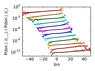
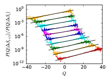
Figure 2: Log-probability ratios for successive values of the applied force. Forces increase left-to-right, with each line shifted down by a factor of 10 for visual separation. Black lines show linear fits to these log-ratios. The left panel shows data from the Galton board, while the right shows heat conduction in the FPU lattice.

Postulates like Eq. 3 have been hinted at before in connection with Onsager-Machlup theoryhfors08 , but their generality and use for deriving fluctuation theorems has not been widely appreciated. A similar theory of Jaynes, named maximum caliber (MaxCal),ejayn80 applied maximum entropy to the set of all trajectories. Unfortunately, that theory does not maintain causality,droge12 since forces applied in the future influence the entire history of the process. This shortcoming has not caused identifiable problems where the theory has been applied,gstoc08 ; spres11 ; kdill15 since maximum caliber and MaxTrans make the same probability assignments when there is time translation invariance of the forces. In these situations, non-causality only creates problems when applying the fluctuation theorems. The situation can be summed up by noting that path counting gives non-causal weights to trajectories, whereas the transition probabilities are always causal.

Both Jaynesejayn85 and Hakenhhake85 ; hhake93 investigated maximizing the entropy of the transition distribution as a restriction of MaxCal. Those early works chose steady-state averages as constraints, rather than the instantaneous flows as done here. Since the Lagrange multipliers had to be identified through the Fokker-Planck equation, that choice hid the connection to the equilibrium, Boltzmann/Gibbs distribution. Had they made the latter choice, they would have immediately discovered our kinetic partition function, $\mathcal{Z}_{\text{kin}}$, along with its attendant force-flux relationships and FDTs.

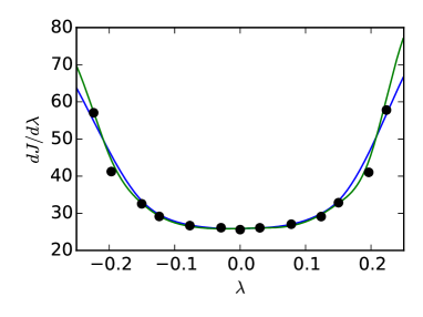
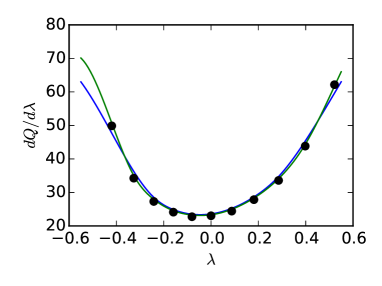
Figure 3: Comparison between asymptotically equivalent expressions for the conductivity coefficient. The lines show different numerical estimates of derivatives of the flux vs. force curves ($d\left\langle J\right\rangle/d\lambda$) computed from alternate finite difference methods, while the variance of the flux ($\left\langle\delta J^{2}|\lambda\right\rangle$) is shown as individual points. The blue line uses a 3${}^{\text{rd}}$ order finite difference interpolation of $J(\lambda)$ (Fig. 1c,d) and the green line uses a 7${}^{\text{th}}$ order interpolation from the same data. The left panel shows data from the Galton board, while the right shows heat conduction in the FPU lattice.

Figure 3 compares properties i and ii (listed at the end of Sec. II) by plotting $d\left\langle J|\lambda\right\rangle/d\lambda$ (lines) from the force-flux curves of Fig. 1 against the fluctuations $\left\langle\delta J^{2}\right\rangle_{\lambda}$ (shown as points). The two smooth lines on each plot come from the derivatives obtained from 3${}^{\text{rd}}$ and 7${}^{\text{th}}$ order numerical differencing schemes. Differences between these lines are a measure of the uncertainty in collected force vs. flux data. The correspondence, $\lambda=\lambda(E)$ or $\lambda(\Delta\beta)$, was made by the fits to the slopes in Fig. 2. Linear response predicts that $\left\langle J\right\rangle$ will be proportional to $\lambda$, $\lambda$ proportional to the force, and hence $\left\langle\delta J^{2}\right\rangle$ will be constant. While $\left\langle\delta J^{2}\right\rangle$ is almost constant near the origin for the Lorentz gas, linear response clearly does not hold in the FPU system. Nevertheless, our numerical data show the validity of Eq. 10 well out of the linear response regime. Fig. 2 shows method i and Fig. 3 shows method ii. The fluctuations of the current still correspond to the slope of the flux-force curve away from the region of “constant” $\left\langle\delta J^{2}\right\rangle$ around $\lambda=0$.

The canonical form of Eq. 7 codifies flux/force relations in a coordinate-independent way using a maximum entropy structure. Because of this, it provides facile derivations for both time-dependent Green-Kubo response theories and the fluctuation theorems when the postulate of Eq. 3 holds. Its shortcoming is that it does not directly predict the relationship between the forces and flows, e.g. $\beta$ and $\left\langle dE\right\rangle$. This, however, is exactly the well-known problem of determining the equations of state in equilibrium statistical mechanics.

V Conclusions

We have constructed a probability distribution over values of flows that occur during transitions using maximum entropy. It was shown that the nonlinear, maximum entropy structure is a general consequence of an unknown, and hence subjectively random, environment. For atomistic problems, a general prescription exists to derive a generalized Langevin equation from an action functional. For coarse-grained properties, Eq. 3 just states the maximum entropy postulate and must be experimentally verified wherever it is used. Numerical simulationsof driven diffusion in 2D gas models and heat diffusion between modes of a crystal supported it. We expect the postulate to be more easily satisfied as the number of transitions grows – even for transient, driven processes. The success of the linear response methods and of the fluctuation theorems both rest on exploiting the existence of this structure within the transition distribution.

This theory has been directly related to two complementary methods of attack. The Green-Kubo relations provide quick estimates for the conductivities, even in transient steady-states. This work showed the connection by focusing on the transition quantities in Eq. 37, which have the same structure as Eq. 8 and 9. Fluctuation theorems provide connections with distributions of work and notions of irreversibility. We have shown the forward fluctuation relation of Eq. 10 derives Eq. 42 when the flux is related to number of transitions. Transition distributions provide an entry point to these theories, but can also be applied in their own right as a maximum entropy structure. Although it derives mathematically identical results, it is logically distinct from large deviation theories because maximum entropy infers transition distributions even when the underlying microscopic noise process is unknown. It is also distinct from Gaussian processes or near-equilibrium theories that use the idea of local entropies because it focuses specifically on one-step transitions.lonsa53 ; iprig65 ; hspoh78 ; ejayn80 All general approaches are structural in the sense that finding analytical expressions for long-time force/flux relationships is a difficult task, even for for the Lorentz gasachep01 ; ncher08 and FPU heat models.jeckm99 ; hspoh14 ; monor15 Our line of reasoning avoids that problem, and instead parallels the reasoning used to derive equilibrium equations of state. Its most common criticism – that certain analytic properties of the microscopic distribution must be proven – directly parallels the integrability objection to the ergodic hypothesis.

References

- [1] Carlos Bustamante, Jan Liphardt, and Felix Ritort. The nonequilibrium thermodynamics of small systems. Phys. Today, 58(7):43–48, 2005.
- [2] Christian Maes, Karel Netočný, and Bram Wynants. Steady state statistics of driven diffusions. Physica A, 387(12):2675–2689, 2008.
- [3] C. Jarzynski. Diverse pheonomena, common themes. Nature Phys., 11:105–107, 2015.
- [4] Raphaël Chetrite and Hugo Touchette. Nonequilibrium Markov processes conditioned on large deviations. Ann. Henri Poincaré, 16(9):2005–2057, 2015.
- [5] S. R. S. Varadhan. Large deviations. Ann. Prob., 36(2):397–419, 2008.
- [6] F. Bonetto, G. Gallavotti, and P. L. Garrido. Chaotic principle: An experimental test. Physica D, 105:226–252, 1997.
- [7] Hugo Touchette. The large deviation approach to statistical mechanics. Phys. Rep., 478(1–3):1–69, 2009.
- [8] David M Rogers and Susan B Rempe. Irreversible thermodynamics. J. Phys., Conf. Ser., 402:012014, 2012.
- [9] E. T. Jaynes. Information theory and statistical mechanics. Phys. Rev., 106(4):620–630, May 1957.
- [10] Joel Lebowitz and Oliver Penrose. Modern ergodic theory. Physics Today, 26(2):23–29, 1973.
- [11] E. T. Jaynes. Where do we stand on maximum entropy? In R. D. Levine and M. Tribus, editors, The Maximum Entropy Formalism, page 498. M.I.T Press, Cambridge, 1979.
- [12] Christian Maes. The fluctuation theorem as a gibbs property. J. Stat. Phys., 95(1/2):367–392, 1999.
- [13] David M. Rogers, Thomas L. Beck, and Susan B. Rempe. An information theory approach to nonlinear, nonequilibrium thermodynamics. J. Stat. Phys., 145(2):385–409, 2011.
- [14] Da-Quan Jiang, Min Qian, and Fu-Xi Zhang. Entropy production fluctuations of finite Markov chains. J. Math. Phys., 44(9):4176, 2003.
- [15] Lamberto Rondoni and Carlos Mejía-Monasterio. Fluctuations in nonequilibrium statistical mechanics: models, mathematical theory, physical mechanisms. Nonlinearity, 20(10):R1, 2007.
- [16] Lorenzo Bertini, Alberto De Sole, Davide Gabrielli, Giovanni Jona-Lasinio, and Claudio Landim. Macroscopic fluctuation theory. Rev. Mod. Phys., 87:593–636, Jun 2015.
- [17] Giovanni Gallavotti. Extension of Onsager’s reciprocity to large fields and the chaotic hypothesis. Phys. Rev. Lett., 77:4334–4337, Nov 1996.
- [18] David M. Rogers. An information theory model for dissipation in open quantum systems. J. Phys. Conf. Series, 880(1):012039, 2017. 8th International Workshop DICE2016.
- [19] S. Gao, editor. How to Teach and Think About Spontaneous Wave Function Collapse Theories: Not Like Before, pages 3–11. Cambridge Univ. Press, Cambridge UK, 2018.
- [20] Denis J. Evans, Debra J. Searles, and Stephen R. Williams. Fundamentals of Classical Statistical Thermodynamics. Wiley, 2016.
- [21] A. D. Chepelianskii and D. L. Shepelyansky. Dynamical turbulent flow on the Galton board with friction. Phys. Rev. Lett., 87:034101, Jun 2001.
- [22] L. A. Bunimovich and Y. G. Sinai. Statistical properties of Lorentz gas with periodic configuration of scatterers. Commun. Math. Phys., 78:479–497, 1981.
- [23] G. Gallavotti. Divergences and the approach to equilibrium in the Lorentz and the wind-tree models. Phys. Rev., 185:308, 1969.
- [24] C. Boldrighini, L. A. Bunimovich, and Ya. G. Sinai. On the Boltzmann equation for the Lorentz gas. J. Stat. Phys., 32(3):477–501, 1983.
- [25] N. Chernov. Sinai billiards under small external forces II. Ann. Henri Poincaré, 9(1):91–107, 2008.
- [26] H. Spohn. Kinetic equations from Hamiltonian dynamics: Markovian limits. Rev. Mod. Phys., 52(3):569–615, 1980.
- [27] W. G. Hoover and B. Moran. Phase-space singularities in atomistic planar diffusive flow. Phys. Rev. A, 40(9):5319–5326, 1989.
- [28] N. Chernov and D. Dolgopyat. The Galton board: Limit theorems and recurrence. J. Amer. Math. Soc., 22:821–858, 2009.
- [29] Thierry Dauxois, Michel Peyrard, and Stefano Ruffo. The Fermi-Pasta-Ulam “numerical experiment”: history and pedagogical perspectives. Eur. J. Phys., 26(5):S3, 2005.
- [30] M. Onorato, L. Vozella, D. Proment, and Y. V. Lvov. Route to thermalization in the -Fermi-Pasta-Ulam system. Proc. Nat. Acad. Sci. USA, 112(14):4208–4213, 2015.
- [31] J. E. Marsden and M. West. Discrete mechanics and variational integrators. Acta Numerica, 10:357–514, 2001.
- [32] Sture Nordholm and Robert Zwanzig. A systematic derivation of exact generalized Brownian motion theory. J. Stat. Phys., 13(4):347–371, 1975.
- [33] Gene F. Mazenko. Nonequilibrium Statistical Mechanics. Wiley-VCH, 2006.
- [34] Christian B. Mendl and Herbert Spohn. Dynamic correlators of fermi-pasta-ulam chains and nonlinear fluctuating hydrodynamics. Phys. Rev. Lett., 111:230601, 2013.
- [35] R. Zwanzig. Time-correlation functions and transport coefficients in statistical mechanics. Ann. Rev. Phys. Chem., 16:67–102, 1965.
- [36] R. Kubo. The fluctuation-dissipation theorem. Rep. Prog. Phys., 29:255, 1966.
- [37] E. T. Jaynes. The minimum entropy production principle. Ann. Rev. Phys. Chem., 31:579–601, 1980.
- [38] Carl Edward Rasmussen and Christopher K. I. Williams. Gaussian Processes for Machine Learning. MIT Press, 2006.
- [39] L. Onsager and S. Machlup. Fluctuations and irreversible processes. Phys. Rev., 91(6):1505–1512, Sep 1953.
- [40] Herbert B. Callen and Richard F. Greene. On a theorem of irreversible thermodynamics. Phys. Rev., 86(5):702–710, Jun 1952.
- [41] Denis J. Evans and Debra J. Searles. The fluctuation theorem. Advances in Phys., 51(7):1529–85, 2002.
- [42] G. Gallavotti. Heat and fluctuations from order to chaos. Eur. Phys. J. B, 61:1–24, 2008.
- [43] Joel L. Lebowitz and Herbert Spohn. A Gallavotti–Cohen-type symmetry in the large deviation functional for stochastic dynamics. J. Stat. Phys., 95:333–365, 1999.
- [44] Gavin E. Crooks. Path-ensemble averages in systems driven far from equilibrium. Phys. Rev. E, 61(3):2361–2366, Mar 2000.
- [45] To make this statement rigorous requires comparing the number of transitions that can be made out of state vs. those out of state .
- [46] G. Gallavotti and E. G. D. Cohen. Dynamical ensembles in nonequilibrium statistical mechanics. Phys. Rev. Lett., 74(14):2694–2697, 1995.
- [47] H. Förster and M. Büttiker. Fluctuation relations without microreversibility in nonlinear transport. Phys. Rev. Lett., 101:136805, Sep 2008.
- [48] Gerhard Stock, Kingshuk Ghosh, and Ken A. Dill. Maximum caliber: A variational approach applied to two-state dynamics. J. Chem. Phys., 128(19):194102, 2008.
- [49] S. Press, K. Ghosh, and K. A. Dill. Modeling stochastic dynamics in biochemical systems with feedback using maximum caliber. J. Phys. Chem. B, 115(19):6202–6212, 2011.
- [50] Michael J. Hazoglou, Valentin Walther, Purushottam D. Dixit, and Ken A. Dill. Communication: Maximum caliber is a general variational principle for nonequilibrium statistical mechanics. J. Chem. Phys., 143(5):051104, 2015.
- [51] E. T. Jaynes. Macroscopic prediction. In H. Haken, editor, Complex Systems - Operational Approaches in neurobiology, pages 254–269, 1985.
- [52] Hermann Haken. Application of the Maximum (Information) Entropy Principle to Stochastic Processes far from Thermal Equilibrium, volume 119 of Studies in Fuzziness and Soft Computing, pages 79–89. Springer, 1985.
- [53] H. Haken. Application of the Maximum Entropy Principle to Nonlinear Systems Far From Equilibrium, pages 239–250. Cambridge Univ. Press, 1993.
- [54] I. Prigogine. Steady states and entropy production. Physica, 31(5):719–724, 1965.
- [55] Herbert Spohn and Joel L. Lebowitz. Irreversible thermodynamics for quantum systems weakly coupled to thermal reservoirs. In Stuart A. Rice, editor, Adv. Chem. Phys., volume 38, pages 109–142. Wiley, 1978.
- [56] J. P. Eckmann, C. A. Pillet, and L. Rey-Bellet. Non-equilibrium statistical mechanics of anharmonic chains coupled to two heat baths at different temperatures. Commun. Math. Phys., 201:657–697, 1999.
- [57] H. Spohn. Nonlinear fluctuating hydrodynamics for anharmonic chains. J. Stat. Phys., 154(5):1191–1227, 2014.
- [58] TitlesOn. Titleson. TitlesOn, TitlesOn, 1900.