Magneto-static modelling from Sunrise/IMaX: Application to an active region observed with Sunrise II.

Abstract

Magneto-static models may overcome some of the issues facing force-free magnetic field extrapolations. So far they have seen limited use and have faced problems when applied to quiet-Sun data. Here we present a first application to an active region. We use solar vector magnetic field measurements gathered by the IMaX polarimeter during the flight of the Sunrise balloon-borne solar observatory in June 2013 as boundary condition for a magneto-static model of the higher solar atmosphere above an active region. The IMaX data are embedded in active region vector magnetograms observed with SDO/HMI. This work continues our magneto-static extrapolation approach, which has been applied earlier (Paper I) to a quiet Sun region observed with Sunrise I. In an active region the signal-to-noise-ratio in the measured Stokes parameters is considerably higher than in the quiet Sun and consequently the IMaX measurements of the horizontal photospheric magnetic field allow us to specify the free parameters of the model in a special class of linear magneto-static equilibria. The high spatial resolution of IMaX (110-130 km, pixel size 40 km) enables us to model the non-force-free layer between the photosphere and the mid chromosphere vertically by about 50 grid points. In our approach we can incorporate some aspects of the mixed beta layer of photosphere and chromosphere, e.g., taking a finite Lorentz force into account, which was not possible with lower resolution photospheric measurements in the past. The linear model does not, however, permit to model intrinsic nonlinear structures like strongly localized electric currents.

1 Introduction

Getting insights into the structure of the upper solar atmosphere is a challenging problem, which is addressed observationally and by modelling (Wiegelmann et al., 2014). A popular choice for modelling the coronal magnetic field are so called force-free configurations (see Wiegelmann & Sakurai, 2012, for a review), because of the low plasma $\beta$ in the solar corona above active regions, (see Gary, 2001). A complication with this approach is that necessary boundary conditions for force-free modelling, namely the vector magnetograms, are routinely observed mainly in the solar photosphere, where the force-free assumption is unlikely to be valid (see, e.g., DeRosa et al., 2009, 2015, for consequences on force-free models.).

A principal way to deal with this problem is to take non-magnetic forces into account in the lower solar atmosphere (photosphere to mid chromosphere) and to use force-free models only above a certain height, say about 2 Mm, where the plasma $\beta$ is sufficiently low. Due to the insufficient spatial resolution of vector magnetograms in the past (e.g. pixel size about 350 km for SDO/HMI, which corresponds to a resolution of 700 km), trying to include the relatively narrow lower non-force-free layer in a meaningful way was questionable. Nevertheless even with the low resolution of SOHO/MDI magnetograms (pixel size 1400 km), linear magneto-static models have been applied in a very limited number of cases (e.g., by Aulanier et al. 1998, 1999 to model prominences and Petrie & Neukirch 2000 developed a Green’s function approach, which was applied to coronal structures in Petrie 2000.) Axis-symmetric magneto-static equilibria have been applied in Khomenko & Collados (2008) to model sunspots from the sub-photosphere to the chromosphere.

The vast majority of active region models are, however, based on the force-free assumption (see, e.g., Amari et al., 1997, for an overview, covering both linear and non-linear force-free models) and one has to deal with the problem that the photospheric magnetic field vector has measurement inaccuracies (see, e.g., Wiegelmann et al., 2010b, how these inaccuracies affect the quality of force-free field models) and the photosphere is usually not force-free, (see, e.g., Metcalf et al., 1995). One possibility to deal with this problem is to apply Grad-Rubin codes, which do not use the full photospheric field vector as boundary condition, but the vertical magnetic field $B_{z}$ and the vertical electric current density $J_{z}$. The latter quantity is derived from the horizontal photospheric field. The Grad-Rubin problem is well posed, if $J_{z}$ (or alternatively $\alpha=J_{z}/B_{z}$) is prescribed only for one polarity of the magnetic field and the two solutions ($\alpha$ prescribed for the positive or negative polarity) can differ significantly (see Schrijver et al., 2008). Advanced Grad-Rubin codes take $J_{z}$ (or $\alpha$) and measurement errors on both polarities into account (see, e.g. Wheatland & Régnier, 2009; Amari & Aly, 2010, for details). An alternative approach, dubbed pre-processing, was introduced in Wiegelmann et al. (2006) to bypass the problem of inconsistent photospheric vector magnetograms by applying a number of necessary (but not sufficient) conditions to prescribe boundary conditions for a force-free modelling. Resolving the physics of the thin mixed plasma $\beta$ layer was not aimed at in this approach and was also not possible due to observational limitations. The reason is that for meaningful magneto-static modelling, the thin non-force-free region (photosphere to mid-chromosphere, about 2 Mm thick) has to be resolved by a sufficient number of points.

Naturally the vertical resolution of the magneto-static model scales with the horizontal spatial scale of the photospheric measurements. With a pixel size of 40 km for data from Sunrise/IMaX, we can model this layer with 50 grid points. We have applied the approach to a quiet-Sun region measured by Sunrise/IMaX during the 2009-flight in Wiegelmann et al. (2015) (Paper I) and refer to this work for the mathematical and computational details of our magneto-static code. Here we apply the method to an active region measured by Sunrise/IMaX during the 2013-flight. This leads to a number of differences due to the different nature of quiet and active regions. In active regions we get reliable measurements of the horizontal photospheric field vector, which was not the case in the quiet Sun due to the poor signal-to-noise ratio (see Borrero & Kobel, 2011, 2012, for details). Dealing with an active region also requires differences in procedure. While the spatial resolution of IMaX is very high, the FOV is limited to parts of the observed active region. For a meaningful modelling one has to include, however, the entire active region and a quiet-Sun skirt around it in order to incorporate the magnetic connectivity and as well the connectivity of the related electric currents. This requirement on the FOV was originally pointed out for force-free modelling codes (DeRosa et al., 2009), but remains valid for the magneto-static approach applied here. Consequently we have to embed the IMaX measurements into vector magnetograms from SDO/HMI (see Pesnell et al., 2012; Scherrer et al., 2012, for an overview on the SDO mission and the HMI instrument, respectively.). This was not necessary for the quiet Sun configurations in Paper I.

This paper provides the first test of our new method in an active region. Since active region fields (sunspots, pores) are often stronger than those in the quiet Sun, it is not a priori clear if and how the method can be applied to an active region. Our aim is to carry out the corresponding tests and address the related complications and limitations. The outline of the paper is as follows: In Section 2 we describe the used data set from Sunrise/IMaX, which we embed and compare with measurements from SDO/HMI. The very different resolution of both instruments (almost a factor of ten) leads to a number of complications, which are pointed out and discussed. Section 3 contains a brief reminder on the used special class of magneto-static equilibria. As the details of the model are described in Paper I, we only describe the adjustments we make for active-region modelling. Different from the quiet Sun, we are able to deduce and specify all free model parameters from measurements. In Section 4 we show a few example field lines for two (out of 28 performed) snapshots, and the related self-consistent plasma properties (plasma pressure and plasma $\beta$). We point out some differences of magneto-static equilibria to potential and force-free models. We perform a statistical analysis of loops, but a detailed analysis of the magneto-static time series is outside the scope of this paper. Finally we discuss the main features and problems of the active region magneto-static modelling introduced here in section 5.

2 Data

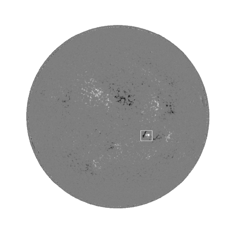
Figure 1: The full Sun observed with SDO/HMI on 2013, June 12th at 23:40UT. The white box marks the active region AR11768, investigated in this paper.

The Sunrise balloon-borne solar observatory (see Barthol et al., 2011; Berkefeld et al., 2011; Gandorfer et al., 2011, for details) carries the vector magnetograph IMaX (Martínez Pillet et al., 2011). Sunrise has flown twice, the first time in 2009 (Solanki et al., 2010, referred to as Sunrise I) when it exclusively observed quiet Sun. These data were inverted by Borrero et al. (2011) using the VFISV code and more recently again, after further refinements, by Kahil et al. (2016) using the SPINOR inversion code (Frutiger et al., 2000). Sunrise flew again in 2013 (referred to as Sunrise II) when it caught an emerging active region. The changes in the instrumentation, the flight, data reduction and inversions are described by Solanki et al. (2016). The atmospheric model for the inversion assumes a hight independent magnetic field vector. In a forthcoming work we plan to use also an MHD-assisted Stokes inversion (leading to a 3D solar atmosphere), as described by Riethmüller et al. (2016).

Figure 1 shows a full disk image of the line-of-sight magnetic field observed with SDO/HMI on 2013, June 12th at 23:40UT and AR11768 is marked with a white box. A part of this AR has been observed with Sunrise II. For the work in this paper we use a data set of 28 IMaX vector magnetograms taken with a cadence of $36.5$s starting on 2013, June 12th at 23:39UT. The data have a pixel size of 40 km and the IMaX-FOV contains $(936\times 936)$ pixel² (about $(37\times 37)$ Mm²). Due to the high spatial resolution of Sunrise/IMaX and a correspondingly small FOV, we embed the data in vector magnetograms observed with SDO/HMI at 23:36UT, 23:48UT and at 00:00UT. The combined data set contains the entire active region, is approximately flux balanced and the total FOV is $(89\times 86)$ Mm². The location of the active region is marked with a white box in Fig. 1.

2.1 Embedding and ambiguity removal

To align the HMI vector maps and IMaX vector magnetogramms we rotate ($\phi\approx-10^{\circ}$) and rescale (by about a factor 9) the HMI-data. The exact values are computed separately for each snapshot by a correlation analysis. From the three HMI vector magnetograms we always choose the one closest in time to the related IMaX snapshot. The horizontal field vectors from HMI are transformed by the rotation to the local coordinates of the IMaX-FOV (see Gary & Hagyard, 1990, for the transformation procedure). We note that this effect is very small for the small rotation angle of $\phi\approx-10^{\circ}$ found here. The correlation between fields with and without taking this effect into account is $98\%$. We remove the $180^{\circ}$ ambiguity in the IMaX data with an acute angle method. See, e.g., Metcalf et al. (2006) for an overview of ambiguity removal methods. The acute angle method minimizes the angle with a reference field, here the corresponding HMI vector magnetograms. The resulting field is shown in Figure 2. On average $13\%\pm 4\%$ of the pixels flip their ambiguity between consecutive snapshots.

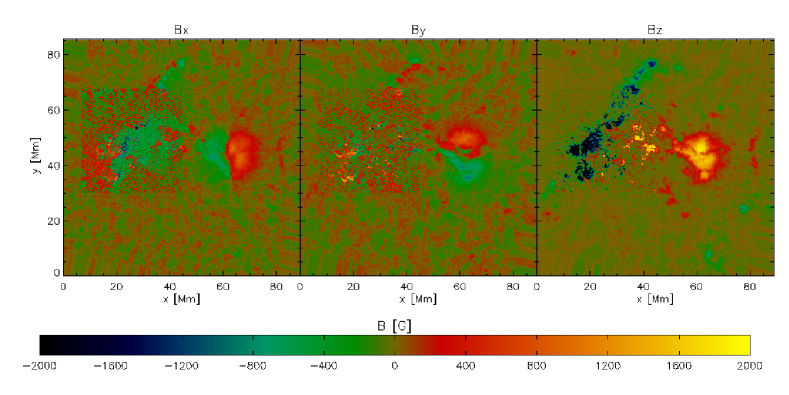
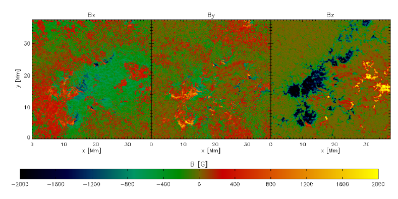
Figure 2: Top: Vector magnetogram of IMaX (first snapshot taken on 2013, June 12th at 23:39UT) embedded in the HMI FOV. The FOV of IMaX is clearly visible due to the better resolved structures. The left and center panels show the horizontal field components $B_{x}$ and $B_{y}$. The right panel corresponds to the vertical field $B_{z}$. Bottom: vector magnetogram for the IMaX FOV. Please note the different x- and y-axes in top and bottom panels.

We note that the chosen HMI magnetograms are almost flux balanced, with an imbalance of $-0.5\%,-1.2\%,-0.5\%$ respectively. The combined data set (IMaX embedded in HMI) shows an imbalance of $-4.2\%\pm-0.5\%$. This is a systematic effect which necessarily appears due to the much higher resolution of IMaX. The net flux is negative, because the FOV of IMaX is located in a mainly negative polarity region. HMI misses a significant amount of small scale magnetic flux, as shown in Fig. 3 (see also the paper by Chitta et al. (2016), who also show that HMI misses a considerable amount of small-scale flux and structure). This difference in the flux measured by the two instruments is a natural result of their different spatial resolutions. The missing small scale flux is due to a cancellation of the Zeeman signals of opposite polarity fields within a resolution element of HMI. The field strength in HMI-magnetograms is lower, because the HMI inversion does not use filling factors.

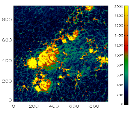
Figure 3: Comparison of the field strength $B$ (only within the FOV of IMaX) for data from HMI (left) and IMaX (right). The x- and y-axes are numbered in pixels. Due to the much higher resolution of IMaX, stronger fields are detected. Naturally this results also in a higher average field strength in the IMaX data: $470G$ than those from HMI: $287G$. Both data-sets have been taken almost at the same time at 23:48UT.

3 Theory

3.1 Magneto-static extrapolation techniques

We use the photospheric vector magnetograms described above as boundary condition for a magneto-static field extrapolation. Therefore we use a special class of separable magneto-static solutions proposed by Low (1991). This model has the advantage of leading to linear equations, which can be solved effectively by a fast Fourier transformation. A corresponding code has been described and applied to a quiet-Sun region observed with Sunrise I in Paper I. Here we only briefly describe the main features of this method and refer to our Paper I for details. The electric current density is described as

$$\nabla\times{\bf B}=\alpha{\bf B}+a\exp(-\kappa z)\nabla B_{z}\times{\bf e_{z}},$$ (1)

where $\alpha$ controls the field aligned currents and $a$ the non-magnetic forces, which compensate the Lorentz-force. Because the solar corona above active regions is almost force-free (see Gary, 2001) the non-magnetic forces have to decrease with height. As in Paper I we choose $\frac{1}{\kappa}=2$ Mm to define the height of the non-force-free domain.

3.2 Using observations to optimize the parameters $\alpha$ and $a$

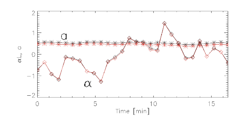
Figure 4: Temporal evolution of $\alpha L$ (diamonds) and $a$ (asterisks) as computed by equations (2) and (5). In black are shown the values computed from the original IMaX vector magnetograms and in red a re-evaluation from the resulting magneto-static equilibria. $t=0$ corresponds to 23:39UT.

In Paper I, $\alpha$ and $a$ were treated as free parameters. For the active region measurements in this paper, we propose to use the horizontal photospheric field vector to constrain $\alpha$ and $a$. This was not possible for the quiet-Sun (QS) region investigated in Paper I, because the poor signal-to-noise-ratio in QS regions does not allow an accurate determination of the horizontal field components. For computing $\alpha$ we follow an approach developed by Hagino & Sakurai (2004) for linear force-free fields:

$$\alpha=\frac{{\sum}{\left(\frac{\partial B_{y}}{\partial x}-\frac{\partial B_{x}}{\partial y}\right){\rm sign}(B_{z})}}{\sum{|B_{z}|}},$$ (2)

where the summation is done over all pixels of the magnetogram. Please note that $\alpha$ has the dimension of an inverse length and the values of $\alpha$ presented in this paper are normalized with $L=37$ Mm, which is the width of the IMaX-FOV. The temporal evolution of $\alpha$ as deduced from Eq. (2) is shown with diamonds in Figure 4. The input (black diamonds) in Fig. 4 and output values (red diamonds) of the global parameter $\alpha$ are almost identical. The small discrepancies that occur are due to numerical errors.

A straightforward way of computing the force parameter $a$ in Eq. (1) is more challenging than computing $\alpha$. While $\alpha$ controls currents which are strictly parallel to the field lines, this is different for the $a$ term. This part controls the horizontal currents and in the generic case these currents are oblique to the magnetic field. This means they have a parallel as well as a perpendicular component. The latter one is responsible for a non-vanishing Lorentz force. We recall (see Molodenskii, 1969; Molodensky, 1974, for details) that the Lorentz force can be written as the volume integral of the divergence of the Maxwell stress tensor $T$:

$$F_{\rm Lorentz}=\int\nabla\cdot T\,dV=\oint T\,ds,$$ (3)

and one gets surface integrals enclosing the volume by applying Gauss’ law. This approach is used frequently in nonlinear force-free computations to check whether a magnetogram is consistent with the force-free criterion. In principle the surface integral has to be taken over the entire surface of the computational volume, but for applications to measurements, one has to restrict it to the bottom, photospheric boundary. We note that neglecting the contribution of lateral boundaries can be more critical for small FOVs like ours than for full ARs surrounded by a weak field skirt. Following a suggestion by Aly (1989), the components of the surface integral (limited to the photosphere) are combined and normalized to define a dimensionless parameter:

$$\epsilon_{{\rm force}}=\frac{\left|{\sum}B_{x}B_{z}\right|+\left|{\sum}B_{y}B_{z}\right|+\left|{\sum}(B_{x}^{2}+B_{y}^{2})-B_{z}^{2}\right|}{{\sum}(B_{x}^{2}+B_{y}^{2}+B_{z}^{2})},$$ (4)

where the summation is done over all pixels of the magnetogram. This parameter is frequently used to check whether a given vector magnetogram is force-free consistent (and can be used as boundary condition for a force-free coronal magnetic field modelling) or if a pre-processing is necessary (see Wiegelmann et al., 2006, 2008, for details). While the pre-processing aims at finding suitable boundary conditions for force-free modelling, the magneto-static approach used here takes the non-magnetic forces into account. While $a$ in Eq. (1) controls the corresponding parts of the current and Eq. (4) is a measure for the non-vanishing Lorentz-force, it is natural to try to relate $a$ and $\epsilon_{{\rm force}}$. Because $a$ is linear in the electric current density, it implicitly also influences the magnetic field, and we cannot assume that the relationship of $a$ and $\epsilon_{{\rm force}}$ is strictly linear. Nevertheless an empirical approach suggests a linear relation to lowest order and one finds that

$$a=2\epsilon_{{\rm force}}$$ (5)

is a reasonable approximation for specifying the free parameter $a$. The black asterisks in Fig. 4 show the temporal evolution of $a$ (or $2\epsilon_{{\rm force}}$) as deduced with Eqs. (4) and (5) from IMaX. We re-evaluate the forces in the photosphere from the resulting magneto-static equilibrium, shown as red asterisks in figure 4. It is found that our special class of linear magneto-static equilibria somewhat underestimates the forces $(15\%\pm 1\%)$ in the lowest photospheric layer. This effect occurs with a low scatter for the entire investigated time series. Possible reasons for this behaviour are the general limitations of applying Eq. (4) to a small FOV, as discussed above. We note that a linear model cannot be assumed to reveal local structures like localized electric currents and horizontal magnetic fields. This is a property which linear magneto-static fields share with linear force-free fields. But the linear magneto-static approach allows considering the non-force-free nature of the lower solar atmosphere as deduced from measurements from equation (4). A linear force-free model would fulfill (2) as well, but $\epsilon_{{\rm force}}$ is zero per definition for force-free models.

4 Results

4.1 3D magnetic field lines

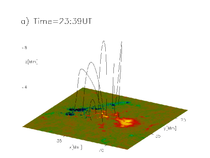
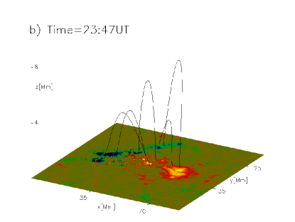
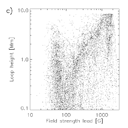
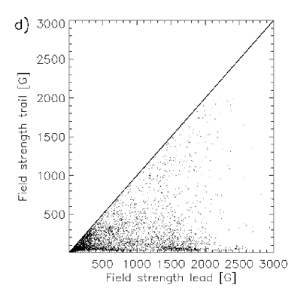
Figure 5: Panels a) and b) show example field lines for the entire (HMI+IMaX) FOV and up to $z=8$ Mm for the first snapshot at 23:39UT and at snapshot 15 at 23:47UT. In panel c) we show for a sample of $10.000$ randomly chosen loops a scatter plot of the strength at the leading foot points and the loop heights at 23:39UT. Panel d) shows a scatter plot of the field strength of the leading (stronger) and trailing (weaker) foot points for loops reaching at least into the chromosphere.

In Fig. 5 we show a few sample field lines at 23:39UT and 23:47UT in panels a) and b), respectively. The field line integration has been started at the same points in negative polarity regions. As one can see some of the larger, coronal loops change their connectivity during this time and connect to different positive polarity regions in both panels. In panel a) the two smallest loops reach into the chromosphere. This is not the case in panel b), where these loops close already at photospheric heights. A detailed analysis of these features is well outside the scope of this paper, however. Further investigations of these low lying structures, also taking Sunrise/SUFI data into account can be found in the paper by Jafarzadeh et al. (2016).

In the following we investigate the relation of the strength of loop foot points and loop heights. Therefor we analyse a sample of 10,000 randomly chosen loops, excluding loops originating in photospheric regions below the the $1\sigma$ noise level of $13$G (the $3\sigma$ noise level is $40G$,see Kaithakkal et al., 2016), those originating in a frame of 150 pixel at the lateral boundaries of the magnetogram, unresolved loops (loop top below $z=100$km) and field lines not closing within the computational domain.

For the snapshots at 23:39 UT (23:47 UT) we found a correlation of the stronger, leading foot point strength and loop height of $51\%(55\%)$ and a correlation of the weaker trailing foot point strength and loop height of $32\%(40\%)$. In Fig. 5c) we show a scatter plot (based on 10,000 loops) of the strength of the leading foot point and height of the loops. In Table 1, deduced from two snapshots at 23:39UT and 23:47UT, we investigate some properties of photospheric, chromospheric and coronal loops. The values hardly change for a larger sample of loops and temporal changes are moderate.

Table 1: The table shows the average field strength at the leading (stronger) and trailing (weaker) foot points for loops reaching into different regions of the solar atmosphere. The first row contains all 10,000 loops, the second row loops closing within photospheric heights (loop top below $z<0.5$Mm), the third row chromospheric loops ($0.5\leq z<2$ Mm) and the fourth row coronal loops ($z\geq 2$Mm). The upper part of the table has been deduced from a snapshot at 23:39UT and the lower part from a snapshot at 23:47UT.

Time	Region	Perc.	lead [G]	trail [G]
23:39UT	all	$100\%$	476	152
23:39UT	photosphere	$39\%$	266	114
23:39UT	chromosphere	$37\%$	395	120
23:39UT	corona	$24\%$	947	263
23:47UT	all	$100\%$	440	147
23:47UT	photosphere	$42\%$	238	107
23:47UT	chromosphere	$39\%$	380	114
23:47UT	corona	$19\%$	995	297

There is a clear tendency that on average both footpoints of coronal loops are stronger than for loops reaching only into the chromosphere or photosphere. While on average the leading footpoint of chromospheric loops is about a factor of $1.5$ stronger than for photospheric loops, one hardly finds a difference for trailing footpoints between photospheric and chromospheric loops.

Fig. 5d) shows a scatter plot of the leading and trailing foot points for loops reaching at least into the chromosphere ($z\geq 500$km). A similar figure was shown in Wiegelmann et al. (2010a), their Fig. 4a, for a quiet Sun region observed during the first flight of Sunrise. For the investigations here, in an active region, we do not find such a strong asymmetry in foot point strength as seen in the quiet Sun. A substantial number of loops are close to the solid line, which corresponds to equal strength of both foot points. For the quiet Sun, symmetric or almost symmetric loops with a leading foot point strength above $800$G have been absent. This is different here and in active regions almost symmetric loops exist even for foot point strengths of $2000$G and above. As the scatter plot Fig. 5d) and Table 1 show, the majority of the active region loops has foot points with different strength, but this effect is much less pronounced compared with quiet Sun loops shown in Wiegelmann et al. (2010a) Fig. 4a).

4.2 Plasma

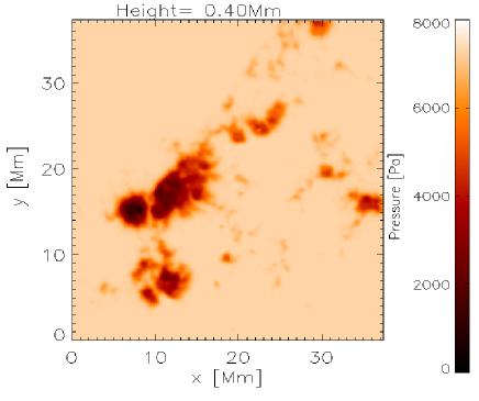
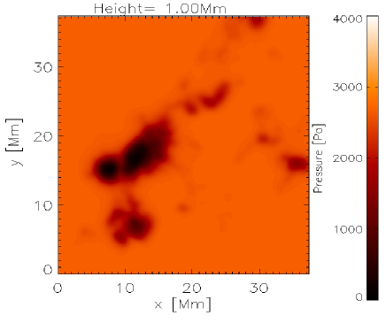
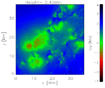
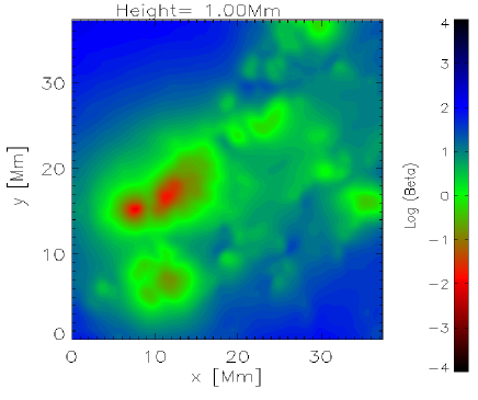
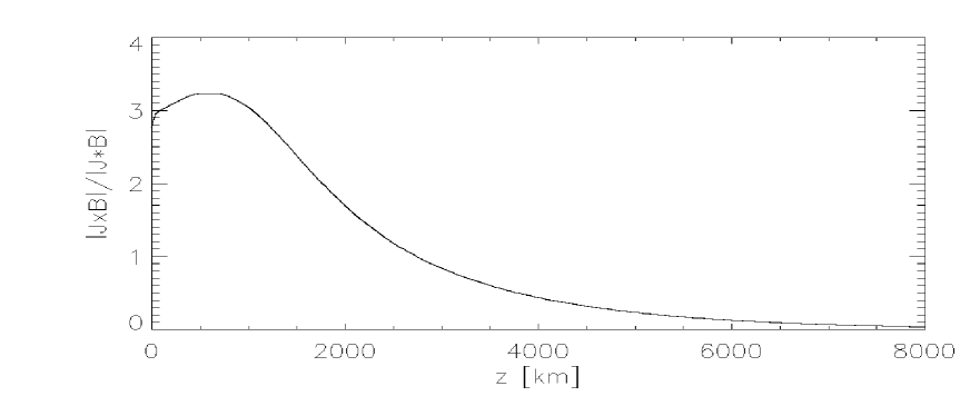
Figure 6: Plasma pressure (top panels) and plasma $\beta$ (center panels) at height $400$ km and $1$ Mm for the first snapshot at 23:39UT. The bottom panels shows the averaged Lorentz force $\frac{|{\bf J}\times{\bf B}|}{|{\bf J}\cdot{\bf B}|}$ as a function of hight.

Following Paper I the plasma pressure $p$ and density $\rho$ are divided into two parts, which are computed separately and then added together. The non-vanishing Lorentz force is compensated by the gradient of the plasma pressure and in the vertical direction also partly by the gravity force. We compute the corresponding part of the plasma pressure $p$ and density $\rho$ following the explanations given in Paper I. Superimposed on this component a background plasma (obeying a 1D-equilibrium of pressure gradient and gravity in the vertical direction) is added to ensure a total positive density and pressure. The top panels in Fig. 6 show the plasma pressure in the upper photosphere (height $z=400$ km) and mid chromosphere ($z=1$ Mm) for one snapshot from the beginning of the time series. The center panels in Fig. 6 show the plasma $\beta$ for the same heights. The overall structure of these quantities, here shown for only one snapshot, vary only very moderately in time. A low plasma $\beta$ is a sufficient, but not necessary condition for a magnetic field to be force-free. To test whether our fields really are non-force-free, we show the horizontal averaged Lorentz force as a function of height in the bottom panel of Fig. 6. Shown is the dimensionless quantity $\frac{|{\bf J}\times{\bf B}|}{|{\bf J}\cdot{\bf B}|}$, which compares the importance of perpendicular and field aligned electric currents. The quantity becomes zero for a vanishing Lorentz force. In the lower atmosphere the perpendicular currents dominate (i.e., $|{\bf J}\times{\bf B}|>|{\bf J}\cdot{\bf B}|$) and there relative influence is maximum at $z=600$km. Towards coronal heights, field aligned currents dominate (i.e., $|{\bf J}\times{\bf B}|\ll|{\bf J}\cdot{\bf B}|$).

For the quiet-Sun region in Paper I it was found that the used special class of magneto-static equilibria are not flexible enough to model the full FOV with a unique set of parameters $\alpha$ and $a$. The reason was that strongly localized magnetic elements in an otherwise weak-field quiet-Sun area were incompatible with the intrinsic linearity of the underlying equations. Similar limitations do not occur, however, for the active region investigated in this paper. The magnetic field of the large scale pore (shown in dark blue in figure 2) can be modelled significantly better with the linear approach than the localized magnetic elements in Paper I. Furthermore, as explained in section 3.2, $\alpha$ and $a$ can be deduced from measurements, which was not possible in the quiet Sun.

4.3 Comparison with potential and force-free model

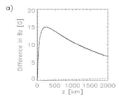
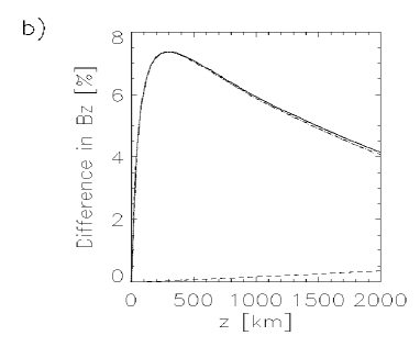
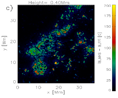
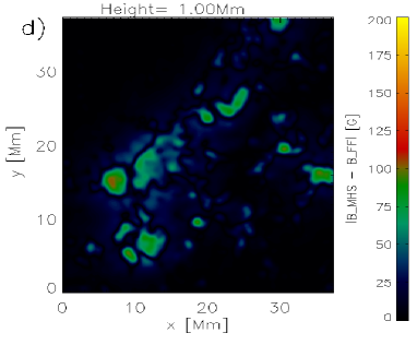
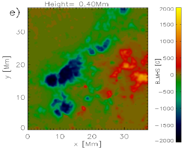
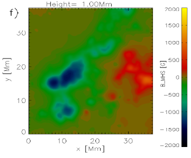
Figure 7: a) Comparison of the vertical magnetic flux $z\rightarrow B_{z}(z)$ computed with different models. Average difference in G of magneto-static (with $a=0.55$ and $\alpha L=-0.7$) and linear-force-free (with $\alpha L=-0.7$ model (solid line), magneto-static and potential field model (dash-dotted line) and linear force-free and potential field model (dashed line). b) Same as panel a), but the differences have been normalized with the averaged absolute magnetic flux at every height $z$. Panels c) and d) show the absolute differences of the vertical magnetic field between a magneto-static and linear-force-free model in the height $400$ km and $1$ Mm, respectively. Panels e) and f) show $B_{z}$ of the MHS-model at the same heights. All panels correspond to the first snapshot from IMaX at 23:39UT.

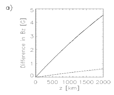
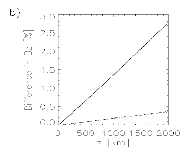
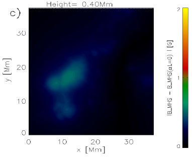
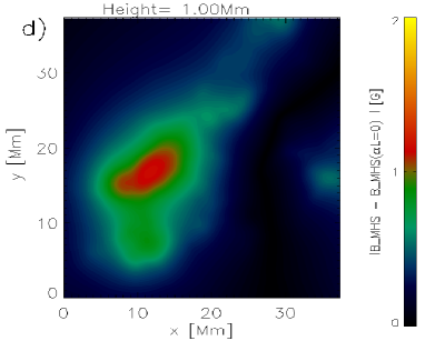
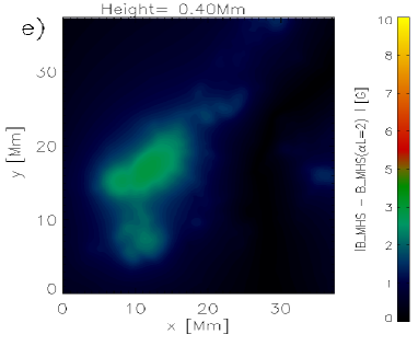
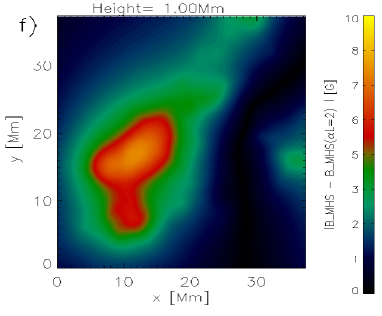
Figure 8: a) Comparison of the vertical magnetic flux $z\rightarrow B_{z}(z)$ computed with magneto-static models with different values of $\alpha$. We show the average difference in G of the original magneto-static model $\alpha L=-0.7$ and a MHS-model with $\alpha L=0.0$ (dashed line) and $\alpha L=2.0$ (solid line). b) Same as panel a), but the differences have been normalized with the averaged absolute magnetic flux at every height $z$. Panels c) and d) show the absolute differences of the vertical magnetic field between the MHS-models with $\alpha L=-0.7$ and $\alpha L=0.0$ at the height $400$ km and $1$ Mm, respectively. Panels e) and f) show a comparison of MHS-models with $\alpha L=-0.7$ and $\alpha L=2.0$. Please note the different colour scales.

Simpler than magneto-static extrapolations are potential and linear force-free models. Here we would like to point out some differences. In Fig. 7 panel a) we show the average difference in vertical field strength $B_{z}$ as a function of the height $z$ in the solar atmosphere. The dashed line compares the result of a potential and linear force-free model. As one can see the differences are very small and increase linearly with height. This property was already found for the quiet Sun in Wiegelmann et al. (2010a). The solid and dash-dotted lines compare the magneto-static model with linear-force-free and potential fields, respectively. Both lines almost coincide at low heights and differ only slightly higher. We find that the magneto-static model deviates strongest from the other models at a height $z=240$ km. In panel b) the differences in $B_{z}$ have been normalized with the (decreasing) average magnetic flux at every height. The curves show, however, the same trend as for the absolute values, just the largest difference is slightly shifted to $z=280$ km. While this horizontal averaged differences are with a maximum of about $15$ G and $7\%$ relatively small, the local deviation is significant, see Fig. 7 panels c) and d), which show the difference of magneto-static and force-free field at a height of $z=400$ km and $z=1$ Mm, respectively. It is not accidental that the differences in the vertical flux between the magneto-static and the force-free model depict a somewhat similar structure as the plasma pressure $p$ and the plasma $\beta$ shown in Fig. 6, because horizontal structures in the plasma are the result of compensating a non-vanishing Lorentz-force. The reason is that for strictly force-free configurations the Lorentz force vanishes and consequently the pressure gradient force has to be compensated by the gravity force alone. Because the gravity force is only vertical in $z$, the pressure cannot vary in the horizontal direction for force-free configurations. Horizontal variations of the pressure, as shown in the top panels of Fig. 6 occur in MHS-solutions, because the pressure gradient force has to compensate the Lorentz force. Consequently structures in the plasma occur in regions where force-free and magneto-static models differ most. In panels e) and f) of Fig. 7 we show for comparison the distribution of $B_{z}$ at the same heights. As one can see, the maximum differences in $B_{z}$ are well below the maximum values of the vertical field (by about a factor of ten). The largest differences are in regions where $B_{z}$ is strong and consequently the plasma pressure and plasma $\beta$ are low.

4.4 Influence of the linear force-free parameter $\alpha$ on MHS equilibria.

As one can see in Fig. 4, $\alpha L$ seems to vary significantly in time and obtains values in the range $\pm 2$. Here we would like to investigate to which extend modifying the parameter $\alpha L$ affects the solution. To do so, we compare (only for the first snapshot) our original linear magneto-static solution with the deduced parameters $a=0.55$ and $\alpha L=-0.7$ with configurations, where $\alpha L$ has been modified to $\alpha L=0.0$ and $\alpha L=+2.0$, respectively.

In Fig. 8a) we show the average difference in vertical field strength $B_{z}$ as a function of the height $z$ in the solar atmosphere. Panel b) shows relative values normalized with averaged absolute magnetic flux at every height $z$. The solid (dotted) lines compare the original MHS-equilibria with the $\alpha L=+2.0$ ($\alpha L=0.0$) ones, respectively. Naturally a larger discrepancy of $\alpha$ results in larger difference of the resulting fields. The influence is, however, much smaller than the comparison of MHS-equilibria and potential and linear force-free fields shown in Fig. 7. A major difference is, however, that the discrepancy of MHS-solutions with different values of $\alpha$ increase with height. Such a property is well known already from the comparison of potential and linear force-free fields in Wiegelmann et al. (2010a). In the top panels of Fig. 8(a and b) we overplot again the difference of a linear force-free field with $\alpha L=-0.7$ and a potential field with $\alpha L=0.0$ with dotted lines. (This quantity was shown already in Fig. 7 with a different axis scale). The dotted and dashed line almost coincide (about $5\%$ difference) and we can conclude that modifying $\alpha$ in MHS-equilibria has a a similar effect as in linear force-free configurations. Fig. 8 panels c-f show the differences of the MHS-solutions in the height $400$km and $1$Mm, respectively. These images should be compared with the corresponding panels in Fig. 7, but please note the very different colour scales (by a factor of 100 between panels c,d in Figs. 7 and 8 and by a factor of 20 between panels c,d in Figs. 7 and panel e,f in Fig. 8). For low-lying structures the influence of changing $\alpha$ is therefor very small. Far more important for the structure in photospheric and chromospheric heights is the force parameter $a$.

5 Discussion and outlook

Within this work we applied a special class of magneto-static equilibria to model the solar atmosphere above an active region. As boundary condition we used measurements of the photospheric magnetic field vector obtained by Sunrise/IMaX, which have been embedded into SDO/HMI active-region magnetograms. The used approach models the 3D magnetic field in the solar atmosphere self-consistently with the plasma pressure and density.

Pressure gradient and gravity forces are important only in a relatively thin (about 2 Mm) layer containing the photosphere and chromosphere. Thanks to the high spatial resolution of IMaX, we were able to resolve this non-force-free layer with $50$ grid points. In Paper I we discussed the limitations of applying our model to the quiet Sun, where strong localized flux elements make a linear approach less favourable. While, in principle, nonlinear models are generically more flexible, we found the active region investigated here to be far more suitable for a linear model than the quiet Sun. In particular, the entire domain could be modelled without running into problems with negative densities and pressures that plagued the application to the quiet Sun. We derived free model parameters from IMaX and a unique set of these parameters was used in the entire modelling domain. The parameter $\alpha$ controls field aligned currents and the parameter $a$ horizontal currents. While the currents controlled by $a$ are strictly horizontal, they have a field line parallel part and a part perpendicular to the field. The latter one is responsible for the finite Lorentz-force and deviation from force-freeness.

Nevertheless, a linear magneto-static model can only be a lowest order approximation. Shortcomings of any linear approach is that the generic non-linear nature of most physical systems is not taken into account. For equilibria in the solar atmosphere this means that strong current concentrations and derived quantities like the spatial distribution of $\alpha(x,y)$ are not modelled adequately. The situation is somewhat similar to the history of force-free coronal models, where linear force-free active region models have been routinely used (see,e.g. Seehafer, 1978; Gary, 1989; Demoulin & Priest, 1992; Demoulin et al., 1992; Wiegelmann & Neukirch, 2002; Marsch et al., 2004; Tu et al., 2005) before nonlinear force-free models entered the scene. Nonlinear magneto-static extrapolation codes have been developed and tested with synthetic data in Wiegelmann & Neukirch (2006); Wiegelmann et al. (2007); Gilchrist et al. (2016). While, in principle, it is straight forward to apply these models to data from Sunrise/IMaX, the implementation details are still challenging, just as this was the case about a decade ago for nonlinear force-free models. A number of problems still need to be solved before nonlinear magneto-static equilibria can be reliably calculated and such models can be routinely applied to solar data. Two issues remain open and are to be dealt with for applying nonlinear magneto-static models to data: i) the noise in photospheric magnetograms, and ii) the problem that the plasma $\beta$ varies over orders of magnitude within the computational volume, which slows down the convergence rate of such codes (see Wiegelmann & Neukirch, 2006, for details). That magneto-static codes are slower than corresponding force-free approaches has been reported also recently in Gilchrist et al. (2016) for a Grad-Rubin like method.

Linear magneto-static equilibria, as computed in this work, can serve as initial conditions for nonlinear computations. Last but not least, one should understand the transition from magneto-static to force-free models above the mid chromosphere. While, in principle, the magneto-static approach includes the force-free one automatically for $\beta\rightarrow 0$, the computational overhead of computing magneto-static equilibria in low $\beta$ regions is severe. In low $\beta$ regions, force-free codes can be applied because the back-reaction of the plasma onto the magnetic field is small and the numerical convergence is faster.

In this paper we applied a linear magneto-static model to compute the magnetic field in the solar atmosphere above an active region. We modelled the mixed $\beta$ layer of photosphere and chromosphere, which required high resolution photospheric field measurements as boundary condition. This work is the second part of applying a linear magneto-static model to high resolution photospheric measurements. In Paper I the model was applied to the quiet Sun. The quiet Sun is composed of small, concentrated (strong) magnetic elements and large inter-net-work regions with weak magnetic field in the photosphere. This property is a challenge to the linear magneto-static model, because the plasma pressure disturbances caused by strong and strongly localized magnetic elements, require a background pressure, which results in an unrealistic high average plasma $\beta$. As pointed out in Paper I the model can be applied locally around magnetic elements, but does not permit a meaningful modelling of large quiet-Sun areas containing magnetic elements of very different strengthes. Strong localization of magnetic elements and the linearity of the model are a contradiction. In active regions, large magnetic pores and sunspots dominate the magnetic configuration. The wider coverage by strong fields in active regions is more consistent with the limitations of a linear model. Furthermore the free model parameters $\alpha$ and $a$ can be deduced from horizontal magnetic field measurements in active regions, which was not possible in the quiet Sun, due to the poor signal-to-noise ratio.

References

- Aly (1989) Aly, J. J. 1989, Sol. Phys., 120, 19
- Amari & Aly (2010) Amari, T. & Aly, J.-J. 2010, A&A, 522, A52
- Amari et al. (1997) Amari, T., Aly, J. J., Luciani, J. F., Boulmezaoud, T. Z., & Mikic, Z. 1997, Sol. Phys., 174, 129
- Aulanier et al. (1999) Aulanier, G., Démoulin, P., Mein, N., et al. 1999, A&A, 342, 867
- Aulanier et al. (1998) Aulanier, G., Demoulin, P., van Driel-Gesztelyi, L., Mein, P., & Deforest, C. 1998, A&A, 335, 309
- Barthol et al. (2011) Barthol, P., Gandorfer, A., Solanki, S. K., et al. 2011, Sol. Phys., 268, 1
- Berkefeld et al. (2011) Berkefeld, T., Schmidt, W., Soltau, D., et al. 2011, Sol. Phys., 268, 103
- Borrero & Kobel (2011) Borrero, J. M. & Kobel, P. 2011, A&A, 527, A29
- Borrero & Kobel (2012) Borrero, J. M. & Kobel, P. 2012, A&A, 547, A89
- Borrero et al. (2011) Borrero, J. M., Tomczyk, S., Kubo, M., et al. 2011, Sol. Phys., 273, 267
- Chitta et al. (2016) Chitta, L. P., Peter, H., Solanki, S. K., et al. 2016, ApJS in press
- Demoulin & Priest (1992) Demoulin, P. & Priest, E. R. 1992, A&A, 258, 535
- Demoulin et al. (1992) Demoulin, P., Raadu, M. A., & Malherbe, J. M. 1992, A&A, 257, 278
- DeRosa et al. (2009) DeRosa, M. L., Schrijver, C. J., Barnes, G., et al. 2009, ApJ, 696, 1780
- DeRosa et al. (2015) DeRosa, M. L., Wheatland, M. S., Leka, K. D., et al. 2015, ApJ, 811, 107
- Frutiger et al. (2000) Frutiger, C., Solanki, S. K., Fligge, M., & Bruls, J. H. M. J. 2000, A&A, 358, 1109
- Gandorfer et al. (2011) Gandorfer, A., Grauf, B., Barthol, P., et al. 2011, Sol. Phys., 268, 35
- Gary (1989) Gary, G. A. 1989, ApJS, 69, 323
- Gary (2001) Gary, G. A. 2001, Sol. Phys., 203, 71
- Gary & Hagyard (1990) Gary, G. A. & Hagyard, M. J. 1990, Sol. Phys., 126, 21
- Gilchrist et al. (2016) Gilchrist, S. A., Braun, D. C., & Barnes, G. 2016, Sol. Phys., tmp..182G
- Hagino & Sakurai (2004) Hagino, M. & Sakurai, T. 2004, PASJ, 56, 831
- Jafarzadeh et al. (2016) Jafarzadeh, S., Rutten, R. J., Solanki, S. K., et al. 2016, ApJS in press
- Kahil et al. (2016) Kahil, F., Riethmüller, T. L., & Solanki, S. K. 2016, ApJS in press
- Kaithakkal et al. (2016) Kaithakkal, A. J., Riethmüller, T. L., Solanki, S. K., et al. 2016, ApJS in press
- Khomenko & Collados (2008) Khomenko, E. & Collados, M. 2008, ApJ, 689, 1379
- Low (1991) Low, B. C. 1991, ApJ, 370, 427
- Marsch et al. (2004) Marsch, E., Wiegelmann, T., & Xia, L. D. 2004, A&A, 428, 629
- Martínez Pillet et al. (2011) Martínez Pillet, V., Del Toro Iniesta, J. C., Álvarez-Herrero, A., et al. 2011, Sol. Phys., 268, 57
- Metcalf et al. (1995) Metcalf, T. R., Jiao, L., McClymont, A. N., Canfield, R. C., & Uitenbroek, H. 1995, ApJ, 439, 474
- Metcalf et al. (2006) Metcalf, T. R., Leka, K. D., Barnes, G., et al. 2006, Sol. Phys., 237, 267
- Molodenskii (1969) Molodenskii, M. M. 1969, Soviet Ast., 12, 585
- Molodensky (1974) Molodensky, M. M. 1974, Sol. Phys., 39, 393
- Pesnell et al. (2012) Pesnell, W. D., Thompson, B. J., & Chamberlin, P. C. 2012, Sol. Phys., 275, 3
- Petrie (2000) Petrie, G. J. D. 2000, PhD thesis, Department of Mathematics and Statistics, University of St. Andrews, Scotland
- Petrie & Neukirch (2000) Petrie, G. J. D. & Neukirch, T. 2000, A&A, 356, 735
- Riethmüller et al. (2016) Riethmüller, T. L., Solanki, S. K., Barthol, P., et al. 2016, ApJS in press
- Scherrer et al. (2012) Scherrer, P. H., Schou, J., Bush, R. I., et al. 2012, Sol. Phys., 275, 207
- Schrijver et al. (2008) Schrijver, C. J., DeRosa, M. L., Metcalf, T., et al. 2008, ApJ, 675, 1637
- Seehafer (1978) Seehafer, N. 1978, Sol. Phys., 58, 215
- Solanki et al. (2010) Solanki, S. K., Barthol, P., Danilovic, S., et al. 2010, ApJ, 723, L127
- Solanki et al. (2016) Solanki, S. K., Riethmüller, T. L., Barthol, P., et al. 2016, ApJS in press
- Tu et al. (2005) Tu, C.-Y., Zhou, C., Marsch, E., et al. 2005, Science, 308, 519
- Wheatland & Régnier (2009) Wheatland, M. S. & Régnier, S. 2009, ApJ, 700, L88
- Wiegelmann et al. (2006) Wiegelmann, T., Inhester, B., & Sakurai, T. 2006, Sol. Phys., 233, 215
- Wiegelmann & Neukirch (2002) Wiegelmann, T. & Neukirch, T. 2002, Sol. Phys., 208, 233
- Wiegelmann & Neukirch (2006) Wiegelmann, T. & Neukirch, T. 2006, A&A, 457, 1053
- Wiegelmann et al. (2015) Wiegelmann, T., Neukirch, T., Nickeler, D. H., et al. 2015, ApJ, 815, 10
- Wiegelmann et al. (2007) Wiegelmann, T., Neukirch, T., Ruan, P., & Inhester, B. 2007, A&A, 475, 701
- Wiegelmann & Sakurai (2012) Wiegelmann, T. & Sakurai, T. 2012, Living Reviews in Solar Physics, 9, 5
- Wiegelmann et al. (2010a) Wiegelmann, T., Solanki, S. K., Borrero, J. M., et al. 2010a, ApJ, 723, L185
- Wiegelmann et al. (2008) Wiegelmann, T., Thalmann, J. K., Schrijver, C. J., De Rosa, M. L., & Metcalf, T. R. 2008, Sol. Phys., 247, 249
- Wiegelmann et al. (2014) Wiegelmann, T., Thalmann, J. K., & Solanki, S. K. 2014, A&A Rev., 22, 78
- Wiegelmann et al. (2010b) Wiegelmann, T., Yelles Chaouche, L., Solanki, S. K., & Lagg, A. 2010b, A&A, 511, A4