Toward an Effective Field Theory Approach to Reheating

Abstract

We investigate whether Effective Field Theory (EFT) approaches, which have been useful in examining inflation and dark energy, can also be used to establish a systematic approach to inflationary reheating. We consider two methods. First, we extend Weinberg’s background EFT to the end of inflation and reheating. We establish when parametric resonance and decay of the inflaton occurs, but also find intrinsic theoretical limitations, which make it difficult to capture some reheating models. This motivates us to next consider Cheung, et. al.’s EFT approach, which instead focuses on perturbations and the symmetry breaking induced by the cosmological background. Adapting the latter approach to reheating implies some new and important differences compared to the EFT of Inflation. In particular, there are new hierarchical scales, and we must account for inflaton oscillations during reheating, which lead to discrete symmetry breaking. Guided by the fundamental symmetries, we construct the EFT of reheating, and as an example of its usefulness we establish a new class of reheating models and the corresponding predictions for gravity wave observations. In this paper we primarily focus on the first stages of preheating. We conclude by discussing challenges for the approach and future directions. This paper builds on ideas first proposed in the note Ozsoy:2015rna .

I Introduction

If inflation occurred in the early universe it must have eventually ended resulting in a hot, thermal universe by the time of Big Bang Nucleosynthesis (BBN). The process by which the inflaton’s energy is transferred into other particles – which hopefully, eventually, gave rise to Standard Model particles – is known as inflationary reheating. Reheating can occur perturbatively Abbott:1982hn ; Albrecht:1982mp ; Dolgov:1982th , or non-perturbatively in a process known as preheating Dolgov:1989us ; Traschen:1990sw ; Kofman:1997yn (see Amin:2014eta ; Allahverdi:2010xz for recent reviews).

Existing investigations into reheating have been rather model dependent, often focusing on constraining the precise regions of the parameter space that lead to successful reheating. Analytic methods for exploring the dynamics still rely on the earliest works mentioned above, and the non-linearities and complexity of the reheating process still require invoking numeric/lattice methods Khlebnikov:1996mc ; Easther:2006gt ; GarciaBellido:1997wm ; Felder:2000hj ; Easther:2006vd ; Price:2008hq ; Easther:2010qz ; Amin:2014eta ; Allahverdi:2010xz . Moreover, the wealth of cosmological observations from the Cosmic Microwave Background (CMB) and Large Scale Structure (LSS) relate to the physics of inflation far before reheating, and so the lack of observational windows on (p)reheating has also made its study far less compelling than inflation – with the prediction of gravitational waves providing a possible exception.

In this paper, we take steps to address the model dependence of (p)reheating building on motivation from recent works Hertzberg:2014iza ; Amin:2015ftc ; Ozsoy:2015rna . Our approach is to use the Effective Field Theory (EFT) approach to cosmology, which at this point has been applied to all cosmic epochs except for (p)reheating. We will first consider the EFT of the background as developed by Weinberg for inflation in Weinberg:2008hq and later adapted to studies of dark energy in Park:2010cw . Ultimately, we will find that this approach is not completely satisfactory in generalizing studies of reheating. Instead we find that the different approach of the EFT of cosmological perturbations is more promising.

The EFT of Inflation Creminelli:2006xe ; Cheung:2007st ; Senatore:2010wk and generalizations to dark energy Creminelli:2008wc ; Bloomfield:2012ff ; Gubitosi:2012hu ; Fasiello:2016qpn ; Fasiello:2016yvr ; Lewandowski:2016yce and structure formation Baumann:2010tm are based on the idea that there is a physical clock corresponding to the Goldstone boson that non-linearly realizes the spontaneously broken time diffeomorphism invariance of the background. In unitary gauge – where the clock is homogeneous – the matter perturbations are encoded within the metric, i.e. the would-be Goldstone boson is ‘eaten’ by the metric, since gravity is a gauge theory. After we establish the limitations of the EFT background approach, we then present an EFT of reheating using this EFT of perturbations to develop a more robust approach to studying the end of inflation and reheating.

The rest of the paper is as follows. In Section II, we review some of the important issues and constraints surrounding particular examples of (p)reheating models. In Section III, we consider Weinberg’s approach to the EFT of Inflation, and consider how inflation might end and (p)reheating would proceed. We find that the perturbative approach to the background presents a substantial challenge to this approach, along with the usual problem of knowing the complete inflationary potential. This motivates us to construct an EFT of reheating in Section IV – focusing on the EFT of the perturbations. We analyze the process of particle production, demonstrate how our approach connects to existing preheating models, and discuss ways in which our EFT can be used to connect to both inflation (and its end) and observations. In Section V, we conclude and discuss the challenges facing our approach and future directions.

II Challenges for Inflationary Reheating

Model dependent studies of (p)reheating have raised a number of important questions and issues. From the perspective of inflationary model building within string theory, the requirement to isolate the inflationary sector to achieve an adequate duration of inflation can result in challenges in transferring the energy density to other fields, and eventually the Standard model sector following inflation Kofman:2005yz . The complexity of the string landscape and the large number of moduli fields can exacerbate this problem Green:2007gs . In bottom-up approaches, toy models often demonstrate a conflict between the need for the inflaton to have feeble interactions during inflation (so as to be consistent with both successful inflation and constraints on non-Gaussianity), and later having strong enough couplings for the complete decay of the inflaton and the (eventual) successful reheating of the Standard Model. Perturbative decay can also present a challenge depending on the effective mass of the decay channels and the time dependence of the inflaton decay rate Felder:1998vq .

As an example, consider Chaotic inflation with $V\sim m^{2}_{\phi}\phi^{2}$ and reheating with a renormalizable coupling to a reheat field, $\chi$. We note that this model is in tension with existing CMB constraints, but it presents a simple example of the more general problems one might anticipate with (p)reheating. The Lagrangian we consider is

$${\cal L}=-\frac{1}{2}\left(\partial\phi\right)^{2}-\frac{1}{2}m_{\phi}^{2}\phi^{2}-\frac{1}{2}\left(\partial\chi\right)^{2}-U(\chi)-\frac{g^{2}}{2}\phi^{2}\chi^{2},$$ (1)

where we assume that initially the reheat field is fixed by its $U(\chi)$ and remains in its vacuum during inflation. The mass of the inflaton is fixed by the power spectrum Ade:2015lrj ,

$$\Delta_{\mathcal{R}}^{2}=\frac{1}{96\pi^{2}}\left(\frac{m_{\phi}}{m_{\rm pl}}\right)^{2}\left(4N_{*}\right)^{2}\equiv 2.2\times 10^{-9}$$ (2)

where $N_{*}$ is the number of e-folds before the end of inflation and with $N_{*}=60$ we have $m_{\phi}\simeq 6.4\times 10^{-6}\,m_{\rm pl}$. The inflaton will begin to oscillate around the minimum of its potential when its mass becomes comparable to the Hubble scale, $m_{\phi}\approx H(t_{\rm{\mbox{\tiny osc}}})$, with a profile given by the expression $\phi_{0}(t)=\Phi(t)\sin(m_{\phi}t)$ Kofman:1997yn . The amplitude of the oscillations, $\Phi(t)$, is a monotonic function of cosmic time given by $\Phi=\sqrt{8/3}~{}(m_{\rm pl}/2\pi N_{\rm{\mbox{\tiny osc}}})$, where $N_{\rm{\mbox{\tiny osc}}}$ is the number of oscillations after the end of inflation. Setting $N_{\rm{\mbox{\tiny osc}}}=1$ gives $\Phi\approx 0.3\,m_{\rm pl}$, which we take as the initial amplitude of the inflaton oscillations.

If the direct coupling in (1) presents the only decay channel for the inflaton the expansion of the universe will prevent the complete perturbative decay of the inflaton Kofman:1997yn . This is because the decay rate, $\Gamma$, scales as $\Gamma\propto\Phi^{2}\sim 1/t^{2}$ whereas the expansion rate during reheating scales as $H\sim 1/t$. Instead, in this case decay must proceed non-perturbatively through preheating Dolgov:1989us ; Traschen:1990sw ; Kofman:1997yn , where parametric resonance can lead to enhanced decay of the inflaton condensate. The mode equation for $\chi$ fluctuations resulting from (1) in the presence of the oscillating condensate $\phi_{{}_{0}}(t)$ is

$$\ddot{\chi}_{k}+\left[k^{2}+m_{\chi}^{2}+g^{2}\phi_{{}_{0}}^{2}\right]\chi_{k}=0,$$ (3)

where we have neglected the expansion of the universe ($a=1$) and note that including gravitational effects would act to strengthen the main conclusion below. If the field begins in its Bunch-Davies vacuum the corresponding WKB solution is $\chi_{k}\sim\exp(-i\int\omega_{k}(t^{\prime})dt^{\prime})$, where $\omega_{k}$ is time-dependent frequency corresponding to the terms inside the brackets in (3). Particle production occurs if the adiabatic conditions fail corresponding to $\dot{\omega}_{k}\gg\omega_{k}^{2}$ or $\ddot{\omega}_{k}\gg\omega_{k}^{3}$, etc… Thus, a necessary condition for preheating is

$$\frac{\dot{\omega}_{k}}{\omega_{k}^{2}}\simeq\frac{g^{2}\phi\dot{\phi}}{\left(k^{2}+m_{\chi}^{2}+g^{2}\phi^{2}\right)^{3/2}}>1,$$ (4)

corresponding to the production of modes with their momenta satisfying

$$k^{2}\lesssim\left(g^{2}\phi\dot{\phi}\right)^{2/3}-g^{2}\phi^{2}-m_{\chi}^{2}.$$ (5)

The ratio in (4) is maximal when the inflaton is near the bottom of the potential, where we can approximate $\dot{\phi}_{0}\simeq m_{\phi}\Phi$. Broad resonance Kofman:1997yn will assure us that preheating is successful. This corresponds to a restriction on the range of wave numbers in the resonance band $\Delta k\gg m_{\phi}$ Maximizing the right side of (5) with respect to $\phi$, we find the maximum value of $\phi_{*}^{2}\simeq 0.2\,\dot{\phi}/g$ corresponding to a maximum value of resonant momentum $k^{2}_{\ast}=0.4\,g\dot{\phi}-m_{\chi}^{2}$. Therefore the condition for broad resonance $\Delta k\simeq k_{\ast}\gg m_{\phi}$ can be written as a condition on the coupling constant $g$,

$$g\gg\frac{m_{\phi}^{2}+m_{\chi}^{2}}{\dot{\phi}}\simeq\frac{m_{\phi}^{2}+m_{\chi}^{2}}{m_{\phi}\Phi}.$$ (6)

Taking $\Phi\simeq 0.3\,m_{\rm pl}$ and assuming $m_{\chi}\ll m_{\phi}$ we find $g\gg 3.8\times 10^{-5}$ for efficient preheating in the broad resonance regime.

On the other hand, we can obtain a lower bound on the strength of the coupling by requiring the one-loop correction induced by the $g^{2}\phi^{2}\chi^{2}$ interaction to not to spoil the flatness of the potential during inflation. That is, we require $\delta m_{\phi}\lesssim m_{\phi}\simeq 6.4\times 10^{-6}\,m_{\rm pl}$, whereas the loop correction is $\delta m^{2}_{\phi}=(g^{2}\Lambda_{\rm uv}^{2})/(16\pi^{2})$. The cut-off is expected to be Planckian $\Lambda_{\rm uv}\approx m_{\rm pl}$, implying $g<10^{-5}$. Clearly, this result implies that the required value of the coupling, $g$, to obtain efficient preheating is inconsistent with having a naturally light inflaton during inflation. In other words, in general it is expected that heavy $\chi$ fields running in the loops induced by the direct coupling $g^{2}\phi^{2}\chi^{2}$ tends to de-stabilize parameters of the inflationary sector if we insist on the effective particle production at the end of inflation.

We have a good understanding of the limitations to the approximations we have used above to constrain preheating in chaotic inflation models, especially since these toy models have been well-studied over the years to establish when they lead to successful reheating. At the same time, it is clear that we are seeing tension in analytic expectations for finding reliable preheating models. It is also clear that doing a full non-linear analyses for all parameters in all models of preheating is not an efficient way to do model analysis. Can one always establish a connection between the parameters during inflation and those same parameters during reheating? What is the expected mass of the reheat fields during inflation? Can’t the inflaton just decay through higher dimensional operators present at the time of reheating? These are some of the questions we hope to address by developing a more systematic approach to reheating below.

III Reheating in Weinberg’s Covariant formulation of the EFT of Inflation

In this section, we extend Weinberg’s EFT approach to inflation Weinberg:2008hq to include the end of inflation and the beginning of (p)reheating. Focusing on a two-field scalar field model for simplicity, we present both analytic and numeric results from our investigation into the background evolution and the resulting particle production. We find that consistency of the background EFT within this approach limits its applicability and how well it can be used to successfully describe (p)reheating. This will motivate us to consider a different approach in Section IV.

III.1 Construction of the EFT

Following Weinberg:2008hq we consider the most general EFT of a scalar field in General Relativity which can be written as

$${\cal L}_{\rm inf}=-\frac{1}{2}m_{\rm pl}^{2}R-\frac{1}{2}\left(\partial\phi\right)^{2}-V(\phi)+\frac{c_{1}}{\Lambda^{4}}\left(\partial\phi\right)^{4},$$ (7)

where $\Lambda$ is the UV cutoff of the theory, in general $c_{1}=c_{1}(\phi)$ is an arbitrary function of the scalar, and we have neglected terms involving the Weyl tensor which are suppressed relative to the leading correction Weinberg:2008hq . Assuming that the equations of motion admit inflationary solutions it was shown in Weinberg:2008hq that this is also the most general EFT for the inflationary background (to be contrasted to the EFT for the perturbations which we will discuss in Section IV).

CMB observations imply that the power spectrum of scalar fluctuations is nearly scale-invariant, which can be realized through an approximate shift symmetry for the inflaton. This allows us to approximate $c_{1}(\phi)$ as nearly constant during inflation (its time evolution is slow-roll suppressed). When the EFT expansion is applicable, i.e. $\Lambda>\dot{\phi}^{1/2}$, self-interactions of the inflaton are small and non-Gaussianity is negligible Maldacena:2002vr .

We now introduce an additional scalar that will play the role of the reheat field after inflation. For simplicity, we will focus on the situation where the reheat field has an effective mass of at least the Hubble-scale during inflation to avoid considering multi-field inflation. However, the reheat field’s mass during inflation is an important consideration which we comment on later. Given these assumptions the starting point of our analysis is similar in spirit to that of Assassi:2013gxa , where those authors considered the EFT of the inflationary background coupled to an additional scalar sector during inflation. Again working to next-to-leading order in the derivative expansion we can introduce the Lagrangian for the additional scalar $\chi$,

$${\cal L}_{\chi}=-\frac{1}{2}\left(\partial\chi\right)^{2}-U(\chi)+\frac{c_{2}}{{\Lambda}^{4}}\left(\partial\chi\right)^{4},$$ (8)

where $c_{2}$ and $U(\chi)$ are arbitrary functions of $\chi$, but can not contain the inflaton due to its approximate shift symmetry.

Finally, we can introduce the interactions between the two sectors that respect the inflaton’s shift symmetry – implying that terms of the form $\phi^{p}\chi^{q}$ are forbidden. At the level of dimension five operators it was shown in Assassi:2013gxa that the shift symmetry can be used to forbid the operators $\partial_{\mu}\phi\partial^{\mu}\chi$ and $\chi\partial_{\mu}\phi\partial^{\mu}\chi$. Similar arguments can be used at the level of dimension six operators and we find the two leading interactions

$${\cal L}_{\rm mix}=-c_{3}(\partial\phi)^{2}\frac{\chi}{\Lambda}-c_{4}(\partial\phi)^{2}\frac{\chi^{2}}{\Lambda^{2}}+{\cal O}\left(\frac{1}{\Lambda^{3}}\right),$$ (9)

where $c_{3}$ and $c_{4}$ are expected to be order one constants and positive (for a UV completable EFT Adams:2006sv and to avoid pathological instabilities Easson:2016klq ). Given our discussion and assumptions above, the EFT of Inflation with an additional to-be reheat field is then given by, ${\cal L}={\cal L}_{\rm inf}+{\cal L}_{\chi}+{\cal L}_{\rm mix}$. Focusing on the leading interactions we have

$${\cal L}=\frac{1}{2}m_{\rm pl}^{2}R-\frac{1}{2}f\left(\frac{\chi}{\Lambda}\right)(\partial\phi)^{2}-\frac{1}{2}(\partial\chi)^{2}-V(\phi)-U(\chi),$$ (10)

where

$$f\left(\frac{\chi}{\Lambda}\right)=1+2c_{3}\frac{\chi}{\Lambda}+2c_{4}\frac{\chi^{2}}{\Lambda^{2}}.$$ (11)

The dynamics of fluctuations that arise from (10) have been studied extensively in the context of inflation. In particular, there can be interesting signatures for both the power spectrum and higher point correlation functions (e.g. non-gaussianity) depending on the mass of $\chi$ Chen:2009zp , its stabilization Cremonini:2010ua ; Achucarro:2010da ; Tolley:2009fg ; Shiu:2011qw ; Avgoustidis:2012yc ; Burgess:2012dz , and whether the $\chi$ and $\phi$ sectors are strongly or weakly mixed Baumann:2011su .

In this work we are interested in connecting this system to the end of inflation and reheating. In particular, we would like to investigate if (p)reheating of the $\chi$ sector can be achieved through the derivative couplings in (11) as these are the leading interactions allowed by the shift symmetry of the inflaton.

We note that (p)reheating with derivative couplings has been considered before. The authors of ArmendarizPicon:2007iv have studied a particular realization of the EFT we are considering in this work. In their case the approximate shift symmetry of the EFT resulted from a specific UV completion motivated by Natural Inflation Adams:1992bn , where the spontaneous (and explicit) breaking of a $U(1)$ symmetry of a complex scalar resulted in an inflaton associated with the pseudo-Nambu-Goldstone Boson (pNGB) and the reheat field corresponded to the excitation of the radial direction. The UV theory took the form

$${\cal L}=-(\partial_{\mu}\Phi)(\partial^{\mu}\Phi^{*})-\lambda(F^{2}-\Phi^{*}\Phi),$$ (12)

where the $U(1)$ symmetry is broken by the vacuum solution $\langle|\Phi|\rangle=F$. The inflaton potential results from the explicit breaking term

$$V(\phi)=\mu^{4}\left[1-\cos\left(\frac{\phi}{F}\right)\right].$$ (13)

Expanding around the vacuum solution using

$$\Phi=(F+\chi)~{}e^{i\phi/F},$$ (14)

one can easily see that this particular model can be recast as the EFT of the matter sector given by the Lagrangian (10) with the replacement $\Lambda\to F$. We note that in this particular class of models, adequate inflation unfortunately requires $F\gg m_{\rm pl}$, which seems to be at odds with additional non-perturbative corrections and expectations from quantum gravity ArkaniHamed:2003mz ; Dimopoulos:2005ac . However, we emphasize that the (bottom-up) EFT approach we are taking here is more general than this particular class of models. In particular, we emphasize (see also Assassi:2013gxa ) that the symmetries resulting in (10) may be the result of a fundamental symmetry of the UV theory (as in the example of ArmendarizPicon:2007iv ), but they can also be the result of an accidental symmetry in the IR, or the result of fine-tuning of the effective potential. In this way, the model of ArmendarizPicon:2007iv provides a particular UV completion of the more general EFT approach we consider here. This is analogous to the way in which EFT methods can capture phenomenology near the scale of Electroweak symmetry breaking, without one having a precise description of the UV physics and mechanism responsible for breaking Electroweak symmetry.

In general, the inflaton potential $V(\phi)$ in our EFT is arbitrary and does not need to take the specific form given in (13). We also have that the scale $\Lambda$ can be taken as $\Lambda<m_{\rm pl}$ without raising any immediate issues about the consistency of inflation. We will see the importance of this observation when we consider the dynamics of the background and fluctuations in the following sections.

III.2 Analysis of Reheating in the EFT

To justify using an EFT at the end of inflation, we need to ensure that the model is self-consistent, i.e. we have to check that there is a consistent background solution to the equations of motion for the fields,

$$\ddot{\phi}+3H\dot{\phi}+\partial_{\chi}\left(\ln f\right)\dot{\phi}\dot{\chi}+f^{-1}\partial_{\phi}V=0,$$ (15)

and

$$\ddot{\chi}+3H\dot{\chi}-\frac{1}{2}(\partial_{\chi}f)~{}\dot{\phi}^{2}+\partial_{\chi}U=0,$$ (16)

and that the background also admits a perturbative description. This procedure will allow us to study the existence (or non-existence) of resonant phenomena, and establish when viable preheating occurs.

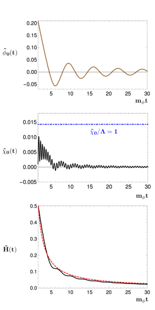
Figure 1: This figure gives the evolution of the background fields and Hubble parameter, where tildes imply we have normalized these quantities by $\sqrt{8\pi}m_{\mbox{\tiny pl}}$, and time is in units of the inflaton mass. For this realization we take $m_{\chi}/m_{\phi}=10$, $m_{\rm pl}/\Lambda=14$ and initial conditions $\phi_{{}_{0}}=1.038~{}m_{\rm pl}$, $\dot{\phi}_{{}_{0}}=-0.662~{}m_{\rm pl}$, $\chi_{{}_{0}}=\dot{\chi}_{{}_{0}}=0.005\;m_{\rm pl}$. The top panel gives the evolution of the inflaton. In the middle panel the solid black curve is $\tilde{\chi}_{{}_{0}}(t)$ and below the dot-dashed blue horizontal line marks the region where the EFT of the background is valid. The bottom plot gives the Hubble rate where the red-dashed line represents a strictly matter dominated evolution.

We begin by studying the behavior of the background fields $\phi_{{}_{0}}$ and $\chi_{{}_{0}}$. These are described by the following equations of motion,

$$\ddot{\phi}_{{}_{0}}+3H\dot{\phi}_{{}_{0}}+\partial_{\chi}\left(\ln f\right)\dot{\phi}_{{}_{0}}\dot{\chi}_{{}_{0}}+f^{-1}\partial_{\phi}V=0,$$ (17)

and

$$\ddot{\chi}_{{}_{0}}+3H\dot{\chi}_{{}_{0}}-\frac{1}{2}(\partial_{\chi}f)~{}\dot{\phi}_{{}_{0}}^{2}+\partial_{\chi}U=0.$$ (18)

If we further assume that the zero-mode dominates the energy density (and pressure) of the universe in the linear regime, then we can write down the evolution equations for the scale factor,

$$H^{2}=\frac{1}{3m_{\rm pl}^{2}}\left(\frac{1}{2}f\dot{\phi}_{{}_{0}}^{2}+\frac{1}{2}\dot{\chi}_{{}_{0}}^{2}+V(\phi_{{}_{0}})+U(\chi_{{}_{0}})\right),$$ (19)

and the Hubble parameter,

$$\dot{H}=-\frac{1}{2m_{\rm pl}^{2}}\left(f\dot{\phi}_{{}_{0}}^{2}+\dot{\chi}_{{}_{0}}^{2}\right).$$ (20)

The first question that we need to address is whether the zero-mode of the reheat field acquires a significant displacement from zero. Using (11), and taking $c_{3}$ and $c_{4}$ to be order-one constants then (18) becomes

$$\ddot{\chi}_{{}_{0}} + 3H\dot{\chi}_{{}_{0}}+\partial_{\chi}U-\frac{\dot{\phi}_{{}_{0}}^{2}}{\Lambda^{2}}\chi_{{}_{0}}-\frac{\dot{\phi}_{{}_{0}}^{2}}{\Lambda}=0,$$ (21)

The last two terms in (21) come from the EFT expansion – i.e. we have dropped terms in the Lagrangian of order $\sim\dot{\phi}_{{}_{0}}^{2}\chi_{{}_{0}}^{3}/\Lambda^{3}$ and higher. Therefore, if either of these terms become large (e.g. if $\chi_{{}_{0}}/\Lambda>1$) then the EFT expansion of the background is not justified. Equation (21) is that of a harmonic oscillator with time-dependent frequency, where the last term resembles an external force, which we also require to be small compared to the restoring force from the effective potential. Assuming that $U(\chi_{{}_{0}})\approx m_{\chi}^{2}\chi_{{}_{0}}^{2}/2$, which is self consistent with our small-displacement assumption, we can find the stable minimum of the effective potential,

$$U_{\rm eff}=U(\chi_{{}_{0}})-\frac{1}{2}\dot{\phi}_{{}_{0}}^{2}f\left(\frac{\chi}{\Lambda}\right).$$ (22)

to be

$$\chi_{{}_{0}}(t)\simeq\frac{\dot{\phi}_{{}_{0}}^{2}}{m_{\chi}^{2}\Lambda}+{\cal O}\left(\frac{\dot{\phi}_{{}_{0}}^{4}}{m_{\chi}^{4}\Lambda^{2}}\right).$$ (23)

The velocity of the inflaton at the end of inflation is roughly $\dot{\phi}\sim m_{\phi}m_{\rm pl}$, which allows us to write down an approximate condition on the size of $\chi_{{}_{0}}$,

$$\frac{\chi_{{}_{0}}}{\Lambda}<1$$ (24)

implies that

$$\frac{m_{\phi}^{2}}{m_{\chi}^{2}}<\left(\frac{\Lambda}{m_{\rm pl}}\right)^{2}$$ (25)

That is, we find that we are free to lower the cutoff of the EFT below the Planck scale ($\Lambda\ll m_{\rm pl}$), but at the cost of increasing the mass of the reheat field above that of the inflaton. The fact that particle production is still possible in the $m_{\chi}\gg m_{\phi}$ regime emphasizes the importance of preheating versus reheating, since in this situation perturbative decays are kinematically forbidden. It is also interesting that this condition is independently required so that the reheat field does not interfere with the the inflationary dynamics prior to reheating (constraints from non-Gaussianity could also be imposed). That is, even for $m_{\phi}<m_{\chi}\simeq 3H_{I}$ such heavy fields can have a dramatic impact on inflation Chen:2009zp ; Cremonini:2010ua ; Achucarro:2010da ; Tolley:2009fg ; Shiu:2011qw ; Avgoustidis:2012yc ; Burgess:2012dz ; Baumann:2011su . We also note that the presence of a discrete $Z_{2}$ symmetry could be used to forbid the dimension five operator leading to the tadpole in (21), and our stability condition (25) would still hold due to the presence of the dimension six operator.

We have numerically verified the result (25) by solving the system (17)-(19) for a range of masses, initial conditions, and the cutoff $\Lambda$. In Figure 1, we plot a particular realization of a consistent configuration for the background fields together with the evolution of the cosmological background. In the plot, we take $m_{\rm pl}/\Lambda=14$ and $m_{\chi}/m_{\phi}=10$ consistent with (25). We see that the background value $\chi_{{}_{0}}$ stays consistent within the EFT regime, while inflaton oscillations proceed as in the case of a quadratic potential. On the other hand, it can be seen that the expansion of the universe is slightly faster than $H(t)\propto t^{-1}$ initially, and then asymptotes to this behavior at late times $m_{\phi}t\gg 1$. We conclude this section by emphasizing that in order to have a stable, well-behaved background solution within the regime of validity of the EFT, one requires the condition, (25) to be satisfied.

III.2.1 Non-perturbative Dynamics and Limitations of the Background EFT

We now consider whether resonant particle production is possible around the background we analyzed in the previous section. Expanding both scalar fields to first order around their background values, $\phi=\phi_{{}_{0}}+\delta\phi$, $\chi=\chi_{{}_{0}}+\delta\chi$ in the Lagrangian (10), we write the equation of motion for the linearized fluctuations of the reheat field in Fourier space as

$$\delta\ddot{\chi}_{k}+3H\delta\dot{\chi}_{k}+\left[\left(\frac{k}{a}\right)^{2}+m_{\chi}^{2}-\frac{\dot{\phi}_{{}_{0}}^{2}}{\Lambda^{2}}\right]\delta\chi_{k}=2\frac{\dot{\phi}_{{}_{0}}}{\Lambda}\left[1+\frac{\chi_{{}_{0}}}{\Lambda}\right]\delta\dot{\phi}_{k},$$ (26)

where the terms on the right side are due to the mixing with inflaton fluctuations. These terms can source $\delta\chi_{k}$ fluctuations whenever $\delta\dot{\phi}_{k}$ is large. In the initial stage of (p)reheating the effect of this term will be negligible. Neglecting these terms, we focus on sub-Hubble scales first neglecting the cosmological expansion (we take $a(t)\to 1$, $H(t)\to 0$). In this approximation, (26) becomes

$$\delta\ddot{\chi}_{k}+\left[k^{2}+m_{\chi}^{2}-\frac{\dot{\phi}_{{}_{0}}^{2}}{\Lambda^{2}}\right]\delta\chi_{k}=0,$$ (27)

where we define the frequency of the modes as $\omega_{k}^{2}(t)=k^{2}+m_{\chi}^{2}-\dot{\phi}_{{}_{0}}^{2}/\Lambda^{2}$. Given a coherently oscillating inflaton, $\phi_{{}_{0}}=\Phi(t)\sin(m_{\phi}t)$, we can map this mode equation to the Mathieu equation

$$\delta{\chi}_{k}^{\prime\prime}+\left[A_{k}-2q\cos(2z)\right]\delta\chi_{k}=0,$$ (28)

where we have defined the dimensionless time $z=m_{\phi}t$ and $A_{k}=(k^{2}+m_{\chi}^{2})/m_{\phi}^{2}-2q$ with $q=\Phi^{2}/4\Lambda^{2}$. Floquet’s theorem VogtNilsen:1956mr states that for a given wave-number, (26) has solutions of the form

$$\delta\chi_{k}=e^{\mu_{k}z}g_{1}(z)+e^{-\mu_{k}z}g_{2}(z),$$ (29)

where $g_{1}$ and $g_{2}$ are periodic functions and $\mu_{k}$ is the Floquet exponent. In general, the Floquet exponent $\mu_{k}$ depends on the wave number $k$, the mass of the reheat field $m_{\chi}$, and the ratio $\Phi/\Lambda$. For cases where the real part of the exponent is non-zero, we have exponentially growing modes of $\delta\chi_{k}$.

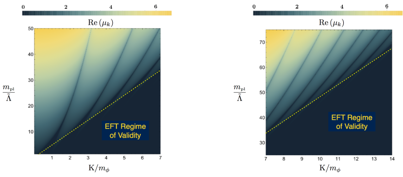
Figure 2: Instability band structure for the model $V_{\rm tot}=\frac{1}{2}m_{\phi}^{2}\phi^{2}+\frac{1}{2}m_{\chi}^{2}\chi^{2}-\frac{1}{2}\dot{\phi}_{{}_{0}}^{2}f\left(\frac{\chi}{\Lambda}\right)$, where $f$ is given by (11). This density plot represents the real part of the scaled Floquet exponent, $\mbox{Re}(\mu_{k})$, where lighter regions represent larger values. The y-axis is the hierarchy between the Planck mass and the rescaled cut-off of the EFT, $\tilde{\Lambda}=\Lambda/\sqrt{8\pi}$, while the x-axis corresponds to $K=\sqrt{k^{2}+m_{\chi}^{2}}$ in units of $m_{\phi}$.

The structure of (28) tells us that the resonant momenta are grouped into bands in parameter space. Since $k^{2}>0$, and hence, $A_{k}>-2q$, there are also meaningful statements one can make about the regions of the Mathieu parameter space that are probed by our reheating models. One interesting case is when some modes satisfy $-2q<A_{k}<0$; in this case, (28) assures us that there’s a time when the mass-squared of the these modes is negative (analogous to the cases explored in Greene:1997ge ) and the Floquet exponent can be very large, $\mu_{k}\simeq(4/\pi)~{}q^{1/2}$ for $q\gg 1$. There’s another case in which $0<A_{k}<2q$, where the mass-squared of some of the $\delta\chi_{k}$ modes become tachyonic for certain time intervals and is also very efficient (analogous to Felder:2000hj .)

On the other hand, $A_{k}$ is frequently larger than $2q$. While these models have parametric instabilities, the resonance structure requires us to be more careful. For our purposes here, the consistency of the background EFT requires the mass of the reheat field to satisfy $m_{\chi}^{2}>\dot{\phi}_{{}_{0}}^{2}/\Lambda^{2}$, which requires avoiding the regions of the parameter space that guarantee strong, broad, resonance. While the inflaton undergoes periodic oscillations this condition implies

$$m_{\chi}^{2}>m_{\phi}^{2}\frac{\Phi^{2}}{\Lambda^{2}},$$ (30)

which is exactly what we have found in equation (25) with $\Phi=m_{\rm pl}$. Here, we have used $\phi(t)=\Phi\sin(m_{\phi}t)$ considering the maximum value of $\dot{\phi}_{{}_{0}}^{2}/\Lambda^{2}$. We have also studied this system numerically, using FloqEx floqex , with our results appearing in Figure 2. The figure shows the magnitude of the Floquet exponent as a function of cutoff and wave number. One can see the broad (and tachyonic) resonance regimes mostly live outside of those probed by the EFT. We must keep in mind, though, that these estimates could still produce some particles through parametric resonance, and should be studied through full lattice methods – we leave this to future work.

Our main conclusion thus far is that if we require the reheat field to respect the shift symmetry of the inflationary sector (implying adequate inflation consistent with CMB observations), successful reheating suggests considering an EFT cutoff far below the Planck scale $\Lambda\ll m_{\rm pl}$. We saw that having such a sub-Planckian cutoff can quickly lead to the breakdown of the background EFT expansion when we require efficient reheating in the EFT.

As another example of when the EFT expansion may breakdown, consider the corrections we have thus far neglected in (7). When evaluated on the background the operator contains a term

$$\frac{c_{1}}{\Lambda^{4}}\left(\partial\phi\right)^{4}\supset\frac{c_{1}}{\Lambda^{4}}\dot{\phi}_{0}^{2}\left(\partial\phi\right)^{2}.$$ (31)

During inflation this term will be slow-roll suppressed $\dot{\phi}_{0}^{2}/\Lambda^{4}\sim\epsilon\,H^{2}m_{\rm pl}^{2}/\Lambda^{4}$ and higher order terms will be even further suppressed as long as $\Lambda$ is not far below $m_{\rm pl}$ during inflation. However, for smaller values of the cutoff this corresponds to strong coupling of the background and our EFT approach breaks down – this would also lead to a large level of non-Gaussianity Baumann:2011su . Assuming the background remains weakly coupled at the end of inflation we have

$$\frac{c_{1}}{\Lambda^{4}}\dot{\phi}_{0}^{2}\sim\frac{m_{\phi}^{2}\phi_{e}^{2}}{\Lambda^{4}}\sim\left(\frac{m_{\phi}}{m_{\rm pl}}\right)^{2}\left(\frac{\phi_{e}}{m_{\rm pl}}\right)^{2}\left(\frac{m_{\rm pl}}{\Lambda}\right)^{4},$$ (32)

so for $\Lambda$ far below the Planck scale the EFT would again fail as this term would be as important as the kinetic term (and terms even higher in derivatives that we neglected would also be important). For example, in chaotic inflation where the inflaton mass is fixed by the COBE normalization this implies $\Lambda\gtrsim 10^{-3}\,m_{\rm pl}$. We emphasize that this constraint has nothing to do with requiring adequate inflation and is an added constraint for the consistency of the derivative expansion of the EFT during reheating. We now turn to a different EFT approach where the challenges discussed in this section can be addressed.

IV The EFT of (p)Reheating

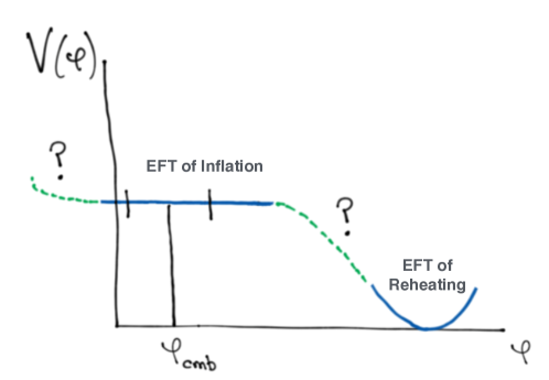
Figure 3: Obtaining adequate inflation, ending inflation and then successful reheating in the EFT requires a complete knowledge of the inflationary potential. This presents a challenge when using Weinberg’s EFT approach to capture reheating in many classes of models.

We have seen that using an EFT approach to the background has limited utility in simultaneously describing inflation and reheating. Indeed, in addition to the challenges discussed at the end of Section III, an additional concern is that there could be terms that badly break the shift symmetry at the time of reheating. Such terms could be small during inflation (suppressed by the breaking scale), but could be important at the time of reheating. Alternatively, there are many reheating models in which the shape of the potential during inflation is vastly different than it is during reheating (and could include additional fields like in hybrid models) and the background EFT approach requires a knowledge of the complete potential. This is illustrated in Figure 3.

In particular, the terms arising from the breaking of the shift symmetry of the inflaton (which would include thus far forbidden terms of the form $g_{i}\phi^{p}\chi^{q}$) could become as important as the other terms we have considered in (26). As another example consider the potential

$$V=\frac{m^{2}M^{2}}{2\alpha}\left[\left(1+\frac{\phi^{2}}{M^{2}}\right)^{\alpha}-1\right].$$ (33)

where $\alpha<1$. This toy model captures many important inflationary models including axion monodromy Amin:2011hj . During the inflationary phase this potential scales as $V\sim\phi^{2\alpha}$ and is sensitive to the scale $M$, whereas the behavior during reheating ($\phi<M$) is independent of $M$ and $V\sim m^{2}\phi^{2}$. So in our EFT approach expanding the field in powers of $\phi/\Lambda$ is causing us to miss these types of theories.

In addition, new degrees of freedom could appear at the time of reheating that were heavy during inflation and could have been integrated out – in other words the EFT during inflation and the EFT during reheating can correspond to two distinct EFTs. This is not to say our approach doesn’t capture many models. In particular, we’ve seen that the model of ArmendarizPicon:2007iv is captured by our approach, and most chaotic inflation models would be as well. But even focusing only on the inflationary epoch we know that Weinberg’s EFT is not capable of capturing a large number of interesting models. For example, in DBI type models where the background is in some sense strongly coupled one needs a non-perturbative expression for the background as it is a resummed expression where each derivative in the derivative expansion must be kept, e.g. $V\sim\sqrt{1-\dot{\phi}^{2}/\Lambda^{4}}$. Such models are not captured by the Lagrangian of (7). One may also anticipate reheating models where the background of the reheat field could also exhibit such non-linear behavior and then the derivative expansion of the Lagrangian (8) would be inadequate – as well as the expansion of the mixing terms stopping at dimension six in (9). One final objection is that we have only concentrated on scalar reheat fields. Reheating to fermions and gauge fields is also important, and the way in which this proceeds is not only model dependent, but the spin statistics can also make important differences in the efficiency of reheating Adshead:2016xxj .

Given these shortcomings of the EFT of the background we now turn to construct an EFT for reheating along the lines of the EFT of Inflation Cheung:2007st . As we will discuss, this approach can overcome many of the obstacles established in this Section. In the remainder of this section, we first begin by constructing an EFT focusing on the fluctuations directly at the end of inflation. This theory will share many similarities with the EFT of multi-field inflation Baumann:2011su ; Senatore:2010wk . However there will be important differences which we will discuss. We then demonstrate how the approach can reproduce both the results of self resonant reheating and multi-field reheating. We also discuss some new models that arise from considering the symmetries of the EFT.

IV.1 Construction of the EFT of Fluctuations

The EFT expansion in fluctuations (rather than the background) relies on the fact that the background expansion of the universe spontaneously breaks time-translation invariance. Over the history of the universe there have been many different dominant forms of matter and energy, and so many different sources of time-translation breaking including; inflatons, post-inflation / pre-BBN fields, radiation, dark matter, and eventually dark energy today. As the universe passed through these phases the energy density changed its composition many times, but the scale factor continued to monotonically increase. The EFT approach takes this background evolution as given a priori (as specified by the background functions $a(t)$, $H(t)$, and $\dot{H}(t)$) and focuses directly on the most general EFT for the fluctuations around this background.

In taking this approach we give up on realizing explicit models for the background, and instead focus on implications and observations associated with the fluctuations. In regards to connecting with observations this approach is adequate, since physical observables correspond to fluctuations and not background quantities Cheung:2007sv . The approach also has the advantage that the underlying physics responsible for driving the background expansion can be non-perturbative, in the sense that the background doesn’t need to admit an EFT expansion (as we required in Section III). Instead, this EFT approach is more general and models are classified by their symmetry breaking properties and the allowed operators in the Lagrangian correspond to cosmological perturbations. In many cases the symmetries alone can be used to establish rigid constraints on the theory of the fluctuations and associated observables. For example, it is well known that inflation requires that de Sitter symmetry must be non-linearly realized and this leads to constraints on inflaton correlation functions. This fact is manifest in the EFT of Inflation approach using the corresponding Goldstone boson Cheung:2007sv . This EFT approach has also been shown to be useful when the cosmological background changes its behavior, e.g. in the EFT of dark energy Gubitosi:2012hu ; Bloomfield:2012ff ; Fasiello:2016qpn ; Fasiello:2016yvr ; Lewandowski:2016yce , where one is primarily interested in observations during matter domination, but also must account for observations during dark energy domination.

The generality of the EFT approach when applied to cosmological backgrounds was first established in Creminelli:2006xe , where the authors were investigating violations of the Null Energy Condition in non-standard cosmologies. In that paper, referencing earlier work of Weinberg Weinberg:2003sw , it was pointed out that on long wavelengths there is always an adiabatic mode corresponding to the Goldstone boson of spontaneously broken time diffeomorphism invariance. Whenever a decoupling limit exists – in which the Goldstone decouples from gravity – this broken symmetry is then realized as spontaneously broken time translation invariance (the gauge symmetry effectively becomes a global symmetry). Thus, for any FRW spacetime it is possible to utilize the EFT approach and it is in this vain that we will construct our EFT for reheating following the initial ideas presented in Ozsoy:2015rna .

As an example, suitable for studying the dynamics at the end of inflation, we can consider a decelerated FRW expansion with the background metric

$$ds^{2}=-dt^{2}+a^{2}(t)\delta_{ij}dx^{i}dx^{j},~{}~{}~{}\ddot{a}(t)<0.$$ (34)

We can think of this background as generated by the evolution of a set of homogeneous scalars fields, i.e. $\{\phi_{{}_{0}},\chi_{{}_{0}},\dots\}$. In this work, to study dynamics at the end of inflation, we may consider only one of the scalars, e.g. the inflaton $\phi_{{}_{0}}$, that contributes significantly to the evolution of scale factor, $a(t)$. This FRW evolution has a preferred time slicing described by the homogeneous scalar which can also be considered a clock. In order to describe the theory of fluctuations around this background, we can go to a co-moving frame (unitary gauge) where the vacuum expectation value of the scalar coincides with this privileged time slicing, corresponding to distinct values of $\langle\phi\rangle=\phi_{{}_{0}}$. As we have fixed the slicing of space-time, general time diffs are no longer a symmetry and the fluctuations of the scalar are hidden in the metric perturbations, which now describe three degrees of freedom: two transverse for the graviton and one for the scalar. We can always re-introduce inflaton fluctuations by a common local shift in time, i.e. $t\to t+\pi(x)$. By definition, such a fluctuation corresponds to an adiabatic fluctuation, proportional to Goldstone mode $\delta\phi=\dot{\phi}_{{}_{0}}\pi$ associated with the broken symmetry. In this work, apart from the adiabatic fluctuations, we will consider an additional degree of freedom $X(t,x)=\chi_{{}_{0}}(t)+\chi(t,x)$, which will play the role of the (p)reheat field. As is standard in the literature we will take this field to be a subdominant source of background evolution during the first stages of preheating (i.e. $\rho_{\phi}\gg\rho_{\chi}$) since before particle creation $\langle X\rangle\simeq 0$.

IV.1.1 The Action in Unitary Gauge

The procedure for constructing the EFT of fluctuations for the inflationary sector coupled to a reheat field at the time of reheating is similar to the case of quasi-single field inflation considered in Noumi:2012vr . Those authors considered the effects of particle production during inflation, whereas here we consider reheating and important differences will be discussed below. Nevertheless, the action can be constructed analogously and working in unitary gauge the action for the fluctuations is

$$S=\int d^{4}x\sqrt{-g}\left[\frac{m_{\rm pl}^{2}}{2}R-f_{1}(t)-f_{2}(t)g^{00}+F^{(2)}(\delta g^{00},\chi,\delta R_{\mu\nu\rho\sigma},\delta K_{\mu\nu};\nabla_{\mu};t)\right],$$ (35)

where $f_{1}$ and $f_{2}$ are arbitrary functions of time, $F^{(2)}$ starts quadratic in operators which must be covariant in spatial indices but not in time, $\nabla_{\mu}$ is the covariant derivative, and $\delta R_{\mu\nu\rho\sigma}$ and $\delta K_{\mu\nu}$ are the fluctuations in the Riemann tensor and extrinsic curvature, respectively. Note that the second and third terms in the above action are the only ones that contain linear perturbations. Requiring that terms linear in the fluctuations vanish (i.e. tadpole cancelation) follows from enforcing the background equations of motion in an FRW background Cheung:2007st ,

$$3H^{2}m_{\rm pl}^{2}=f_{1}(t)+f_{2}(t),$$ (36)

and

$$-2\dot{H}m_{\rm pl}^{2}=2f_{2}(t).$$ (37)

As a simple example of tadpole cancelation, consider the end of inflation where the inflaton begins oscillating with a potential $V(\phi)$ and where derivative interactions and the density of other fields are negligible. In this case the functions in (37) are given by $f_{1}=V(\phi_{{}_{0}})$ and $f_{2}=\dot{\phi}_{{}_{0}}^{2}/2$. However, more generally, $f_{1}$ and $f_{2}$ can take any form as long as the background corresponds to the (p)reheating period, i.e. an FRW universe with possibly small corrections due to oscillations. For example, we could have a preheating model corresponding to DBI-like models of inflation where a large number of derivative self-interactions could play an important role Child:2013ria . In that case the functions $f_{1}$ and $f_{2}$ would contain terms with an infinite number of derivatives at the level of the background. The key is that the behavior of the matter sector will be captured by the functions $f_{1}$ and $f_{2}$, and once we cancel the tadpoles, the background is then given (by the equations of motion) by $H(t)$ and its derivatives. Then, we can focus on the EFT of the fluctuations about this background – just as in the case of the EFT of Inflation or DE Cheung:2007st ; Bloomfield:2012ff ; Gubitosi:2012hu . Thus, the problem we encountered in the previous section, where we would need to keep all the terms in the $\chi/\Lambda$ expansion is not an issue here. Instead, these terms are captured by $H$ and $\dot{H}$ and could represent re-summed, non-perturbative expressions for the background. Moreover, because we are not performing a perturbative expansion of the background, we work under the assumption that we have a complete knowledge of the potential overcoming the problems associated with Figure 3.

The most general action is found by expanding the function $F^{(2)}$ in (35) in terms of fluctuations $\{\delta g^{00},\chi,\delta K_{\mu\nu},\delta R_{\mu\nu\rho\sigma}\}$ and their derivatives. We emphasize that this EFT expansion is one in perturbations and derivatives. During reheating, the fluctuations are also assumed to be initially small, however significant particle production can change this (as we will discuss). Whereas the derivative expansion follows from locality, causality and unitarity in an FRW universe. In the gravity sector, $\delta g^{00}$ is a zero derivative object, whereas $\delta K_{\mu\nu}$ corresponds to one derivative and $\delta R_{\mu\nu\rho\sigma}$ to two, as they contain first and second order derivatives of the metric, respectively. When we introduce the Goldstone boson in the next section, it will be clear that terms with $\delta K$ and $\delta R$ will include higher derivatives of the Goldstone boson. Finally, we find it convenient to split the action in (35) into three parts

$$S=S_{\rm g}+S_{\chi}+S_{\rm g\chi},$$ (38)

where the action $S_{\rm g}$ contains only terms build out of $\{\delta g^{00},\delta K_{\mu\nu},\delta R_{\mu\nu\rho\sigma}\}$, $S_{\chi}$ contains those purely from $\chi$ and the action $S_{\rm g\chi}$ is due to mixing between gravity sector and $\chi$. Following our discussion above, we then have

$$S_{\rm g}=\int d^{4}x\sqrt{-g}\left[\frac{m_{\rm pl}^{2}}{2}R-m_{\rm pl}^{2}\left(3H^{2}(t)+\dot{H}(t)\right)+m_{\rm pl}^{2}\dot{H}(t)g^{00}+\frac{m_{2}^{4}(t)}{2!}\left(\delta g^{00}\right)^{2}+\ldots\right],$$ (39)

$$S_{\chi}=\int d^{4}x\sqrt{-g}\left[-\frac{\alpha_{1}(t)}{2}g^{\mu\nu}\partial_{\mu}\chi\partial_{\nu}\chi+\frac{\alpha_{2}(t)}{2}(\partial^{0}\chi)^{2}-\frac{\alpha_{3}(t)}{2}\chi^{2}+\alpha_{4}(t)\chi\partial^{0}\chi\right],\;\;$$ (40)

$$S_{{\rm g}\chi}=\int d^{4}x\sqrt{-g}\left[\beta_{1}(t)\delta g^{00}\chi+\beta_{2}(t)\delta g^{00}\partial^{0}\chi+\beta_{3}(t)\partial^{0}\chi-(\dot{{\beta}}_{3}(t)+3H(t)\beta_{3}(t))\chi\right],$$ (41)

where $g^{00}=-1+\delta g^{00}$ and the dots represent terms higher order in fluctuations and derivatives. Here, $\{m_{2}(t),\alpha_{i}(t),\beta_{i}(t)\}$ are thus far arbitrary functions of time that are permitted in the unitary gauge as time diffs have been spontaneously broken by the background. We note that the coefficient of the $\delta g^{00}$ operator is fixed by the background, implying that it is universal in the sense that all preheating models with the same background evolution will have the same coefficient (specified by $H(t)$ and its derivatives). Whereas, the operator $\left(\delta g^{00}\right)^{2}$ is an example of a non-universal operator, because $m_{2}$ is not fixed by the symmetries of the FRW background. Instead its value corresponds to a specific class of models (those with a non-unity sound speed). Similarly, broken time diffs generally allow for a term proportional to $\alpha_{2}$ that leads to non-trivial sound speed $c_{\chi}=\alpha_{1}/(\alpha_{1}+\alpha_{2})$ in the reheat sector $\chi$. In (41), the functions $\beta_{i}$ can be seen as a measure of the strength of mixing with gravitational fluctuations (including one scalar d.o.f). At this stage, the usefulness of this approach might be in question, given the large number of free parameters. However, as we will see in the following sections, even though this is the most general theory to quadratic order, in practice many of the terms in (39)-(41) are not important for elementary processes within reheating. Finally, we can further simplify the action by performing a field re-definition of $\chi$, using that $\chi=0$ on the background trajectory and using time reparametrization invariance to set $\alpha_{4}=\beta_{3}=0$ in the actions (40) and (41).

The form of (39), (40) and (41) are not particularly useful in studying the dynamics as the scalar fluctuation representing inflaton is not manifest. We can re-introduce diffeomorphism invariance and the Goldstone mode related to inflaton by the Stückelberg trick, which will be our main focus in the following section.

IV.1.2 Introducing the Goldstone Boson

To introduce the Goldstone boson along with time diffs, we first perform the broken time diffs $t\rightarrow t+\xi^{0}(t,\vec{x})$ in the actions (39)-(41). Since the cosmological background (i.e. $H,\dot{H}$) as well as the free functions $\{\alpha_{i},\beta_{i}\}$ depend on cosmic time, $t$. The gauge function, $\xi^{0}$, will appear explicitly in the actions for the perturbations. We then replace $\xi^{0}\rightarrow\pi(t,\vec{x})$ everywhere it appears in the action and require that the Goldstone transforms non-linearly, $\pi\rightarrow\pi-\xi^{0}$ under diffs. In this way, clearly full diffeomorphism invariance can be restored in (39)-(41). In order to find the explicit form of the actions including the Goldstone $\pi$, we need to know the transformation rule for the remaining operators appearing in (39)-(41) under $t\to t+\pi$. Under the transformation we have

$$g^{00} \rightarrow g^{00}+2g^{0\mu}\partial_{\mu}\pi+g^{\mu\nu}\partial_{\mu}\pi\partial_{\nu}\pi,$$

$$g^{i0} \rightarrow g^{i0}+g^{i\nu}\partial_{\nu}\pi,$$

$$\partial^{0}\chi \rightarrow \partial^{0}\chi+g^{\mu\nu}\partial_{\mu}\chi\partial_{\nu}\pi,$$

$$f(t) \rightarrow f(t+\pi)$$ (42)

$$R_{\mu\nu\lambda\sigma} \rightarrow R_{\mu\nu\lambda\sigma}$$ (43)

$$\int d^{4}x\sqrt{-g} \rightarrow \int d^{4}x\sqrt{-g}$$

where $f(t)$ represents any time-dependent function appearing in the action. Carrying out this procedure on the action (39) we find

$$S_{\rm g} =\int d^{4}x\sqrt{-g}\Bigg{[}\frac{m_{\rm pl}^{2}}{2}R-m_{\rm pl}^{2}\left(3H(t+\pi)^{2}+\dot{H}(t+\pi)\right)$$

$$~{}~{}~{}~{}~{}~{}~{}~{}~{}~{}~{}~{}~{}~{}~{}~{}~{}~{}~{}~{}+m_{\rm pl}^{2}\dot{H}(t+\pi)(g^{00}+2g^{0\mu}\partial_{\mu}\pi+g^{\mu\nu}\partial_{\mu}\pi\partial_{\nu}\pi)$$

$$~{}~{}~{}~{}~{}~{}~{}~{}~{}~{}~{}~{}~{}~{}~{}~{}~{}~{}~{}~{}+\frac{m_{2}^{4}(t+\pi)}{2!}(\delta g^{00}+2g^{0\mu}\partial_{\mu}\pi+g^{\mu\nu}\partial_{\mu}\pi\partial_{\nu}\pi)^{2}\Bigg{]}\ .$$ (44)

We see that this action is invariant under time diffs if we require the Goldstone to transform as $\pi\rightarrow\pi-\xi^{0}({t,\vec{x}})$, i.e. the symmetry is non-linearly realized Senatore:2010wk . We also note that requiring the symmetry be realized in the UV has forced relationships between the various operators (all the terms in parentheses must have the same coefficients). Following the same steps, (40) and (41) become

$$S_{\chi} =\int d^{4}x\sqrt{-g}\left[-\frac{\alpha_{1}(t+\pi)}{2}g^{\mu\nu}\partial_{\mu}\chi\partial_{\nu}\chi+\frac{\alpha_{2}(t+\pi)}{2}(\partial^{0}\chi+\partial_{\mu}\pi\partial^{\mu}\chi)^{2}\right.$$

$$\left.~{}~{}~{}~{}~{}~{}~{}~{}~{}~{}~{}~{}~{}~{}~{}~{}~{}~{}~{}-\frac{\alpha_{3}(t+\pi)}{2}\chi^{2}\right],$$ (45)

$$S_{{\rm g}\chi} =\int d^{4}x\sqrt{-g}\Big{[}\beta_{1}(t+\pi)(\delta g^{00}+2\partial^{0}\pi+\partial_{\mu}\pi\partial^{\mu}\pi)\chi$$

$$~{}~{}~{}~{}~{}~{}~{}~{}~{}~{}~{}~{}~{}~{}~{}+\beta_{2}(t+\pi)(\delta g^{00}+2\partial^{0}\pi+\partial_{\mu}\pi\partial^{\mu}\pi)(\partial^{0}\chi+\partial_{\mu}\pi\partial^{\mu}\chi)\Big{]}.$$ (46)

Similar to the discussion above, the non-linearly realized symmetry introduces interactions between $\chi$ and the Goldstone, $\pi$.

To describe the dynamics at the end of inflation, working with the full action given by $S_{\rm g}+S_{\chi}+S_{\rm g\chi}$ in complete generality is a difficult task. First of all, we need to have some input for the time-dependent functions, i.e. $\{H(t),\alpha_{i}(t),\beta_{i}(t)\}$ appearing in the Lagrangian. However, as we will see, an investigation on the background dynamics during reheating along with the associated symmetries and scales of interest will allow us to obtain generic information on the form of these functions. This will be our main focus in the next section.

IV.2 Background Evolution During Reheating and Symmetries of the Action

IV.2.1 Background Evolution and Symmetries

In parametrizing the background expansion we have assumed a decelerating FRW universe. A simple example is provided by a perfect fluid with an equation of state $w$ and with corresponding scale factor $a(t)\propto t^{2/3(1+w)}$ and expansion rate $H(t)=\dot{a}/a\propto t^{-1}$ with $H^{-1}$ setting the cosmic time scale. On the other hand, in studies of the dynamics at the end of inflation the frequency of inflaton oscillations introduce another important time scale. For example, if the inflaton oscillates in a power-law potential, $V\propto\phi_{{}_{0}}^{n}$, the period of oscillations will be $2\pi\omega^{-1}=4\int_{0}^{\phi_{i}}{\rm d}\phi_{{}_{0}}~{}(V(\phi_{i})-V(\phi_{{}_{0}}))^{-1/2}$, which for general $n$ depends on the initial amplitude, $\phi_{i}$ Johnson:2008se . In the limit that the period of oscillations is much smaller than the expansion time scale, $\omega^{-1}\ll H^{-1}$, coherent scalar field oscillations behave like a perfect fluid with an average equation of state, $\langle w\rangle_{\rm a}=(n-2)/n+2$ Turner:1983he .

The presence of two different time scales leads to interesting symmetry breaking patterns within the EFT, and whether a symmetry is realized will depend on the dynamics under investigation. At high energies (or small wavelengths) the energy being probed $E_{\rm{probed}}$ exceeds both the oscillation and expansion energy i.e. $E_{\rm{probed}}\gg\omega\gg H$ and so the time evolution of the oscillator and the cosmic expansion is negligible – time-translations are a good symmetry. As we lower the energy scale to $E_{\rm{probed}}\lesssim\omega$ we first break time-translation invariance down to a discrete symmetry $t\to t+2\pi\omega^{-1}$. Then as we further lower the energy to $E_{\rm{probed}}\lesssim H\ll\omega$ this discrete symmetry is further broken by the cosmic expansion. This symmetry breaking reflects that on large scales (low-energy) we have an expanding universe, but on sub-Hubble scales the only time dependence results from the oscillating scalar field and the effect of the expansion can be ignored. And at even higher energies (smaller distances / faster time scales) the scalar oscillations would not be probed.

This hierarchy in scales can be captured by parameterizing the background behavior by a Hubble rate that is a sum of a monotonically evolving part and a small rapidly oscillating component,

$$H(t)=H_{{\mbox{\tiny FRW}}}(t)+H_{\rm osc}(t)P(\omega t),$$ (47)

where the first term is adiabatically evolving $H_{{\mbox{\tiny FRW}}}(t)\propto t^{-1}$ and monotonically decreasing, whereas the second term leads to an oscillatory correction described by a general periodic function $P(\omega t)$ with period $T=2\pi\omega^{-1}$. In order to ensure an overall monotonic FRW evolution we take the first term to be dominant, $H_{{\mbox{\tiny FRW}}}\gg H_{\rm osc}$. This implies our clock is always monotonically increasing – as exemplified by the monotonic evolution of the scale factor $a(t)$ in an FRW universe. This situation is to be contrasted with models where the universe itself is oscillating Bains:2015gpv , which can exhibit a number of pathologies Easson:2016klq . We also note that the time dependence of $H_{{\mbox{\tiny FRW}}}$ and $H_{\rm osc}$ is slow compared with the time scale of oscillations $\omega^{-1}$, i.e. $\dot{H}_{{\mbox{\tiny FRW}}}/(H_{{\mbox{\tiny FRW}}}\omega)\sim\dot{H}_{\rm osc}/(H_{\rm osc}\omega)\ll 1$. This corresponds to our earlier statement that on short time scales (larger energies) there is an approximate discrete symmetry.

An important question is whether we can generalize the symmetry arguments above for the time-dependent functions associated with the non-universal operators in (IV.1.2)-(46), i.e. $\{m_{2},\alpha_{i},\beta_{i}\}$. On general grounds, in an FRW background described by (47) we expect that the functions $m_{2},\alpha_{i},\beta_{i}$ – which describe the self-couplings, and couplings/mixings between the Goldstone and the reheat sector $\chi$ – to be a generic function of the Hubble rate in (47) and its derivatives. Depending on the couplings between these sectors this suggests that in general we can write these functions in the form

$$F_{i}(t)=M^{p}_{i}(t)P^{\prime}(\omega^{\prime}t),$$ (48)

where in general the periodic function $P^{\prime}$ is different from the one in (47) as is the frequency $\omega^{\prime}\neq\omega$. Here, the index $i$ collectively represents time-dependent functions $\{m_{2},\alpha_{i},\beta_{i}\}$ and $p$ denotes the mass dimension of these functions. Suggested by the symmetry breaking pattern we discussed above, we can similarly take $\dot{M}_{i}/(M_{i}\omega)\ll 1$.

IV.2.2 Symmetries of the Action and Implications

An important consequence of the discrete symmetry of the Goldstone is that non-derivative interactions can appear in the action. When this is a good symmetry we can expand the background and non-universal parameters $\{H,\dot{H},m_{2},\alpha_{i},\beta_{i}\}$ in the form

$$F_{i}(t+\pi)=F_{i}(t)+\dot{F}_{i}(t)\pi+\frac{1}{2}\ddot{F}_{i}(t)\pi^{2}+\dots~{}.$$ (49)

This breaking is similar in spirit to the work of Behbahani:2011it , where those authors considered resonant non-Gaussianity induced through small-scale oscillations in $H$ and $\dot{H}$ during single-field inflation. In the two-sector EFT we are considering here we can extend that study to dynamics that arise in the presence of interactions between the Goldstone $\pi$ and reheating $\chi$ sectors. Moreover, contrary to the situation during inflation, where there is a fixed energy scale corresponding to horizon crossing, Cheung:2007st , to study dynamics at the end of inflation we are often interested in the dynamics at sub-Hubble scales. For sub-Hubble scales with $E_{\rm{probe}}>\omega$ we expect interactions induced by expanding the time-dependent functions in (49), which parametrize important contributions to the dynamics. Such interactions can induce large loop corrections for the parameters of the EFT, and additionally back-reaction effects can become large and the perturbative expansion of the EFT of fluctuations will fail. In typical studies of preheating, the importance of such contributions correspond to the end of ‘stage one’, which can be followed by turbulence and chaotic behavior Kofman:1997yn . We leave an investigation of these stages to future work. In the following, we will focus on the first stages of preheating and establish how our framework captures existing models. We will also explore new models and their connection to observations during the first stages of preheating.

IV.3 Capturing Existing Models

IV.3.1 Reheating Through Self-Resonance

In this section, we focus on the Goldstone sector in (IV.1.2) to construct models of reheating through self-resonance. That is, we want to establish how the EFT reproduces self-resonant models of reheating where inflaton ‘particles’ (here corresponding to the Goldstone $\pi\sim\delta\phi$) are created from oscillations of the background condensate $\phi_{{}_{0}}(t)$. We will also consider when gravitational fluctuations can be shown to decouple. To begin we expand the time-dependent functions in (IV.1.2) and use the ADM decomposition of the metric in spatially flat gauge working to second order in fluctuations $\delta N,N^{i}$ and $\pi$. We have

$$\mathcal{L}_{\pi_{c}} = \frac{1}{2}\left(\dot{\pi}_{c}^{2}-c_{\pi}^{2}\frac{(\partial_{i}\pi_{c})^{2}}{a^{2}}\right)-\frac{1}{2}m_{\pi}^{2}(t)\pi_{c}^{2}-\frac{(-2\dot{H})^{1/2}}{c_{\pi}}\left(\dot{\pi}_{c}\delta N_{c}-\frac{1}{2}\left(\frac{\ddot{H}}{\dot{H}}-2\frac{\dot{c}_{\pi}}{c_{\pi}}\right)\pi_{c}\delta N_{c}\right)$$ (50)

$$+ (-2\dot{H})^{1/2}c_{\pi}~{}\left(3H\delta N_{c}+\partial_{i}N^{i}_{c}\right)~{}\pi_{c}+\dots$$

where we introduced the canonical fields $\pi_{c}=\sqrt{-2\dot{H}m_{\rm pl}^{2}}~{}c_{\pi}^{-1}\pi,\,\delta N_{c}=m_{\rm pl}\delta N,N^{i}_{c}=m_{\rm pl}N^{i}$, the sound speed of the fluctuations is $c_{\pi}^{2}=m_{\rm pl}^{2}\dot{H}/(m_{\rm pl}^{2}\dot{H}-m_{2}^{4})$, and we neglect terms involving the scalar curvature as they are sub-leading.

An important consequence of the background evolution and time-dependent sound speed is that it induces a time-dependent mass for the Goldstone

$$m_{\pi}^{2}=-3\dot{H}c_{\pi}^{2}-\frac{1}{4}\left(\frac{\ddot{H}}{\dot{H}}-2\frac{\dot{c}_{\pi}}{c_{\pi}}\right)^{2}-\frac{3H}{2}\left(\frac{\ddot{H}}{\dot{H}}-2\frac{\dot{c}_{\pi}}{c_{\pi}}\right)-\frac{1}{2}\partial_{t}\left(\frac{\ddot{H}}{\dot{H}}-2\frac{\dot{c}_{\pi}}{c_{\pi}}\right),$$ (51)

which we note would vanish in a strictly de Sitter limit with constant sound speed (familiar from the EFT of Inflation). Resonant effects induced by such time dependence of $c_{\pi}$ is an interesting possibility that we will explore in future work. For simplicity, here we will focus on the time-dependence of the background and assume that the time dependence of the sound speed is negligible.

To understand the Goldstone dynamics we first identify the energy scales at which different phenomena become important. An important scale is the symmetry breaking scale below which we are able to focus on the EFT of the perturbations (we can ‘integrate out the background’) and the Goldstone description can be useful. Following closely the example of Baumann:2011su , we can identify the Noether current associated with the broken symmetry by introducing ‘fake’ Lorentz invariance in (50) by rescaling the spatial coordinates

$$\tilde{\mathcal{L}}_{\rm g}=-\frac{1}{2}(\tilde{\partial}\tilde{\pi}_{c})^{2}+\dots,$$ (52)

where $\tilde{x}\equiv c_{\pi}^{-1}x$, $\tilde{\mathcal{L}}_{\rm g}\equiv c_{\pi}^{3}\mathcal{L}_{\rm g}$ and $\tilde{\pi}_{c}=(-2\dot{H}m_{\rm pl}^{2}c_{\pi})^{1/2}\pi_{c}$. The Noether current associated with (52) is then $\tilde{J}^{\mu}=-\Lambda_{\rm sb}^{2}\partial^{\mu}\tilde{\pi}_{c}$, and the symmetry breaking scale is given by $\Lambda_{\rm sb}^{2}=(-2\dot{H}m_{\rm pl}^{2}c_{\pi})^{1/2}$.

For the simplest models, with unity sound speed, we have $\Lambda_{\rm sb}^{2}=(-2\dot{H}m_{\rm pl}^{2})^{1/2}$, and this agrees with expectations that the time evolution of the background is responsible for breaking the time translation symmetry ($H(t)$ is changing in time). In particular, given the background evolution in (47) we are interested in the time averaged value $\Lambda_{\rm sb}^{2}\equiv\langle(-2\dot{H}m_{\rm pl}^{2}c_{\pi})^{1/2}\rangle_{T}\approx H_{\mbox{\tiny FRW}}m_{\rm pl}~{}c_{\pi}^{1/2}$. For energy scales where $E<\Lambda_{\rm sb}$ the Goldstone description of (50) is valid. We emphasize that we are focusing on fluctuations around a decelerating FRW background, and so the symmetry breaking scale is more dependent on time than the inflationary case i.e. $\Lambda_{\rm sb}^{2}\propto t^{-1}$. However, in the presence of resonance and with strong enough couplings to the reheating sector to make reheating efficient, it is justified to take a decoupling limit $H_{\mbox{\tiny FRW}}\to 0$ and $m_{\rm pl}\to\infty$, such that the combination $H_{\mbox{\tiny FRW}}m_{\rm pl}$ remains fixed. In this case, an evolving symmetry breaking scale is unimportant for the validity of the Goldstone description – all that is required is a hierarchy of scales $\Lambda_{\rm sb}\gg\omega$ where $\omega$ is the oscillation time scale associated with the background evolution that appeared in (47).

Another important scale in understanding the Goldstone dynamics is the energy scale where mixing with gravitational fluctuations becomes important ($E_{\rm mix})$. Consider the frequency of the Goldstone $\pi_{c}$ in Fourier space and in the absence of mixing terms

$$\omega_{\pi}^{2}=\frac{c_{\pi}^{2}k^{2}}{a^{2}}+m^{2}_{\pi}(t)+\dots,$$ (53)

where dots represent sub-leading contributions of order $H^{2}$. We emphasize that $\omega_{\pi}$ is the frequency of the Goldstone, whereas the inflaton oscillations have a frequency we continue to denote by $\omega$ which is often comparable to the Goldstone mass $\omega\sim m_{\pi}$ as follows from (47) and (51). Remembering this distinction, we note that contrary to the inflationary case, we are not interested in the dynamics at a fixed energy scale, and in general whether mixing with gravity is important will depend on the scales one is interested in. For example, we can separate the Goldstone modes into relativistic $\omega\lesssim c_{\pi}k/a$ (or equivalently $m_{\pi}\lesssim c_{\pi}k/a$) and non-relativistic $\omega>(c_{\pi}k)/a$ modes. For relativistic modes, time derivatives scale the same as spatial ones in (50), i.e. $\dot{\pi}_{c}^{2}\sim c_{\pi}^{2}(\partial_{i}\pi_{c}/a)^{2}\sim\omega_{\pi}^{2}\pi_{c}$. On the other hand, for non-relativistic modes, spatial derivatives are less important than time derivatives and terms involving the spatial kinetic terms can be compared with the mixing terms in (50). The most relevant mixing term between $\pi_{c}$ and gravitational fluctuations is given by

$$\mathcal{L}_{\rm mix}\supset\frac{(-2\dot{H})^{1/2}}{2c_{\pi}}\frac{\ddot{H}}{\dot{H}}\pi_{c}\delta N_{c}.$$ (54)

From Appendix A, we use the solution $\delta N_{c}\approx c_{\pi}\pi_{c}$ in (54) and note that $\dot{H}\approx H^{2}$, $\ddot{H}\approx\omega H^{2}$ (where we keep the leading terms). This leads to $\mathcal{L}_{\rm mix}\approx\omega H\pi_{c}^{2}$ from which we can see the energy scale at which mixing with gravity becomes important is $E_{\rm mix}\approx(\omega H)^{1/2}$. For relativistic modes, mixing with gravity is always irrelevant as $\omega_{\pi}^{2}>\omega^{2}\gg\omega H$. For non-relativistic modes, we compare the mixing term with the spatial kinetic term in (50). This leads to the conclusion that mixing with gravity will be important for modes with momenta satisfying the following condition,

$${\frac{k}{a}\lesssim\frac{\sqrt{\omega H}}{c_{\pi}}}$$ (55)

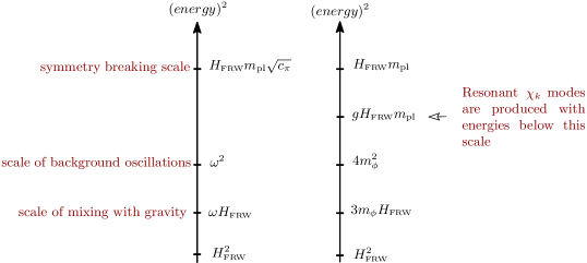
Figure 4: Relevant energy scales for the preheating models considered in Section IV.3. On the left, we have the hierarchy in energy scales associated with the dynamics of the Goldstone boson with a sound speed $c_{\pi}$ following our general discussion of self-resonant models. The right diagram shows the hierarchy of scales for the example of canonical two-field preheating models.

An explicit example: The generic construction above is useful in studying models of inflaton self-resonance. Consider an example where mixing with gravity at the end of inflation leads to resonant effects for $\pi_{c}$. For this purpose, we consider a simple limit of the unitary gauge action in (39) where $m_{2}=0$, $m_{\rm pl}^{2}(3H^{2}+\dot{H})=V(\phi_{{}_{0}})=m_{\phi}^{2}\phi_{{}_{0}}^{2}/2~{}$, and $\dot{H}m_{\rm pl}^{2}=-\dot{\phi}_{{}_{0}}^{2}/2$. These choices correspond to a cosmology dominated by a single scalar field – the inflaton. In the regime where $m_{\phi}\gg H$, the background condensate oscillates around the minimum of its potential $V=m_{\phi}^{2}\phi_{{}_{0}}^{2}/2$, and in this case we can solve for the background evolution Mukhanov:2005sc

$$H(t) = H_{{\mbox{\tiny FRW}}}(t)-\frac{3H_{\mbox{\tiny FRW}}(t)^{2}}{4m_{\phi}}\sin(2m_{\phi}t)+\ldots,$$ (56)

where $H_{\mbox{\tiny FRW}}=2/(3t)$ is the Hubble rate in a matter dominated universe with scale factor $a(t)\propto t^{2/3}$ and dots represent terms suppressed by higher powers of $H_{m}/m_{\phi}$. This solution has exactly the form proposed in (47) with $H_{{\mbox{\tiny osc}}}\equiv-3H_{\mbox{\tiny FRW}}^{2}/4m_{\phi}$, $\omega\equiv 2m_{\phi}$, and we also have $H_{\mbox{\tiny FRW}}\ll m_{\phi}$.

Given the background evolution in (56), we can now consider the dynamics of $\pi_{c}$. To reproduce this class of models we take the $c_{\pi}\to 1$ limit, and solve for the constraints $\delta N_{c}$ and $N^{i}_{c}$. Using our results from Appendix A, along with (50) we have

$$\mathcal{L}_{\pi_{c}}=-\frac{1}{2}(\partial\pi_{c})^{2}-\frac{1}{2}\Big{(}m_{\pi}^{2}(t)+m_{\rm mix}^{2}(t)\Big{)}\pi_{c}^{2},$$ (57)

where the mass mixing induced by $\delta N_{c}$ and $N^{i}_{c}$ is

$$m_{\rm mix}^{2}=6\dot{H}+2\frac{\ddot{H}}{H}-2\frac{\dot{H}^{2}}{H^{2}}.$$ (58)

Using the background evolution given by (56) and (58) the mode equation for the re-scaled field variable $\tilde{\pi}_{c}=a^{3/2}\pi_{c}$ can be written as

$$\ddot{\tilde{\pi}}_{c}+\left[\frac{k^{2}}{a^{2}}+m_{\phi}^{2}\left(1+6\frac{H_{\mbox{\tiny FRW}}}{m_{\phi}}\sin(2m_{\phi}t)\right)\right]\tilde{\pi}_{c}=0,$$ (59)

where we have dropped additional terms further suppressed by $H_{\mbox{\tiny FRW}}^{2}/m_{\phi}^{2}$ and $m_{\pi}^{2}\to V^{\prime\prime}(\phi_{{}_{0}})=m_{\phi}^{2}$ which follows from relating derivatives of the potential to the time derivatives of the Hubble rate given in (56) (See Appendix B).

To establish whether self-resonance results in particle production we can recast (59) in the form of a Mathieu equation by re-defining the time variable $z=m_{\phi}t+\pi/4$ with $A_{k}=1+k^{2}/(a^{2}m_{\phi}^{2})$ and $q=3H_{\mbox{\tiny FRW}}/m_{\phi}$. As the background evolution implies the hierarchy $H_{\mbox{\tiny FRW}}\ll m_{\phi}$, this implies modes in equation (59) will be in the narrow resonance regime, $q\ll 1$. The first instability corresponds to the condition $A_{k}<1+q$ implying modes with momenta

$$\frac{k}{a}<\sqrt{3H_{\mbox{\tiny FRW}}m_{\phi}}$$ (60)

will be amplified Kofman:1997yn . This result matches well with our previous estimate on the momentum scales where mixing with gravitational fluctuations is important in (55) (recalling we have $c_{\pi}=1$ here).

Such resonant effects due to mixing with gravity have been considered previously in the literature Easther:2010mr ; Jedamzik:2010hq , where those authors studied the growth of the density perturbations and the onset of non-linear effects arising during oscillations of the background. Here, we can use the EFT to reproduce their results

$$\delta_{k}\equiv\frac{\delta\rho_{k}}{\bar{\rho}(t)}=\frac{\delta\rho_{k}}{3H^{2}m_{\rm pl}^{2}}\propto\left(\frac{k}{aH_{\mbox{\tiny FRW}}}\right)^{2},~{}~{}{\rm for}~{}~{}~{}\frac{k}{a}<\sqrt{3H_{\mbox{\tiny FRW}}m_{\phi}},$$ (61)

where $\delta\rho_{k}$ is defined as

$$\delta\rho_{k}=(-2\dot{H})^{1/2}m_{\rm pl}\left[\dot{\pi}_{c}-\frac{1}{2}\left(3+\frac{\ddot{H}}{\dot{H}}-2\frac{\dot{H}}{H}\right)\pi_{c}\right].$$ (62)

We now consider how the EFT captures models where the reheat sector results from the inflaton resonance given by the time-dependent functions in (45) and (46). If any of these couplings are stronger than gravitational strength the resonance in the reheat sector will typically dominate over the gravitationally induced effects discussed above.

IV.3.2 Reheating in a Two-Field Model

In this section, we explicitly demonstrate how the EFT approach reproduces models of two-field reheating, taking as a concrete example the specific class of models given by (1). In the early stages of preheating the inflaton will dominate the energy density. We take the reheat field to be initially in its vacuum with $\chi_{{}_{0}}=0$, and we consider production of $\chi$ quanta in the presence of the oscillating inflaton condensate $\phi_{{}_{0}}(t)$. In the unitary gauge with $\phi=\phi_{{}_{0}}(t)$ and $\chi_{{}_{0}}=0$, we have the following matter Lagrangian

$$S_{m}=\int d^{4}x\sqrt{-g}\left[-\frac{1}{2}\dot{\phi}_{{}_{0}}^{2}g^{00}-V(\phi_{{}_{0}})-\frac{1}{2}g^{\mu\nu}\partial_{\mu}\chi\partial_{\nu}\chi-\frac{1}{2}(U^{\prime\prime}(\chi_{{}_{0}})+g^{2}\phi_{{}_{0}}^{2})\chi^{2}\right].$$ (63)

Using the background equations of motion we can cancel the tadpole terms, $m_{\rm pl}^{2}(3H^{2}+\dot{H})=V(\phi_{{}_{0}})=m_{\phi}^{2}\phi_{{}_{0}}^{2}/2~{}$, $\dot{H}m_{\rm pl}^{2}=-\dot{\phi}_{{}_{0}}^{2}/2$, and the unitary gauge matter Lagrangian is then given by

$$\mathcal{L}_{m}=m_{\rm pl}^{2}\dot{H}g^{00}-m_{\rm pl}^{2}(3H^{2}+\dot{H})-\frac{1}{2}g^{\mu\nu}\partial_{\mu}\chi\partial_{\nu}\chi-\frac{1}{2}\left(m_{\chi}^{2}+2\frac{g^{2}m_{\rm pl}^{2}}{m_{\phi}^{2}}(3H^{2}+\dot{H})\right)\chi^{2},$$ (64)

where we defined $U^{\prime\prime}(\chi_{{}_{0}})\equiv m_{\chi}^{2}$. Comparing with the unitary gauge action (39) – (41), the matter Lagrangian (64) corresponds to the following choice for non-universal parameters in the EFT framework,

$$\alpha_{1}=1,~{}~{}~{}~{}\alpha_{3}=m_{\chi}^{2}+2\frac{g^{2}m_{\rm pl}^{2}}{m_{\phi}^{2}}(3H^{2}+\dot{H}),~{}~{}~{}\{m_{2},\alpha_{2},\alpha_{4},\beta_{1},\beta_{2}\}=0.$$ (65)

We emphasize that in this model the linear mixing between the $\chi$ sector and gravitational sector (which includes the Goldstone in the unitary gauge) vanishes automatically since $\beta_{1},\beta_{2}=0$ in (41). As before, we can introduce the Goldstone sector in (64) following the transformation rules in (IV.1.2). However, in the presence of strong resonance in the $\chi$ sector, i.e. if $\dot{\alpha_{3}}/\alpha_{3}^{2}>\mathcal{O}(1)$ during any time in the linear stage of preheating, Goldstone fluctuations will be negligible compared to the $\chi$’s that are amplified through the strong resonance. In general, the validity of this argument relies on the strength of the coupling between the background and the $\chi$ sector through the mass term. For example, in the model we are considering here, introducing $\pi$ via $t\to t+\pi$ (See also (IV.1.2)) will lead to the Goldstone sector we have discussed in the previous section, where mixing with gravity leads to weak resonance $q\approx H_{\mbox{\tiny FRW}}/m_{\phi}\ll 1$ (c.f. (59) and the discussion that follows). On the other hand, the strength of the resonance in the $\chi$ sector depends on the ratio $gm_{\rm pl}/m_{\phi}$ which can be quite large unless $g\ll 1$. Too see this in detail, it is enough to compare the scales in our EFT. The strength of the resonance in $\chi$ can be read from (65) and compared to the strength $\approx m_{\phi}H_{\mbox{\tiny FRW}}$ of the resonance in the Goldstone sector in equation (59). The following condition is sufficient to neglect the Goldstone dynamics

$$g^{2}\left(\frac{m_{\rm pl}}{m_{\phi}}\right)\left(\frac{\Lambda_{\rm sb}}{m_{\phi}}\right)^{2}>1.$$ (66)

It is clear from this expression that unless the coupling constant is tiny $g\ll 1$ we can neglect the mild amplification of Goldstone due to mixing with gravity.

Another simplification we can make in this case is to consider the decoupling limit in the EFT where $|\dot{H}|\approx H_{\mbox{\tiny FRW}}^{2}\to 0$ and $m_{\rm pl}^{2}\to\infty$, while keeping the combinations $\dot{H}m_{\rm pl}^{2}$ and $H^{2}m_{\rm pl}^{2}$ as constant. In this limit, it is clear that $\pi$ fluctuations will stay in their vacuum as the terms leading to narrow resonance vanishes ($H_{\mbox{\tiny FRW}}\to 0$). We also note that the decoupling limit corresponds to taking the rigid space-time limit, $a\to 1$ that is commonly discussed in the preheating literature Kofman:1997yn ; Amin:2014eta .

To study particle production, we can focus on the decoupling limit of the Lagrangian (64), and consider the mode equation for $\chi$ as,

$$\ddot{\chi}_{k}+\omega_{\chi}^{2}(t)\chi_{k}=0$$ (67)

where the time dependent frequency is given by

$$\omega_{\chi}^{2}=k^{2}+m_{\chi}^{2}+\frac{g^{2}m_{\rm pl}^{2}}{m_{\phi}^{2}}(3H^{2}+\dot{H}).$$ (68)

In the decoupling limit, the time dependent mass induced by the background evolution stays intact, which is crucial for particle production. As we have mentioned before, particle production corresponds to the breakdown of the adiabaticity in the frequency, i.e. $|\dot{\omega}_{\chi}/\omega_{\chi}^{2}|>\mathcal{O}(1)$. Using (56) and the relations with the potential and Hubble rate in Appendix B, this condition translates into

$$K^{2}\lesssim g~{}H_{\mbox{\tiny FRW}}m_{\rm pl}\approx g\Lambda_{\rm sb}^{2},$$ (69)

where $K=\sqrt{k^{2}+m_{\chi}^{2}}$ is the rescaled momenta. In the example we are considering, we see that this condition justifies the use of the EFT formalism as the resonant modes have a momenta much smaller than the symmetry breaking scale for small enough coupling, i.e. $H_{\mbox{\tiny FRW}}m_{\rm pl}\equiv\Lambda_{\rm sb}^{2}\gg g\Lambda_{\rm sb}^{2}$ for $g\ll 1$. The structure of the instability band along with the exponentially growing solutions in the $\chi$ sector have been studied many times in the literature Amin:2014eta . Here, our main purpose is to show the connection of the EFT approach to well established two-field reheating models.

Another potential use of EFT formalism is to capture the effects of backreaction. This can be achieved by realizing that once we introduce the Goldstone mode in the unitary gauge Lagrangian (64) the time dependent mass (and for general models other time dependent functions) of $\chi$ becomes $\alpha_{3}(t+\pi)$. As $\alpha_{3}$ is a rapidly varying function of time in the presence of particle production in the $\chi$ sector, this term will induce higher order interactions between $\pi$ and $\chi$ upon expanding the function,

$$\mathcal{L}_{int}=-\frac{1}{2}\left(\dot{\alpha}_{3}\pi+\frac{1}{2}\ddot{\alpha}_{3}\pi^{2}\right)\chi^{2}.$$ (70)

In particular, in the current example the first term in (70) will lead to a tadpole term for $\pi_{c}=(-2\dot{H})^{1/2}m_{\rm pl}\pi$. In the Hartree approximation Kofman:1997yn this gives

$$\mathcal{L}_{int}\supset-\frac{1}{2}\frac{\dot{\alpha}_{3}}{(-2\dot{H}m_{\rm pl}^{2})^{1/2}}\langle\chi^{2}\rangle\pi_{c},$$ (71)

where

$$\langle\chi^{2}(t)\rangle=\frac{1}{2\pi^{2}}\int_{0}^{\infty}dk~{}k^{2}~{}|\chi_{k}(t)|^{2}.$$ (72)

The existence of such a tadpole term can be considered as an indication of backreaction effects. For example, as we produce $\chi$ particles the coefficient in front of $\pi_{c}$ will grow and may eventually disturb the background evolution. In particular they can increase the frequency of the background oscillations of the condensate Kofman:1997yn ,

$$m_{\phi}^{2}\to m_{\phi}^{2}+\frac{\dot{\alpha}_{3}}{(-2\dot{H}m_{\rm pl}^{2})^{1/2}}\langle\chi^{2}\rangle$$ (73)

In order to understand the onset of the backreaction effects in the presence of particle production, we can compare the second term in (73) with $m_{\phi}^{2}$. We refer to this time where the backreaction becomes important as $t_{b}$ and the condition reads

$$m_{\phi}^{2}=\frac{\dot{\alpha}_{3}(t_{b})}{(-2\dot{H}(t_{b})m_{\rm pl}^{2})^{1/2}}\langle\chi^{2}(t_{b})\rangle$$ (74)

Knowing the solutions for $\chi_{k}$, the background evolution (56) and the couplings $\alpha_{3}$ one can calculate $t_{b}$.

We emphasize that our discussion in this section is not limited to the example given by (65). Using the EFT formalism, we can in principle capture models that belong to the same “universality class”, i.e. direct coupling models with interactions including $\mathcal{L}_{m}\propto\mu\phi\chi^{2}$ and non-renormalizable couplings $\mathcal{L}_{m}\propto\phi^{n}\chi^{2}/M^{n-2}$ where $n>2$ and $M,\mu$ are energy scales Dufaux:2006ee .

IV.4 A New Class of Reheating Models

In the previous section, we showed how the EFT captures resonance effects in two-field reheating models. We now reconsider particle production in the presence of a reduced sound speed for the reheat field, $c_{\chi}\neq 1$. Familiar from the EFT of Inflation and Dark Energy, there is no symmetry protecting $c_{\chi}=1$ in the EFT of reheating. This gives rise to a new class of models for preheating where the produced particles can have $c_{\chi}\ll 1$.

We follow our previous discussion in Section IV.2 and consider the time-dependent functions associated with the reheat sector $\{\alpha_{i},\beta_{i}\}$. The terms proportional to $\beta_{1}$ and $\beta_{2}$ in (46) lead to mixing of $\chi$ with both gravity and the Goldstone sector. We will ignore these terms here, leaving a discussion of them to Appendix A. In the absence of these mixing terms we focus on the action (45). Defining the canonical field $\chi_{c}=\alpha_{\chi}(t)\chi$ where $\alpha_{\chi}^{2}(t)=\alpha_{1}(t)+\alpha_{2}(t)$, we have the following second order Lagrangian for the canonical reheat field

$$\mathcal{L}_{\chi_{c}}=\frac{1}{2}\left[\dot{\chi}_{c}^{2}-c_{\chi}^{2}(t)\frac{(\partial_{i}\chi_{c})^{2}}{a^{2}}\right]-\frac{1}{2}m_{\chi}^{2}(t)\chi_{c}^{2},$$ (75)

where we have defined the sound speed $c_{\chi}^{2}=\alpha_{1}/(\alpha_{1}+\alpha_{2})$ and the time-dependent mass term is

$$m_{\chi}^{2}(t)=\frac{\alpha_{3}(t)}{\alpha_{\chi}^{2}(t)}-{\left(\frac{\dot{\alpha_{\chi}}}{\alpha_{\chi}}\right)^{2}}+3H{\left(\frac{\dot{\alpha_{\chi}}}{\alpha_{\chi}}\right)}+\partial_{t}{\left(\frac{\dot{\alpha_{\chi}}}{\alpha_{\chi}}\right)}.$$ (76)

Similar to the Goldstone case in Section IV.3.1, we have a time-dependent mass $m_{\chi}(t)$ induced by the time dependence of the sound speed $c_{\chi}$ and $\alpha_{1}$ . We will concentrate on strong resonant effects due to non-adiabaticity in the time-dependent coefficient $\alpha_{3}$ and assume that the time variation of $\alpha_{\chi}$ is slow compared to $\alpha_{3}$, so that the sound speed is nearly constant (where $\alpha_{1},\alpha_{2}\approx constant$). We can then neglect the last three terms in (76) and the mode equation for the re-scaled field variable $\tilde{\chi}_{c}=a^{3/2}\chi_{c}$ in Fourier space is

$$\ddot{\tilde{\chi}}^{k}_{c}+\left[c_{\chi}^{2}\frac{k^{2}}{a^{2}}+\alpha_{3}+\Delta\right]\tilde{\chi}^{k}_{c}=0,$$ (77)

where $\Delta=-3(3H^{2}+2\dot{H})/4\approx\mathcal{O}(H^{2})$ are gravitational terms resulting from the rescaling $\chi_{c}\to\tilde{\chi}_{c}$ and we have absorbed the constants $\alpha_{1},\alpha_{2}$ into the definition of $\alpha_{3}$. Following our discussion in Section IV.2, it is convenient to parameterize $\alpha_{3}$ as $\alpha_{3}=M^{2}(t)F(\omega t)$, where $M(t)$ is always adiabatic so that $\dot{M}/M^{2}\ll 1$ and $F$ is a periodic function which must violate adiabaticity so that preheating occurs. That is, at some point adequate particle production requires the so-far arbitrary function to satisfy $\dot{F}/F^{2}>1$. In many models the periodicity of the function will be set by the background evolution in (47). We focus on the strong resonance regime where $M\gg H$ and $M/\omega\gg 1$ and hence drop $\mathcal{O}(H^{2})$ terms in the frequency $\omega_{\chi}^{2}$,

$$\omega_{\chi}^{2}=c_{\chi}^{2}\frac{k^{2}}{a^{2}}+M^{2}F(\omega t).$$ (78)

The non-adiabaticity in $\alpha_{3}$ will lead to non-adiabaticity in the frequency $\omega_{\chi}^{2}$, i.e. $\dot{\omega}_{\chi}/\omega_{\chi}^{2}>\mathcal{O}(1)$. We take this to occur as times $t_{j}$ when $\omega_{\chi}^{2}$ is at its minimum. This suggests that we can expand the frequency around the times $t_{j}$ as

$$\omega^{2}_{\chi}\simeq c_{\chi}^{2}\frac{k^{2}}{a^{2}}+\frac{1}{2}M^{2}\omega^{2}(t-t_{j})^{2}+\dots$$ (79)

where we have used $\ddot{F}\approx\omega^{2}F$ and dots represent higher order terms in the $t-t_{j}$ expansion. This allows us to re-write the mode equation in a simpler form

$$\ddot{\tilde{\chi}}^{k}_{c}+\left[c_{\chi}^{2}\frac{k^{2}}{a^{2}}+\frac{M^{2}\omega^{2}}{2}(t-t_{j})^{2}\right]\tilde{\chi}^{k}_{c}=0$$ (80)

and the typical momenta when adiabaticity is violated $\dot{\omega}_{\chi}>\omega^{2}_{\chi}$ corresponds to

$$k_{\ast}^{2}\equiv\frac{M\omega}{c_{\chi}^{2}}\gtrsim\frac{k^{2}}{a^{2}},$$ (81)

We see that for $c_{\chi}<1$, the physical wave numbers inside the resonant regime are further enhanced (the resonance band is broadened) compared to the standard cases that have been studied in the literature. It is customary to map the mode equation (80) to a scattering problem described by a Schrödinger equation with a negative parabolic potential by defining a new time variable $\tau\equiv c_{\chi}k_{*}(t-t_{j})$ and a dimensionless physical momentum $\kappa\equiv k/(ak_{*})$,

$$\frac{d^{2}\tilde{\chi}^{k}_{c}}{d\tau^{2}}+\left(\kappa^{2}+\tau^{2}\right)\tilde{\chi}^{k}_{c}=0.$$ (82)

The solution to the scattering problem and the resulting number density of particles between scattering events has appeared in the literature many times Kofman:1997yn ; Bassett:2005xm (See also Amin:2015ftc ). In real space, the growth of the number density of particles can be described by the following expression Kofman:1997yn ,

$$n_{\chi}(t)=\frac{1}{2\pi a^{3}}\int d^{3}k~{}n^{k}_{\chi}(t)\sim\frac{k_{*}^{3}}{\sqrt{\pi\mu m_{\phi}t}}e^{2\mu m_{\phi}t},$$ (83)

where (for simplicity) we have assumed that the background is given by the quadratic potential we considered before, i.e. $\omega\sim m_{\phi}$. Here $\mu$ is the maximum value of the Floquet index at $k_{\max}\approx k_{*}/2$ Kofman:1997yn . It is clear from this expression that there will be an enhancement in the number of produced particles due to the small sound speed in the $\chi$ sector, $k_{*}\propto c_{\chi}^{-1}$. This also agrees with our intuition as equation (81) tells us that resonant bands are wider for $c_{\chi}<1$ and thus the contribution to the integral in (83) over resonant modes will be enhanced by factors of $c_{\chi}^{-1}$. In the next section we will consider observational consequences of the EFT of reheating, focusing on this new class of models with non-standard sound speed. We also discuss additional challenges and future directions for the approach.

V Challenges and Outlook

In this paper we have presented an EFT approach to reheating that overcomes the challenges of the background evolution discussed in Section III and is adequate to capture all existing reheating models in the literature. Guided by symmetries, our approach is also useful for finding new models of reheating, e.g. we found a new class of models where the reheating sector has $c_{\chi}\neq 1$. However, there are many challenges remaining for our EFT approach.

One of the more serious concerns is the lack of a direct connection to observations. This problem is not specific to our approach, with the lack of direct observational constraints on reheating being an important reason that far less is known about this epoch than inflation. In our EFT framework, symmetries help to alleviate more of the theoretical uncertainties associated with reheating than a toy model approach. For example, the need to non-linearly realize time translations demonstrated that many of the unknown coefficients are related, and the need to violate non-adiabaticity (required for particle production) also placed some level of theoretical constraint on the reheating sector. Nevertheless, we saw in Section IV there are a large number of free functions that must be further restricted by observations. Unlike the situation for inflation, where non-Gaussianity and features in the primordial power spectrum are a rich source of observational constraints, direct observational constraints on reheating are lacking. One possibility to remedy this is gravitation wave (GW) signatures.

Once particles are produced during reheating they can scatter off each other creating a background of GWs Easther:2006gt ; Easther:2006vd . The scattering leads to a transverse-traceless source for the gravitons

$$\ddot{h}_{ij}+3H\dot{h}_{ij}-\frac{1}{a^{2}}\partial^{2}h_{ij}=\frac{2}{m_{\rm pl}^{2}}T^{TT}_{ij}$$ (84)

Following the methods of Dufaux:2007pt we can then estimate the critical density of gravitational waves today

$$\Omega_{\rm gw}=\frac{S_{k}(t_{f})}{a_{J}^{4}~{}\rho_{J}}~{}\left(\frac{a_{J}}{a_{\rm rh}}\right)^{1-3w}\left(\frac{g_{\rm rh}}{g_{0}}\right)^{-1/3}\Omega_{r,0},$$ (85)

where subscript “$0$” denotes a quantity evaluated today, ‘$J$ ’ represents the time when the universe becomes radiation dominated and ‘${\rm rh}$’ denotes the beginning of reheating. Here, $\omega$ is the average equation of state of the universe between the time interval $t_{J}<t<t_{\rm rh}$ and $g_{i}$ is the effective relativistic degrees of freedom. Finally, the source term $S_{k}$ encodes the predictions for different classes of models in the EFT.

For example, let us consider the new class of models discussed in Section IV.4. In that case the source term $S_{k}$ is given by

$$S_{k}(t_{f}) = \frac{c_{\chi}^{4}~{}k^{3}}{4\pi^{2}m_{\rm pl}^{2}}\int dp\int_{-1}^{1}d(\cos\theta)~{}p^{6}\sin^{4}\theta$$

$$\times \Bigg{[}\left|\int_{t_{i}}^{t_{f}}dt\cos\left(kt\right)\chi_{c}(p,t)\chi_{c}(|\vec{k}-\vec{p}|,t)\right|^{2}+\left|\int_{t_{i}}^{t_{f}}dt\sin\left(kt\right)\chi_{c}(p,t)\chi_{c}(|\vec{k}-\vec{p}|,t)\right|^{2}\Bigg{]}$$

where we focus on two-body scattering, $\theta$ is the scattering angle, and we assume that scattering happens at a fast enough rate that we can neglect the Hubble expansion. To get an order of magnitude estimate we can focus on the low momenta. In this case, the contribution of the mode functions to time integrals will be maximal for $p_{*}=\sqrt{M\omega}/c_{\chi}$ and defining a dimensionless momentum $P=p/p_{*}$ we have

$$S_{k}^{j+1}\sim\frac{1}{c_{\chi}^{3}}\frac{(M\omega)^{3/2}k^{3}}{m_{\rm pl}^{2}}\int_{-1}^{1}d(\cos\theta)\sin^{4}\theta\int~{}dPP^{6}\times[Time~{}integrals],$$ (87)

where we recall that $\alpha_{3}$ is parameterized by $M$ and $\omega$ as in (80), and so the EFT parameters are determining the strength of the GW signal. Moreover, the gravitational waves will be amplified by a factor of $c_{\chi}^{-3}$. This scaling may be counter-intuitive to the reader. The prefactor in (V) results from the two-to-two scattering of the particles as their momenta is now $p\rightarrow c_{\chi}p$. However, the lower sound speed implies it costs less energy to produce the particles leading to an enhancement of the particle production rate, and more particles scattering leads to more gravity waves. Thus, the GW signal is enhanced compared to the $c_{\chi}=1$ case. Assuming this signal survives the later stages of reheating the detectability will depend on the peak frequency Easther:2006gt ; Easther:2006vd ; Giblin:2014gra

$$f=\frac{\sqrt{M\omega}}{a_{j}\rho_{j}^{1/4}c_{\chi}}\;4\times 10^{10}\;\mbox{Hz},$$ (88)

which again depends explicitly on the EFT parameters and the sound speed. We see that by reducing the sound speed we can increase the frequency in the new class of reheating models.

GWs provide one way to constrain the EFT parameters. However, we leave a more complete analysis, which requires following the signal through all the stages of reheating, to future work. Primordial Black Hole constraints and the matching of inflationary perturbations to late time observables lead to additional ways in which the EFT parameters may be restricted. In regards to the latter, we have stressed that direct observables correspond to perturbations, however the subtle ways in which we match inflationary predictions to CMB and LSS observations does depend implicitly on the background dynamics, particularly through the equation of state. Recently, it has been shown that the physics of reheating (including non-linearities and back-reaction) can have subtle and interesting effects on the equation of state and the dynamics of thermalization Lozanov:2016hid . We hope to return to these issues and interesting possibilities in future work.

In addition to the challenge to connect with observations, a number of theoretical issues remain to be addressed. In particular, in this paper we have primarily focused on connecting the EFT to scalar field driven models of reheating. However, the spectator field $\chi$ can be thought of as an additional clock field, which can also represent reheat fields beyond spin zero. Extending our framework to other spins is an important consideration. We have also primarily focused on the first stage of reheating in the EFT. However, one of the most useful applications of our approach could be to gain a better understanding of the rescattering and back-reaction effects that happen following the first stage. These are stages that usually require lattice simulations, and the Goldstone approach could be a fruitful way to get a better analytical understanding. There is also the issue of when the produced particles become significant enough that they contribute to the energy density. At this point the Goldstone boson (related to the matter sector responsible for time-translations being broken) can change its nature from inflatons to the reheat field. How this transition proceeds is important for establishing the connection between the Goldstone and the background fields. This is similar to the situation in studies of dissipation in the EFT of Inflation (see e.g. LopezNacir:2011kk ), and we expect many of the techniques there could prove useful for the case of reheating as well.

Appendix A: ADM Formalism and Mixing with Gravity

To account for gravitational fluctuations and discuss the regime where they are irrelevant to the dynamics of the Goldstone we decompose the metric in the ADM form. In the spatially flat gauge we have

$$ds^{2}=-(N^{2}-N_{i}N^{i})dt^{2}+2N_{i}dx^{i}dt+\hat{g}_{ij}\,dx^{i}dx^{j},$$ (89)

where $\hat{g}_{ij}=a^{2}(\delta_{ij}+h_{ij})$ is the spatial metric and our gauge choice implies $h_{ii}=\partial_{i}h_{ij}=0$. Inverse metric elements can be written as

$$g^{00}=-\frac{1}{N^{2}}\,,\quad g^{0i}=g^{i0}=\frac{N^{i}}{N^{2}}\,,\quad g^{ij}=h^{ij}-\frac{N^{i}N^{j}}{N^{2}}\,.$$ (90)

To find the relevant terms in the gravitational sector, we expand the Einstein Hilbert term as

$$S_{\rm g}\supset\frac{m_{\rm pl}^{2}}{2}\int\!d^{4}x\>\sqrt{-g}\,R=\frac{m_{\rm pl}^{2}}{2}\int\!d^{4}x\>\sqrt{\hat{g}}\,\big{[}NR^{(3)}+\frac{1}{N}(E^{ij}E_{ij}-E^{i}{}_{i}{}^{2})\big{]},$$ (91)

where $R^{(3)}$ is the three curvature associated with spatial metric $\hat{g}_{ij}$ and $E_{ij}$ is related to the extrinsic curvature of constant time slices through

$$E_{ij}\equiv NK_{ij}=\frac{1}{2}[{\partial_{t}{\hat{g}}}_{ij}-\hat{\nabla}_{i}N_{j}-\hat{\nabla}_{j}N_{i}]\;,$$ (92)

where $\hat{\nabla}_{i}$ is the covariant derivative with respect to spatial metric $\hat{g}_{ij}$. Using the above expressions, we can expand (IV.1.2) up to second order in scalar fluctuations

$$S_{\rm g}=\int d^{4}x\,a^{3}\Bigg{[} - \frac{m_{\rm pl}^{2}\dot{H}}{c_{\pi}^{2}}\Big{(}\dot{\pi}^{2}-c_{\pi}^{2}\frac{(\partial_{i}\pi)^{2}}{a^{2}}\Big{)}-3m_{\rm pl}^{2}\dot{H}^{2}\pi^{2}+m_{\rm pl}^{2}(2c_{\pi}^{-2}\dot{H}\dot{\pi}-6H\dot{H}\pi)\delta N+2m_{\rm pl}^{2}\dot{H}N^{i}\partial_{i}\pi$$ (93)

$$- m_{\rm pl}^{2}(3H^{2}+c_{\pi}^{-2}\dot{H})\delta N^{2}-2m_{\rm pl}^{2}H\delta N\partial_{i}N^{i}\Bigg{]}\,$$

where the speed of sound is defined as $c_{\pi}^{2}=m_{\rm pl}^{2}\dot{H}/(m_{\rm pl}^{2}\dot{H}-m_{2}^{4})$. Defining the canonical fields, $\pi_{c}=\sqrt{-2\dot{H}m_{\rm pl}^{2}}~{}c_{\pi}^{-1}\pi,\delta N_{c}=m_{\rm pl}\delta N,N^{i}_{c}=m_{\rm pl}N^{i}$, one can re-write the Lagrangian as in (50).

Focusing on the Goldstone sector for now, we can solve for the Lagrange multipliers $\delta N$ and $N^{i}$ in terms of $\pi$. To linear order in $\pi$ we have,

$$\delta N=-\frac{\dot{H}}{H}\pi,~{}~{}~{}~{}~{}~{}~{}\partial_{i}N^{i}=c_{\pi}^{-2}\frac{\dot{H}}{H^{2}}\partial_{t}\left(H\pi\right).$$ (94)

Using the canonical field definitions above we may write

$$\delta N_{c}=\frac{(-2\dot{H})^{1/2}}{2H}\pi_{c},~{}~{}~{}~{}~{}~{}~{}\partial_{i}N^{i}_{c}=c_{\pi}^{-2}\frac{\dot{H}}{H^{2}}\partial_{t}\left(\frac{c_{\pi}H\pi_{c}}{(-2\dot{H})^{1/2}}\right).$$ (95)

Using these solutions for the gravitational fluctuations $\delta N_{c}$ $N^{i}_{c}$ in (50) (while taking the $c_{\pi}\to 1$ limit) we recover the result of (57).

In the presence of a reheat sector $\chi$, we need to take into account the mixing between $\chi$ and gravitational fluctuations, as well as $\pi-\chi$ mixings. Considering the mixings at second order we need to take into account the action in (46). Expanding up to second order in $\delta N$, $N^{i}$, $\pi$ and $\chi$, we have

$$S_{\rm mix}^{(2)}=\int d^{4}x\,a^{3}\Big{[}2\beta_{1}\left(\delta N-\dot{\pi}\right)\chi-2\beta_{2}\left(\delta N-\dot{\pi}\right)\dot{\chi}\Big{]}\,.$$ (96)

We note that the action (45) does not lead to any second order mixing therefore it is enough to consider the mixing action above. Combining (93) and (96) in the presence of mixing we have the following solutions for the constraints,

$$\delta N=-\frac{\dot{H}}{H}\pi,~{}~{}~{}~{}~{}\partial_{i}N^{i}=c_{\pi}^{-2}\frac{\dot{H}}{H^{2}}\partial_{t}\left(H\pi\right)+\frac{\beta_{1}}{m_{\rm pl}^{2}H}\chi-\frac{\beta_{2}}{m_{\rm pl}^{2}H}\dot{\chi}.$$ (97)

We see that inclusion of reheat sector does not change the solution for $\delta N$, but we have additional contributions to $N^{i}$ proportional to the time-dependent parameters $\beta_{1},\beta_{2}$ . To illustrate the decoupling of $\chi$, we consider a simple $\pi_{c}$ sector with $c_{\pi}=1$ and note that time derivatives of canonically normalized fields $\chi_{c}$ and $\pi_{c}$ have the approximate scalings in the WKB approximation,

$$\dot{\pi}_{c}\approx\omega_{\pi}\pi_{c}\sim\omega\pi_{c},~{}~{}~{}~{}\dot{\chi}_{c}\approx\omega_{\chi}\chi_{c}\sim\sqrt{\alpha_{3}}\chi_{c}\sim M\chi_{c},$$ (98)

where we take $|\alpha_{3}|=M^{2}$ following our discussion in the main text and focused on the non-relativistic modes for both fields. Following our discussion in section IV.2, we assume that the strength of the couplings $\beta_{1}$ and $\beta_{2}$ is as strong as the time-dependent parameter $\alpha_{3}$ responsible for the resonance. By dimensional analysis, we therefore take $|\beta_{1}|\sim M^{3}$ and $|\beta_{2}|\sim M^{2}$. Canonically normalizing the fields as before we find from (96) that for resonant modes mixing between $\chi_{c}$ and gravitational fluctuations can be neglected in the following range of momenta

$$\left(\frac{M}{\Lambda_{\rm sb}}\right)\sqrt{MH}<\frac{c_{\chi}k}{a}<\sqrt{M\omega}.$$ (99)

Similarly we have the following range where we can neglect direct mixing between $\pi_{c}$ and $\chi_{c}$,

$$\left(\frac{M}{\Lambda_{\rm sb}}\right)\sqrt{M\omega}<\frac{c_{\chi}k}{a}<\sqrt{M\omega}.$$ (100)

Consistency of the EFT picture requires $M/\Lambda_{\rm sb}\ll 1$ and we see that within this regime we can neglect both types of mixing for a wide range of momenta. In particular, with some mild assumptions, we showed that in the presence of strong resonance, we can neglect the mixings between $\pi_{c}$ and $\chi_{c}$. This finding is similar in spirit to the discussion presented in the recent works Green:2014xqa ; Amin:2015ftc where those authors pointed out that it is technically natural to assume a flat field space metric in the presence of strong disorder/resonance.

We conclude this appendix by giving the second order action for tensor perturbations and their interaction with $\pi_{c}$ and $\chi_{c}$ that we used in the main text. Using the gravitational part of the action in (91) with (92) and noting the Ricci curvature $R^{(3)}$ on spatial hyper-surfaces,

$$R^{(3)} = \hat{g}^{ik}\partial_{l}\Gamma^{l}_{ik}-\hat{g}^{ik}\partial_{k}\Gamma^{l}_{il}+\hat{g}^{ik}\Gamma^{l}_{ik}\Gamma^{m}_{lm}-\hat{g}^{ik}\Gamma^{m}_{il}\Gamma^{l}_{km},$$ (101)

$$\Gamma^{k}_{ij} = \frac{1}{2}\hat{g}^{kl}\left(\partial_{i}\hat{g}_{jl}+\partial_{j}\hat{g}_{il}-\partial_{l}\hat{g}_{ij}\right),$$ (102)

we have the following second order action for the tensor part of the metric fluctuations

$$S_{\rm g}=\frac{m_{\rm pl}^{2}}{8}\int\!d^{4}x\>a^{3}\,\left(\dot{h}_{ij}\dot{h}_{ij}-\frac{\partial_{k}h_{ij}\partial_{k}h_{ij}}{a^{2}}\right).\;$$ (103)

On the other hand, expanding the actions (IV.1.2) and (45) we find the following cubic order interactions between $\pi_{c}$ and $\chi_{c}$

$$S_{hXX}\supset\int d^{4}x~{}a^{3}\left(\frac{c_{\chi}^{2}}{2}h_{ij}\frac{\partial_{i}\chi_{c}\partial_{j}\chi_{c}}{a^{2}}+\frac{c_{\pi}^{2}}{2}h_{ij}\frac{\partial_{i}\pi_{c}\partial_{j}\pi_{c}}{a^{2}}\right).$$ (104)

Appendix B: Relating Unitary Gauge to the Scalar Potential

In cosmologies dominated by a scalar field, we can map the time-dependent background quantities in our Unitary gauge Lagrangian (39) to the explicit scalar field models with a given potential $V(\phi_{{}_{0}})$. A simple example we provided in the main text was

$$V(\phi_{{}_{0}})=m_{\rm pl}^{2}(3H^{2}(t)+\dot{H}(t)),~{}~{}~{}~{}-2\dot{H}m_{\rm pl}^{2}=\dot{\phi}_{{}_{0}}^{2}$$ (105)

Using ${\rm d}\phi_{{}_{0}}=\dot{\phi}_{{}_{0}}dt$ and time derivatives of expressions in (105), we can relate the derivatives of the potential with respect to $\phi$ to the time derivatives of the Hubble rate $H(t)$. Here, we list some of these expressions,

$$V^{\prime}(\phi_{{}_{0}}) = \frac{m_{\rm pl}}{(-2\dot{H})^{1/2}}\left(6H\dot{H}+\ddot{H}\right),$$ (106)

$$V^{\prime\prime}(\phi_{{}_{0}}) = -3\dot{H}-\frac{1}{4}\left(\frac{\ddot{H}}{\dot{H}}\right)^{2}-\frac{3H}{2}\left(\frac{\ddot{H}}{\dot{H}}\right)-\frac{1}{2}\partial_{t}\left(\frac{\ddot{H}}{\dot{H}}\right),$$ (107)

$$V^{\prime\prime\prime}(\phi_{{}_{0}}) = \frac{1}{(-2\dot{H}m_{\rm pl}^{2})^{1/2}}\left[-\frac{H^{(4)}}{2\dot{H}}-\frac{9\ddot{H}}{2}+\frac{\ddot{H}^{3}}{2\dot{H}^{3}}-\frac{3H}{2}\partial_{t}\left(\frac{\ddot{H}}{\dot{H}}\right)+\frac{1}{2}\partial_{t}\left(\frac{\ddot{H}^{2}}{\dot{H}^{2}}\right)\right]$$ (108)

- (1) O. Ozsoy, G. Sengor, K. Sinha and S. Watson, “A Model Independent Approach to (p)Reheating,” arXiv:1507.06651 [hep-th].
- (2) L. F. Abbott, E. Farhi and M. B. Wise, “Particle Production in the New Inflationary Cosmology,” Phys. Lett. 117B, 29 (1982). doi:10.1016/0370-2693(82)90867-X
- (3) A. Albrecht, P. J. Steinhardt, M. S. Turner and F. Wilczek, “Reheating an Inflationary Universe,” Phys. Rev. Lett. 48, 1437 (1982). doi:10.1103/PhysRevLett.48.1437
- (4) A. D. Dolgov and A. D. Linde, “Baryon Asymmetry in Inflationary Universe,” Phys. Lett. 116B, 329 (1982). doi:10.1016/0370-2693(82)90292-1
- (5) A. D. Dolgov and D. P. Kirilova, “On Particle Creation By A Time Dependent Scalar Field,” Sov. J. Nucl. Phys. 51, 172 (1990) [Yad. Fiz. 51, 273 (1990)].
- (6) J. H. Traschen and R. H. Brandenberger, “Particle Production During Out-of-equilibrium Phase Transitions,” Phys. Rev. D 42, 2491 (1990). doi:10.1103/PhysRevD.42.2491
- (7) L. Kofman, A. D. Linde and A. A. Starobinsky, “Towards the theory of reheating after inflation,” Phys. Rev. D 56, 3258 (1997) doi:10.1103/PhysRevD.56.3258 [hep-ph/9704452].
- (8) M. A. Amin, M. P. Hertzberg, D. I. Kaiser and J. Karouby, “Nonperturbative Dynamics Of Reheating After Inflation: A Review,” Int. J. Mod. Phys. D 24, 1530003 (2014) doi:10.1142/S0218271815300037 [arXiv:1410.3808 [hep-ph]].
- (9) R. Allahverdi, R. Brandenberger, F. Y. Cyr-Racine and A. Mazumdar, “Reheating in Inflationary Cosmology: Theory and Applications,” Ann. Rev. Nucl. Part. Sci. 60, 27 (2010) doi:10.1146/annurev.nucl.012809.104511 [arXiv:1001.2600 [hep-th]].
- (10) S. Y. Khlebnikov and I. I. Tkachev, “Classical decay of inflaton,” Phys. Rev. Lett. 77, 219 (1996) doi:10.1103/PhysRevLett.77.219 [hep-ph/9603378].
- (11) R. Easther and E. A. Lim, “Stochastic gravitational wave production after inflation,” JCAP 0604, 010 (2006) doi:10.1088/1475-7516/2006/04/010 [astro-ph/0601617].
- (12) J. Garcia-Bellido and A. D. Linde, “Preheating in hybrid inflation,” Phys. Rev. D 57, 6075 (1998) doi:10.1103/PhysRevD.57.6075 [hep-ph/9711360].
- (13) G. N. Felder, J. Garcia-Bellido, P. B. Greene, L. Kofman, A. D. Linde and I. Tkachev, “Dynamics of symmetry breaking and tachyonic preheating,” Phys. Rev. Lett. 87, 011601 (2001) doi:10.1103/PhysRevLett.87.011601 [hep-ph/0012142].
- (14) R. Easther, J. T. Giblin, Jr. and E. A. Lim, “Gravitational Wave Production At The End Of Inflation,” Phys. Rev. Lett. 99, 221301 (2007) doi:10.1103/PhysRevLett.99.221301 [astro-ph/0612294].
- (15) L. R. Price and X. Siemens, “Stochastic Backgrounds of Gravitational Waves from Cosmological Sources: Techniques and Applications to Preheating,” Phys. Rev. D 78, 063541 (2008) doi:10.1103/PhysRevD.78.063541 [arXiv:0805.3570 [astro-ph]].
- (16) R. Easther, H. Finkel and N. Roth, “PSpectRe: A Pseudo-Spectral Code for (P)reheating,” JCAP 1010, 025 (2010) doi:10.1088/1475-7516/2010/10/025 [arXiv:1005.1921 [astro-ph.CO]].
- (17) M. P. Hertzberg, J. Karouby, W. G. Spitzer, J. C. Becerra and L. Li, “Theory of self-resonance after inflation. I. Adiabatic and isocurvature Goldstone modes,” Phys. Rev. D 90, 123528 (2014) doi:10.1103/PhysRevD.90.123528 [arXiv:1408.1396 [hep-th]].
- (18) M. A. Amin and D. Baumann, “From Wires to Cosmology,” JCAP 1602, no. 02, 045 (2016) doi:10.1088/1475-7516/2016/02/045 [arXiv:1512.02637 [astro-ph.CO]].
- (19) S. Weinberg, “Effective Field Theory for Inflation,” Phys. Rev. D 77, 123541 (2008) doi:10.1103/PhysRevD.77.123541 [arXiv:0804.4291 [hep-th]].
- (20) M. Park, K. M. Zurek and S. Watson, “A Unified Approach to Cosmic Acceleration,” Phys. Rev. D 81, 124008 (2010) doi:10.1103/PhysRevD.81.124008 [arXiv:1003.1722 [hep-th]].
- (21) P. Creminelli, M. A. Luty, A. Nicolis and L. Senatore, “Starting the Universe: Stable Violation of the Null Energy Condition and Non-standard Cosmologies,” JHEP 0612, 080 (2006) doi:10.1088/1126-6708/2006/12/080 [hep-th/0606090].
- (22) C. Cheung, P. Creminelli, A. L. Fitzpatrick, J. Kaplan and L. Senatore, “The Effective Field Theory of Inflation,” JHEP 0803, 014 (2008) doi:10.1088/1126-6708/2008/03/014 [arXiv:0709.0293 [hep-th]].
- (23) L. Senatore and M. Zaldarriaga, “The Effective Field Theory of Multifield Inflation,” JHEP 1204, 024 (2012) doi:10.1007/JHEP04(2012)024 [arXiv:1009.2093 [hep-th]].
- (24) P. Creminelli, G. D’Amico, J. Norena and F. Vernizzi, “The Effective Theory of Quintessence: the w<-1 Side Unveiled,” JCAP 0902, 018 (2009) doi:10.1088/1475-7516/2009/02/018 [arXiv:0811.0827 [astro-ph]].
- (25) J. K. Bloomfield, . . Flanagan, M. Park and S. Watson, “Dark energy or modified gravity? An effective field theory approach,” JCAP 1308, 010 (2013) doi:10.1088/1475-7516/2013/08/010 [arXiv:1211.7054 [astro-ph.CO]].
- (26) G. Gubitosi, F. Piazza and F. Vernizzi, “The Effective Field Theory of Dark Energy,” JCAP 1302, 032 (2013) [JCAP 1302, 032 (2013)] doi:10.1088/1475-7516/2013/02/032 [arXiv:1210.0201 [hep-th]].
- (27) M. Fasiello and Z. Vlah, “Nonlinear fields in generalized cosmologies,” Phys. Rev. D 94, no. 6, 063516 (2016) doi:10.1103/PhysRevD.94.063516 [arXiv:1604.04612 [astro-ph.CO]].
- (28) M. Fasiello and Z. Vlah, arXiv:1611.00542 [astro-ph.CO].
- (29) M. Lewandowski, A. Maleknejad and L. Senatore, “An effective description of dark matter and dark energy in the mildly non-linear regime,” arXiv:1611.07966 [astro-ph.CO].
- (30) D. Baumann, A. Nicolis, L. Senatore and M. Zaldarriaga, “Cosmological Non-Linearities as an Effective Fluid,” JCAP 1207, 051 (2012) doi:10.1088/1475-7516/2012/07/051 [arXiv:1004.2488 [astro-ph.CO]].
- (31) L. Kofman and P. Yi, “Reheating the universe after string theory inflation,” Phys. Rev. D 72, 106001 (2005) doi:10.1103/PhysRevD.72.106001 [hep-th/0507257].
- (32) D. R. Green, “Reheating Closed String Inflation,” Phys. Rev. D 76, 103504 (2007) doi:10.1103/PhysRevD.76.103504 [arXiv:0707.3832 [hep-th]].
- (33) G. N. Felder, L. Kofman and A. D. Linde, “Instant preheating,” Phys. Rev. D 59, 123523 (1999) doi:10.1103/PhysRevD.59.123523 [hep-ph/9812289].
- (34) P. A. R. Ade et al. [Planck Collaboration], “Planck 2015 results. XX. Constraints on inflation,” Astron. Astrophys. 594, A20 (2016) doi:10.1051/0004-6361/201525898 [arXiv:1502.02114 [astro-ph.CO]].
- (35) J. M. Maldacena, “Non-Gaussian features of primordial fluctuations in single field inflationary models,” JHEP 0305, 013 (2003) doi:10.1088/1126-6708/2003/05/013 [astro-ph/0210603].
- (36) V. Assassi, D. Baumann, D. Green and L. McAllister, “Planck-Suppressed Operators,” JCAP 1401, 033 (2014) doi:10.1088/1475-7516/2014/01/033 [arXiv:1304.5226 [hep-th]].
- (37) A. Adams, N. Arkani-Hamed, S. Dubovsky, A. Nicolis and R. Rattazzi, “Causality, analyticity and an IR obstruction to UV completion,” JHEP 0610, 014 (2006) doi:10.1088/1126-6708/2006/10/014 [hep-th/0602178].
- (38) D. A. Easson and A. Vikman, “The Phantom of the New Oscillatory Cosmological Phase,” arXiv:1607.00996 [gr-qc].
- (39) X. Chen and Y. Wang, “Quasi-Single Field Inflation and Non-Gaussianities,” JCAP 1004, 027 (2010) doi:10.1088/1475-7516/2010/04/027 [arXiv:0911.3380 [hep-th]].
- (40) S. Cremonini, Z. Lalak and K. Turzynski, “Strongly Coupled Perturbations in Two-Field Inflationary Models,” JCAP 1103, 016 (2011) doi:10.1088/1475-7516/2011/03/016 [arXiv:1010.3021 [hep-th]].
- (41) A. Achucarro, J. O. Gong, S. Hardeman, G. A. Palma and S. P. Patil, “Features of heavy physics in the CMB power spectrum,” JCAP 1101, 030 (2011) doi:10.1088/1475-7516/2011/01/030 [arXiv:1010.3693 [hep-ph]].
- (42) A. J. Tolley and M. Wyman, “The Gelaton Scenario: Equilateral non-Gaussianity from multi-field dynamics,” Phys. Rev. D 81, 043502 (2010) doi:10.1103/PhysRevD.81.043502 [arXiv:0910.1853 [hep-th]].
- (43) G. Shiu and J. Xu, “Effective Field Theory and Decoupling in Multi-field Inflation: An Illustrative Case Study,” Phys. Rev. D 84, 103509 (2011) doi:10.1103/PhysRevD.84.103509 [arXiv:1108.0981 [hep-th]].
- (44) A. Avgoustidis, S. Cremonini, A. C. Davis, R. H. Ribeiro, K. Turzynski and S. Watson, “Decoupling Survives Inflation: A Critical Look at Effective Field Theory Violations During Inflation,” JCAP 1206, 025 (2012) doi:10.1088/1475-7516/2012/06/025 [arXiv:1203.0016 [hep-th]].
- (45) C. P. Burgess, M. W. Horbatsch and S. P. Patil, “Inflating in a Trough: Single-Field Effective Theory from Multiple-Field Curved Valleys,” JHEP 1301, 133 (2013) doi:10.1007/JHEP01(2013)133 [arXiv:1209.5701 [hep-th]].
- (46) D. Baumann and D. Green, “Equilateral Non-Gaussianity and New Physics on the Horizon,” JCAP 1109, 014 (2011) doi:10.1088/1475-7516/2011/09/014 [arXiv:1102.5343 [hep-th]].
- (47) C. Armendariz-Picon, M. Trodden and E. J. West, “Preheating in derivatively-coupled inflation models,” JCAP 0804, 036 (2008) doi:10.1088/1475-7516/2008/04/036 [arXiv:0707.2177 [hep-ph]].
- (48) F. C. Adams, J. R. Bond, K. Freese, J. A. Frieman and A. V. Olinto, “Natural inflation: Particle physics models, power law spectra for large scale structure, and constraints from COBE,” Phys. Rev. D 47, 426 (1993) doi:10.1103/PhysRevD.47.426 [hep-ph/9207245].
- (49) N. Arkani-Hamed, H. C. Cheng, P. Creminelli and L. Randall, “Pseudonatural inflation,” JCAP 0307, 003 (2003) doi:10.1088/1475-7516/2003/07/003 [hep-th/0302034].
- (50) S. Dimopoulos, S. Kachru, J. McGreevy and J. G. Wacker, “N-flation,” JCAP 0808, 003 (2008) doi:10.1088/1475-7516/2008/08/003 [hep-th/0507205].
- (51) N. Vogt-Nilsen, “Expansions of the characteristic exponents and the Floquet solutions for the linear homogeneous second order differential equation with periodic coefficients,” MURA-118, MURA-NVN-3.
- (52) B. R. Greene, T. Prokopec and T. G. Roos, “Inflaton decay and heavy particle production with negative coupling,” Phys. Rev. D 56, 6484 (1997) doi:10.1103/PhysRevD.56.6484 [hep-ph/9705357].
- (53) M. Amin, “FloqEx,” http://mustafa-amin.com/home/codes/.
- (54) M. A. Amin, R. Easther, H. Finkel, R. Flauger and M. P. Hertzberg, “Oscillons After Inflation,” Phys. Rev. Lett. 108, 241302 (2012) doi:10.1103/PhysRevLett.108.241302 [arXiv:1106.3335 [astro-ph.CO]].
- (55) P. Adshead, Y. Cui and J. Shelton, “Chilly Dark Sectors and Asymmetric Reheating,” JHEP 1606, 016 (2016) doi:10.1007/JHEP06(2016)016 [arXiv:1604.02458 [hep-ph]].
- (56) E. V. Linder, G. Sengor and S. Watson, “Is the Effective Field Theory of Dark Energy Effective?,” JCAP 1605, no. 05, 053 (2016) doi:10.1088/1475-7516/2016/05/053 [arXiv:1512.06180 [astro-ph.CO]].
- (57) C. Cheung, A. L. Fitzpatrick, J. Kaplan and L. Senatore, “On the consistency relation of the 3-point function in single field inflation,” JCAP 0802, 021 (2008) doi:10.1088/1475-7516/2008/02/021 [arXiv:0709.0295 [hep-th]].
- (58) S. Weinberg, “Adiabatic modes in cosmology,” Phys. Rev. D 67, 123504 (2003) doi:10.1103/PhysRevD.67.123504 [astro-ph/0302326].
- (59) F. Piazza and F. Vernizzi, “Effective Field Theory of Cosmological Perturbations,” Class. Quant. Grav. 30, 214007 (2013) doi:10.1088/0264-9381/30/21/214007 [arXiv:1307.4350 [hep-th]].
- (60) T. Noumi, M. Yamaguchi and D. Yokoyama, “Effective field theory approach to quasi-single field inflation and effects of heavy fields,” JHEP 1306, 051 (2013) doi:10.1007/JHEP06(2013)051 [arXiv:1211.1624 [hep-th]].
- (61) H. L. Child, J. T. Giblin, Jr, R. H. Ribeiro and D. Seery, “Preheating with Non-Minimal Kinetic Terms,” Phys. Rev. Lett. 111, 051301 (2013) doi:10.1103/PhysRevLett.111.051301 [arXiv:1305.0561 [astro-ph.CO]].
- (62) C. de Rham, “Massive Gravity,” Living Rev. Rel. 17, 7 (2014) doi:10.12942/lrr-2014-7 [arXiv:1401.4173 [hep-th]].
- (63) Y. F. Cai, S. Lin, J. Liu and J. R. Sun, “Holographic Preheating: Quasi-Normal Modes and Holographic Renormalization,” arXiv:1612.04394 [hep-th].
- (64) Y. F. Cai, S. Lin, J. Liu and J. R. Sun, “Holographic Preheating,” arXiv:1612.04377 [hep-th].
- (65) M. C. Johnson and M. Kamionkowski, “Dynamical and Gravitational Instability of Oscillating-Field Dark Energy and Dark Matter,” Phys. Rev. D 78, 063010 (2008) doi:10.1103/PhysRevD.78.063010 [arXiv:0805.1748 [astro-ph]].
- (66) M. S. Turner, “Coherent Scalar Field Oscillations in an Expanding Universe,” Phys. Rev. D 28, 1243 (1983). doi:10.1103/PhysRevD.28.1243
- (67) J. S. Bains, M. P. Hertzberg and F. Wilczek, “Oscillatory Attractors: A New Cosmological Phase,” arXiv:1512.02304 [hep-th].
- (68) S. R. Behbahani, A. Dymarsky, M. Mirbabayi and L. Senatore, “(Small) Resonant non-Gaussianities: Signatures of a Discrete Shift Symmetry in the Effective Field Theory of Inflation,” JCAP 1212, 036 (2012) doi:10.1088/1475-7516/2012/12/036 [arXiv:1111.3373 [hep-th]].
- (69) C. P. Burgess, “Quantum gravity in everyday life: General relativity as an effective field theory,” Living Rev. Rel. 7, 5 (2004) doi:10.12942/lrr-2004-5 [gr-qc/0311082].
- (70) V. Mukhanov, “Physical Foundations of Cosmology,”
- (71) R. Easther, R. Flauger and J. B. Gilmore, “Delayed Reheating and the Breakdown of Coherent Oscillations,” JCAP 1104, 027 (2011) doi:10.1088/1475-7516/2011/04/027 [arXiv:1003.3011 [astro-ph.CO]].
- (72) K. Jedamzik, M. Lemoine and J. Martin, “Generation of gravitational waves during early structure formation between cosmic inflation and reheating,” JCAP 1004, 021 (2010) doi:10.1088/1475-7516/2010/04/021 [arXiv:1002.3278 [astro-ph.CO]].
- (73) J. F. Dufaux, G. N. Felder, L. Kofman, M. Peloso and D. Podolsky, “Preheating with trilinear interactions: Tachyonic resonance,” JCAP 0607, 006 (2006) doi:10.1088/1475-7516/2006/07/006 [hep-ph/0602144].
- (74) B. A. Bassett, S. Tsujikawa and D. Wands, “Inflation dynamics and reheating,” Rev. Mod. Phys. 78, 537 (2006) doi:10.1103/RevModPhys.78.537 [astro-ph/0507632].
- (75) J. F. Dufaux, A. Bergman, G. N. Felder, L. Kofman and J. P. Uzan, “Theory and Numerics of Gravitational Waves from Preheating after Inflation,” Phys. Rev. D 76, 123517 (2007) doi:10.1103/PhysRevD.76.123517 [arXiv:0707.0875 [astro-ph]].
- (76) J. T. Giblin and E. Thrane, “Estimates of maximum energy density of cosmological gravitational-wave backgrounds,” Phys. Rev. D 90, no. 10, 107502 (2014) doi:10.1103/PhysRevD.90.107502 [arXiv:1410.4779 [gr-qc]].
- (77) D. G. Figueroa and F. Torrenti, “Parametric Resonance in the Early Universe - A Fitting Analysis,” arXiv:1609.05197 [astro-ph.CO].
- (78) K. D. Lozanov and M. A. Amin, “The Equation of State and Duration to Radiation Domination After Inflation,” arXiv:1608.01213 [astro-ph.CO].
- (79) D. Lopez Nacir, R. A. Porto, L. Senatore and M. Zaldarriaga, “Dissipative effects in the Effective Field Theory of Inflation,” JHEP 1201, 075 (2012) doi:10.1007/JHEP01(2012)075 [arXiv:1109.4192 [hep-th]].
- (80) D. Green, “Disorder in the Early Universe,” JCAP 1503, no. 03, 020 (2015) doi:10.1088/1475-7516/2015/03/020 [arXiv:1409.6698 [hep-th]].