CERN-TH-2017-001 CP3-Origins-2017-001 IFUP-TH/2017

1 Introduction

The Large Hadron Collider (LHC) data at $\sqrt{s}=13\,{\rm TeV}$ confirm the Standard Model (SM) and give strong bounds on supersymmetry, on composite Higgs and on other SM extensions that were put forward to tame the quadratically divergent corrections to the Higgs mass in a natural way. The existence of natural solutions apparently ignored by nature challenges even anthropic approaches. This unsettling situation calls for reconsidering the issue of naturalness.

The bulk of the physical corrections to the SM observables are only logarithmically sensitive to a potential UV physical scale because they stem from marginal operators. Physical corrections to the Higgs mass are small in the SM, and can remain small once it is extended to account for dark matter, neutrino masses [1], gravity, and inflation [2]. This is true up to possible power-divergent corrections that may offset the lightness of the Higgs. As well known, the Higgs propagator $\Pi(q^{2})$ at zero momentum $q=0$ receives a quadratically divergent correction, which is often interpreted as a large correction to the Higgs mass. Writing only the top Yukawa one-loop contribution, one has

$$\Pi(0)=-12y_{t}^{2}\frac{1}{i}\int\frac{d^{4}k}{(2\pi)^{4}}\frac{k^{2}+m_{t}^{2}}{(k^{2}-m_{t}^{2})^{2}}+\cdots$$ (1)

The photon too receives at zero momentum a quadratically divergent correction. In QED one has

$$\Pi_{\mu\nu}(0)=-4e^{2}\frac{1}{i}\int\frac{d^{4}k}{(2\pi)^{4}}\bigg{[}\frac{2k_{\mu}k_{\nu}}{(k^{2}-m_{e}^{2})^{2}}-\frac{\eta_{\mu\nu}}{k^{2}-m_{e}^{2}}\bigg{]}.$$ (2)

This is not interpreted as a large photon mass because it is presumed that some unknown physical cut-off regulates divergences while respecting gauge invariance, that forces the photon to be massless. Similarly, the graviton propagator receives a quadratically divergent correction $\Pi_{\mu\nu,\rho\sigma}(0)$: in part it can be interpreted as a cosmological constant, in part it breaks reparametrization invariance.

The fate of the Higgs mass is not clear. Some regulators (such as dimensional regularization) respect all these symmetries and get rid of all power divergences, including the one that affects the Higgs mass. Other regulators (such as Pauli-Villars and presumably string theory) do not generate a photon mass nor a graviton mass and generate a large Higgs mass, given that it is only protected by scale invariance, which is not a symmetry of the full theory.

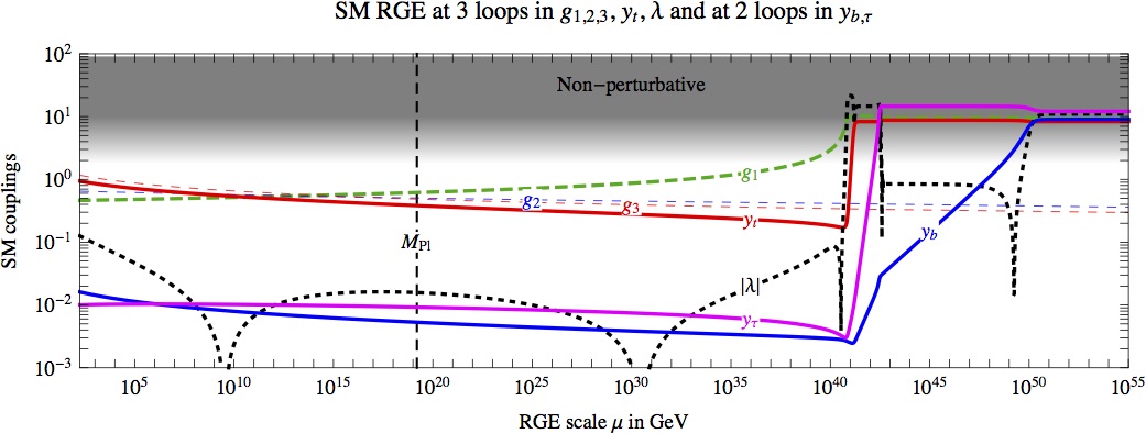
Figure 1: Illustration of a possible RGE running in the SM. We assumed central values for all parameters, and solved the 3 loop RGE equations. In order to obtain an asymptotically safe behaviour we artificially removed the bottom and tau Yukawa contributions to the 3-loop term in the RGE. This only affects the running in the non-perturbative region above $10^{40}\,{\rm GeV}$, where the result cannot of course be trusted. Furthermore we ignored the Yukawa couplings of the lighter generations, and gravity.

One possibility is that the SM is (part of) a theory valid up to infinite energy, such that no physical cut-off exists. Then, once that eq. (2) is interpreted to mean zero, the same divergence in eq. (1) must be interpreted in the same way. Furthermore, in a theory with dimension-less parameters only, one can argue that $\int d^{4}k/k^{2}=0$ by dimensional analysis. Gravity itself could be described by small dimension-less parameters [2, 3], such that it makes sense to extrapolate the SM RGE above the Planck scale.

In this context, one possibility is devising realistic weak-scale extensions of the SM such that all gauge, Yukawa, and quartic couplings flow to zero at infinite energy [3]. However hypercharge must be embedded into a large non-abelian group, in order to be asymptotically free: naturalness then demands new vectors at the weak scale, which have not been observed so far.

The other possibility is that the SM itself might be asymptotically safe. The hypercharge gauge coupling $g_{Y}$ becomes non-perturbative at $\Lambda\sim 10^{40}\,{\rm GeV}$, hitting a ‘Landau pole’. It is not known what it means. It might mean that the SM is not a complete theory and new physics is needed at lower energy. Otherwise $g_{Y}$ and other couplings might run up to constant non-perturbative values as illustrated in fig. 1, such that the SM enters into an asymptotically safe phase. In fact, this possibility was envisioned very early on in the literature [4, 5] triggering lattice studies [6, 7, 8] as well as non-perturbative analytic studies such as the one of [9]. It is fair to say, however, that the fate of the SM depends on non-perturbative effects which are presently unknown; see [10, 11, 12, 13, 14, 15] for attempts to compute the non-perturbative region and for related ideas.

Tavares, Schmaltz and Skiba [16] proposed an alleged no-go argument, according to which Landau makes Higgs obese: i.e. scalars generally receive a mass correction of the order of the would-be-Landau pole scale $\Lambda$. In the SM case, this would mean that, whatever happens at $10^{40}\,{\rm GeV}$, the Higgs mass receives a contribution of order $10^{40}\,{\rm GeV}$, so that an asymptotically safe Higgs (where asymptotic safety kicks above $\Lambda$) cannot be natural.

Later, Litim and Sannino (LS) [17] presented the first four-dimensional example of a perturbative quantum field theory where all couplings that are small at low energy flow to a constant value at higher energy persisting up to infinite energy. This model involves a gauge group $\,{\rm SU}(N_{c})$ with large $N_{c}$, a neutral scalar $S$ and vector-like charged fermions, with asymptotically safe Yukawa couplings and scalar quartics. The model realises Total Asymptotic Safety (TAS). Another equally relevant property of the model is that without the scalar it cannot be perturbatively safe [18, 17]. Scalars are required to dynamically render the theory fundamental at all scales without invoking supersymmetry, which would keep scalars massless independently of their dynamics. In fact supersymmetry makes it harder to realise an asymptotically safe scenario [26, 27] both perturbatively and non-perturbatively. Furthermore the LS model, on the line of physics, connects two fixed points, a non-interacting infrared free one (the theory at low energy is non-abelian QED-like) to an interacting ultraviolet fixed point. Remarkably the model shares the SM backbone since it features gauge, fermion and needed scalar degrees of freedom, albeit it still misses a gauged Higgs-like state. We therefore extend the LS model in section 2 to further feature a Higgs-like charged scalar $H$. We rigorously demonstrate that the theory enters a perturbative asymptotically safe regime at energies above a physical scale $\Lambda$. We also show that we can determine the RGE flow linking ultraviolet and infrared physics precisely.

In the appendix we explore theories featuring chiral fermions and show that it is possible to achieve asymptotic safety for the gauge and Yukawa couplings while safety for scalar couplings is challenging.

Having at our disposal a calculable model similar to the SM, we carefully re-consider the naturalness issue in this class of theories in order to offer an answer to the question: Does the Higgs-like scalar $H$ acquire a mass of the order of the scale $\Lambda$? In section 3 we do not find any such contribution, de facto, re-opening the issue. We discuss possible caveats and offer our conclusions in section 4.

2 Asymptotically safe models with an Higgs-like scalar

Litim and Sannino considered a model with gauge group $\,{\rm SU}(N_{c})$ and gauge coupling $g$; $N_{F}$ vector-like fermions $\psi_{i}\oplus\bar{\psi}_{i}$ in the fundamental plus anti-fundamental, and $N_{F}^{2}$ neutral scalars $S_{ij}$ with Yukawa couplings $S_{ij}\psi_{i}\bar{\psi}_{j}$. The number of flavours $N_{F}$ can be fixed to make the one-loop gauge beta function $\beta_{g}^{(1)}$ small. Large $N_{c}$, $N_{F}$ allows to make $\beta_{g}^{(1)}$ arbitrarily small, guaranteeing perturbative control. The new key feature with respect to the analogous construction by Banks and Zaks [28] is that the Yukawa couplings can (non trivially) make the two-loop gauge beta function negative , such that, together with $\beta_{g}^{(1)}>0$, $g$ enters into a perturbative fixed point at large energy. Finally, one verifies that Yukawa couplings and scalar quartics too have a perturbative fixed point. The model satisfies Total Asymptotic Safety (TAS).

In general the equations $\beta_{g}=\beta_{y}=\beta_{\lambda}=0$ have multiple solutions, that correspond to different global symmetries of the theory. The analysis can be simplified focusing on the maximal global symmetry, $\,{\rm U}(N_{F})_{L}\otimes\,{\rm U}(N_{F})_{R}$, which can be realized with complex scalars $S$. The field content is then summarized by the upper box of table 1.

$$\begin{array}[]{|c|cc|cc|}\hline\cr\hbox{Fields}&\lx@intercol\hfil\hbox{Gauge symmetries}\hfil\lx@intercol\vrule\lx@intercol&\lx@intercol\hfil\hbox{Global symmetries}\hfil\lx@intercol\vrule\lx@intercol\\ \hline\cr&\hbox{Spin}&\,{\rm SU}(N_{c})&\,{\rm U}(N_{F})_{L}&\,{\rm U}(N_{F})_{R}\\ \hline\cr\hline\cr\psi&1/2&{\tiny\yng(1)}&\overline{\tiny\yng(1)}&1\\ \bar{\psi}&1/2&\overline{\tiny\yng(1)}&1&{\tiny\yng(1)}\\ S&0&1&{\tiny\yng(1)}&\overline{\tiny\yng(1)}\\ \hline\cr\hline\cr H&0&{\tiny\yng(1)}&1&1\\ N&1/2&1&1&\overline{\tiny\yng(1)}\\ N^{\prime}&1/2&1&{\tiny\yng(1)}&1\\ \hline\cr\end{array}$$

Table 1: Field content of the model. The upper box is the original Litim-Sannino model. The lower box are the extra fields that we add in order to get a Higgs-like scalar $H$.

The lower box of table 1 shows the fields that we add: one Higgs-like scalar charged under the gauge group. Its introduction does not affect, in the limit of large $N_{c}$, $N_{F}$, the fixed point for $y$ and $g$ found in [17]. We also add singlet fermions $N_{i}$, $N^{\prime}_{i}$ (see table 1 for the details) in order to allow $H$ to have Yukawa couplings, like the SM Higgs. The allowed Yukawa couplings then are

$$\mathscr{L}_{Y}=y\,S_{ij}\psi_{i}\bar{\psi}_{j}+y^{\prime}\,S_{ij}^{*}N_{i}N^{\prime}_{j}+\tilde{y}\,H\bar{\psi}_{i}N_{i}+\tilde{y}^{\prime}\,H^{*}\psi_{i}N^{\prime}_{i}+{\rm h.c.}$$ (3)

The scalar potential is

$$V=\lambda_{S1}(\!\,{\rm Tr}S^{\dagger}S)^{2}+\lambda_{S2}\,{\rm Tr}(S^{\dagger}SS^{\dagger}S)+\lambda_{H}(H^{\dagger}H)^{2}+\lambda_{HS}(H^{\dagger}H)\,{\rm Tr}(SS^{\dagger})\,,$$ (4)

and it is positive if

$$\lambda_{S1}+\eta\lambda_{S2}\geq 0\,,\quad\lambda_{H}>0\,,\quad\lambda_{HS}+2\sqrt{\lambda_{H}(\lambda_{S1}+\eta\lambda_{S2})}\geq 0\,,$$ (5)

where $\eta=\,{\rm Tr}(S^{\dagger}SS^{\dagger}S)/\,{\rm Tr}^{2}(S^{\dagger}S)$ ranges between $\eta=1$ and $\eta=1/N_{F}$. The bounds in eq. (5) need only to be imposed at the extremal values.

2.1 RGE and their fixed points

Defining the $\beta$-functions coefficients as

$$\frac{dX}{d\ln\mu}=\frac{\beta_{X}^{(1)}}{(4\pi)^{2}}+\frac{\beta_{X}^{(2)}}{(4\pi)^{4}}+\dots\,,$$ (6)

the relevant RGE are

$$\halign to=0.0pt{\@eqnsel\hskip\@centering$\displaystyle{#}$&\global\@eqcnt\@ne\hskip 2\arraycolsep\hfil${#}$\hfil& \global\@eqcnt\tw@\hskip 2\arraycolsep$\displaystyle{#}$\hfil&\llap{#}\cr 0.0pt plus 1000.0pt$\displaystyle{\beta_{g}^{(1)} &10.0pt\hfil${=&10.0pt$\displaystyle{g^{3} \left(-\frac{11 }{3}N_{c} +\frac{2 N_{F}}{3}+\frac{1}{6}\right) \\ \beta_{g}^{(2)} &\hbox to0.0pt{\hss=&g^{5}\left(\frac{13N_{c}N_{F}}{3}-\frac{N_{F}}{N_{c}}-\frac{34N_{c}^{2}}{3}+\frac{4N_{c}}{3}-\frac{1}{N_{c}}\right)-g^{3}\left(N_{F}^{2}y^{2}+N_{F}\frac{\tilde{y}^{2}+\tilde{y}^{\prime 2}}{2}\right)\\\beta_{y}^{(1)}&=&y^{3}\left(N_{c}+N_{F}\right)+g^{2}y\left(\frac{3}{N_{c}}-3N_{c}\right)+y\frac{\tilde{y}^{2}+\tilde{y}^{\prime 2}}{2}+yy^{\prime 2}+2y^{\prime}\tilde{y}\tilde{y}^{\prime}\\\beta_{y^{\prime}}^{(1)}&=&N_{c}y^{2}y^{\prime}+y^{\prime 3}(N_{F}+1)+y^{\prime}N_{c}\frac{\tilde{y}^{2}+\tilde{y}^{\prime 2}}{2}+2N_{c}y\tilde{y}\tilde{y}^{\prime}\\\beta_{\tilde{y}}^{(1)}&=&N_{F}\tilde{y}\frac{y^{2}+y^{\prime 2}+2\tilde{y}^{\prime 2}}{2}+\tilde{y}^{3}\left(\frac{N_{c}}{2}+N_{F}+\frac{1}{2}\right)+g^{2}\tilde{y}\frac{3}{2}\frac{1-N_{c}^{2}}{N_{c}}+2N_{F}yy^{\prime}\tilde{y}^{\prime}\\\beta_{\tilde{y}^{\prime}}^{(1)}&=&N_{F}\tilde{y}^{\prime}\frac{y^{2}+y^{\prime 2}+2\tilde{y}^{2}}{2}+\tilde{y}^{\prime 3}\left(\frac{N_{c}}{2}+N_{F}+\frac{1}{2}\right)+g^{2}\tilde{y}^{\prime}\frac{3}{2}\frac{1-N_{c}^{2}}{N_{c}}+2N_{F}yy^{\prime}\tilde{y}\\\beta_{\lambda_{S1}}^{(1)}&=&4y^{2}N_{c}\lambda_{{S1}}+4y^{\prime 2}\lambda_{{S1}}+N_{c}\lambda_{{HS}}^{2}+\left(4N_{F}^{2}+16\right)\lambda_{{S1}}^{2}+16N_{F}\lambda_{{S1}}\lambda_{{S2}}+12\lambda_{{S2}}^{2}\\\beta_{\lambda_{S2}}^{(1)}&=&4y^{2}N_{c}\lambda_{{S2}}-2y^{4}N_{c}+8N_{F}\lambda_{{S2}}^{2}+24\lambda_{{S1}}\lambda_{{S2}}-2y^{\prime 4}+4y^{\prime 2}\lambda_{S2}\\\beta_{\lambda_{H}}^{(1)}&=&g^{4}\left(\frac{3N_{c}}{4}-\frac{3}{N_{c}}+\frac{3}{2N_{c}^{2}}+\frac{3}{4}\right)+g^{2}\left(\frac{6}{N_{c}}-6N_{c}\right)\lambda_{{H}}+\left(4N_{c}+16\right)\lambda_{{H}}^{2}+\\&&+4N_{F}\lambda_{{H}}(\tilde{y}^{2}+\tilde{y}^{\prime 2})+N_{F}^{2}\lambda_{{HS}}^{2}-2N_{F}(\tilde{y}^{4}+\tilde{y}^{\prime 4})\\\beta_{\lambda_{HS}}^{(1)}&=&2(y^{2}N_{c}+y^{\prime 2})\lambda_{{HS}}+(\tilde{y}^{2}+\tilde{y}^{\prime 2})\left(2N_{F}\lambda_{{HS}}-4y^{2}-4y^{\prime 2}\right)+g^{2}\lambda_{{HS}}\left(\frac{3}{N_{c}}-3N_{c}\right)+\\&&+\left(4N_{c}+4\right)\lambda_{{H}}\lambda_{{HS}}+\lambda_{{HS}}\left(\left(4N_{F}^{2}+4\right)\lambda_{{S1}}+8N_{F}\lambda_{{S2}}\right)+4\lambda_{{HS}}^{2}-8yy^{\prime}\tilde{y}\tilde{y}^{\prime}&(7)\cr}}}}}$$

Notice that $yy^{\prime}\tilde{y}^{*}\tilde{y}^{\prime*}$ is left invariant by redefinitions of the phases of all fields, so the model admits one CP-violating phase. Nevertheless CP is conserved at all fixed points, so that the RGE can be written in terms of real couplings. For simplicity we therefore assume all couplings to be real.

The one-loop gauge beta function can be rewritten as

$$\beta_{g}^{(1)}=g^{3}\frac{2N_{c}}{3}\epsilon,\qquad\hbox{where}\qquad\epsilon\equiv\frac{N_{F}}{N_{c}}-\frac{11}{2}+\frac{1}{4N_{c}}$$ (8)

can be made arbitrarily small in the limit of large $N_{c},N_{F}$. In this limit $\beta_{y}^{(1)}$ reduces to

$$\beta_{y}^{(1)}\stackrel{{\scriptstyle N_{c}\gg 1}}{{\simeq}}N_{c}y\bigg{(}-3g^{2}+\frac{13}{2}y^{2}\bigg{)}$$ (9)

and it vanishes for $y^{2}/g^{2}\simeq 6/13$, which corresponds to a negative

$$\beta_{g}^{(2)}{\simeq}\frac{25}{2}g^{5}N_{c}^{2}\bigg{(}1-\frac{363}{325}\bigg{)}.$$ (10)

Thereby the gauge coupling has an IR-attractive fixed point $g=0$ and a non-trivial UV-attractive fixed point at

$$g^{2}=g_{*}^{2}\simeq\frac{26(4\pi)^{2}}{57N_{c}}\epsilon\,.$$ (11)

The scalar quartics $\lambda_{S1},\lambda_{S2}$ admit two fixed points. At leading order in $\epsilon$:

$$\halign to=0.0pt{\@eqnsel\hskip\@centering$\displaystyle{#}$&\global\@eqcnt\@ne\hskip 2\arraycolsep\hfil${#}$\hfil& \global\@eqcnt\tw@\hskip 2\arraycolsep$\displaystyle{#}$\hfil&\llap{#}\cr 0.0pt plus 1000.0pt$\displaystyle{\frac{\lambda_{S1}}{g^{2}} &10.0pt\hfil${\simeq&10.0pt$\displaystyle{\frac{3}{143 N_{F}} \left(- 2 \sqrt{23} \pm\sqrt{20 + 6 \sqrt{23}} \right) \approx-\frac{1}{N_{F}}\left\{\begin{array}[]{ll}0.348&-\\ 0.055&+\end{array}\right.\\ \frac{\lambda_{S2}}{g^{2}} &\hbox to0.0pt{\hss\simeq&\frac{3}{143}\left(\sqrt{23}-1\right)\approx 0.080.&(12)\cr}}}}}$$

The solution with the $+$ ($-$) sign corresponds to a stable (unstable) potential $V(S)$ as determined in [30]. At the stable solution, the fixed point for both quartics, as well as the fixed point for $y$, are IR-attractive: this means that their low-energy values are univocally fixed, with respect to $g$, along the RGE trajectory that reaches infinite energy.

$y/g$	$N_{F}\lambda_{S1}/g^{2}$	$\lambda_{S2}/g^{2}$	$\tilde{y}/g$	$y^{\prime},\tilde{y}^{\prime}/g$	$\lambda_{H}/g^{2}$	$N_{F}\lambda_{HS}/g^{2}$	$V$
$\sqrt{\frac{6}{13}}{\color[rgb]{1,0,0}{}_{\rm IR}}$	$-0.348{\color[rgb]{0,0,1}{}_{\rm UV}}$	$0.080{\color[rgb]{1,0,0}{}_{\rm IR}}$	$0{\color[rgb]{0,0,1}{}_{\rm UV}}$	$0{\color[rgb]{0,0,1}{}_{\rm UV}}$	$0.138{\color[rgb]{0,0,1}{}_{\rm UV}}$	$0{\color[rgb]{0,0,1}{}_{\rm UV}}$	unstable
					$1.362{\color[rgb]{1,0,0}{}_{\rm IR}}$	$0{\color[rgb]{0,0,1}{}_{\rm UV}}$	unstable
			$1/\sqrt{26}{\color[rgb]{1,0,0}{}_{\rm IR}}$	$0{\color[rgb]{0,0,1}{}_{\rm UV}}$	$0.163{\color[rgb]{0,0,1}{}_{\rm UV}}$	$-0.076{\color[rgb]{0,0,1}{}_{\rm UV}}$	unstable
					$1.125{\color[rgb]{1,0,0}{}_{\rm IR}}$	$-0.301{\color[rgb]{0,0,1}{}_{\rm UV}}$	unstable
	$-0.055{\color[rgb]{1,0,0}{}_{\rm IR}}$	$0.080{\color[rgb]{1,0,0}{}_{\rm IR}}$	$0{\color[rgb]{0,0,1}{}_{\rm UV}}$	$0{\color[rgb]{0,0,1}{}_{\rm UV}}$	$0.138{\color[rgb]{0,0,1}{}_{\rm UV}}$	$0{\color[rgb]{1,0,0}{}_{\rm IR}}$	$\geq 0$
					$1.362{\color[rgb]{1,0,0}{}_{\rm IR}}$	$0{\color[rgb]{1,0,0}{}_{\rm IR}}$	$\geq 0$
			$1/\sqrt{26}{\color[rgb]{1,0,0}{}_{\rm IR}}$	$0{\color[rgb]{0,0,1}{}_{\rm UV}}$	$0.163{\color[rgb]{0,0,1}{}_{\rm UV}}$	$0.301{\color[rgb]{1,0,0}{}_{\rm IR}}$	$\geq 0$
					$1.125{\color[rgb]{1,0,0}{}_{\rm IR}}$	$0.076{\color[rgb]{1,0,0}{}_{\rm IR}}$	$\geq 0$

Table 2: Fixed points at leading order in $\epsilon$. The left panel of the table refers to the Litim-Sannino model; the right panel to the extra couplings. All fixed points have $g={g_{*}}{\color[rgb]{0,0,1}{}_{\rm UV}}$, and the extra trivial fixed point with $g=0{\color[rgb]{1,0,0}{}_{\rm IR}}$ is ignored. The pedix _UV denotes an UV-attractive fixed point; while _IR denotes an IR-attractive fixed point, where the low-energy value of the coupling is fixed. The equivalent solutions with $\tilde{y}$, $\tilde{y}^{\prime}$ exchanged are not shown.

So far the new fields that we added just acted as spectators. We must check that they have their own fixed points. By studying the full equations we find that the extra Yukawa couplings $y^{\prime},\tilde{y}$ and $\tilde{y}^{\prime}$ have 3 inequivalent fixed points. The fixed points with $y^{\prime}=\tilde{y}^{\prime}=0$ lead to fixed points for the quartics, as listed in table 2. The full potential $V(S,H)$ is stable when $V(S)$ is stable.

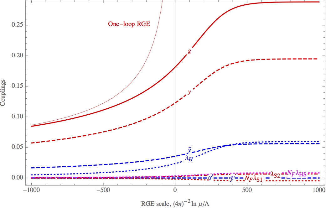
Figure 2: Illustration of a possible RGE running with $N_{c}=10$, $\epsilon=0.01$.

All these couplings are perturbative for $\epsilon\ll 1$, in the sense that higher order corrections are suppressed by powers of $\epsilon$. An explicit solution to the RGE equations is obtained by assuming that all ratios $y/g$, $\lambda/g^{2}$ run remaining constant up to corrections of relative order $\epsilon$. Then one obtains an RGE equation for $g$

$$\frac{dg}{d\ln\mu}\stackrel{{\scriptstyle\epsilon\to 0}}{{\simeq}}\frac{b_{1}g^{3}}{(4\pi)^{2}}-\frac{b_{2}g^{5}}{(4\pi)^{4}},\qquad b_{1}=\frac{2N_{c}}{3}\epsilon,\qquad b_{2}=\frac{19N_{c}^{2}}{13}.$$ (13)

Its solution is

$$\ln\frac{\mu}{\Lambda}=-\frac{(4\pi)^{2}}{2b_{1}}\bigg{[}\frac{1}{g^{2}}+\frac{1}{g_{*}^{2}}\ln\bigg{(}(4\pi)^{2}b_{1}\left(\frac{1}{g^{2}}-\frac{1}{g_{*}^{2}}\right)\bigg{)}\bigg{]},\qquad g^{2}_{*}=(4\pi)^{2}\frac{b_{1}}{b_{2}}.$$ (14)

which can be used to define in an RGE-invariant way the transmutation scale $\Lambda$ in terms of $\mu$ and of $g(\mu)$. In the limit where the second two-loop term is neglected, $\Lambda$ becomes the Landau pole scale of one-loop RGE. Imposing the boundary condition $g(\mu_{0})=g_{0}$ the solution becomes [17]

$$g^{2}(\mu)=\frac{g^{2}_{*}}{1+W[({\mu_{0}}/{\mu})^{2b_{1}^{2}/b_{2}}(g_{*}^{2}/g_{0}^{2}-1)e^{g_{*}^{2}/g_{0}^{2}-1}]}$$ (15)

where $W(z)$ is the Lambert function defined by $z=We^{W}$. The fixed point $g=g_{*}$ is UV-attractive: this means that $g$ can become smaller at low energy. Fig. 2 illustrates a typical RGE running.

3 On the lightness of safe scalars

We now investigate whether scalars can be lighter than the characteristic energy scale $\Lambda$ where the RG flow displays a cross-over from the Gaussian IR scaling to the UV interacting scaling. This scale is dynamical in nature and arises via dimensional transmutation. Above this scale the theory remains finite at arbitrary short distances avoiding the Landau pole. The precise definition and way to determine this scale is presented in [30].

The authors of [16] argued that scalars acquire masses of order $\Lambda$ by elevating a one-loop computation of the top corrections for the SM Higgs to an operatorial one in an alleged theory featuring an asymptotically safe behaviour. Their rough analysis used: dimensional analysis, modelling the underlying behaviour of the couplings and ad-hoc subtractions to render the result finite. Henceforth according to their result the asymptotically safe Higgs scenario would remain unnatural.

Differently from [16] we have the precisely calculable model of section 2, containing a scalar $H$ analogous to the Higgs doublet in the SM, with gauge, Yukawa and quartic interactions, that run into a perturbative ultraviolet fixed point as illustrated in fig. 2. Furthermore the theory connects to a Gaussian IR fixed point. We set all masses to zero, making the classical theory scale invariant, and we determine whether quantum corrections make scalars massive. We perform our computations in such a way that both IR and UV quantum conformality are preserved.

3.1 Perturbative effects

We start by considering the quantum corrections affecting scalar masses that stem from the standard perturbative approach of summing Feynman diagrams. We therefore fix the renormalisation scale at an arbitrary value $\mu_{0}$, and compute the scalar two-point function $\Pi(0)$. At any loop order, each diagram is proportional to powers of dimension-less coupling constants renormalized at $\mu_{0}$ times a loop integral which is scale-invariant and quadratically divergent at large loop momenta. To ensure short and large distance quantum conformality these divergences are set to zero. As well known, scale-invariant loop integrals vanish automatically in dimensional regularisation.

3.2 Resumming large logarithms, $\Lambda$ dependence and meaning

One might be worried that a mere perturbative analysis is insufficient to settle the issue. So, we now comment on potentially different non-perturbative corrections.

A relevant class of dominant non-perturbative corrections are those where couplings get enhanced by large logarithms. At one loop one encounters corrections of relative order $C\ell$ where $C=N_{c}g^{2}/(4\pi)^{2}$ and $\ell=\ln(E/\mu_{0})$. The correction $C\ell$ becomes of order one at energy $E$ much different from $\mu_{0}$. At two loops one encounters corrections of order $C^{2}\ell^{2}$ and $C^{2}\ell$.

As well known, all corrections of order $(C\ell)^{n}$ can be resummed by solving the one-loop RGE equations; all corrections of order $C^{n}\ell^{n-1}$ are resummed by solving the two-loop RGE equations, and so on. The RGE equations $know$ that $\Lambda$ is a special scale. In order to compute whether scalar masses receive corrections of order $\Lambda$, we must compute and solve the RGE equations for massive parameters. The RGE for squared scalar masses have the following generic form, dictated by dimensional analysis:

$$\frac{d}{d\ln\mu}{m}^{2}=\hbox{(dimension-less couplings)}\times{m}^{2}.$$ (16)

The right-handed side in general contains scalar masses, fermion masses and cubic scalar couplings. Without explicit computations it is clear that, if we set all masses to zero at any scale $\mu_{0}$ (for example a scale much above $\Lambda$), all masses will remain zero at any other scale $\mu$ (for example a scale much below $\Lambda$). No scalar mass of order $\Lambda$ is generated trough RGE evolution when the $\Lambda$ threshold is crossed.

In fact the RG-invariant scale $\Lambda$ appears when solving for the RG equations. In models with a single scalar squared mass one has:

$$\frac{m^{2}(\mu)}{m^{2}(\mu_{0})}=\exp\left[\int_{\mu_{0}}^{\mu}\left(\Delta_{m^{2}}-2\right)\,d\ln\mu\right]\ ,$$ (17)

with

$$\frac{\beta_{m^{2}}}{m^{2}(4\pi)^{2}}=\frac{d\ln m^{2}}{d\ln\mu}=\Delta_{m^{2}}-2\ .$$ (18)

Here $\Delta_{m^{2}}$ is the quantum dimension of the mass operator. The non-trivial $\Lambda$ dependence is automatically encoded in the running of the various couplings entering in the above expression. While $\Lambda$-dependent, the renormalisation of $m^{2}$ is multiplicative: the additive renormalisation of order $\Lambda^{2}$ claimed in [16] is absent. This shows that these type of corrections do not introduce an explicit mass-term for the scalars despite the presence of an RG-invariant $\Lambda$. In addition, according to our interpretation of the scale $\Lambda$ no special scheme is privileged.

The ratio $m/\Lambda$ allows to measure deviations from IR quantum conformality when making the arbitrary choice of the bare mass of the scalar, or any other physical scale. Near IR quantum conformality can, in fact, be naturally ensured in the present framework requiring $m\ll\Lambda$ for any $\mu<\Lambda$. In other words we use $\Lambda$ as the RG-invariant meter to compare scales.

In order to make the discussion more explicit, we consider the model of section 2 and determine the RGE for the mass term operators $m_{H}^{2}|H|^{2}+m_{S}^{2}|S|^{2}$ that would explicitly break scale symmetry (fermion masses still vanish because of the chiral symmetry). Their one-loop RGE are:

$$\beta_{m_{H}^{2}}^{(1)} =m_{H}^{2}\left[g^{2}\left(\frac{3}{N_{c}}-3N_{c}\right)+4\lambda_{H}(N_{c}+1)+2N_{F}\tilde{y}^{2}+2N_{F}\tilde{y}^{\prime 2}\right]+2m_{S}^{2}\lambda_{HS}N_{F}^{2},$$ (19)

$$\beta_{m_{S}^{2}}^{(1)} =m_{S}^{2}\left[4\lambda_{S1}\left(N_{F}^{2}+1\right)+8\lambda_{S2}N_{F}+2N_{c}y^{2}+2{y^{\prime 2}}\right]+2m_{H}^{2}\lambda_{HS}N_{c}.$$ (20)

The couplings evolve satisfying $g^{2}\propto y^{2}\propto\lambda$ to leading order in $\epsilon$ along the UV-attractive asymptotically-safe trajectory connecting the theory to the IR Gaussian fixed point. So the RGE for the masses reduce to independent equations for appropriate linear combinations $m^{2}_{i}$ of the squared masses. Neglecting sub-leading terms in the limit of large $N_{c},N_{F}$ the RGE for $m_{S}^{2}$ depends only on itself:

$$\beta^{(1)}_{m^{2}_{S}}=\frac{6}{13}\sqrt{20+6\sqrt{23}}\,\cdot{g^{2}N_{c}}m_{S}^{2}.$$ (21)

Eq. (21) can be integrated analytically, giving

$$\frac{m_{S}^{2}(\mu)}{m_{S}^{2}(\mu_{0})}=w^{\frac{4\epsilon}{19}\sqrt{20+6\sqrt{23}}}\qquad\hbox{where}\qquad w=\bigg{[}\frac{1-g_{*}^{2}/g^{2}(\mu)}{1-g_{*}^{2}/g^{2}(\mu_{0})}\bigg{]}^{-\frac{171}{104\epsilon^{2}}}.$$ (22)

Considering the fixed point with $\tilde{y},\lambda_{HS}\neq 0$, and defining the numerical constants $\bar{\lambda}_{H}=\lambda_{H}/g^{2}$ and $\bar{\lambda}_{HS}=N_{F}\lambda_{HS}/g^{2}$ listed in table 2, eq. (19) can also be integrated and gives

$$\frac{m_{H}^{2}(\mu)}{m^{2}_{H}(\mu_{0})}=w^{-\frac{\epsilon}{57}(67-104\bar{\lambda}_{H})}+\frac{286\bar{\lambda}_{HS}\,m_{S}^{2}(\mu_{0})/m^{2}_{H}(\mu_{0})}{67+12\sqrt{20+6\sqrt{23}}-104\bar{\lambda}_{H}}\left(w^{\frac{4\epsilon}{19}\sqrt{20+6\sqrt{23}}}-w^{-\frac{\epsilon}{57}(67-104\bar{\lambda}_{H})}\right)$$ (23)

The factor $w$ can be explicitly written as ratios of Lambert functions using eq. (15), and at ultra-high energies $\mu,\mu_{0}\gg\Lambda$ it reduces to $w\simeq\mu/\mu_{0}$. The solutions to the RGE in this limit can be easily obtained substituting constant couplings in eq.s (19) and (20). These expressions say that the various massive parameters $m_{i}$ acquire dimension $1+{\cal O}(\epsilon)$ at energies above $\Lambda$. Our results recover the fact that a massive scalar contributes to the mass of other scalars coupled to it. The physical ratios between different masses in general run by an infinite amount up to infinite energy: this can be seen as a motivation for considering theories where all masses vanish, being generated only at low energy trough dynamical generation of vacuum expectation values or condensates. However it does not mean that masses receive power-divergent corrections: no mass is generated trough RGE running, if masses vanish at some scale.

3.3 Non-perturbative contributions

Finally, we discuss now truly non-perturbative effects, which could give corrections of order $\Lambda^{2}e^{-1/C}$. In the model of section 2 the couplings $C$ can be chosen to be arbitrarily small, such that non-perturbative effects, even if present, are exponentially suppressed. In this model there are no new bound states with masses of order $\Lambda$, no condensates of order $\Lambda$, no new non-perturbative phenomena: The RG invariant scale $\Lambda$ merely determines the boundary between the IR and the UV regime.

In order to make the discussion more concrete, we discuss two special cases of non-perturbative phenomena.

First, if the fixed point is not fully IR-attractive the quartics could run to low-energy values that violated the positivity condition of the potential, cross the boundary in eq. (5) at a scale $\mu\sim M$ exponentially smaller than $\Lambda$. If this happens, scalars acquire vacuum expectation values and masses order $M$ trough the Coleman-Weinberg mechanism. Indeed various works proposed extensions of the Standard Model where the weak scale is generated in this way.

Next, we notice that the running of the SM Higgs quartic $\lambda_{H}$ in fig. 1 exhibits a similar, but more complex pattern: there is a $2-3\sigma$ hint that $\lambda_{H}$ runs negative between $E_{\rm min}\sim 10^{10}\,{\rm GeV}$ and $E_{\rm max}\sim 10^{30}\,{\rm GeV}$, see fig. 1. As well known, this implies a vacuum decay rate suppressed by the non-perturbative factor $e^{-S}$, where $S=8\pi^{2}/3|\lambda_{H}(E)|$ is the action of the Fubini bounce $h_{E}(r)=\sqrt{-2/\lambda}\times 2E/(1+E^{2}r^{2})$. Here $r^{2}=x^{2}+y^{2}+z^{2}-t^{2}$ and $E$ is a free parameter with dimension of mass, that arises because of classical scale invariance. The non-perturbative Fubini bounce also leads to a non-perturbative correction to the Higgs mass of order

$$\delta m_{H}^{2}\sim\int_{E_{\rm min}}^{E_{\rm max}}E\,dE~{}e^{-S}.$$ (24)

Such non-perturbative correction to the Higgs mass is negligibly small, given that vacuum decay is negligibly slow comparte to cosmological time-scale, namely $e^{-S}\ll(H_{0}/E)^{4}$ where $H_{0}$ is the Hubble rate.

We conclude this section by asserting that in an asymptotically safe theory featuring Higgs-like states no masses are generated along the trajectory connecting the IR Gaussian fixed point dynamics to the interacting UV safe one. The intrinsic and calculable RG invariant scale $\Lambda$ merely determines the boundary between the IR and UV conformal regimes. Furthermore at this scale no new fundamental degrees of freedom are generated. This is so since the underlying theory is described by the same fundamental degrees of freedom along the entire RG flow. When introducing explicit conformal symmetry breaking operators such as the Higgs mass term the scale $\Lambda$ allows us to ensure that deviations from the IR quantum conformal behaviour are minimal so that the physical mass $m\ll\Lambda$ for any $\mu<\Lambda$. This can be naturally achieved in any UV and IR conformal preserving renormalization scheme.

Our results show that the claim that asymptotically safe scalars are never naturally light [16] maximally violates quantum IR (near) conformality by, de facto, elevating the RG invariant scale $\Lambda$ to the mass scale of the Higgs.

4 Conclusions

In section 2 we extended the Litim-Sannino [17] theory to further contain a Higgs-like scalar $H$ charged under the gauge group and with further Yukawa and quartic interactions. We showed that all couplings are governed by an IR Gaussian fixed point at low energies, and grow at short distance until a scale $\Lambda$. Above this scale the couplings enter into a rigorous asymptotically safe regime up to infinite energy, thereby avoiding Landau poles as illustrated in fig. 2.

In section 3 we investigated the perturbative and non-perturbative quantum corrections to the scalar mass operator. To better elucidate our main points, we determined these corrections for the calculable model of section 2, serving as SM template. We showed that no scalar masses of order of the transmutation scale $\Lambda$ are generated along the entire RG trajectory connecting the IR Gaussian fixed point to the UV interacting fixed point. Scalars which are massless above $\Lambda$ remain massless below $\Lambda$. Only exponentially small non-perturbative corrections can contribute to scalar masses, as discussed in section 3.3. This can be understood trough dimensional analysis, analogously to how we understand that a fermion mass $M$ contributes to a scalar squared mass at order $M^{2}$. In our model interactions give quantum dimensions of order $\epsilon=N_{c}g^{2}/(4\pi)^{2}$, which never gets of order unity because $g$ is perturbative. Thereby many powers are needed to form a squared scalar mass, which can only be generated at non-perturbative order $\epsilon^{2/\epsilon}$. Our couplings can be arbitrarily perturbative: for example a QED-like loop factor of order $\epsilon=1/1000$ corresponds to $\delta m^{2}\sim(1000^{-1000}\Lambda)^{2}$, contrary to [16] who claimed that scalar masses $m^{2}$ unavoidably receive quantum corrections $\delta m^{2}$ of the order of the transmutation scale $\Lambda^{2}$, such that scalars lighter than $\Lambda$ would be unnatural.

If scalar masses are added to the theory, they receive the multiplicative RGE corrections of eq. (17) that have been computed in section 3.2 in the explicit model. These yield a non-trivial and non-quadratic $\Lambda$ dependence arising solely from the dynamics. The mass of Higgs-like scalars can be naturally small relative to the scale $\Lambda$ that acts, in this respect, merely as a comparison scale. Our results do not validate the claims made in [16] that, in practice by the use of ad-hoc regularization schemes, elevated the scale $\Lambda$ to the mass of the Higgs, maximally violating, at least the low energy (near) conformality of the theory. It is worth stressing that, differently from the naive estimates of[16], never in our computations we had to resort to ad-hoc assumptions or expansions around one of the two fixed points since we can rigorously solve for the flow connecting the IR and UV, including the determination of the nontrivial anomalous dimensions. Our results naturally capture the correct power-law behaviour when approaching the UV interacting fixed point as already explained in sections F, G of [17].

Our interest further resides in using these computable models to motivate new avenues for the SM near the scale $\Lambda\sim 10^{40}\,{\rm GeV}$, where the hypercharge coupling $g_{Y}$ nears its Landau pole. To this end a case-by-case investigation is needed. In particular a phenomenologically viable application to the SM case would deserve a proper dedicated study to firmly establish what happens near the hypercharge Landau pole. Do couplings enter into an asymptotically safe regime, as illustrated in fig. 1? If yes, would the Higgs mass remain naturally small, or non-perturbative dynamics generate condensates of order $\Lambda$ that affect the Higgs mass? Our explicit example demonstrates that such a possibility is worth exploring.

Acknowledgements

This work was supported by the grant 669668 – NEO-NAT – ERC-AdG-2014 and the Danish National Research Foundation under the grant DNRF:90. We thank Ara Ioannisian for useful discussions. A.S. thanks Riccardo Rattazzi for discussions about dimensional analysis. Martin Schmaltz is thanked for discussions and clarifications of his work during the 2016 CERN workshop Charting the Unknown.

Appendix A Asymptotically safe models with chiral fermions?

Here we analyse basic models with chiral fermions, partially inspired by the traditional structures of grand unified theories. Our goal is not to be exhaustive but rather to guide the reader towards these extensions while exemplifying the challenges one faces in building TAS extensions of this kind. In particular we add one or more families of chiral fermions. The minimal chiral anomaly-free family is made of either one anti-symmetric $\psi_{A}$ and $N_{c}-4$ anti-fundamentals $\tilde{\psi}$ or of one symmetric $\psi_{S}$ and $N_{c}+4$ anti-fundamentals $\tilde{\psi}$ of $\,{\rm SU}(N_{c})$. The two possibilities coincide in the limit of large $N_{c}$, where no other possibility exists: all higher representations of $\,{\rm SU}(N_{c})$ with 3 or more indeces contribute to $\beta_{g}^{(1)}$ more than vectors at large $N_{c}$, such that $\beta_{g}^{(1)}$ becomes large and positive. Spinors of $\,{\rm SO}(N_{c})$ have the same problem: $\beta_{g}^{(1)}$ cannot be small.

A look at the relevant $\,{\rm SU}(N_{c})$ group-theorethical factors

$$\begin{array}[]{c|ccc}\hbox{representation}~{}R&\hbox{dimension }d_{R}&T_{R}\hbox{ in $\,{\rm Tr}(T^{a}T^{b})=T_{R}\delta^{ab}$}&C_{R}=d_{G}T_{R}/d_{R}\\ \hline\cr\hbox{singlet}&1&0&0\\ \hbox{fundamental}&N_{c}&1/2&N_{c}/2-1/2N_{c}\\ \hbox{adjoint}&N_{c}^{2}-1&N_{c}&N_{c}\\ \hbox{anti-symmetric}&N_{c}(N_{c}-1)/2&(N_{c}-2)/2&N_{c}-1-2/N_{c}\\ \hbox{symmetric}&N_{c}(N_{c}+1)/2&(N_{c}+2)/2&N_{c}+1-2/N_{c}\\ \end{array}$$ (25)

shows that adding minimal chiral fermions cannot be a correction which is sub-leading in the limit of large $N_{c}$ with respect to the LS model. A non-trivial feature of this model is that the Yukawa contribution makes $\beta_{g}^{(2)}=\beta_{g}^{(2)}|_{\rm gauge}+\beta_{g}^{(2)}|_{\rm Yukawa}$ negative.

In general, it is not easy to satisfy this crucial condition. The generic expressions for the gauge beta functions

$$\halign to=0.0pt{\@eqnsel\hskip\@centering$\displaystyle{#}$&\global\@eqcnt\@ne\hskip 2\arraycolsep\hfil${#}$\hfil& \global\@eqcnt\tw@\hskip 2\arraycolsep$\displaystyle{#}$\hfil&\llap{#}\cr 0.0pt plus 1000.0pt$\displaystyle{\beta_{g}^{(1)} &10.0pt\hfil${=&10.0pt$\displaystyle{g^{3} \bigg{[}-\frac{11}{3} C_{G} + {\sum_{F}} \frac{2}{3} T_{F} + {\sum_{S} \kappa_{S} \frac{1}{3}} T_{S}\bigg{]},\\ \beta_{g}^{(2)} |_{\rm gauge} &\hbox to0.0pt{\hss=&g^{5}\bigg{[}-\frac{34}{3}C_{G}^{2}+\sum_{F}\bigg{(}2C_{F}+\frac{10}{3}C_{G}\bigg{)}T_{F}+{\sum_{S}\kappa_{S}}\bigg{(}{4}C_{S}+\frac{{2}}{3}C_{G}\bigg{)}T_{S}\bigg{]}\,,&(26)\cr}}}}}$$

(where $\kappa_{S}=1,\,1/2$ for complex or real scalars respectively) show that, choosing a matter content such that $\beta_{g}^{(1)}=0$, $\beta_{g}^{(2)}|_{\rm gauge}$ is positive and minimal if the matter content consists only of fermions in the fundamental, as in the LS model, where the total $\beta_{g}^{(2)}$ is negative by a relatively small amount, see eq. (10). Adding one or more chiral families and a small number ($\ll N_{c}\sim N_{F}$) of Higgs scalars in the fundamental coupled to the fermions as $H^{*}\tilde{\psi}\psi_{A,S}$, we find that the conditions $\beta_{g}^{(1)}=0$ and $\beta_{g}^{(2)}<0$ cannot be satisfied together. No perturbative UV-interacting fixed point can be found for the gauge and yukawa couplings.

We then need to consider more involved models. In general, it is convenient to add as many singlet fermions and/or scalars as possible, as they can allow for extra Yukawa couplings contributing to a negative $\beta_{g}^{(2)}|_{\rm Yukawa}$ without contributing to $\beta_{g}^{(2)}|_{\rm gauge}$. Indeed the LS model introduces many singlet scalars $S$.

Table 3 shows a model candidate to be Totally Asymptotically Safe, obtained adding one chiral family to the LS model, some Higgs-like scalars $H$ and some neutral scalars $\tilde{S}$. A more complex pattern of Yukawa couplings is allowed, making more complicated to compute their possible fixed points.

$$\begin{array}[]{|c|c|ccc|}\hline\cr\hbox{Fields}&\hbox{Gauge}&\lx@intercol\hfil\hbox{Global symmetries}\hfil\lx@intercol\vrule\lx@intercol\\ \hline\cr&\,{\rm SU}(N_{c})&\,{\rm U}(N_{F})_{L}&\,{\rm U}(N_{F})_{R}&\,{\rm U}(N_{c}\pm 4)\\ \hline\cr\hline\cr\psi&{\tiny\yng(1)}&\overline{\tiny\yng(1)}&1&1\\ \bar{\psi}&\overline{\tiny\yng(1)}&1&{\tiny\yng(1)}&1\\ S&1&{\tiny\yng(1)}&\overline{\tiny\yng(1)}&1\\ \hline\cr\hline\cr\psi_{A,S}&{\tiny\yng(1,1)},{\tiny\yng(2)}&1&1&1\\ \tilde{\psi}&\overline{\tiny\yng(1)}&1&1&{\tiny\yng(1)}\\ \tilde{S}&1&{\tiny\yng(1)}&1&\overline{\tiny\yng(1)}\\ H&{\tiny\yng(1)}&1&1&{\tiny\yng(1)}\\ \hline\cr\end{array}$$

Table 3: A candidate model with anomaly-free chiral fermions $\tilde{\psi}\oplus\psi_{A,S}$ and Higgs-like scalars $H$ that might satisfy Total Asymptotic Safety. As in table 1, the upper box represents the original LS model, while in the lower box are listed the extra fields.

Fixed points correspond to specific values of the couplings such that all their beta-functions vanish. The theories under consideration allow for $\sim N_{c}^{3}$ Yukawa couplings. In a theory with many couplings the equations $\beta=0$ can have many different solutions. Each solution seems to correspond to a specific flavour symmetry, because couplings with the same gauge quantum numbers have the same beta functions. Although we don’t know whether this is a generic mathematical result, we proceed by computing the $\beta$ functions assuming the various possible flavour symmetries, such that the number of independent Yukawa couplings is reduced to a few. For example, the LS model assumed the maximal flavour symmetry allowed by its matter content, see table 1, such that there is only one independent Yukawa coupling $y$. In table 3 we again assume a quasi-maximal flavour symmetry. The most generic Yukawa interactions allowed by the gauge and global flavour symmetries then are

$$\mathscr{L}_{Y}=y_{1}S\psi\bar{\psi}+\tilde{y}_{1}\tilde{S}\psi\tilde{\psi}+\tilde{y}_{2}H^{*}\psi_{A,S}\tilde{\psi}+\hbox{h.c.}$$ (27)

The one-loop RGE for the gauge coupling is

$$\beta^{(1)}_{g}=g^{3}\bigg{[}-\frac{17}{6}N_{c}+\frac{2}{3}N_{F}\pm\frac{8}{3}\bigg{]}=g^{3}\frac{2N_{c}}{3}\epsilon,\qquad\epsilon=\frac{N_{F}\pm 4}{N_{c}}-\frac{17}{4}.$$ (28)

The RGE for the Yukawa couplings in the relevant limit $\epsilon\ll 1$ and $N_{c}\gg 1$ are

$$\left\{\begin{array}[]{l}\beta_{y_{1}}^{(1)}\simeq N_{c}y_{1}[-3g^{2}+\frac{21}{4}y_{1}^{2}+\frac{1}{2}\tilde{y}_{1}^{2}],\\ \beta_{\tilde{y}_{1}}^{(1)}\simeq\frac{1}{4}N_{c}\tilde{y}_{1}[-12g^{2}+\frac{17}{2}y_{1}^{2}+\frac{29}{2}\tilde{y}_{1}^{2}+\tilde{y}_{2}^{2}],\\ \beta_{\tilde{y}_{2}}^{(1)}\simeq\frac{1}{4}N_{c}\tilde{y}_{2}[-18g^{2}+\frac{17}{2}\tilde{y}_{1}^{2}+5\tilde{y}_{2}^{2}].\end{array}\right.$$ (29)

They have a few fixed-point solutions. One solution is

$$y_{1}^{2}=\frac{684}{1259}g^{2},\qquad\tilde{y}_{1}^{2}=\frac{372}{1259}g^{2},\qquad\tilde{y}_{2}^{2}=\frac{3900}{1259}g^{2}.$$ (30)

This fixed point leads to a negative

$$\beta_{g}^{(2)}\stackrel{{\scriptstyle N_{c}\gg 1}}{{\simeq}}\frac{53}{4}g^{5}N_{c}^{2}\bigg{(}1-\frac{67443}{66727}\bigg{)}$$ (31)

such that $g$ has a fixed point, that we compute at leading order in $\epsilon$ and $1/N_{c}$:

$$g_{*}^{2}\simeq\frac{2518}{537}\frac{(4\pi)^{2}}{N_{c}}\epsilon.$$ (32)

Again, $\epsilon$ can be made arbitrarily small, such that $g_{*}$ can be perturbative. The scalar potential that respects the assumed flavour symmetry contains 11 scalar quartics:

$$V = \lambda_{S}\,{\rm Tr}[S^{\dagger}S]^{2}+\lambda_{S}^{\prime}\,{\rm Tr}[S^{\dagger}SS^{\dagger}S]+\lambda_{\tilde{S}}\,{\rm Tr}[\tilde{S}^{\dagger}\tilde{S}]^{2}+\lambda_{\tilde{S}}\,{\rm Tr}[\tilde{S}^{\dagger}\tilde{S}\tilde{S}^{\dagger}\tilde{S}]+$$ (33)

$$+\lambda_{H}(H^{\dagger}H)^{2}+\lambda^{\prime}_{H}\,{\rm Tr}[H^{\dagger}HH^{\dagger}H]+\lambda_{S\tilde{S}}\,{\rm Tr}[S^{\dagger}S]\,{\rm Tr}[\tilde{S}^{\dagger}\tilde{S}]+\lambda^{\prime}_{S\tilde{S}}\,{\rm Tr}[SS^{\dagger}\tilde{S}\tilde{S}^{\dagger}]+$$

$$+\lambda_{HS}\,{\rm Tr}[SS^{\dagger}](H^{\dagger}H)+\lambda_{H\tilde{S}}\,{\rm Tr}[\tilde{S}\tilde{S}^{\dagger}](H^{\dagger}H)+\lambda^{\prime}_{H\tilde{S}}\,{\rm Tr}[\tilde{S}HH^{\dagger}\tilde{S}^{\dagger}]\,.$$

We computed their RGE equations, but we don’t find any fixed point for them. There seems to be no particular reason: just a matter of unlucky order one factors in a system of 11 quadratic equations that would fill a page. Adding extra neutral fermions $N$ transforming as anti-fundamentals of $\,{\rm SU}(N_{F})_{R}\otimes\,{\rm SU}(N_{c}\pm 4)$ and $N^{\prime}$ transforming as fundamentals of $\,{\rm SU}(N_{F})_{L}\otimes\,{\rm SU}(N_{c}\pm 4)$ allows for extra Yukawa couplings analogous to the one in eq. (3); however we cannot find other fixed point solutions for the gauge and yukawa couplings apart from the solution of eq. (30).

We tried to reduce the global symmetries in order to search for more generic fixed points. For example the symmetric and anti-symmetric components of $S$ transform independently under the flavour symmetry $\,{\rm SU}(N_{F})_{V}$, such that $V$ now contains 14 independent quartics. Still, they have no fixed points. Alternatively, the global symmetry $\,{\rm SO}(N_{F})_{L}\otimes\,{\rm U}(N_{F})_{R}\otimes\,{\rm SO}(N_{c}\pm 4)$ is respected if the scalars $\tilde{S}$ are real, changing order one factors in the RGE. The allowed Yukawa couplings

$$\mathscr{L}_{Y}=y_{1}S\psi\bar{\psi}+\frac{\tilde{y}_{1}}{\sqrt{2}}\tilde{S}\psi\tilde{\psi}+\tilde{y}_{2}H^{\dagger}\psi_{S}\tilde{\psi}\,,$$ (34)

have a fixed point

$$y_{1}^{2}=\frac{924}{1679}g^{2},\qquad\tilde{y}_{1}^{2}=\frac{744}{1679}g^{2},\qquad\tilde{y}_{2}^{2}=\frac{5412}{1679}g^{2}\,,$$ (35)

corresponding to a negative $\beta_{g}^{(2)}$. Again, the 13 quartics now allowed by the symmetries do not have any fixed point. Finally, we tried adding extra neutral fermions that allow for extra Yukawa couplings, but this does not have a beneficial effect. We reported the negative results regarding our preliminary analysis of chiral matter to help elucidate the challenges one faces with this class of models but also to guide the reader towards more successful attempts like the ones in section V of [32].

References

- [1] M. Farina, D. Pappadopulo, A. Strumia, “A modified naturalness principle and its experimental tests”, JHEP 1308 (2013) 022 [arXiv:1303.7244].
- [2] A. Salvio, A. Strumia, “Agravity”, JHEP 1406 (2014) 080 [arXiv:1403.4226].
- [3] G.F. Giudice, G. Isidori, A. Salvio, A. Strumia, “Softened Gravity and the Extension of the Standard Model up to Infinite Energy”, JHEP 1502 (2015) 137 [arXiv:1412.2769]. G.M. Pelaggi, A. Strumia, S. Vignali, “Totally asymptotically free trinification”, JHEP 1508 (2015) 130 [arXiv:1507.06848].
- [4] M. Gell-Mann and F. E. Low, “Quantum electrodynamics at small distances ”, Phys. Rev. 95 (1954) 1300.
- [5] S. Weinberg, in C76-07-23.1 HUTP-76/160, Erice Sub-nucl. Phys., 1, (1976).
- [6] M. Gockeler, R. Horsley, V. Linke, P.E.L. Rakow, G. Schierholz, H. Stuben, “Is there a Landau pole problem in QED?”, Phys. Rev. Lett. 80 (1997) 4119 [arXiv:hep-th/9712244].
- [7] S. Kim, J.B. Kogut, M-P. Lombardo, “On the triviality of textbook quantum electrodynamics”, Phys. Lett. B502 (2000) 345 [arXiv:hep-lat/0009029].
- [8] S. Kim, J.B. Kogut, M-P. Lombardo, “Gauged Nambu-Jona-Lasinio studies of the triviality of quantum electrodynamics”, Phys. Rev. D65 (2001) 054015 [arXiv:hep-lat/0112009]
- [9] H. Gies, J. Jaeckel, “Renormalization flow of QED”, Phys. Rev. Lett. 93 (2004) 110405 [arXiv:hep-ph/0405183]
- [10] N.N. Bogoliubov, A.A. Logunov, D.V. Shirkov, “The method of dispersion relations and perturbation theory”, Sov. Phys. JETP 37 (1960) 574.
- [11] P.J. Redmond and J.L. Uretsky, “Conjecture concerning the properties of nonrenormalizable field theories”, Phys. Rev. Lett. 1 (1958) 147 [doi].
- [12] D.V. Shirkov, I.L. Solovtsov, “Analytic model for the QCD running coupling with universal value”, Phys. Rev. Lett. 79 (1997) 1209 [arXiv:hep-ph/9704333].
- [13] I.M. Suslov, “Exact asymptotics for beta-function in QED”, J. Exp. Theor. Phys. 108 (2008) 980 [arXiv:0804.2650].
- [14] I.M. Suslov, “Renormalization Group Functions of the Theory in the Strong Coupling Limit: Analytical Results”, J. Exp. Theor. Phys. 107 (2010) 413 [arXiv:1010.4081].
- [15] G. ’t Hooft, “The Conformal Constraint in Canonical Quantum Gravity” [arXiv:1011.0061]. G. ’t Hooft, “A class of elementary particle models without any adjustable real parameters”, Found. Phys. 41 (2011) 1829 [arXiv:1104.4543].
- [16] G. Marques Tavares, M. Schmaltz, W. Skiba, “Higgs mass naturalness and scale invariance in the UV”, Phys. Rev. D89 (2014) 015009 [arXiv:1308.0025].
- [17] D.F. Litim, F. Sannino, “Asymptotic safety guaranteed”, JHEP 1412 (2014) 178 [arXiv:1406.2337]. See also [30].
- [18] W. E. Caswell, “Asymptotic Behavior of Nonabelian Gauge Theories to Two Loop Order”, Phys. Rev. Lett. 33 (1974) 244.
- [19] M. Aizenman, “Proof of the Triviality of in -Dimensions Field Theory and Some Mean Field Features of Ising Models for ”, Phys. Rev. Lett. 47 (1981) 1.
- [20] J. Frohlich, “On the Triviality of Lambda in -Dimensions Theories and the Approach to the Critical Point in Dimensions ”, Nucl. Phys. B 200 (1982) 281.
- [21] M. Luscher and P. Weisz, “Scaling Laws and Triviality Bounds in the Lattice Theory. 1. One Component Model in the Symmetric Phase”, Nucl. Phys. B 290 (1987) 25.
- [22] M. Luscher and P. Weisz, “Scaling Laws and Triviality Bounds in the Lattice Theory. 2. One Component Model in the Phase with Spontaneous Symmetry Breaking”, Nucl. Phys. B 295 (1988) 65.
- [23] U.M. Heller, M. Klomfass, H. Neuberger, P.M. Vranas, “Regularization dependence of the Higgs mass triviality bound”, Nucl. Phys. Proc. Suppl. 30 (1992) 685 [arXiv:hep-lat/9210026]
- [24] U. Wolff, “Precision check on triviality of theory by a new simulation method”, Phys. Rev. D79 (2009) 105002 [arXiv:0902.3100].
- [25] T. Korzec, U. Wolff, “Triviality of in the broken phase revisited”, PoS LATTICE2014 (2015) 305 [arXiv:1502.03714].
- [26] K. Intriligator, F. Sannino, “Supersymmetric asymptotic safety is not guaranteed”, JHEP 1511 (2015) 023 [arXiv:1508.07411].
- [27] B. Bajc, F. Sannino, “Asymptotically Safe Grand Unification”, JHEP 1612 (2016) 141 [arXiv:1610.09681].
- [28] T. Banks, A. Zaks, “On the phase structure of vector-like gauge theories with massless fermions”, Nucl. Phys. B196 (1982) 189.
- [29] O. Antipin, M. Gillioz, E. Mølgaard, F. Sannino, “The a theorem for gauge-Yukawa theories beyond Banks-Zaks fixed point”, Phys. Rev. D87 (2013) 125017 [arXiv:1303.1525].
- [30] D.F. Litim, M. Mojaza, F. Sannino, “Vacuum stability of asymptotically safe gauge-Yukawa theories”, JHEP 1601 (2016) 081 [arXiv:1501.03061].
- [31] A.D. Bond, D.F. Litim, “Theorems for Asymptotic Safety of Gauge Theories”, Eur. Phys. J. C77 (2017) 429 [arXiv:1608.00519].
- [32] E. Molgaard, F. Sannino, “Asymptotically safe and free chiral theories with and without scalars”, Phys. Rev. D96 (2017) 056004 [arXiv:1610.03130].
- [33] O. Antipin, F. Sannino, “Conformal Window 2.0: The Large Safe Story” [arXiv:1709.02354].
- [34] F. Sannino, plenary talk held for the ERG 2016 meeting in Trieste. The slides of the presentation can be found at this link.