Various Local Heating Events in the Earliest Phase of Flux Emergence

Abstract

Emerging flux regions (EFRs) are known to exhibit various sporadic local heating events in the lower atmosphere. To investigate the characteristics of these events, especially to link the photospheric magnetic fields and atmospheric dynamics, we analyze Hinode, IRIS, and SDO data of a new EFR in NOAA AR 12401. Out of 151 bright points (BPs) identified in Hinode/SOT Ca images, 29 are overlapped by an SOT/SP scan. Seven BPs in the EFR center possess mixed-polarity magnetic backgrounds in the photosphere. Their IRIS UV spectra (e.g., Si IV 1402.8 Å) are strongly enhanced and red- or blue-shifted with tails reaching $\pm 150\ {\rm km\ s}^{-1}$, which is highly suggestive of bi-directional jets, and each brightening lasts for 10 – 15 minutes leaving flare-like light curves. Most of this group show bald patches, the U-shaped photospheric magnetic loops. Another 10 BPs are found in unipolar regions at the EFR edges. They are generally weaker in UV intensities and exhibit systematic redshifts with Doppler speeds up to $40\ {\rm km\ s}^{-1}$, which could exceed the local sound speed in the transition region. Both types of BPs show signs of strong temperature increase in the low chromosphere. These observational results support the physical picture that heating events in the EFR center are due to magnetic reconnection within cancelling undular fields like Ellerman bombs, while the peripheral heating events are due to shocks or strong compressions caused by fast downflows along the overlying arch filament system.

1 Introduction

Magnetic flux emergence and the formation of active regions (ARs) is one of the most fascinating phenomena of the Sun (Zwaan, 1985; Cheung & Isobe, 2014; Schmieder et al., 2014). Apart from catastrophic energy-releasing phenomena such as flares and CMEs (Shibata & Magara, 2011) and X-ray jets observed higher in the corona (Shibata et al., 1992), a wide variety of smaller-scale events are found in ARs. Repeated brightenings and jet ejections occur in light bridge structures (Roy, 1973; Asai et al., 2001; Toriumi et al., 2015a, b), whereas jet-like features are detected in sunspot penumbrae (Katsukawa et al., 2007; Vissers et al., 2015a). Coupling of magnetic fields and local convection may drive such activity (Spruit & Scharmer, 2006).

Even at the earliest stage of flux emergence, various small-scale events are observed. A commonly reported type of small-scale events is Ellerman bombs, brightenings in the H$\alpha$ line wings (Ellerman 1917; see review by Rutten et al. 2013). They have a typical size of $\lesssim 1\arcsec$ with a lifetime of $\lesssim 10$ minutes (e.g., Georgoulis et al., 2002). As shown by radiative transfer models (e.g., Kitai, 1983), the confinement of the intensity enhancement to the wings of the H$\alpha$ suggests that Ellerman bombs are heating events in the photosphere, while high-resolution observations revealed that the Ellerman bombs are located at the sites of magnetic reconnection in the photosphere with upright flame-like structures (Watanabe et al., 2011; Vissers et al., 2013, 2015b). Recent observations by Interface Region Imaging Spectrograph (IRIS; De Pontieu et al. 2014) show that the location of the UV bursts (IRIS bombs) are coincident with locations where opposite-polarity magnetic patches in an emerging flux meet (Peter et al., 2014; Tian et al., 2016). Independently, numerical models of AR formation following flux emergence point to the importance of reconnection in opposite-polarity patches (Cheung et al., 2010). Such local heating events occur anywhere in the EFRs with dynamic temporal variations.

Therefore, in order to reveal the nature of these events, it is crucially important to focus on its earliest phase of the flux emergence (within a few hours from the initial appearance), detect as many events as possible with a wide field-of-view (FOV) as well as sufficient temporal and spatial resolutions, and analyze them in a statistical way. Furthermore, to investigate the physical connection between photospheric magnetic fields and atmospheric dynamics, we need simultaneous photospheric spectropolarimetry and chromospheric and transition-region spectrograph on the EFRs, which can only be achieved through the coordinated observation by Hinode (Kosugi et al., 2007) and IRIS.

Although this kind of observation is difficult and thus is still rare, here we report on the analysis of a data set that satisfies all the afore-mentioned conditions. The rest of this paper is organized as follows. First, in Section 2, we describe the observations. Then, in Section 3, we present the analysis results, which are summarized in Section 4. Finally, in Section 5, we discuss the observed phenomena and possible physical pictures.

2 Observations

The target EFR of this study appeared within the pre-existing AR NOAA 12401. This AR had a simple bipole structure, and the target EFR started emergence around 06:00 UT, 2015 August 19, at the center of the AR. The magnetic flux increased rapidly from around 09:00 UT, which was captured by Hinode and IRIS (coordinated observation). At this time, the target EFR was located around $(320\arcsec,-270\arcsec)$ on the solar disk, i.e., at an angle of $\sim 26^{\circ}$ from the disk center (DC).

The spectropolarimeter (SP; Lites et al. 2013) of the Hinode/Solar Optical Telescope (SOT; Tsuneta et al. 2008) obtained a single raster scan from 10:35 to 11:00 UT in the Fe I lines at 6301.5 and 6302.5 Å. The SP scan has a pixel size along the slit and a step size of $0\farcs 32$ and $0\farcs 30$, respectively, and the FOV is $113\farcs 5\times 122\farcs 9$. Also, the broadband filter imager sequentially shot the Ca II H (3968.5 Å) images with a temporal gap between 08:29 and 10:34 UT. The Ca II data have a pixel size of $0\farcs 22\times 0\farcs 22$, FOV of $223\farcs 2\times 111\farcs 6$, and cadence of 63 s. We applied standard procedures for prepping the SOT data sets. The photospheric vector magnetic fields were obtained from the level 2 SP data by using MERLIN (Lites et al., 2007) and AZAM (Lites et al., 1995).

The IRIS data were made between 07:48 and 10:54 UT. This observation sequence (OBS 3860106092) consists of large sparse 64-step rasters and slit-jaw images (SJIs). During this period, 34 raster scans were made for C II 1334.5 and 1335.7 Å, Si IV 1402.8 Å, and Mg II h 2803.5 and k 2796.4 Å, which have a step size, step cadence, and raster cadence of $1\farcs 0$, 5.2 s, and 330 s, respectively. The pixel size is $0\farcs 33$ along the slit and the FOV of each scan is $63\farcs 9\times 118\farcs 8$. The SJIs are composed of 1330, 1400, 2796, and 2832 Å filtergrams, each having a pixel size of $0\farcs 33\times 0\farcs 33$, FOV of $119\arcsec\times 118\arcsec$, and cadence of 20.6 s. We used the level 2 data, in which the dark-current subtraction, flat fielding, and geometrical and orbital variation corrections were taken into account.

We also analyzed the data taken by the Solar Dynamics Observatory (SDO; Pesnell et al. 2012). The photospheric evolution was monitored by the Helioseismic and Magnetic Imager (HMI; Scherrer et al. 2012; Schou et al. 2012), while the response in the higher atmosphere was captured by the Atmospheric Imaging Assembly (AIA; Lemen et al. 2012). The pixel sizes for the HMI and AIA images are $0\farcs 5$ and $0\farcs 6$, respectively. The time cadence is 45 s for the HMI images and 24 s for the AIA’s two ultraviolet images (1600 and 1700 Å). The center-to-limb variation was first subtracted from the AIA images by applying the method in Toriumi et al. (2014). All the observational data were co-aligned by using the AIA images as a reference.

3 Results

3.1 Overall Evolution

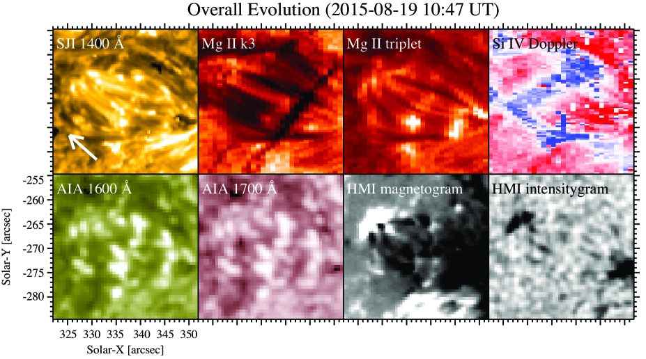
Figure 1: Composite of various observations to show the overall evolution of the target EFR. The corresponding movie provides the temporal evolution. From top left to bottom right, IRIS SJI 1400 Å, intensitygram at the Mg II k line core (k3), intensitygram at the Mg II triplet line, Dopplergram produced from the Si IV 1403 Å spectrum (blue, white, and red correspond to $-10$, $0$, and $+40\ {\rm km\ s}^{-1}$, respectively), SDO/AIA 1600 Å, 1700 Å, SDO/HMI magnetogram (black and white correspond to $-200$ and $200\ {\rm G}$, respectively), and intensitygram. The white arrow in the top left panel indicates the direction of the DC.

Figure 1 shows the overview of the target EFR in this study: see movie for the temporal evolution. In the center of the $30\arcsec\times 30\arcsec$ FOV, the HMI magnetogram shows that a number of tiny magnetic elements of positive and negative polarities (a few arcsec) emerge at the surface and separated each other in the northeast-southwest orientation. Eventually, the magnetic elements merge together to form pores at the edges of the EFR (see the HMI intensitygram: pore size $\sim 5\arcsec$).

At the same time, in the chromosphere, various brightening events are seen in different filtergrams (1400, 1600, and 1700 Å). They are located mostly in the central region with mixed magnetic polarities but also in the peripheral unipolar regions. The bright structures are seen to be larger in 1600 and 1700 Å images not only because of the large pixel sizes but also of the scattering effects (see, e.g., Rutten, 2016). Other filtergrams (e.g., 1330 and 2796 Å) exhibit similar brightening structures (not shown).

In the map of the Mg II k absorption line core (k3), an arch filament system (AFS) is clearly seen, which has an area of $\sim 30\arcsec\times 20\arcsec$ with a typical individual length of $\sim 20\arcsec$ and a width of $\sim 2\arcsec$. The Doppler velocity map obtained from the Si IV spectrum reveals a general trend that the EFR center (crests of the AFS) shows upflows and the peripheries (footpoints of the AFS) have downflows. These observational results are consistent with the H$\alpha$ observations reported by Bruzek (1967) and Bruzek (1969). The intensity of the Mg II triplet line between Mg II h and k is enhanced at the footpoints of the AFS.

3.2 Selection of Brightening Events

For surveying the variety of local heating events, we identified bright points (BPs) from the SOT Ca II H images. The intensity threshold for picking up such events is the 5$\sigma$ or higher above the mean of the AIA 1700 Å quiet-Sun values, which is suggested by Rutten et al. (2013).

Figure 2(a) shows a scatter diagram of 1700 Å intensity and Ca II H intensity. By fitting a straight line to this doubly logarithmic plot, we obtained the relation between the two data sets and found that the 5$\sigma+$mean criterion of the 1700 Å images, which is 4232.1 DN in the present data set, is equivalent to 1005.1 DN in the Ca images. We adopted this value for detecting the BPs in the Ca images and this criterion led to a total of 151 BPs from the sequential Ca data series in the period from 10:34 to 10:59 UT (25 frames).

Out of this 151 BPs, we found that 29 BPs were covered by the SOT SP scan. Figure 2(b) shows the distribution of the 29 BPs on the SOT SP circular polarization map (Stokes-V/I signal at 6301.43 Å), which represents the line-of-sight (LOS) component of the photospheric magnetic fields. Here, the BPs have a size of sub-arcsec to a few arcsec and are mostly seen in the magnetized regions.

We then checked the magnetic context of the 29 BPs using the degree of mixed polarity (Katsukawa & Tsuneta, 2005),

$$p_{\rm mix}=1-\left|\frac{|\Phi_{+}|-|\Phi_{-}|}{|\Phi_{+}|+|\Phi_{-}|}\right|,$$ (1)

where $\Phi_{\pm}$ is the total LOS flux of the positive ($+$) or negative ($-$) polarities within each BP patch. If $p_{\rm mix}=0$ the BP has either a positive or negative polarity (unipolar), while $p_{\rm mix}\neq 0$ indicates that the BP has both polarities within the Ca intensity contour (mixed-polarity). As a result, we found that there are seven mixed-polarity BPs and 22 unipolar BPs.

3.3 Spectral and Polarimetric Features

The 29 Ca BPs identified in Section 3.2 are classified into the following categories. The first group is the mixed-polarity events (seven BPs). They are distributed mostly in the center of the target EFR. The second and the third groups are the unipolar events in the limb-side, i.e., the south-western end of the EFR (five BPs) and in the DC-side, i.e., the north-eastern end (five BPs), respectively.

There are some remaining unipolar events, which are distributed in the EFR center (three BPs) and the plage regions outside the EFR (nine BPs). The general trends of these events are similar to those of the limb-side and DC-side unipolar events.

In this section, we introduce the spectral and polarimetric features of the mixed-polarity, limb-side unipolar, and DC-side unipolar events with showing the representative BPs.

3.3.1 Mixed-polarity Events

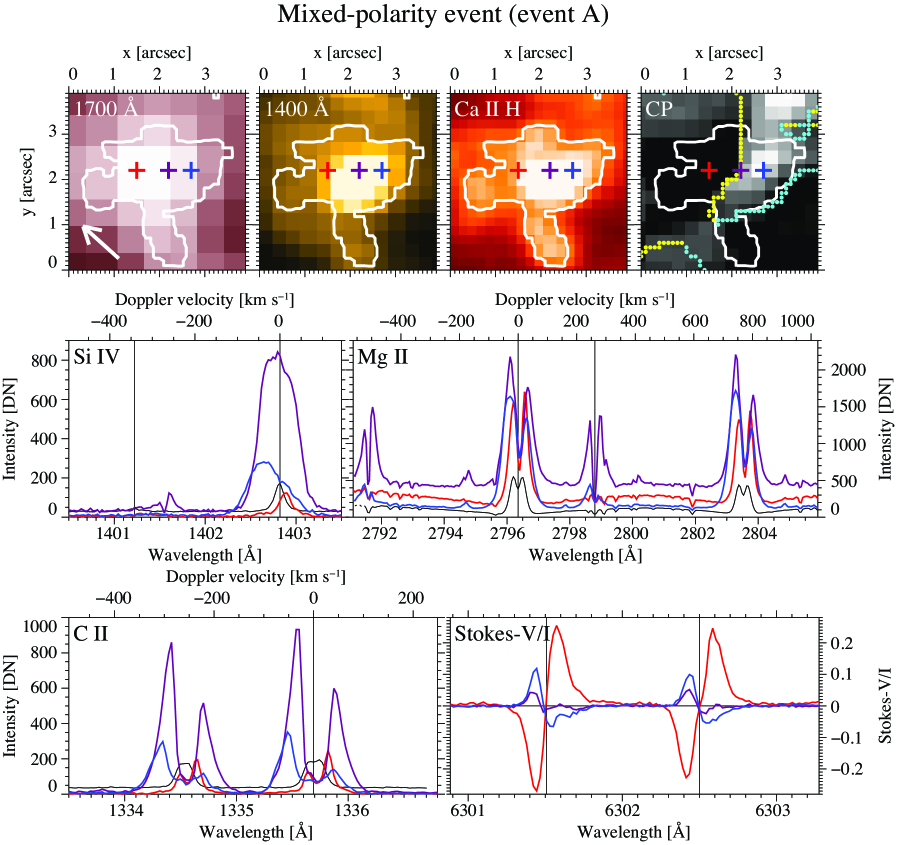
Figure 3: Spectral and polarimetric profiles of the sample mixed-polarity Ca BP (event A) located at $(X,Y)=(336\arcsec,-274\arcsec)$ in Figure 2(b). Four panels at the top are the filtergrams of AIA 1700 Å, IRIS SJI 1400 Å, SOT Ca II H, and the SOT SP circular polarization map. The white contour delineates the Ca BPs, while the white arrow in the 1700 Å image shows the direction of the DC. The dots in the circular polarization map indicate the locations of the PIL, where yellow and turquoise show that the magnetic fields have “dip” (i.e, bald-patch) and “top” structures, respectively (see text for details). Four bottom panels provide the IRIS spectra of Si IV, C II, and Mg II, and the SOT SP Stokes-V/I. The profiles of different colors (red, purple, blue) are sampled at three location indicated by the $+$ signs of corresponding colors in the top four images, while the black profiles are the averaged quiet-Sun levels obtained from the same data sets. In the Si IV and C II panels, the quiet-Sun profiles are multiplied by factors of 10. The vertical lines show the main lines and some blends, which are O IV 1401.2 Å, Si IV 1402.8 Å, Mg II k 2796.4 Å, Mg II triplet 2798.8 Å, C II 1335.7 Å, Fe I 6301.5 Å, and Fe I 6302.5 Å.

The mixed-polarity BPs are basically located in the central region of the EFR. A typical example of the mixed-polarity event is shown in Figure 3. This figure consists of three filtergrams and a circular polarization map of a BP located at $(X,Y)=(336\arcsec,-274\arcsec)$ in Figure 2(b) plus the IRIS spectra and SOT SP Stokes-V/I profiles for the three different locations within the BP.

Typically, in magnetized regions, Stokes-V/I has an antisymmetric profile with respect to the line center with two lobes of opposite signs in the red and blue wings. The three Stokes-V/I profiles in Figure 3 show a reversal of the sign, which indicates the transition of the LOS magnetic fields between positive (colored blue) and negative (red) polarities. At the central position of the BP located between the opposite polarities, the purple Stokes-V/I profile shows an asymmetric, irregular shape. Such shapes are often interpreted as a co-existence of closely neighboring two different magnetic components, e.g., positive and negative polarities, within a single pixel (Cheung et al., 2008), or as a complex stratification of magnetized atmosphere along the LOS direction.

One of the clearest characteristics of the mixed-polarity BPs is the strong enhancements of the line intensities and spectral widths. In Figure 3, the spectral lines have their maximum intensities at location indicated by the purple cross, i.e., at the BP center (see filtergrams and spectra). Among others, the peak intensity of Si IV spectrum is as much as 50 times higher than its quiet-Sun value. The purple profile at the BP center shows extended line wings of Doppler speeds of up to $\pm 100\ {\rm km\ s}^{-1}$. Morphologically, this BP has a size of about $3\arcsec\times 3\arcsec$ with a point-like bright core.

It is noteworthy here that the Doppler shifts of the IRIS spectra, especially of the transition-region lines (Si IV and C II), show a positional dependence. For example, the spectra indicated by red color, i.e., those of the DC side of the BP, have red-shifted profiles, indicating that the material at the transition-region temperature is flowing down. The Doppler velocity measured at the Si IV peak is about $20\ {\rm km\ s}^{-1}$. On the other hand, the blue-colored spectra, i.e., the limb-ward ones, are clearly blue-shifted, suggesting the upflow with an absolute velocity of $\sim 30\ {\rm km\ s}^{-1}$. Similar Doppler-shift dependency of the location (DC-ward or limb-ward) was recently reported by Vissers et al. (2015b).

The Mg II h and k spectra often exhibit double-peaked profiles with the so-called “self-absorption” cores. These central reversals are caused by the AFS (see Mg II k3 image of Figure 1), indicating that the Ca BPs are mostly covered by the thick and dense AFS material that exerts large opacity. Similarly, the C II spectra often show central reversals, too, while the Si IV do not in this data set.

The subordinate Mg II triplet line is sometimes seen in emission. In Figure 3, the triplet emission is exceptionally remarkable at the center of the BP (purple profile). According to Pereira et al. (2015), the triplet emission is rare and indicates a steep temperature increase above 1500 K in the lower chromosphere. These features are also reported by Vissers et al. (2015b) and Tian et al. (2016).

The circular polarization map in Figure 3 also shows the location of the polarity inversion lines (PILs), where the magnetic field has no radial component (i.e., $B_{z}=0$) and whether the magnetic structure at the PIL is “dip” or “bald patch”, in which the field lines have a concave-up configuration,

$$B_{z}=0\ {\rm and}\ \mbox{\boldmath$B$}\cdot\nabla B_{z}>0,$$ (2)

or “top”, in which the field lines are concave down,

$$B_{z}=0\ {\rm and}\ \mbox{\boldmath$B$}\cdot\nabla B_{z}<0$$ (3)

(Pariat et al., 2004; Watanabe et al., 2008). Since we have only a single-layer magnetogram, it would be better to explicitly describe the bald patch as

$$B_{z}=0\ {\rm and}\ B_{x}\frac{\partial B_{z}}{\partial x}+B_{y}\frac{\partial B_{z}}{\partial y}>0$$ (4)

and the counterpart as

$$B_{z}=0\ {\rm and}\ B_{x}\frac{\partial B_{z}}{\partial x}+B_{y}\frac{\partial B_{z}}{\partial y}<0.$$ (5)

Note that we here use the photospheric vector magnetic fields $(B_{x},B_{y},B_{z})$, which is transformed to the local Cartesian reference frame $(x,y,z)$ with $\hat{\mbox{\boldmath$z$}}$ being the local radial direction. It is clearly seen from the circular polarization map of Figure 3 that the PIL passes through the center of the Ca BP and that the magnetic fields have a bald-patch configuration (yellow dots). It is found that, in five mixed-polarity BPs out of the seven total events, the PIL is dominated by the bald patch: see Appendix A for PILs of the six remaining mixed-polarity BPs.

3.3.2 Unipolar Events: Limb-side

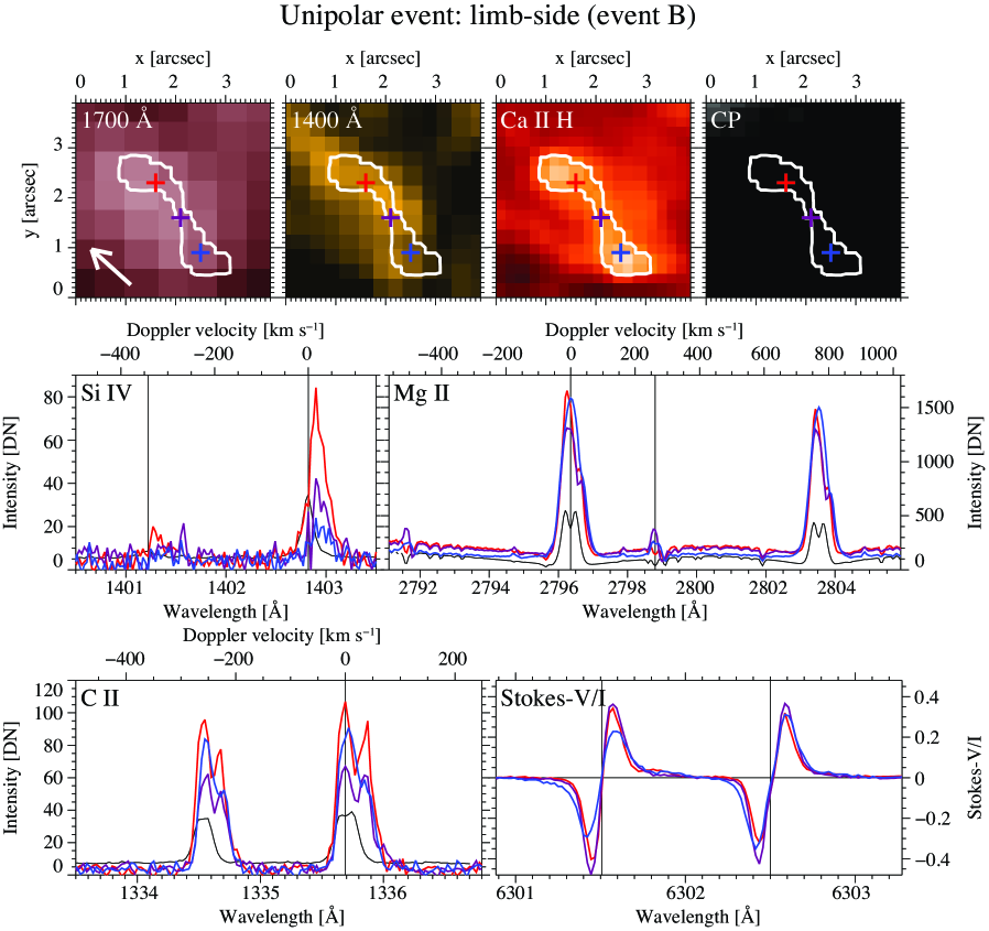
Figure 4: The same as Figure 3 but for the limb-side unipolar event (event B) at $(X,Y)=(350\arcsec,-270\arcsec)$ in Figure 2(b). The intensity scales of the top panels are identical to those of Figure 3. In the Si IV and C II panels, the quiet-Sun profiles are multiplied by factors of 2.

Figure 4 is a typical example of the unipolar BP in the limb-side of the target EFR. This BP is centered at $(X,Y)=(350\arcsec,-272\arcsec)$ in Figure 2(b). This location is one of the the south-western footpoints of the AFS (see Figure 1) and is surrounded by a large magnetic patch of the negative polarity. In the Stokes-V/I profiles, the unipolar nature of this BP is clearly reflected: they do not show a reversal or an irregular shape.

The line intensities are generally weaker than those of the mixed-polarity events. For example, the maximum intensities of the Si IV and C II lines in Figure 4 are at most five times of the quiet-Sun value, as opposed to much more than 10 times for the mixed-polarity events.

Another characteristic of the limb-side unipolar events is that the Si IV and C II spectra coherently show redshifts, i.e., downflows. In Figure 4, the Doppler velocity at the peak of the Si IV line reaches $30\ {\rm km\ s}^{-1}$.

It is also interesting that the Mg II lines do not show regular double-peaked profiles with central reversals but single-peaked (or top-flat) profiles. According to Carlsson et al. (2015), such single-peaked Mg II k profiles are found above the plage regions and imply the existence of hot and dense chromosphere of about 6500 K and a transition region at a high column mass. In fact, the single-peaked Mg II k profiles in this data set are seen mostly in the vicinity of or above the developing pores. Their Doppler shifts are not remarkable compared to those of the transition-region lines (Si IV and C II). It should also be noted that the Mg II triplet emission, which indicates the lower-chromospheric heating, are seen at some locations.

3.3.3 Unipolar Events: DC-side

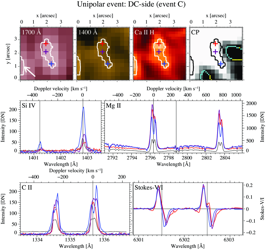
Figure 5: The same as Figure 3 but for the DC-side unipolar event (event C) at $(X,Y)=(328\arcsec,-266\arcsec)$ in Figure 2(b). The intensity scales of the top panels are identical to those of Figure 3. In the Si IV and C II panels, the quiet-Sun profiles are multiplied by factors of 4.

The second group of the unipolar BPs is located in the DC-side, i.e., the north-eastern end, of the target EFR. Figure 5 shows the sample event around $(X,Y)=(328\arcsec,-266\arcsec)$ in Figure 2(b).

This BP also exists at one footpoint of the AFS seen in the Mg II k3 images (Figure 1). The Stokes-V/I signals in Figure 5 show that this BP has a positive magnetic polarity with no irregular profiles. The line intensities are again weaker than those of the mixed-polarity events. Especially in the 1400 Å map, the intensity enhancement is much less marked.

The systematic redshifts are also seen in the Si IV and C II profiles. However, the redshift speeds of these events are generally smaller than those of the limb-side unipolar events. The maximum Doppler velocity of this BP (Figure 5) is $15.6\ {\rm km\ s}^{-1}$.

In Figure 5, the single-peaked Mg II k profiles (red and purple) are found near the pore, which is consistent with the limb-side unipolar events (Figure 4), while the blue Mg II k profile indicates that this location is probably covered by the AFS. Although not clear, Figure 5 shows an indication of a slight Mg II triplet emission.

3.3.4 Averaged Profiles

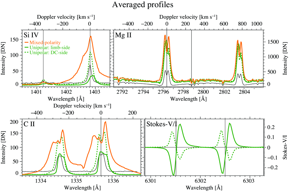
Figure 6: Averaged profiles of the Si IV, Mg II, C II, and Stokes-V/I for the seven mixed-polarity events (orange), five limb-side unipolar events (green solid), and five DC-side unipolar events (green dashed). The black curves and vertical lines are identical to those in Figure 3. In the Si IV and C II panels, the quiet-Sun profiles are multiplied by factors of 4.

Figure 6 compares the profiles of the Si IV, Mg II, C II, and Stokes-V/I averaged over the areas covered by the seven mixed-polarity BPs, five limb-side unipolar BPs, and five DC-side unipolar BPs.

The mixed-polarity events (orange) are characterized by their enhanced and broadened profiles, especially of the Si IV and C II lines. The peak intensities of the averaged Si IV and C II lines are about 9 times of the quiet-Sun levels, while their wings exceed $\pm 150\ {\rm km\ s}^{-1}$. The Mg II k has a double-peaked profile, which indicates that the mixed-polarity BPs are generally located below the fibrilar canopy of the AFS. The Mg II triplet emission is no more seen in this averaged profile because the triplet emission is rare and, if occurs, exists only in the cores of the BPs.

The clearest feature of the limb-side unipolar events (green solid), which shows a negative polarity in the Stokes-V/I profile, is the redshifts of the Si IV and C II spectra. These are caused by the systematic downflows at the footpoints of the AFS. The peak intensities of the Si IV and C II lines are darker, only twice and 4 times of their quiet-Sun values, respectively. Another obvious characteristic is the single-peaked shape of the Mg II k spectrum. Such a profile is created probably because these AFS footpoints are located above or very close to the developing pores. The Mg II triplet is seen in emission, indicating the heating of the lower chromosphere.

Compared to the limb-side events, the redshifts of the Si IV and C II lines of the DC-side, positive unipolar events (green dashed) are not very prominent, while the peak intensities of these lines show intermediate values between the mixed-polarity and the limb-side unipolar: six and eight times the quiet-Sun values. The Mg II k has an asymmetric profile with the central dip, probably caused by the mixture of the single-peaked profiles near the pores and the double-peaked ones under the AFS. Similar to the limb-side events, the Mg II triplet emission is seen.

3.4 Temporal Evolutions

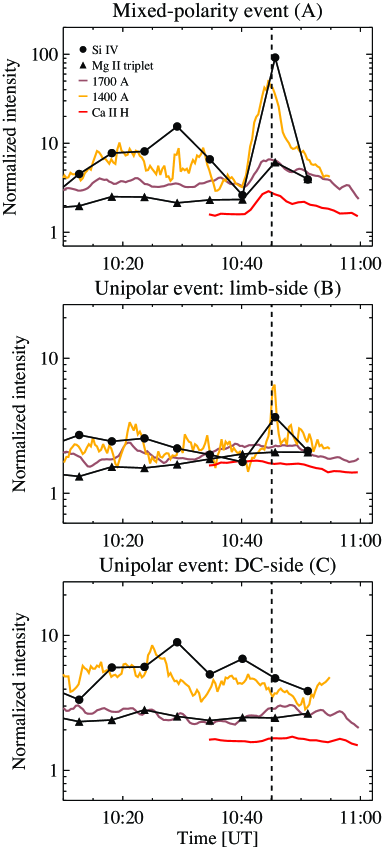
Figure 7: Temporal evolutions of the chromospheric and transition-region line intensities integrated over the $1\arcsec\times 1\arcsec$ box at the center of the BPs for the three representative events in Section 3.3. The plotted intensities of the Si IV and Mg II triplet lines are the intensities integrated over the spectral ranges of $\pm 0.5\ {\rm\AA}$ and $\pm 0.75\ {\rm\AA}$ from the line centers, respectively. All the intensities are normalized by the quiet-Sun values. Vertical dashed lines indicate the timing of the SOT SP scan.

Figure 7 plots the light curves of several chromospheric and transition-region lines for the three representative Ca BPs introduced in Section 3.3 (mixed-polarity, limb-side unipolar, and DC-side unipolar events). The light curves are obtained as time-varying intensities integrated over a $1\arcsec\times 1\arcsec$ box, centered at the middle of the BPs. In this figure, each light curve is normalized by its quiet-Sun value.

For the mixed-polarity event (Figure 7 top), the light curves show drastic enhancement around 10:45 UT with a duration of 10 to 15 minutes. They show similar evolution profiles with each other, a fast rise followed by an extended decay, which is highly reminiscent of the light curves of H$\alpha$ and soft X-rays recorded in the solar flares (e.g., Kane, 1974). The most significant enhancement is of the wavelength-integrated intensity of the Si IV line, which increases up to almost 100 times of its quiet-Sun level. Similar drastic Si IV enhancements of more than 10 times are seen for most of the mixed-polarity events.

Another feature to note for the mixed-polarity events is that the intensity enhancements are often repetitive at the same locations. For the mixed-polarity BP in Figure 7, the preceding event occurs about 20 minutes before the main one.

On the other hand, the light curves for both limb-side and DC-side unipolar events are generally less marked. The evolutions of typical events in Figure 7 (middle and bottom) are rather steady over time, and the normalized intensities become only a few times, at most 10 times, of the quiet-Sun levels. The most enhanced intensities are again of the Si IV spectra.

3.5 Statistical Trends

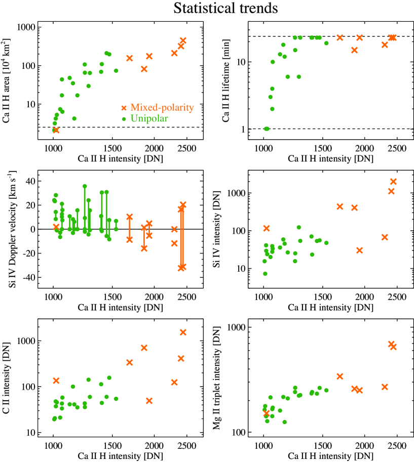
Figure 8: From top left to bottom right, scatter plots showing the maximum area and lifetime (or duration) measured in Ca II H, the maximum and minimum Doppler velocities measured from the Si IV spectra, the maximum intensities for the Si IV, C II, and Mg II triplet lines for all the mixed-polarity BPs (seven events: orange $\times$-marks) and unipolar BPs (22 events: green dots) as a function of Ca II H intensity.

The statistical trends for the analyzed 29 Ca BPs are shown in Figure 8. Here, the Ca intensities of both types of the BPs are clearly distinct. The mixed-polarity events are generally brighter than the unipolar ones with the critical value being $\sim 1600$ DN.

The maximum area of the Ca BPs is positively correlated with the intensity. Most of the mixed-polarity events have areas ranging from $0.8\times 10^{6}$ to $4.5\times 10^{6}\ {\rm km}^{2}$, which is equivalent to the radii of 500 to 1200 km if one assumes circular shapes. The unipolar BPs are $\lesssim 2\times 10^{6}\ {\rm km}^{2}$ in area, or of the radius of $\lesssim 800\ {\rm km}$. The Ca lifetime shows, although more than half of the measurements are limited by the cadence and the durations of the Ca observation by SOT, which are 1 minute and 25 minutes, respectively, a positive relation with the Ca intensity.

The plot for the maximum and minimum Doppler velocities, which is obtained by simply fitting a single Gaussian function to the Si IV profile, clearly shows the difference between the two groups. While the mixed-polarity events have a wider velocity range from $-32.4\ {\rm km\ s}^{-1}$ (blueshift) to $20.4\ {\rm km\ s}^{-1}$ (redshift), the unipolar ones are remarkably one-sided with a range of $-8.4$ to $35.7\ {\rm km\ s}^{-1}$, i.e., the downflows (redshifts) are dominated. Note that we here use the single-Gaussian fitting, which provides the Doppler velocity near the core of the spectrum and may be affected when the profile contains of more than two components.

The maximum intensities of the Si IV, C II, and Mg II triplet lines also show positive relations with the Ca II H intensity. However, the dynamic range for the Mg II triplet is less than one order of magnitudes, 120 to 690 DN, as opposed to the wider ranges of the Si IV and C II, 7.3 to 2000 DN and 19 to 1500 DN, respectively.

4 Summary

In this paper, we have investigated various local heating events in the EFRs using the co-observation data obtained by Hinode and IRIS, complemented by SDO. The main observational results of our study are summarized as follows.

The mixed-polarity events are seen in the central part of the EFR, which is characterized by enhanced and broadened chromospheric and transition-region spectra. In particular, the Si IV line brightens up significantly to 100 times of the quiet-Sun intensity. Sometimes the Si IV and C II spectra spread over the Doppler speeds of $\pm 150\ {\rm km\ s}^{-1}$. The Doppler velocities at the Si IV line center have a positional tendency that the redshifts of up to $20\ {\rm km\ s}^{-1}$ are seen in the DC side and the blueshifts of up to $30\ {\rm km\ s}^{-1}$ are seen in the limb side within the BP. The Mg II k spectra often show the central reversals, which is caused by the overlying AFS obscuration, while sometimes the Mg II triplet is seen in emission, indicating the lower chromospheric heating. These events are mostly found above the PILs with the bald-patch (i.e., U-shaped) magnetic configurations in the photosphere. They are larger in size, longer in lifetime. The light curves show flare-like evolutions with durations of 10 – 15 minutes and the brightenings recur with periods of about 20 minutes.

The unipolar events are mostly found in the peripheral regions of the EFR, i.e., the footpoints of the AFS. These events are weaker in intensities with the maximum Si IV intensity being at most 10 times of the quiet-Sun level. The Si IV spectra show systematic downflows with the maximum Doppler speed of $\sim 40\ {\rm km\ s}^{-1}$ at the line center. The redshift velocity is generally faster for the limb-side events than the DC-side events. If the BP is close to or above a pore, the Mg II k spectrum reveals a single-peaked profile with no absorption core, similar to the spectra found in the plage regions. The Mg II triplet is seen in emission occasionally. They are smaller in size, shorter in lifetime, and the evolution is steady.

5 Discussion

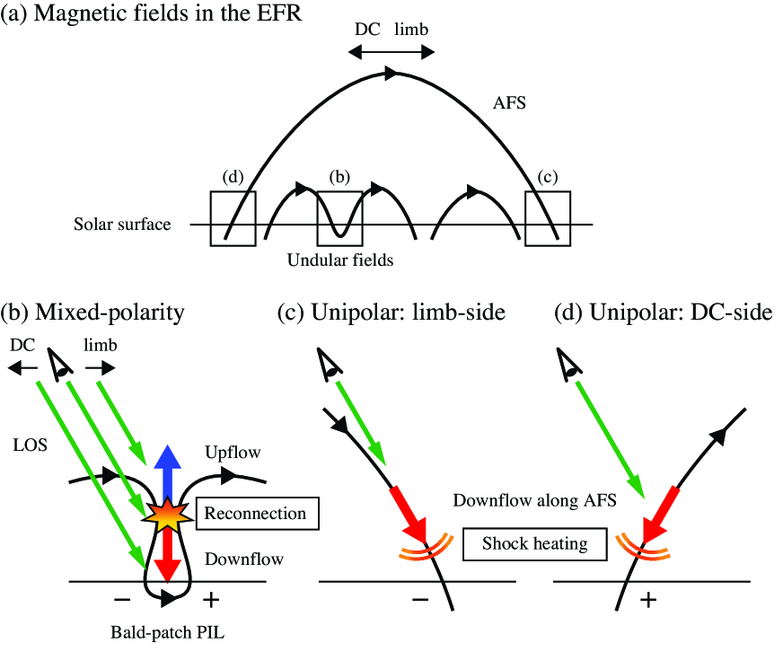
Figure 9: Schematic illustration summarizing the various local heating events in the EFRs. (a) Overview of the magnetic fields in the EFRs. Thick curve lines and a thin horizontal line indicate magnetic field lines and the solar surface. Three boxes show the regions corresponding to panels (b) to (d). (b) Mixed-polarity events, where the BP may represent the magnetic reconnection between the cancelling opposite magnetic polarities. The field line configuration is similar to Figure 12 of Georgoulis et al. (2002). Red and blue arrows indicate bi-directional jets, while the green arrows present the different LOSs. The $+$ and $-$ signs show the positive and negative polarities, respectively. (c and d) Limb-side and DC-side unipolar events, where the BP may be due to the shock heating caused by the fast downflows along the AFS. Orange curves represent the local heating.

The observational results summarized in Section 4 lend support to the physical picture illustrated in Figure 9. In EFRs, the magnetic fields appear at the photosphere as $\Omega$-shaped or undular field lines and evolve through episodes of merging and cancellations of fragmentary magnetic elements. The AFS is seen above, which may represent the ascending magnetic fields in the higher altitudes.

The observed mixed-polarity Ca BPs may indicate magnetic reconnection between the cancelling positive and negative polarities, as shown in Figure 9(b). Although we have no H$\alpha$ observation for our events, these BPs should be closely related to the classical Ellerman bombs (Ellerman, 1917). The striking consistencies may be found if one compares Figure 3 of this paper and Figure 4 of Vissers et al. (2015b), in which they show the IRIS and H$\alpha$ spectra of a textbook Ellerman bomb. Recently, Tian et al. (2016) and Grubecka et al. (2016) demonstrated that the Mg II h and k lines of Ellerman bombs show intense brightening in the wings and no significant enhancement in the core, similar to the H$\alpha$ profiles. The Mg II spectra in Figure 3 agree with this trend, which further supports that our events are likely Ellerman bombs.

Recent high-resolution observations indicate that the Ellerman bombs are the photospheric reconnection with flame-like structures (Watanabe et al., 2011; Vissers et al., 2013; Rutten et al., 2013). Such flames may not be resolved in our observations with a minimum pixel size of $0\farcs 22$ (Ca II H). Also, especially in 1700 Å, they may be blurred by scattering (Rutten, 2016).

The red and blueshifts observed in the mixed-polarity BPs can be interpreted as the bi-directional jets from the reconnection sites. The DC- and limb-ward dependence of the Doppler velocity may be due to the viewing angle. As the target EFR of this study is located away from the DC by $26^{\circ}$ – $27^{\circ}$, the slanted viewing angle may cause the sampling of upflows in the limb-side (or upper parts) and downflows in the DC-side (lower parts). Perhaps one might expect the siphon flow along the small $\Omega$-loop for explaining the red and blueshifts. However, the dominance of the bald-patch PILs for the mixed-polarity BPs favors the U-loop cancellation theory (Georgoulis et al., 2002; Pariat et al., 2004; Watanabe et al., 2008).

The unipolar BPs at the periphery of the EFR may be caused by the downflows (Figures 9(c) and (d)). Bruzek (1969) found the fast downdrafts of $\sim 50\ {\rm km\ s}^{-1}$ (in H$\alpha$) along the field lines of the AFS at both footpoints. Using magnetohydrodynamic (MHD) simulations, Shibata et al. (1989) modeled the EFRs and suggested that the bright plages near the AFS footpoints are caused by the shocks, which is produced by the fast downflows of 30 to $50\ {\rm km\ s}^{-1}$ along the AFS entering the high-density lower atmosphere. The above observations and simulations point to the possibility that the unipolar BPs in the present study are also due to the downflows.

If we simply assume a CHIANTI-based (i.e., coronal-equilibrium) Si IV formation temperature of $\log{T\,[{\rm K}]}=4.8$ – $4.9$ (De Pontieu et al., 2014; Peter et al., 2014), the local adiabatic sound speed is $\gtrsim 40\ {\rm km\ s}^{-1}$. However, it is more likely that the plasma at the AFS footpoints is denser and that the Si IV temperature is cooler than these values. Since Rutten (2016) suggests $15,000$ to $20,000\ {\rm K}$ for the Si IV temperature for the Ellerman bombs (the heating of low-chromospheric to mid-photospheric plasma), let us assume, say, $40,000\ {\rm K}$ as the temperature. Then, we obtain the sound speed of $\sim 30\ {\rm km\ s}^{-1}$. Therefore, there is a good chance that the downflows observed above the unipolar regions, whose Doppler velocity is up to $35.7\ {\rm km\ s}^{-1}$, are comparable to or exceed the local sound speed. Although we did not directly detect the shock fronts, considering that the Mg II lines are not strongly Doppler-shifted (Section 3.3.2) and that the typical sound speed in the photosphere is by far smaller, there may be shocks, or at least strong compressions and condensations of the material, which locally heat the atmosphere.

The differences of the observational characteristics between the limb-side and DC-side events, especially of the Doppler velocities, may be due to the viewing angle: compare Figures 9(c) and (d).

Perhaps this scenario has a relation with the transient supersonic downflows and associated heating events found above the sunspots by Kleint et al. (2014) and Tian et al. (2014). However, their downflows are by far faster, exceeding $200\ {\rm km\ s}^{-1}$, and probably are the material falling higher from the coronal heights such as coronal rain, as opposed to our steady, much slower downflows originated from the AFS.

The heating mechanisms suggested in this section explain the observations without inconsistencies and are, although not perfectly, supported by MHD simulations (e.g., Isobe et al., 2007; Tortosa-Andreu & Moreno-Insertis, 2009; Cheung et al., 2010; Shibata et al., 1989). However, especially for the heating in the unipolar regions, we cannot rule out other possibilities such as magnetic reconnection that we cannot resolve, or the component reconnection between the field lines of colliding magnetic patches of the same polarity (see, e.g., Figure 12c of Georgoulis et al. 2002). Therefore, it is of necessity to numerically model these mechanisms with taking into account the radiative transfer and examine the proposed scenarios.

Figure 2: (a) Scatter plot of the SOT Ca II H intensity versus the AIA 1700 Å intensity. Density contours in logarithmic scale are plotted for large density regions to avoid the plot saturation, while the logarithmic distributions for both parameters are shown at the right and top of the diagram. The vertical line indicates the $5\sigma+$mean level of the 1700 Å intensity and the horizontal line shows the equivalent value for the Ca II H intensity. (b) Distribution of the Ca BPs plotted on the SOT SP circular polarization map, identifying the 29 BPs analyzed in this study. Red contour indicates the Ca II H intensity level obtained in panel (a), while the red arrow at the bottom left shows the direction of the DC. A, B, and C label the three representative BPs introduced in Section 3.3.

Appendix A PILs of Mixed-polarity Events

Figure 10 summarizes the six remaining mixed-polarity events. Here, except for the two events (shown with red arrows), the PILs are dominated by the field lines with bald-patch configurations. Combined with the event introduced in Section 3.3.1, one can see that five out of seven total mixed-polarity BPs (71%) reveal bald-patch PILs. The event shown in the top middle panel of Figure 10 is separated in two patches with both “dip”-dominated and “top”-dominated PILs (red arrows), which may also support the importance of bald-patch PILs for the mixed-polarity events.

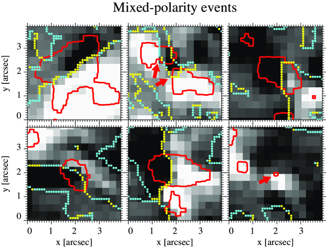
Figure 10: Six remaining mixed-polarity events located at (from top left to bottom right) $(X,Y)=(335\arcsec,-280\arcsec)$, $(328\arcsec,-274\arcsec)$, $(336\arcsec,-272\arcsec)$, $(336\arcsec,-265\arcsec)$, $(340\arcsec,-265\arcsec)$, and $(333\arcsec,-267\arcsec)$ in Figure 2(b). Each panel shows the SP circular polarization map (black-white), Ca II H contour (red) defining the Ca BPs, and locations of PILs (dots), where yellow and turquoise indicate that the magnetic fields have “dip” (i.e, bald-patch) and “top” structures, respectively. In the top-middle panel, a single event is separated into two patches at the moment of SOT SP scan.

References

- Asai et al. (2001) Asai, A., Ishii, T. T., & Kurokawa, H. 2001, ApJ, 555, L65
- Bruzek (1967) Bruzek, A. 1967, Sol. Phys., 2, 451
- Bruzek (1969) Bruzek, A. 1969, Sol. Phys., 8, 29
- Carlsson et al. (2015) Carlsson, M., Leenaarts, J., & De Pontieu, B. 2015, ApJ, 809, L30
- Cheung & Isobe (2014) Cheung, M. C. M., & Isobe, H. 2014, Living Reviews in Solar Physics, 11, 3
- Cheung et al. (2010) Cheung, M. C. M., Rempel, M., Title, A. M., & Schüssler, M. 2010, ApJ, 720, 233
- Cheung et al. (2008) Cheung, M. C. M., Schüssler, M., Tarbell, T. D., Title, A. M. 2008, ApJ, 687, 1373
- De Pontieu et al. (2014) De Pontieu, B., Title, A. M., Lemen, J. R., et al. 2014, Sol. Phys., 289, 2733
- Ellerman (1917) Ellerman, F. 1917, ApJ, 46, 298
- Georgoulis et al. (2002) Georgoulis, M. K., Rust, D. M., Bernasconi, P. N., & Schmieder, B. 2002, ApJ, 575, 506
- Grubecka et al. (2016) Grubecka, M., Schmieder, B., Berlicki, A., Heinzel, P., Dalmasse, K., & Mein, P. 2016, A&A, 593, A32
- Isobe et al. (2007) Isobe, H., Tripathi, D., & Archontis, V. 2007, ApJ, 657, 53
- Kane (1974) Kane, S. R. 1974, in IAU Symp. 57, Coronal Disturbances, ed. G. A. Newkirk (Cambridge: Cambridge Univ. Press), 105
- Katsukawa et al. (2007) Katsukawa, Y., Berger, T. E., Ichimoto, K., et al. 2007, Science, 318, 1594
- Katsukawa & Tsuneta (2005) Katsukawa, Y., & Tsuneta, S. 2005, ApJ, 621, 498
- Kitai (1983) Kitai, R. 1983, Sol. Phys., 87, 135
- Kleint et al. (2014) Kleint, L., Antolin, P., Tian, H., et al. 2014, ApJ, 789, L42
- Kosugi et al. (2007) Kosugi, T., Matsuzaki, K., Sakao, T., et al. 2007, Sol. Phys., 243, 3
- Lemen et al. (2012) Lemen, J. R., Title, A. M., Akin, D. J., et al. 2012, Sol. Phys., 275, 17
- Lites et al. (2013) Lites, B. W., Akin, D. L., Card, G., et al. 2013, Sol. Phys., 283, 579
- Lites et al. (2007) Lites, B., Casini, R., Garcia, J., & Socas-Navarro, H. 2007, Mem. Soc. Astron. Italiana, 78, 148
- Lites et al. (1995) Lites, B. W., Low, B. C., Martinez Pillet, V., et al. 1995, ApJ, 446, 877
- Pariat et al. (2004) Pariat, E., Aulanier, G., Schmieder, B., et al. 2004, ApJ, 614, 1099
- Pereira et al. (2015) Pereira, T. M. D., Carlsson, M., De Pontieu, B., & Hansteen, V. 2015, ApJ, 806, 14
- Pesnell et al. (2012) Pesnell, W. D., Thompson, B. J., & Chamberlin, P. C. 2012, Sol. Phys., 275, 3
- Peter et al. (2014) Peter, H., Tian, H., Curdt, W., et al. 2014, Science, 346, 1255726
- Roy (1973) Roy, J. R. 1973, Sol. Phys., 28, 95
- Rutten (2016) Rutten, R. J. 2016, A&A, 590, A124
- Rutten et al. (2013) Rutten, R. J., Vissers, G. J. M., Rouppe van der Voort, L. H. M., Sütterlin, P., & Vitas, N. 2013, Journal of Physics Conference Series, 440, 012007
- Scherrer et al. (2012) Scherrer, P. H., Schou, J., Bush, R. I., et al. 2012, Sol. Phys., 275, 207
- Schmieder et al. (2014) Schmieder, B., Archontis, V., & Pariat, E. 2014, Space Sci. Rev., 186, 227
- Schou et al. (2012) Schou, J., Scherrer, P. H., Bush, R. I., et al. 2012, Sol. Phys., 275, 229
- Shibata et al. (1992) Shibata, K., Ishido, Y., Acton, L. W., et al. 1992, PASJ, 44, L173
- Shibata & Magara (2011) Shibata, K., & Magara, T. 2011, Living Reviews in Solar Physics, 8, 6
- Shibata et al. (1989) Shibata, K., Tajima, T., Steinolfson, R. S., & Matsumoto, R. 1989, ApJ, 345, 584
- Spruit & Scharmer (2006) Spruit, H. C., & Scharmer, G. B. 2006, A&A, 447, 343
- Strous et al. (1996) Strous, L. H., Scharmer, G., Tarbell, T. D., Title, A. M., & Zwaan, C. 1996, A&A, 306, 947
- Tian et al. (2014) Tian, H., Kleint, L., Peter, H., et al. 2014, ApJ, 790, L29
- Tian et al. (2016) Tian, H., Xu, Z., He, J., & Madsen, C. 2016, ApJ, 824, 96
- Toriumi et al. (2015b) Toriumi, S., Cheung, M. C. M., & Katsukawa, Y. 2015b, ApJ, 811, 138
- Toriumi et al. (2014) Toriumi, S., Hayashi, K., & Yokoyama, T. 2014, ApJ, 794, 19
- Toriumi et al. (2015a) Toriumi, S., Katsukawa, Y., & Cheung, M. C. M. 2015a, ApJ, 811, 137
- Tortosa-Andreu & Moreno-Insertis (2009) Tortosa-Andreu, A., & Moreno-Insertis, F. 2009, A&A, 507, 949
- Tsuneta et al. (2008) Tsuneta, S., Ichimoto, K., Katsukawa, Y., et al. 2008, Sol. Phys., 249, 167
- Vissers et al. (2015a) Vissers, G. J. M., Rouppe van der Voort, L. H. M., & Carlsson, M. 2015a, ApJ, 811, L33
- Vissers et al. (2013) Vissers, G. J. M., Rouppe van der Voort, L. H. M., & Rutten, R. J. 2013, ApJ, 774, 32
- Vissers et al. (2015b) Vissers, G. J. M., Rouppe van der Voort, L. H. M., Rutten, R. J., Carlsson, M., & De Pontieu, B. 2015b, ApJ, 812, 11
- Watanabe et al. (2008) Watanabe, H., Kitai, R., Okamoto, K., et al. 2008, ApJ, 684, 736
- Watanabe et al. (2011) Watanabe, H., Vissers, G., Kitai, R., Rouppe van der Voort, L., & Rutten, R. J. 2011, ApJ, 736, 71
- Zwaan (1985) Zwaan, C. 1985, Sol. Phys., 100, 397