Constraints on the dynamical evolution of the galaxy group M81

Abstract

According to the standard model of cosmology, galaxies are embedded in dark matter halos which are made of particles beyond the standard model of particle physics, thus extending the mass and the size of the visible baryonic matter by typically two orders of magnitude. The observed gas distribution throughout the nearby M81 group of galaxies shows evidence for past significant galaxy–galaxy interactions but without a merger having occurred. This group is here studied for possible dynamical solutions within the dark-matter standard model. In order to cover a comprehensive set of initial conditions, the inner three core members M81, M82 and NGC 3077 are treated as a three-body model based on Navarro-Frenk-White profiles. The possible orbits of these galaxies are examined statistically taking into account dynamical friction. Long living, non-merging initial constellations which allow multiple galaxy–galaxy encounters comprise unbound galaxies only, which are arriving from a far distance and happen to simultaneously encounter each other within the recent 500 Myr. Our results are derived by the employment of two separate and independent statistical methods, namely a Markov chain Monte Carlo method and the genetic algorithm using the SAP system environment. The conclusions reached are confirmed by high-resolution simulations of live self-consistent systems (N-body calculations). Given the observed positions of the three galaxies the solutions found comprise predictions for their proper motions.

1 Introduction

The law of gravitation by Newton and its reformulation as a geometrical space-time distortion through matter by Einstein has been empirically derived within the Solar system. It is commonly extrapolated, by orders of magnitude, to the very strong and very weak curvature regimes (Koyama, 2016). However, in the very weak curvature regime the extrapolation fails to account for the observations, such as the flat shape of the rotation curves of galaxies. One attempt at solving this extrapolation is to hypothesize that the observed deficit comes about due to the presence of particle dark matter, therewith proposing an extension of the standard model of particle physics. In the standard dark-energy plus cold-dark-matter model of cosmology (LCDM) the new particles must only interact gravitationally and at most weakly with each other and with the variety of known particles of the standard model of particle physics.

The question whether the existence of dark matter halos can be inferred observationally has a long history. While the approximately flat rotation curves to large radii observed in disk galaxies unambiguously imply either particle dark matter halos or non-Newtonian gravitation (Famaey & McGaugh, 2012), the potentials around elliptical galaxies are much less constrained because of the lack of observable tracers and because velocity anisotropies confuse the dynamical evidence (e.g. Samurović & Danziger 2005, Samurović 2006, Samurović & Ćirković 2008, Samurović 2014 and Richtler et al. 2011).

One important testable implication of the particle dark matter halos is that they imply significant dynamical friction when a galaxy encounters another galaxy (Kroupa, 2015). Indeed, “Interacting galaxies are well-understood in terms of the effects of gravity on stars and dark matter” (Barnes, 1998), and interacting major galaxies merge within about 1-1.5 Gyr after infall (Privon et al., 2013). This is the sole origin of the hierarchical, merger-driven formation of structure in the LCDM model, which is popularly assumed to be the main physical process driving the formation and evolution of the galaxy population observed at the present cosmological epoch. Thus, if observed galactic systems show either evidence for dynamical friction or absence of this important process then this would test the presence of dark matter halos (Kroupa, 2015).

Located about 3.6 Mpc from the Local Group of galaxies, the M81 group of galaxies is the closest similar constellation of galaxies. It therefore offers opportunities for the investigation of the dynamical behavior of such loose but typical groups of galaxies, based on thorough available observational data. Thus, if information exists which constrains the past encounters between group members then the process of dynamical friction can be tested for. For example, the Local Group of galaxies is constrained by the two major galaxies not allowed to have merged, such that Andromeda and the Milky Way never had a close encounter in the past if the LCDM is valid (Zhao et al., 2013).

The M81 group of galaxies is comprised of a major Milky-Way type galaxy (M81, baryonic mass $M_{\rm M81}$ $\approx$ 3 $\cdot~{}10^{10}M_{\odot}$) and four companion galaxies, two of which are themselves dwarf but nevertheless substantial star-forming disk galaxies (M82, $M_{\rm M82}$ $\approx$ 1 $\cdot~{}10^{10}M_{\odot}$ and NGC 3077, $M_{\rm N3077}$ $\approx$ 2 $\cdot~{}10^{9}M_{\odot}$). The interesting observational finding is that these galaxies are enshrouded by HI-emitting gas spanning the dimensions of the inner group which is about 50-100 kpc. This requires the galaxy pairs M81/M82 and M81/NGC 3077 to have interacted closely at least once, in order to strip the outer gaseous disks and rearrange the matter in the long tidal features (Cottrell 1977, Gottesman & Weliachev 1977, van der Hulst 1979, Yun et al. 1993 and Yun et al. 1994). This constrains the distribution of dark matter in the group by the process of dynamical friction, because the time span between the encounters and the merging due to dynamical friction is constrained to be at least about a crossing time, i.e. about 0.5–1 Gyr (for a typical velocity of $200\,$km/s and over a spatial range of 50–100 kpc).

The M81 group must have assembled through the infall of the individual galaxies according to the merger tree which is a necessary part of the hierarchical structure formation in the LCDM model. The currently observed configuration of the M81 group constrains the pre-infall initial conditions since for example tightly bound initial conditions are most likely ruled out given that the M81 group has not merged yet to an early-type galaxy. Full-scale simulations of live self-gravitating disk galaxies, each with their inter-stellar media are too prohibitive, given that only four dimensional observational information is available in six-dimensional phase space, to allow a wide scan of parameters to seek those pre-infall configurations which lead to the presently observed group structure. Therefore, as a first step simplified but very rapid simulations are performed here taking into account the essential physical process, namely dynamical friction on the putative dark matter halos. For this purpose the three-particle integration is combined in a novel approach with the genetic algorithm and the Markov chain Monte Carlo method to yield robust estimates of the allowed pre-infall configurations.

Thus, as a first step, we perform numerical simulations of the possible orbits of the three core members M81, M82 and NGC 3077, treated as a three-body problem with rigid Navarro-Frenk-White profiles (NFW, Navarro et al. 1995) for the DM halos. Based on the knowledge of today’s plane of sky (POS) coordinates, the distances and the radial velocities, as well as the knowledge about the North Tidal Bridge (NTB) and South Tidal Bridge (STB) obtained by radio astronomical observations, two different methods (Markov chain Monte Carlo (MCMC) and genetic algorithm(GA)) are utilized for the delivery of statistical populations for the unknown, or just roughly known physical entities under the constraint that known conditions be fulfilled. For a comprehensive statistical evaluation, the simplified three-body model serves as a first basis since numerical N-body simulations wouldn’t allow a comprehensive scan of initial parameters within an appropriate project time. By then comparing individual solutions with high-resolution simulations of live self-consistent systems the results of these estimates are verified.

In Section 2 we briefly discuss the impact of dark matter (DM) halos on the orbits of bodies upon intruding their interior and present the model for the Coulomb logarithm examined in this publication. Section 3 presents facts about the M81 group important for our investigations, and our approach how to achieve meaningful statistical results concerning their dynamical behaviour. Sections 4 and 5 deal with the details of our application of the mentioned statistical methods, MCMC and GA, to the inner M81 group and the results obtained there, followed by a general discussion comparing those methods (Section 6). In Section 7 we present the results of individual N-body calculations compared to the orbits of our three-body calculations, randomly extracted from the statistical population. Finally, in Section 8 we discuss the results obtained. For easy reading, Appendix B provides a list of acronyms used in this publication.

2 Dark Matter Halos and Dynamical Friction

Exploring the dynamics of bodies travelling along paths in the interior of DM halos implies that the effects of dynamical friction have to be taken into account in an appropriate manner (Chandrasekhar, 1942). For isotropic distribution functions the decelaration of an intruding body due to dynamical friction is described by Chandrasekhar’s formula (Chandrasekhar, 1943), which reads for a Maxwellian velocity distribution with dispersion $\sigma$ (for details see Binney & Tremaine (2008), chap. 8.1):

$$\frac{d\vec{\textbf{v}}_{M}}{dt}=-\frac{4{\pi}G^{2}M{\rho}}{{\textnormal{v}_{M}}^{3}}\ \textnormal{ln}{\Lambda}\left[\textnormal{erf}(X)-\frac{2X}{\sqrt{{\pi}}}\textnormal{e}^{-X^{2}}\right]\vec{\textbf{v}}_{M}\ ,$$ (1)

with X = v_M/($\sqrt{2}\sigma$). The intruder of mass M and relative velocity $\vec{\textbf{v}}_{M}$ is decelareted by $d\vec{\textbf{v}}_{M}$/dt in the background density $\rho$ of the DM halo.

Simulating galaxy-galaxy encounters Petsch & Theis (2008) showed that a modified model for the Coulomb logarithm ln$\Lambda$, originally proposed by Jiang et al. (2008), describes the effects of dynamical friction in a realistic manner. This mass- and distance-dependent model reads:

$$\textnormal{ln}\Lambda=\textnormal{ln}\left[1+\frac{M_{halo}(r)}{M}\right]\ ,$$ (2)

where $M_{halo}(r)$ is the mass of the host dark matter halo within radial distance $r$.

Chandrasekhar’s formula only gives an estimate at hand. However, high-resolution simulations of live self-consistent systems presented in Section 7 confirm our approach of employing this semi-analytical formula in our three-body calculations.

3 The inner Group

As already indicated, the three core members M81, M82 and NGC 3077 are treated as a three-body system, based on rigid NFW-profiles for the DM halos. In our notation the indices 1, 2 and 3 represent M81, M82 and NGC 3077, respectively. M81 appears to be the most massive object accompanied by M82 and NGC 3077.

3.1 Observational Data

The observational data for the plane-of-sky (POS) coordinates and the radial velocities are taken from the NASA/IPAC Extragalactic Database (NED), query submitted on 8 Feb 2014, and are presented in Table 1. The distances, however, are only roughly known: even for M81 an uncertainty of about 10% due to the variation of recent results published over the last decade can be extracted from NED. In our context we are interested in the relative distances of the three core members related to the M81 frame at present, rather than absolute distances. Therefore we take the average value for M81 as granted and cater for the mentioned uncertainty by means of appropriate ranges for the distances of the companions M82 and NGC 3077, as shown in Table 1. As a final remark regarding the phase space, the POS velocity components are not known at all.

Apart from optical observations, radio astronomical data are at our disposal. M81, M82 and NGC 3077 are known to be embedded in a large cloud of atomic hydrogen as observations of the 21cm HI emission line have shown (Appleton et al., 1981). Cottrell (1977) and Gottesman & Weliachev (1977) identified the NTB connecting M81 and M82, as van der Hulst (1979) did for the STB between M81 and NGC 3077. The results of those observations were confirmed by Yun et al. (1993) and Yun et al. (1994) by investigating the inner M81 group with the Very Large Array Telescope. Since then, the fact that both companions must have experienced close encounters with M81 in the recent cosmological past has been commonly agreed to be an established feature of the inner group. A review of the entire situation is presented by Yun (1999).

Object	RA	DEC	Heliocentric	Distance	$L_{\textnormal{v}}$	Baryonic Mass	DM Halo Mass
	(EquJ2000)	(EquJ2000)	Velocity		(visual)	($M_{\odot}$)	($M_{\odot}$)
M81	09h55m33.2s	+69d03m55s	-34 km/s	$3.63\ Mpc$	2.04 $\cdot~{}10^{10}$	3.06 $\cdot~{}10^{10}$	1.17 $\cdot~{}10^{12}$
M82	09h55m52.7s	+69d40m46s	203 km/s	$(3.53\pm 0.6)\ Mpc$	8.70 $\cdot~{}10^{9}$	1.305 $\cdot~{}10^{10}$	5.54 $\cdot~{}10^{11}$
NGC 3077	10h03m19.1s	+68d44m02s	14 km/s	$(3.83\pm 0.6)\ Mpc$	1.95 $\cdot~{}10^{9}$	2.925 $\cdot~{}10^{9}$	2.43 $\cdot~{}10^{11}$

Table 1: Observational and derived data for the inner M81 group members.

3.2 Previous Results

Thomasson & Donner (1993) simulated the tidal interaction between M81 and NGC 3077, reproducing the STB and the spiral structure of M81. The orbit generating the best fit shows a pericentre passage with a distance of 22 kpc about 400 Myr ago (i.e. at time $-400\,$Myr).

Yun (1999) additionally considered the tidal interaction between M81 and M82, too, reproducing the NTB as well as the STB. The pericentre passages occur at -220 Myr with a separation of 25 kpc and at -280 Myr with a separation of 16 kpc for M82 and NGC 3077, respectively. (A GIF-movie is still available at http://www.aoc.nrao.edu/$\sim$myun/movie.gif).

Full N-body simulations by Thomson et al. (1999) for the three core members did not yield satisfactory results because the galaxies merge. Indeed, due to the effect of dynamical friction within the DM halos, the solutions found by Yun (1999) and Thomson et al. (1999) would result in merged galaxies. Obviously, this begs the question how likely it is to catch the M81 system, which is also the next and nearest Local Group equivalent, just in this special evolution phase after the close encounters between its inner three members and before any one of them has merged. Further investigations of the behaviour of the inner M81 group have not been published since Yun (1999) and Thomson et al. (1999).

3.3 DM halo masses

Following Behroozi et al. (2013) we derived the baryonic and DM Halo masses from the bolometric luminosities, as extracted fom NED (query submitted on 3 Nov 2015). The results are shown in Table 1.

The masses of the DM halos listed in Table 1 may appear very high compared to the baryonic masses. However, following fig. 7 and 8 in Behroozi et al. (2013) DM-to-baryonic mass ratios of the order of 100:1 are expected for the baryonic masses listed in Table 1. The lowest ratio is about 40:1 at a DM halo mass of $10^{12}\,M_{\odot}$, as can be seen for M81.

This is in line with Binney & Tremaine (2008) (p. 18, table 1.2), who quote for the M81 comparable Milky Way a baryonic mass of $5\cdot 10^{10}\,M_{\odot}$, and a DM halo mass of $2\cdot 10^{12}\,M_{\odot}$.

3.4 The Model

The DM halo of either galaxy is treated as a rigid halo with a density profile according to Navarro et al. (1995) (NFW-profile), truncated at the the radius $R_{200}$:

$$\rho(r)=\frac{\rho_{0}}{r/R_{s}\left(1+r/R_{s}\right)^{2}}\ ,$$ (3)

with $R_{s}=R_{200}/c$, $R_{200}$ denoting the radius yielding an average density of the halo of 200 times the cosmological critical density

$$\rho_{crit}=\frac{3H^{2}}{8\pi G}\ ,$$ (4)

and the concentration parameter $c$

$$\log_{10}c=1.02-0.109\left(\log_{10}\frac{M_{\mathrm{vir}}}{10^{12}M_{\odot}}\right)\$$ (5)

(see Macciò et al. (2007)). The parameters for the three NFW-profiles are presented in Table 2.

Object	$R_{200}(kpc)$	$\rho_{0}$ ($M_{\odot}/pc^{3}$)	$c$
M81	210.4	7.210 $\cdot~{}10^{-3}$	10.29
M82	164.0	8.810 $\cdot~{}10^{-3}$	11.17
NGC 3077	124.6	1.100 $\cdot~{}10^{-2}$	12.22

Table 2: NFW profile parameters for the inner M81 group members.

As explained in Section 2 in case of overlapping DM halos, not only the gravitational force derived from the NFW profiles but also the effect of dynamical dissipation has to be taken into account. As an example, the Coulomb logarithm (Eq. 2) to be incorporated in Eq. 1 is displayed in Figure 1 for either companion M82 and NGC 3077 penetrating M81’s DM halo.

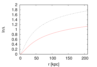
Figure 1: The Coulomb logarithm ln$\Lambda$ for M82 (lower curve) and NGC 3077 (upper curve) penetrating the DM halo of M81, shown as a function of the distance from the DM halo centre of M81.

In the M81 reference frame, at present, with $x1=y1=z1=0$ and $v_{1_{x}}=v_{1_{y}}=v_{1_{z}}=0$, our three-body problem is described by the POS coordinates and radial velocities of the two companions M82 and NGC 3077 relative to M81, deducted from Table 1, their unknown POS velocity components, and their roughly known relative distances also derived from Table 1. Table 3 shows the full set of open parameters.

The details regarding the numerical solution for the calculation of the forces between the galaxies, as well as the details concerning the numerical solution of the dynamical equations thereafter are presented in Appendix C. Figure 2 shows the forces between the galaxies due to gravity and dynamical friction, dependent on the relative velocities.

$P_{1}$	$P_{2}$	$P_{3}$	$P_{4}$	$P_{5}$	$P_{6}$
$v_{2_{x}}$	$v_{2_{y}}$	$z_{2}$	$v_{3_{x}}$	$v_{3_{y}}$	$z_{3}$

Table 3: Open parameters for the inner M81 group.

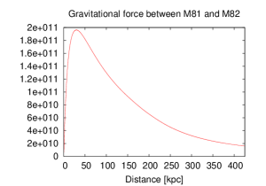
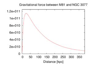
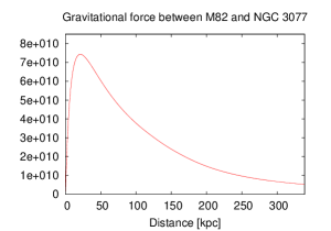
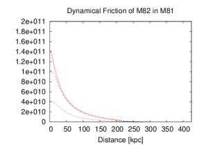
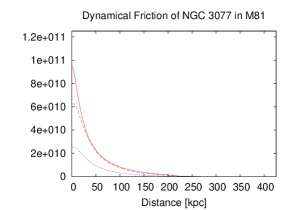
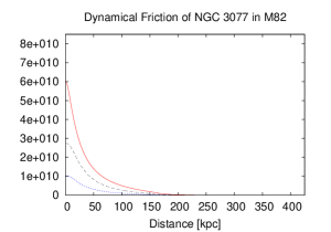
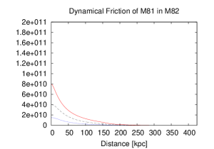
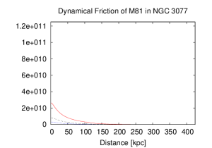
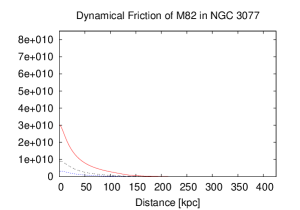
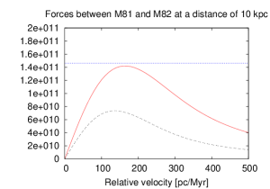
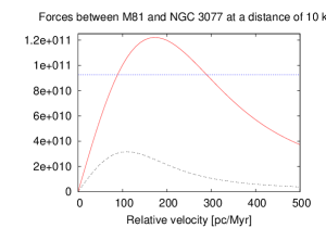
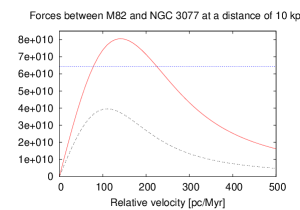
Figure 2: The variety of forces between the galaxies presented in galactic units ($M_{\odot}$, pc, Myr). First row: The gravitational forces between M81 and M82 (left), M81 and NGC 3077 (centre) and M82 and NGC 3077 (right). The distances between the centres of the galaxies are extended by 50 kpc beyond the separation distance of the DM halos, thus visualizing the continous transition to Newton’s law of gravitation for point masses upon separation. Second row: Forces, caused by dynamical friction, on M82 moving in the DM halo of M81 (left), NGC 3077 in M81 (centre) and NGC 3077 in M82 (right), for relative velocities of 100 pc/Myr (top curves), 300 pc/Myr (middle curves) and 500 pc/Myr (bottom curves). Third row: Same as second row, but vice versa. Fourth row: Forces due to gravitation (constant values) and dynamical friction at a separation distance of 10 kpc between the centres of the DM halos, shown in dependence on the relative velocity. Left: M82 in M81 (top curve) and M81 in M82 (bottom curve). Centre: NGC 3077 in M81 (top curve) and M81 in NGC 3077 (bottom curve). Right: NGC 3077 in M82 (top curve) and M82 in NGC 3077 (bottom curve).

3.5 Approach

At first, calculating three-body orbits backwards up to $-7$ Gyr, statistical populations for the open parameters (Table 3) are generated by means of the methods of Sections 4 (MCMC) and 5 (GA). Following the results of the previous publications mentioned in Section 3.2 we added, additionally to the known initial conditions at present, the rather general condition (later referred to as COND) that both companions M82 and NGC 3077 encountered M81 within the recent 500 Myr at a pericentre distance below 30 kpc.

Each three-body orbit of those populations is fully determined by all the known and open parameters provided by either MCMC or GA. Starting at time $-7$ Gyr and calculating the corresponding three-body orbits forward in time up to $+7$ Gyr, the behaviour of the inner group is investigated with respect to the question of possibly ocurring mergers in the future.

4 Statistical Methods I: Markov Chain Monte Carlo

We follow a methodology proposed by Goodman & Weare (2010) employing an affine-invariant ensemble sampler for the Markov chain Monte Carlo method (MCMC). A solid instruction ”how to go about implementing this algorithm” can be found in Foreman-Mackey et al. (2013), who also provide an online link to a Python implementation. However, we decided to realize this algorithm on our own utilizing the ABAP development workbench (see Appendix A). The basics of applying this formalism to our situation are outlined in Appendix D.

4.1 Definition of the Posterior Probability Density

First of all, concerning the open parameters, we need to account for the distance ranges specified in Table 1 as well as the fact that realistic velocities should be considered. This is ensured by an appropriate definition of the prior distribution $p(\vec{X})$.

Regarding the distance ranges for M82 and NGC 3077 we define ($i=2,3$)

$$p_{z}(\vec{X})_{i}\propto\left\{\begin{array}[]{ll}\exp\left({-{\displaystyle\frac{\left({z_{i}}-{z_{min}}\right)^{2}}{2\cdot{z_{0}}^{2}}}}\right),&z_{i}<z_{min}\ ,\\ \exp\left({-{\displaystyle\frac{\left({z_{i}}-{z_{max}}\right)^{2}}{2\cdot{z_{0}}^{2}}}}\right),&z_{i}>z_{max}\ ,\\ 1,&\textrm{otherwise}\ ,\\ \end{array}\right.$$ (6)

with the appropriate values for $z_{min}$ and $z_{max}$ for either companion derived from Table 1, and a value of 100 kpc for $z_{0}$. To account for realistic velocities $v_{i}=\ \mid\vec{v}_{i}\mid$ (about $\leq$ 500 km/s) in the centre-of-mass frame we implemented ($i=2,3$)

$$p_{v}(\vec{X})_{i}\propto\left\{\begin{array}[]{ll}1,&v_{i}\leq v_{max}\ ,\\ \exp\left({-{\displaystyle\frac{\left({v_{i}}-{v_{max}}\right)^{2}}{2\cdot{v_{0}}^{2}}}}\right),&v_{i}>v_{max}\ ,\end{array}\right.$$ (7)

with $v_{max}$ = 400 pc/Myr and $v_{0}$ = 100 pc/Myr. All together our prior distribution is given by

$$p(\vec{X})\ \propto\ \prod_{i=2}^{3}\ p_{z}(\vec{X})_{i}\ \cdot\ p_{v}(\vec{X})_{i}\ .$$ (8)

Exploiting the minimal distances $d_{12}$ and $d_{13}$ within the recent 500 Myr between M81/M82 and M81/NGC 3077, respectively, the condition COND specified in Section 3.5 is incorporated by the following contribution to the likelihood function ($i=2,3$):

$$P_{C}(\vec{X}\mid D)_{i}\propto\left\{\begin{array}[]{ll}1,&d_{1i}\leq d_{per}\ ,\\ \exp\left({-{\displaystyle\frac{\left({d_{1i}}-{d_{per}}\right)^{2}}{2\cdot{d_{0}}^{2}}}}\right),&d_{1i}>d_{per}\ ,\end{array}\right.$$ (9)

with $d_{per}$ = 25 kpc and ${d_{0}}$ = 5 kpc. Denoting the initial velocities at $-7$ Gyr (prior to the encounters) in the centre-of-mass frame by $u_{i}=\mid\vec{u}_{i}\mid$, we generate realistic values for those by

$$P_{u}(\vec{X}\mid D)_{i}\propto\left\{\begin{array}[]{ll}1,&u_{i}\leq v_{max}\ ,\\ \exp\left({-{\displaystyle\frac{\left({u_{i}}-{v_{max}}\right)^{2}}{2\cdot{v_{0}}^{2}}}}\right),&u_{i}>v_{max}\ ,\end{array}\right.$$ (10)

taking the same values for $v_{max}$ and $v_{0}$ as in Eq. 7. Assembling both aspects we arrive at the likelihood function

$$P(\vec{X}\mid D)\ \propto\ \prod_{i=2}^{3}\ P_{C}(\vec{X}\mid D)_{i}\ \cdot\ P_{u}(\vec{X}\mid D)_{i}\ .$$ (11)

4.2 The First Ensemble

Generating random numbers $n\in\{0,...,1000\}$ separately for each walker and open parameter, the first ensembles are created according to ($i\in\{1,...,6\}$)

$$P_{i}=(P_{i})_{min}+n\cdot\left[(P_{i})_{max}-(P_{i})_{min}\right]/1000\ .$$

The minimum and maximum values for the distances are derived from Table 1, and for the POS velocity components chosen to be $\pm$ 500 pc/Myr.

4.3 Results

The comparison of the autocorrelation functions (Eq. 20) for ensembles of either 100 or 1000 walkers ($N_{L}=100,~{}1000$), creating a chain of $50\,000$ ensembles in either case, did not show a significant advantage for the choice of the larger ensemble size over the smaller one. Therefore the evaluations were performed with $N_{L}=100$ creating a chain of $300\,000$ ensembles. Figure 3 shows the behaviour of the corresponding autocorrelation functions. The acceptance rates for the succeeding walkers, generated by the stretch moves, appeared to be $\approx 0.3$, in accordance with the fact that a range of $(0.2,0.5)$ is considered to be a good value in that regard.

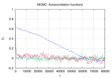
Figure 3: Autocorrelation functions $\rho_{j}(t)$ ($j$ = 1,…,6), calculated for $300\,000$ ensembles of 100 walkers and displayed for the first $80\,000$ ensembles.

Examining the autocorrelation functions, one realizes that a fairly good convergence towards the requested value of 0 is already achieved after a couple of thousands of ensembles, except for parameter 6 which represents the distance of NGC 3077, where it takes about $60\,000$ ensembles. However, afterwards the autocorrelation functions keep varying, mostly within the range of $(-0.1,0.1)$. A detailed discussion of this behaviour is left for Section 6.

As explained in Section 3.5 the ensemble chains serve as input for three-body integration runs into the future. Taking each of the ensembles t = $75\,000$, $100\,000$, …, $300\,000$ as a starting point for continuing the MCMC procedure, we extracted the first 1000 occurences of walkers fulfilling condition COND in each case. This produces ten independent follow-up sets of walkers. As soon as one of the companions is seperated less than 15 kpc (the baryonic radius of M81’s disc) from M81 and does not leave this spatial extension thereafter anymore, we regard this time as the time of the merger process.

In accordance with the statements concerning the behaviour of the autocorrelation functions we present the merger rates within the forthcoming 7 Gyr in Figure 4. Apparently no full convergence is achieved, and the results appear ”to walk around”. As an attempt to achieve meaningful results we calculated the averages of the ten follow-up sets and show them in Figure 5 and Table 4.

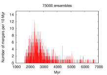
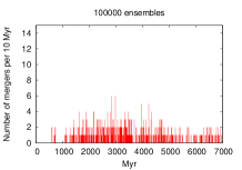
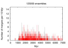
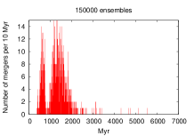
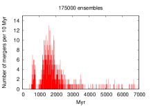
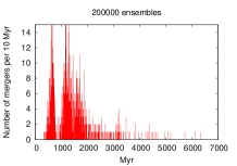
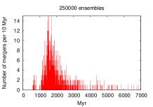
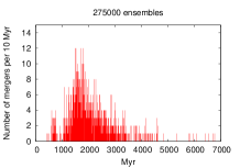
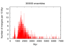
Figure 4: MCMC: Merger rates based on the begin times as of the present displayed for the next 7 Gyr. (For further details refer to the text.)

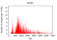
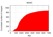
Figure 5: MCMC: Merger rates and cumulated number of mergers displayed for the forthcoming 7 Gyr. In total 1000 walkers were considered by randomly extracting 100 walkers out of each of the ten follow-up sets.

Instead of applying clustering or alike methods in order to achieve full convergence, we decided to employ another statistical method, the genetic algorithm, which overcomes difficulties like the problem of local maxima and the above mentioned one. As we will see, the results obtained there are in good agreement with those obtained by the MCMC method.

5 Statistical Methods II: Genetic Algorithm

General aspects of the genetic algorithm (GA) are explained in detail in Charbonneau (1995). As pointed out there, the major advantage of GA is perceived to be its capability of avoiding local maxima in the process of searching the global maximum of a given function (fitness function). A precise description of the algorithm, especially instructions for the implementation, can also be found in Theis & Kohle (2001).

In our case each open parameter from Table 3 is mapped to a 4-digit string (”gene”) $\left[abcd\right]_{i}$ ($i\in\{1,...,6\}$):

$$P_{i}=(P_{i})_{min}+\left[abcd\right]_{i}\cdot\left[(P_{i})_{max}-(P_{i})_{min}\right]/10\,000\ .$$ (12)

Here the minimum and maximum values for the parameters $P_{i}$ are choosen to be the same as in Section 4.2. All genes together define the genotypes as 6$\times$4-digit strings

$$\ \ \ \ \ \ \ \ \ \ \ \ \ \ \ \ \ \ \ \ \ \ \ \ \framebox{$\left[abcd\right]_{1}...\left[abcd\right]_{6}$}\ ,$$

which, when creating a new generation, undergo the procedures of cross-over, mutation and ranking within a population of $N_{pop}$ genotypes. The first generation is established by randomly creating $N_{pop}$ 6$\times$4-digit strings.

5.1 Definition of the Fitness Function

In contrast to Section 4, where the stretch moves may take walkers outside the ranges specified in Table 1, we need not take care of those ranges explicitly because Eq. 12 a priori guarantees that the distances are confined to their intervals. Otherwise we follow the goal to establish GA evaluations compatible to what has been performed by means of MCMC. Dropping Equation 6 we therefore arrive at the following definition for the fitness function

$$\mathcal{F}(\vec{X}\mid D)=\prod_{i=2}^{3}\ p_{v}(\vec{X})_{i}\cdot P_{C}(\vec{X}\mid D)_{i}\cdot P_{u}(\vec{X}\mid D)_{i}\ ,$$ (13)

where the individual components are taken from Equations 7, 9 and 10. Like in Section 4, $\vec{X}$ denotes the parameter vector while further entities incorporated are indicated by D.

5.2 Results

We generated a set of 1000 solutions fulfilling condition COND. Upon detection of a first solution the GA procedure is being repeated by randomly creating a new population as a starting point, as explained above, until 1000 appropriate three-body orbits are collected.

The fitness function corresponds to the posterior probability density of Section 4. In Figure 6 the merger events occurring within the next 7 Gyr are presented for that model. The comparison of Figures 5 and 6 confirms the statement that both statistical methodes applied, namely MCMC and GA, yield similar results with respect to the merger rates, and key numbers are presented in Table 4.

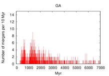
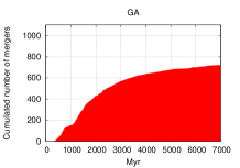
Figure 6: GA: Merger rates and cumulated number of mergers displayed for the forthcoming 7 Gyr, based on a population of 1000 solutions.

	MCMC	GA
solutions not merging within next 7 Gyr	118	278
solutions not merging within next 7 Gyr and:
neither M82 nor N3077 bound to M81 7 Gyr ago	117	276
solutions not merging within next 7 Gyr and:
one companion bound to M81 7 Gyr ago	1	2
solutions for:
M82 and N3077 bound to M81 7 Gyr ago	66	70
longest lifetime from today for:
M82 and N3077 bound to M81 7 Gyr ago	$2.7$ Gyr	$2.8$ Gyr
average lifetime from today for:
M82 and N3077 bound to M81 7 Gyr ago	$1.7$ Gyr	$1.3$ Gyr

Table 4: Key numbers for both statistical methods MCMC and GA, based on populations of 1000 solutions in either case. Actually, the three solutions not merging within the next 7 Gyr where one companion is bound to M81 merge after 7.3 Gyr (MCMC), and 7.8 and 8.2 Gyr (GA).

It is worthwhile to investigate the pre-infall phase space at -7 Gyr. For this purpose we continued the GA-runs until 1000 merging solutions and 1000 solutions not merging were collected. Figure 7 shows the corresponding 3D-plots which were rotated in a way that structures are efficiently visualized. Roughly evaluating Figure 8 for the spatial coordinates and Figure 9 for the velocity components of M82 and NGC 3077 one might draw the conclusion that the phase space volume for the population of the merging solutions fairly exceeds the phase space volume for the population of the non-merging solutions. However, for the population of the merging solutions a higher correlation in phase space is evident from Figure 7 (especially for NGC 3077). Therefore a solid statement regarding the ratio of the phase space volume cannot be readily extracted.

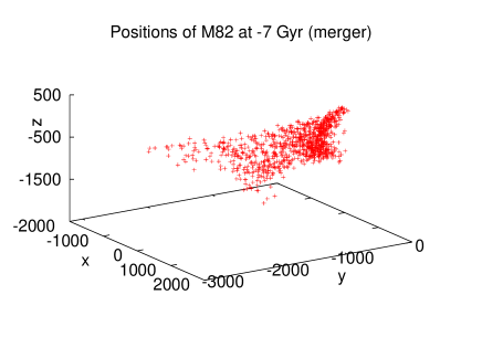
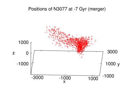
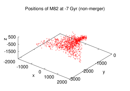
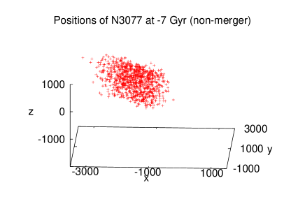
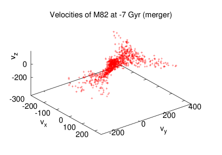
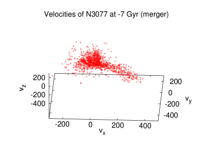
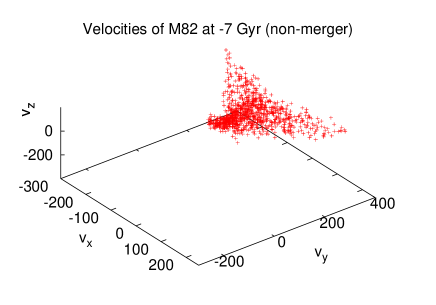
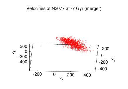
Figure 7: GA: Distribution of the pre-infall phase space at -7 Gyr for M82 and NGC 3077 in today’s M81 reference frame. A population of 1000 solutions merging within the forthcoming 7 Gyr (i.e. within 14 Gyr since -7 Gyr) is displayed in the first and the third row for the coordinates (kpc) and the velocities (pc/Myr), respectively. Accordingly the second and fourth row refer to a population of 1000 solutions not merging.

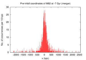
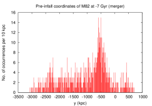
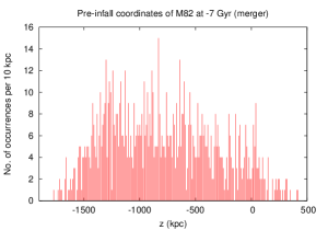
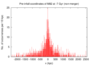
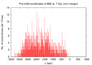
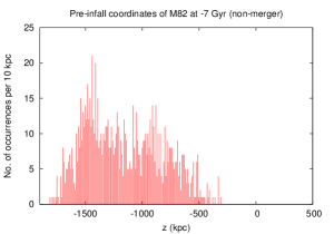
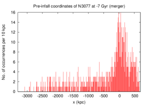
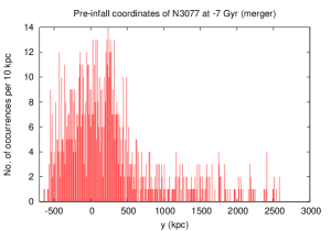
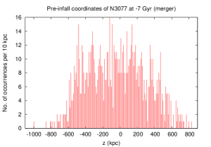
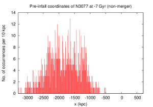
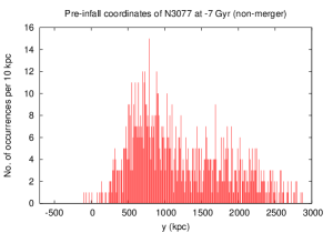
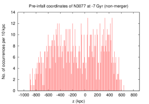
Figure 8: GA: Distribution of the pre-infall coordinates at -7 Gyr for M82 and NGC 3077 in today’s M81 reference frame. A population of 1000 solutions merging within the forthcoming 7 Gyr (i.e. within 14 Gyr since -7 Gyr) is displayed in the first and the third row for M82 and NGC 3077, respectively. Accordingly the second and fourth row refer to a population of 1000 solutions not merging.

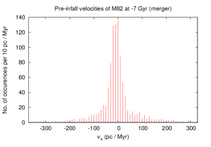
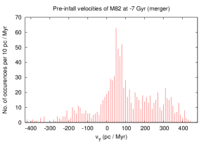
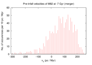
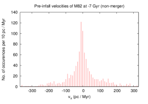
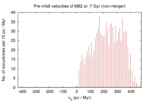
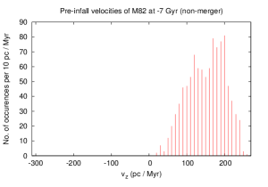
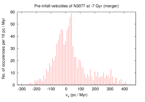
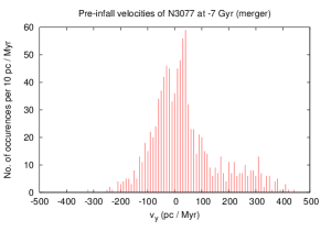
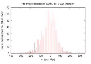
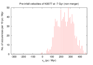
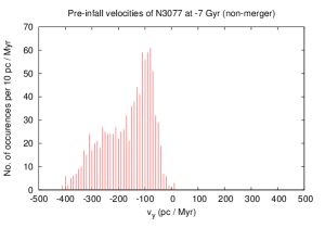
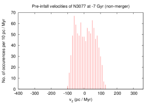
Figure 9: GA: Same as Figure 8, but for the velocity components.

5.3 Extended Fitness Function

In order to facilitate that the GA evaluations preferably generate solutions where at least one of the companions M82 and NGC 3077 is bound to M81, we enhance the fitness function by a function depending on the three-body energy $E$ in the centre-of-mass system before the encounter

$$f_{E}=\left\{\begin{array}[]{ll}1,&E\leq E_{min}/2\ ,\\ \exp\left({-{\displaystyle\frac{\left({E}-{E_{min}/2}\right)^{2}}{2\cdot{(E_{min}/2)}^{2}}}}\right),&E>E_{min}/2\ .\end{array}\right.$$ (14)

Here $E_{min}$ is the minimum three-body energy possible, depending on the particular distances of M82 and NGC 3077 resulting from the genotypes. All together the extended fitness function reads

$$\mathcal{F}_{E}(\vec{X}\mid D)=f_{E}\cdot\mathcal{F}(\vec{X}\mid D)\ .$$ (15)

Thus avoiding the unlikely constellations that both companions are arriving from far distances fulfilling condition COND by collecting solutions with a three-body energy $E$ $\leq$ $0$ in the centre-of-mass system at $-$ 7 Gyr, the resulting merger rates for this fitness function are presented in Figure 10. After $12.6$ Gyr, i.e. $5.6$ Gyr as from today, all solutions will have merged.

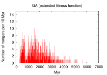
Figure 10: Same as Figure 6, but fitness function $\mathcal{F}_{E}$ (Eq. 15).

5.4 Proper motions

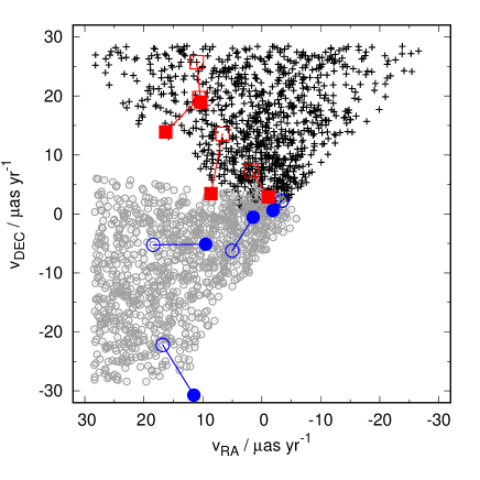
Figure 11: Proper motions of M82 (crosses) and NGC 3077 (open circles) of the GA solutions, all with respect to M81. Left panel: Proper motions in RA and DEC in $\mu\textrm{as\,yr}^{-1}$. Note that the maximum velocity of the solutions in each x,y component is $\pm 500$ $\textrm{km\,s}^{-1}$, corresponding to about $\pm 30$ $\mu\textrm{as\,yr}^{-1}$. The solutions computed with RAMSES are shown as filled squares (M82) and filled circles (NGC 3077) while the corresponding GA solutions are depicted with open symbols, mutually connected by lines. Right panel: The distribution of the absolute velocities, $v_{\textrm{abs}}$ in $\textrm{km\,s}^{-1}$, and the position angles, $\alpha$, in degrees, measured counterclockwise from the North Celestial Pole.

The proper motions of the galaxies are extracted from the available solutions. Since the center-of-mass motion of the M81 group is a free parameter in these calculations the proper motions of M82 and NGC 3077 in the solutions for GA are calculated with respect to M81 at $t=0$ (i.e. present day) in $\mu\textrm{as\,yr}^{-1}$ ($1\,\mu\textrm{as\,yr}^{-1}$ corresponds to 17.2 $\textrm{km\,s}^{-1}$ based on the distance of M81 being 3.62 Mpc). The results are shown in Fig. 11. The velocities are clearly limited to certain directions, at least for higher velocities. In the low-velocity end the direction angles are rather randomly distributed. The distribution of solutions in Fig. 11 allows to place additional constraints on the models with dark matter, once the proper motion of M82 and/or of NGC3077 have been measured. In addition, the solutions computed with RAMSES (Sec. 7) are included as filled squares (M82) and filled circles (NGC 3077) while the corresponding GA solutions are depicted with open symbols, mutually connected by lines. The dynamically self-consistent RAMSES solutions are in good agreement with the GA solutions.

6 Statistical Methods III: Discussion of MCMC vs. GA

As presented in Section 4.3 apparently no full convergence is achieved in our approach of applying the MCMC method to the inner M81 group. The autocorrelation functions keep varying, though at low values (Figure 3), and the merger rates appear ”to walk around” (Figure 4).

We expect that this phenomenon is caused by our choice of the various contributions to the posterior probability density. To be precise, all of them consist partly of a region with a constant value 1, simply because we do not really know, and any procedure defining preferred values there would mean a non-justified interference. As a result, for each open parameter the individual walkers have no direction so long they find themselves in regions of constant value, and unless they are taken out from there again by a stretch move. The missing directions ”where to move to” in regions of constant value probably prevents, in our regard, the MCMC formalism from full convergence.

As already indicated at the end of Section 4.3 we sacrificed on-top methodoligies to MCMC in order to overcome this problem. The transfer to the genetic algorithm, implemented as an additional independent statistical method, turned out to be extremely valuable. For, this formalism apparently delivers stable statistical results under circumstances mentioned above. To establish this assesment we repeated the GA-runs for a second time and present the results in Table 5. Only slight deviations of the merger rates in comparison to the first evaluation are produced by the second one.

However as a matter of fact, at the beginning of our implementation we started with the genetic algorithm. Since, by means of this algorithm, it appeared to be diffcult to generate solutions at all while establishing our concepts we decided to implement the Markov chain Monte Carlo method, too. And in fact we were able to generate solutions by employment of the MCMC method quickly. In our experience, MCMC is the stronger search engine in comparison to GA and therefore helped signifficantly to ”get feet on ground” during the early phase of our project.

To summarize our assessment: Both statistical methods turned out to be very valuable in our regard. MCMC helped to establish the concepts, and at the end GA delivered more stable results.

Table 5: GA: Percentages of mergers for selected periods of time from the present until maximally 7 Gyr. The original GA-evaluations are denoted by #1, and the repitition runs by #2.

Fitness function	GA-run	0-1 Gyr	0-2 Gyr	0-3 Gyr	0-4 Gyr	0-5 Gyr	0-6 Gyr	0-7 Gyr
Eq. 13	#1	15.1%	42.8%	56.6%	63.3%	67.5%	69.8%	72.2%
	#2	13.9%	40.4%	54.0%	61.1%	67.2%	70.9%	73.2%
Eq. 15	#1	22.3%	62.5%	88.8%	96.8%	99.3%	100%	100%
	#2	23.2%	60.9%	86.1%	96.8%	99.2%	99.9%	100%

7 Numerical simulations with RAMSES

	$x$	$y$	$z$	$v_{x}$	$v_{y}$	$v_{z}$
Model 1728-2
M81	153.33	-116.46	499.62	-19.04	16.67	-62.78
M82	268.33	-385.66	-1143.	-38.02	46.11	146.66
NGC3077	-1350.	1439.94	200.22	178.35	-185.38	-32.09
Model 1728-6
M81	13.04	409.78	475.99	-3.82	-49.76	-61.98
M82	-166.98	-1100.0	-1009.9	16.39	139.63	132.02
NGC3077	317.92	534.88	10.61	-18.97	-78.76	-2.57
Model 1728-16
M81	265.72	597.69	256.07	-27.57	-81.71	-31.57
M82	-245.68	-1731.1	-567.83	29.68	230.47	72.63
NGC3077	-719.28	1068.89	61.64	65.10	-132.00	-13.59
Model 1729-633
M81	-18.84	205.98	283.40	-2.07	-12.41	-20.41
M82	68.10	-467.72	-530.50	-13.74	31.52	38.45
NGC3077	-64.56	74.58	-155.10	41.29	-12.12	10.59

Table 6: Initial positions, and velocities of the halos hosting the galaxies M81 (virial mass $=1.17\cdot 10^{12}\,M_{\odot}$), M82 ($5.54\cdot 10^{11}\,M_{\odot}$), and NGC3077 ($2.43\cdot 10^{11}\,M_{\odot}$). The positions are in kpc, the velocities in km/s. Each halo is modelled by particles of $1\cdot 10^{6}\,M_{\odot}$, i.e., the M81 halo contains 1.17 million particles, M82 554,000 particles and NGC3077 243,000 particles.

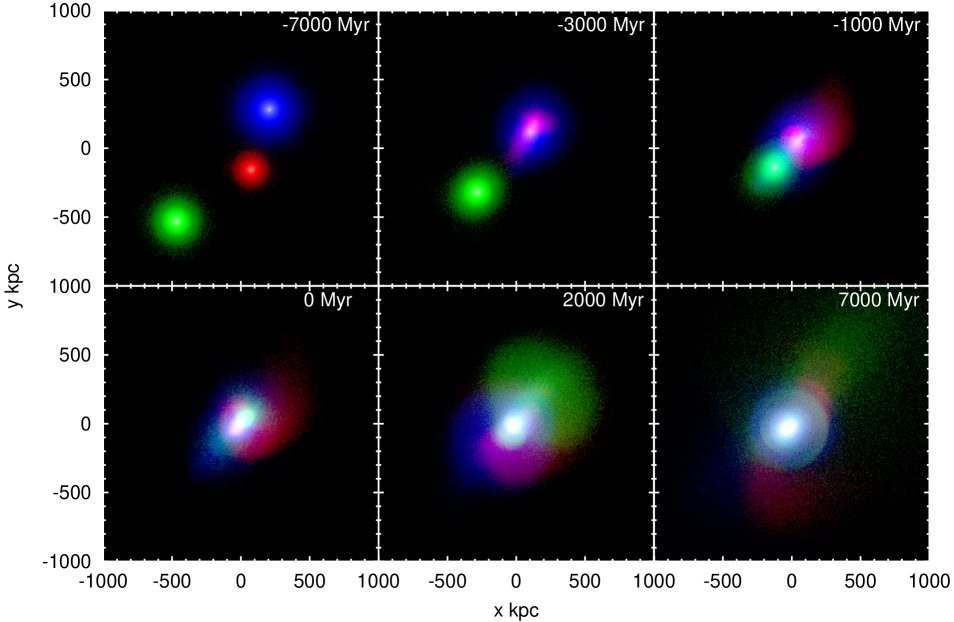
Figure 12: Snapshots of the merging halos of NGC 3077 (red) and M82 (green) with M81 (blue). The initial conditions correspond to model 1729-633. It can be seen that the density centres merge within several Gyr after their first encounter with M81. Both halos lose substantial amounts of mass, partially ejected as tidal streams (NGC 3077), partially as a wide-angle spray cloud (M82). Also shell-like DM structures form (lower right panel).

To validate the semi-analytic approach described in the previous sections, we computed numerical models with the well-tested adaptive mesh refinement (AMR) and particle-mesh code RAMSES (Teyssier, 2002). The halos are set up as NFW profiles (Navarro, Frenk & White, 1996) as in the semi-analytic model described in Section 3.4. The virial masses are the same as in the semi-analytic model (see Tables 1 and 2). The total masses are taken as the DM halo masses, i.e. neglecting the baryonic content. The initial positions and velocities are listed in in Table 6. In total 1.967 million particles are used for the models shown here, with each particle representing $10^{6}\,M_{\odot}$. Each simulation takes between about 10 and 30 hours with 32 parallel threads used. Additional runs with 196,700 and 19,670 particles have been performed to confirm the models to be essentially independent of the particle number, which is indeed the case. The halos are allowed to settle for several Gyr before being included in the initial conditions for the simulations. The position of each halo is represented by the density centre calculated via the method described by Casertano & Hut (1985). The density centre method rather than the centre of mass has been chosen to determine the positions and mutual distances of the halos since the in-falling halos lose large amounts of mass upon encounter (see Fig. 12). The resulting steady shift of the centre of mass would render its position useless for the purpose of this study. In addition, the density centres are the best representations of the positions of the embedded galaxies which can be observed today.

The models studied in this section correspond to the 3-body genetic algorithm solutions No. 1728-2, 1728-6, 1728-16, and 1729-633 for fitness function Eq. 13, and to the solutions No. 1750-314, 1750-224, 1750-423, and 1750-445 for the extended fitness function Eq. 15. They are shown on the left side of Figure 13 and 14, respectively, and were chosen randomly from the full set of GA solutions.

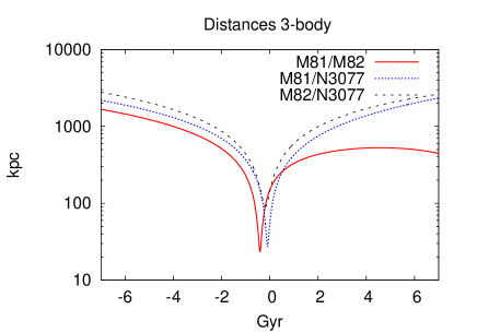
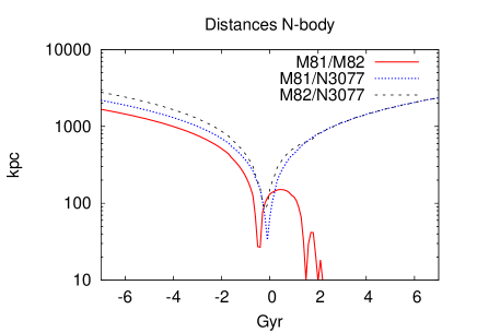
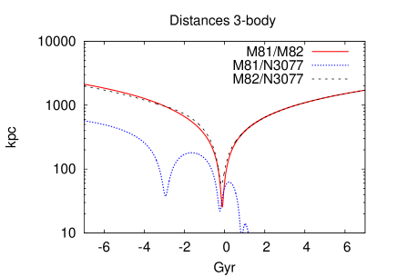
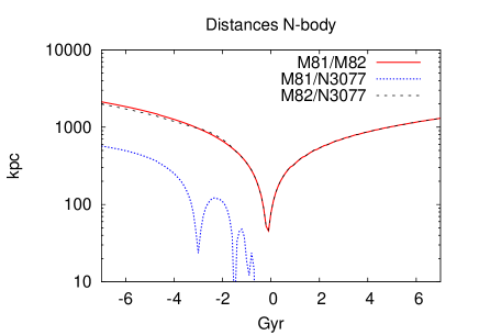
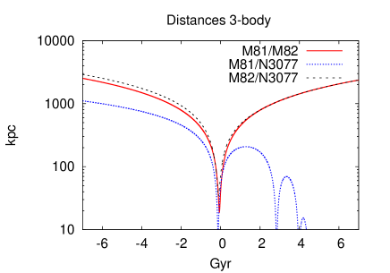
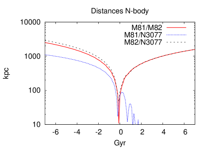
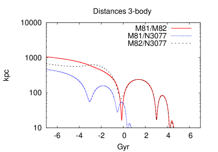
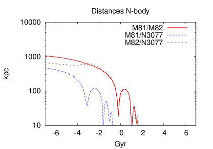
Figure 13: Comparison between the results obtained by the 3-body model (left) and the N-body calculations (right). Four solutions were selected randomly out of the population created by the GA method, fitness function Eq. 13. First row (solution 1728-2): no merger within the forthcoming 7 Gyr. Second row (1728-6): rapid merger ($0.8$ Gyr). Third row (1728-16): merger after $4.2$ Gyr. Fourth row (1729-633): both companions are merging with M81.

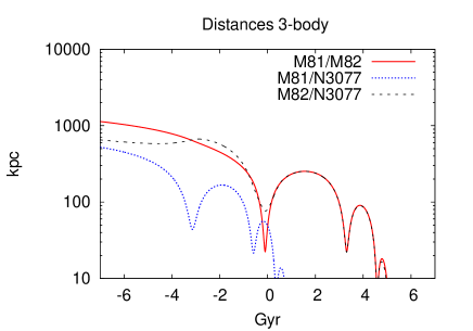
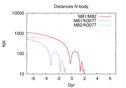
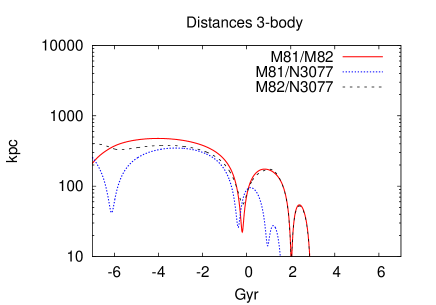
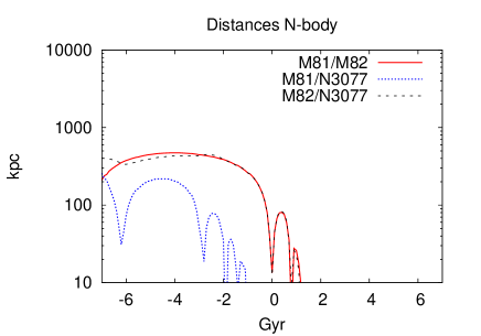
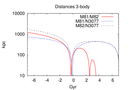
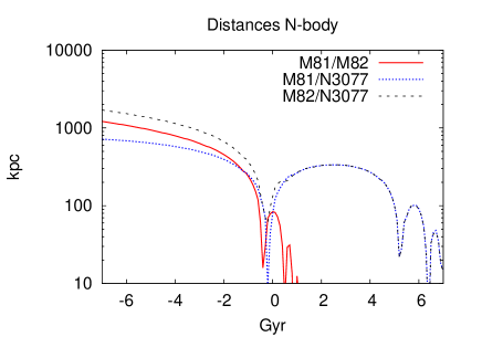
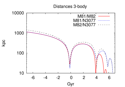
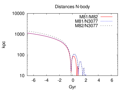
Figure 14: Same as Figure 13, but four solutions generated by means of the extended fitness function Eq. 14. First row (solution 1750-314): most rapid merger ($0.3$ Gyr). Second row (1750-224): merger after $1.5$ Gyr. Third row (1750-423): merger after $3.5$ Gyr. Fourth row (1750-445): latest merger after $5.6$ Gyr.

7.1 Results

Figure 12 shows snapshots of the encounter leading to the merger of all halos for model 1729-633. As can be seen the dynamical friction causes the in-falling halos of NGC 3077 (red) and M82 (green) to decelerate quickly and merge with the halo of M81 (blue) after a few oscillations. Figure 13 and Figure 14 show the mutual distances for the galaxies. The left-hand frames depict the results from the 3-body GA calculations while the right columns contain the results of the RAMSES $N$-body simulations. The solid line refers to the distances of M82 to M81, the dotted line those of NGC3077 to M81, and the distances between the minor components M82 and NGC3077 are shown by the dashed line. All mutual distances follow a time evolution very similar to the semi-analytic solution. The RAMSES $N$-body computations lead to slightly to substantially lower post-encounter velocities compared to the semi-analytical 3-body calculations. The reason for this is probably the large mass loss along two dense tidal streams which causes a larger energy loss during the encounter. This seems to contradict Boylan-Kolchin et al. (2008) who predict longer merger times especially for large satellite-to-host mass ratios compared to the results of semi-analytic calculations using Chandrasekhar’s formula. In the Coulomb logarithm model used in the previous sections, on the other hand, the merger timescale for the semi-analytic calculations are slightly longer than in the RAMSES simulation rendering that Coulomb logarithm more conservative. The halos merge as fast as in GA and even faster in the right panel, thus validating the GA solutions. There are some additional effects to be noted:

• The in-falling halos of M82 and NGC 3077 suffer substantial mass loss during the merging process. The ejected DM forms tidal streams in almost opposite directions (NGC 3077, see Fig. 12) as well as a wide spray (M82), depending on the encounter parameters.

• The density centres of M82 and NGC 3077 first oscillate around M81 and then merge shortly after the present (marked by time $=0$).

• All halos merge faster or lose more kinetic energy in the full $N$-body computations than in the semi-analytic model (right panels of Fig. 13). This emphasises the importance of dynamical friction.

8 Conclusions

We summarize the results obtained as follows:

• Solutions which fulfill the broad criterion COND and where the three galaxies have not merged at the present do exist within the LCDM model.

• The treatment of the inner M81 group by high-resolution simulations of live self-consistent systems presented in Section 7 confirms that the simplified three-body model of rigid NFW halos serves as a physical basis for our statistical evaluations. The semi-analytical approach for treating dynamical friction turns out to be a cautious estimate as the comparison with orbits obtained in Section 7 show that in full N-body calculations the galaxies merge even more efficiently due to dynamical friction and as a result of energy removal through expulsion of dark matter particles as tidal material.

• Two independent statistical methods (Section 4 and Section 5) yield results in good agreement with each other.

• According to these results, only $7\%$ of all initial conditions of either statistical population reflect pre-infall three-body bound states at $-7$ Gyr fulfilling condition COND. Such three-body bound states merge rapidly in the near cosmological future, the average future lifetimes being given by $1.7$ Gyr (according to the MCMC search) and $1.3$ Gyr (according to the GA search). The longest lifetimes are given by $2.7$ Gyr for MCMC and $2.8$ Gyr for the GA search (see Table 4).

• All solutions (which fulfill the condition COND by the requirement to be a solution) of both statistical populations not merging within the next 7 Gyr from today comprise orbits where both companions initially are not bound to M81 and arrive from a far distance.

• For the sake of avoiding those constellations where both companions arrive nearly simeltaneously from a far distance, an extended fitness function searching for states of negative pre-infall three-body energy (see Section 5.3) delivers mostly results where one companion is bound to M81 while the other one arrives from a far distance. The longest future lifetime for this population is $5.6$ Gyr.

Thus, using three-body restricted simulations that model dynamical friction on dark matter halos, which are in fact confirmed by full N-body models, we find that the three inner galaxies in the M81 group are likely to merge within the next 1-2 Gyr. If we assume that the constraint COND is right then it is very likely that both or at least one of the two dwarfs started out from far away and was not bound at $-7\,$Gyr. For a bound system which survives for a longer time-span (into the past and also into the future) we either have to relax the condition COND, or if COND is true, then the amount of DM of the three galaxies assumed in this study needs to be reduced significantly. Additional constraints will be available with relative proper motion measurements within the M81 group of galaxies which will significantly reduce the allowed range of solutions and by taking into account the tidally displaced gas distribution in the M81 system.

Other evidence for dynamical friction through dark matter halos or the lack thereof has been discussed, and it is worth to briefly mention it here. The observed compact groups of galaxies would also require highly tuned initial conditions such that its members are all together about 1–2 Gyr from merging (see e.g. Sohn et al. 2015), thus confirming our results regarding the inner M81 group of galaxies. Measured proper motions of the satellite galaxies of the Milky Way provide additional constraints (Angus et al., 2011).

Appendix A Program Development

Apart from Section 7 (Numerical Simulations with RAMSES), all numerical computations were realized within the frame of SAP’s Development Workbench, utilizing the programming language ABAP and the related debugging facilities, the Repository (SE11) for easy creation of the requested statistical databases, and their evaluation (SE16, REUSE_ALV_GRID_DISPLAY). In comparison to development environments like C++ or FORTRAN, the ABAP Development Workbench facilitated a program development time at least two or three times faster. However aspects like the performance of floating point calculations, or easy linkage to mathematical standard libraries need to be improved for the sake of full acceptance in the world of numerical programming.

Appendix B Abbreviations

ABAP:	SAP’s programming language
COND:	Condition specified in Section 3.5
DM:	Dark matter
GA:	Genetic algorithm
MCMC:	Markov chain Monte Carlo
MW:	Our galaxy (Milky Way)
NED:	NASA/IPAC extragalactic database
NFW:	Navarro, Frenk & White profile
NTB:	North tidal bridge
POS:	Plane of sky
LCDM:	Standard dark-energy plus cold-dark-matter
	model of cosmology
STB:	South tidal bridge

Appendix C Numerical Solution of the three-body orbits

The Hamilton equations, extended by the non-conservative forces $\vec{F}^{DF}_{ij}$ due to dynamical friction, have been integrated numerically in the centre of mass system of the three galaxies M81, M82 and NGC 3077, represented by the indices $i,j$ = 1,2,3, respectively. Using Cartesian coordinates (index $k$ = 1,2,3), they read in the 18-dimensional phase space (the advantage of reducing this dimension to 12 by the use of Jacobi variables is being cancelled by the disadvantage of complicating the structure of the equations):

$$\frac{d}{dt}{(\vec{x}_{i})}_{k}=\frac{{(\vec{p}_{i})}_{k}}{m_{i}}\ ,$$

$$\frac{d}{dt}{(\vec{p}_{i})}_{k}=\sum_{j\neq i}\left[{-\ \frac{\partial}{{\partial{(x_{i})}_{k}}}}V_{ij}\ +\ (\vec{F}^{DF}_{ij})_{k}\ -\ (\vec{F}^{DF}_{ji})_{k}\right]\ .$$

The DF force on galaxy $i$ moving in the DM halo of galaxy $j$ is given by $\vec{F}^{DF}_{ij}$. Vice versa, the DF force on galaxy $j$ moving in the DM halo of galaxy $i$ appears in the equation of motion for galaxy $i$ via actio est reactio with reversed sign.

The potential energies $V_{ij}$ betweeen the galaxies are detemined by the NFW density profiles given by Eq. 3 and Table 2. At distances where the DM halos of the galaxies are completely separated the gravitational force is given by Netwon’s law for point masses. In case of overlapping DM halos the potential energy between two halos $i,j$ is numerically calculated by reducing halo $j$ to volume elements $h^{3}$ with $h~{}=~{}1~{}kpc$ and summation of those volume elements in the potential $\Phi_{i}$ of halo $i$:

$$\Phi_{i}(s_{i})=\left\{\begin{array}[]{ll}-\ G\ \int\limits_{0}^{s_{i}}\ \frac{m_{i}(r_{i})}{{r_{i}}^{2}}\ dr_{i}\ \ +\ const,&s_{i}\leq R_{200_{i}}\ ,\\ \\ -\ G\ \frac{m_{i}}{s_{i}}\ ,&s_{i}>R_{200_{i}}\ ,\\ \end{array}\right.$$

$const$ being determined by continous transition at $R_{200_{i}}$,

$$V_{ij}(r_{ij})=\left\{\begin{array}[]{ll}\sum_{n}\Phi_{i}(s_{i_{n}})\ \rho_{j}(s_{j_{n}})\ h^{3},&r_{ij}\leq R_{200_{i}}+R_{200_{j}}\ ,\\ \\ -\ G\ \frac{m_{i}m_{j}}{r_{ij}}\ ,&r_{ij}>R_{200_{i}}+R_{200_{j}}\ ,\\ \end{array}\right.$$

with $s_{i}$ and $s_{j}$ denoting the distances of volume element $h^{3}$ to the centres of halos $i$ and $j$, respectively. For overlapping halos the derivative of the potential energies are then obtained numerically. The first row of Figure 2 visually proves the stability of our numerical computations and their accuracy, which of course additionally was checked by comparing the results for varying seizes of the volume elements.

Furthermore, incorporating the dynamical friction between the DM halos of the three galaxies according to Eq. 1, first of all one has to replace $\vec{\textbf{v}}_{M}$ by the relative velocities

$$\vec{\textbf{v}}_{ij}=\vec{\textbf{v}}_{i}-\vec{\textbf{v}}_{j}\ .$$

Employing actio est reactio we find

$$\frac{d}{dt}\vec{\textbf{v}}_{ij}=\frac{d}{dt}\left(\vec{\textbf{v}}_{i}-\vec{\textbf{v}}_{j}\right)=\frac{1}{\mu_{ij}}\frac{d\vec{p}_{i}}{dt}\ \ \ \rm{with}\ \ \ \frac{1}{\mu_{ij}}=\frac{1}{m_{i}}+\frac{1}{m_{j}}\ ,$$

with the result for Chandrasekhar’s formula:

$$\vec{F}^{DF}_{ij}=-\mu_{ij}\frac{4{\pi}G^{2}{m_{i}}{\rho_{j}}}{\textnormal{v}_{ij}^{3}}\ \textnormal{ln}{\Lambda}_{ij}\left[\textnormal{erf}(X_{j})-\frac{2X_{j}}{\sqrt{{\pi}}}\textnormal{e}^{-X_{j}^{2}}\right]{\vec{\textbf{v}}_{ij}}\ .$$

The dependence of the Coulomb logarithm on the masses (see Eq. 2) is indicated by $\Lambda_{ij}$ and the entity $X_{j}$ is determined by the relative velocity $\textnormal{v}_{ij}$ and the dispersion $\sigma$ of galaxy $j$.

However, this equation is based on the assumption of Maxwellian type velocity distributions which is not the case for NFW profiles. Since most of the contribution to dynamical friction is certainly caused by the immediate vicinity of an intruder we replace the dispersion $\sigma$ by the distance dependent circular speed $v_{c}$

$$X_{j}(s_{j})=\textnormal{v}_{ij}/v_{c_{j}}(s_{j})\ ,$$

at a distance $s_{j}$ from the halo centre of galaxy $j$. Similarly to the potential energies, here the total DF force between two overlapping halos is numerically obtained by reducing the DM halo $i$ to volume elements $h^{3}$ with distance $s_{i}$ to its centre, and computing the sum over them:

$$\vec{F}^{DF}_{ij}=-\mu_{ij}\frac{4{\pi}G^{2}}{\textnormal{v}_{ij}^{3}}f_{ij}\ {\vec{\textbf{v}}_{ij}}\ ,$$

with

$$f_{ij}=\sum_{n}\rho_{i}(s_{i_{n}})h^{3}\ \rho_{j}(s_{j_{n}})\ \textnormal{ln}{\Lambda}_{ij}\left[\textnormal{erf}(X_{j})-\frac{2X_{j}}{\sqrt{{\pi}}}\textnormal{e}^{-X_{j}^{2}}\right]$$

and

$$\textnormal{ln}{\Lambda}_{ij}(s_{j})=\textnormal{ln}\left[1+m_{j}(s_{j})/m_{i}\right]\ .$$

For the sake of a better performance, the potential energies $V_{ij}$ and the functions $f_{ij}$ where calculated once on a grid of appropriate base points and interpolated when numerically solving the equations of motion.

For the computation of the differential equations we implemented methods for the Runge-Kutta and leapfrog integration schemes. In order to save performance, a practical variable step size method for the solution of the Hamilton equations was created by adapting the step size according to the minimum of the, at the corresponding point of time, given distances between M81, M82 and NGC 3077, denoted as $d_{min}$. For the leapfrog integration scheme it reads:

$$\Delta t=\left\{\begin{array}[]{ll}0.1\ \rm{Myr},&d_{min}\leq 1\ \rm{kpc}\\ 0.1\ (d_{min}/\rm{kpc})\ \rm{Myr},&1\ \rm{kpc}<d_{min}\leq 1000\ \rm{kpc}\\ 100\ \rm{Myr},&d_{min}>1000\ \rm{kpc}\ .\end{array}\right.$$

This method was thoroughly tested by comparing solutions achieved in that way with integration runs using fixed small stepsizes employing the leapfrog and the Runge-Kutta integration schemes.

Appendix D The Markov Chain Monte Carlo Method

A Markov chain ensemble consists of $N_{L}$ walkers represented by vectors $\vec{X}_{l}\in{\textrm{R}}^{N_{P}}$ with $l\in\{1,...,N_{L}\}$ and $N_{P}$ denoting the dimension of the parameter space. In our case we have $\vec{X}_{l}=\left(P_{1}...P_{6}\right)$ (see Table 3). For the evolution of an affine-invariant Markov chain of ensembles by means of the Metropolis-Hastings algorithm we implemented the stretch move as explained in Foreman-Mackey et al. (2013), which is based on the determination of the posterior probability density for one walker

$$\pi(\vec{X}\mid D)=const\cdot p(\vec{X})\cdot P(\vec{X}\mid D)\ .$$ (16)

In our regard the normalization factor $const$ is not relevant because only the ratio of the posterior probability densities for two walkers have to be determined when performing the stretch move. $p(\vec{X})$ denotes the prior distribution, and the likelihood function $P(\vec{X}\mid D)$ may not only depend on the parameters $P_{1}$ to $P_{6}$, but on further entities symbolized by $D$, too.

The mean value of parameter $P_{j}$ for sample $t$ is given by

$$f_{j}(\vec{X}(t))=\frac{1}{N_{L}}\sum_{l=1}^{N_{L}}{\left[\vec{X}_{l}(t)\right]}_{j}\ ,$$ (17)

and dealing with a total number of $N_{T}$ samples we have for the overall mean value:

$$<f_{j}>=\frac{1}{N_{T}}\sum_{t=1}^{N_{T}}f_{j}(\vec{X}(t))\ .$$ (18)

For sufficiently large values of $N_{T}$ the autocovariance function for parameter $P_{j}$ can be approximated by

$$C_{j}(t)\approx\frac{1}{{N_{T}}-t}\ \times$$ (19)

$$\times\sum_{t^{\prime}=1}^{{N_{T}}-t}{\left(f_{j}(\vec{X}(t^{\prime}+t))-<f_{j}>\right)}{\left(f_{j}(\vec{X}(t^{\prime}))-<f_{j}>\right)},$$

and we finally arrive at estimates for the autocorrelation functions,

$$\rho_{j}(t)=\frac{C_{j}(t)}{C_{j}(0)}\ ,$$ (20)

and the integrated autocorrelation times

$$\tau_{j}\approx 1+2\sum_{t=1}^{N_{T}}\rho_{j}(t)\ .$$ (21)

References

- Angus et al. (2011) Angus G. W., Diaferio A., Kroupa P., 2011, MNRAS, 416, 1401
- Appleton et al. (1981) Appleton P. N., Davies R. D., Stephenson R., 1981, MNRAS, 195, 327
- Barnes (1998) Barnes J. E., 1998, in Saas-Fee Advanced Course 26. Lecture Notes 1996 Vol. XIV of Swiss Society for Astrophysics and Astronomy, Galaxies: Interactions and Induced Star Formation, Saas-Fee Advanced Course 26. Lecture Notes 1996, Springer Verlag Berlin/Heidelberg, p.275
- Behroozi et al. (2013) Behroozi P. S., Wechsler R. H., Conroy C., 2013, ApJ, 770, 57
- Binney & Tremaine (2008) Binney J., Tremaine S., 2008, Galactic Dynamics, 2 edn. Princeton University Press
- Boylan-Kolchin et al. (2008) Boylan-Kolchin M., Ma C.-P., Quataert E., 2008, MNRAS, 383, 93
- Casertano & Hut (1985) Casertano S., Hut P., 1985, ApJ, 298, 80
- Chandrasekhar (1942) Chandrasekhar S., 1942, Principles of Stellar Dynamics. The University of Chicago Press
- Chandrasekhar (1943) Chandrasekhar S., 1943, ApJ, 97, 255
- Charbonneau (1995) Charbonneau P., 1995, ApJS, 101, 309
- Cottrell (1977) Cottrell G., 1977, MNRAS, 178, 577
- De Propris et al. (2014) De Propris R., Baldry I. K., Bland-Hawthorn J., Brough S., Driver S. P., Hopkins A. M., Kelvin L., Loveday J., Phillipps S., Robotham A. S. G., 2014, MNRAS, 444, 2200
- Famaey & McGaugh (2012) Famaey B., McGaugh S. S., 2012, Living Reviews in Relativity, 15, 10
- Foreman-Mackey et al. (2013) Foreman-Mackey D., Hogg D. W., Lang D., Goodman J., 2013, PASP, 125, 306
- Goodman & Weare (2010) Goodman J., Weare J., 2010, Comm. App. Math. Comp. Sci., 5, 65
- Gottesman & Weliachev (1977) Gottesman S. T., Weliachev L., 1977, ApJ, 211, 47
- Jiang et al. (2008) Jiang C. Y., Jing Y. P., Faltenbacher A., et al. 2008, ApJ, 675, 1095
- Koyama (2016) Koyama K., 2016, Reports on Progress in Physics, 79, 046902
- Kroupa (2015) Kroupa P., 2015, Canadian Journal of Physics, 93, 169
- Lena et al. (2014) Lena D., Robinson A., Marconi A., Axon D. J., Capetti A., Merritt D., Batcheldor D., 2014, ApJ, 795, 146
- Macciò et al. (2007) Macciò A. V., Dutton A. A., van den Bosch F. C., Moore B., Potter D., Stadel J., 2007, MNRAS, 378, 55
- Navarro et al. (1995) Navarro J. F., Frenk C. S., White S. D. M., 1995, MNRAS, 275, 720
- Navarro et al. (1996) Navarro J. F., Frenk C. S., White S. D. M., 1996, ApJ, 462, 563
- Petsch & Theis (2008) Petsch H. P., Theis C., 2008, AN, 329, 1046
- Privon et al. (2013) Privon G. C., Barnes J. E., Evans A. S., et al 2013, ApJ, 771, 120
- Richtler et al. (2011) Richtler T., Salinas R., Misgeld I., Hilker M., Hau G. K. T., Romanowsky A. J., Schuberth Y., Spolaor M., 2011, A&A, 531, A119
- Sachdeva & Saha (2016) Sachdeva S., Saha K., 2016, ApJ, 820L, 4S
- Samurović (2006) Samurović S., 2006, Serb. Astron. J., 173, 35
- Samurović (2014) Samurović S., 2014, A&A, 570, A132
- Samurović & Ćirković (2008) Samurović S., Ćirković M. M., 2008, A&A, 488, 873
- Samurović & Danziger (2005) Samurović S., Danziger I. J., 2005, MNRAS, 363, 769
- Sohn et al. (2015) Sohn J., Hwang H. S., Geller M. J., Diaferio A., Rines K. J., Lee M. G., Lee G.-H., 2015, Journal of Korean Astronomical Society, 48, 381
- Teyssier (2002) Teyssier R., 2002, A&A, 385, 337
- Theis & Kohle (2001) Theis C., Kohle S., 2001, A&A, 370, 365
- Thomasson & Donner (1993) Thomasson M., Donner K. J., 1993, A&A, 272, 153
- Thomson et al. (1999) Thomson R. C., Laine S., Turnbull A., 1999, in Barnes J. E., Sanders D. B., eds, Galaxy Interactions at Low and High Redshift Vol. 186 of IAU Symposium, Towards an Interaction Model of M81, M82 and NGC 3077. p. 135
- van der Hulst (1979) van der Hulst J. M., 1979, A&A, 75, 97
- Yun (1999) Yun M. S., 1999, in Barnes J. E., Sanders D. B., eds, Galaxy Interactions at Low and High Redshift Vol. 186 of IAU Symposium, Tidal Interactions in M81 Group. p. 81
- Yun et al. (1993) Yun M. S., Ho P. T. P., Lo K., 1993, ApJ, 411, L17
- Yun et al. (1994) Yun M. S., Ho P. T. P., Lo K., 1994, Nat, 372, 530
- Zhao et al. (2013) Zhao H., Famaey B., Lüghausen F., Kroupa P., 2013, A&A, 557, LL3