On spectral partitioning of signed graphs

Abstract

We argue that the standard graph Laplacian is preferable for spectral partitioning of signed graphs compared to the signed Laplacian. Simple examples demonstrate that partitioning based on signs of components of the leading eigenvectors of the signed Laplacian may be meaningless, in contrast to partitioning based on the Fiedler vector of the standard graph Laplacian for signed graphs. We observe that negative eigenvalues are beneficial for spectral partitioning of signed graphs, making the Fiedler vector easier to compute.

1 Background and Motivation

Spectral clustering groups together related data points and separates unrelated data points, using spectral properties of matrices associated with the weighted graph, such as graph adjacency and Laplacian matrices; see, e.g., [chapter_sc, Luxburg2007, Meila01learningsegmentation, ng2002spectral, Shi:2000:NCI:351581.351611, doi:10.1137/0611030, Bolla2013, 7023445]. The graph Laplacian matrix is obtained from the graph adjacency matrix that represents graph edge weights describing similarities of graph vertices. The graph weights are commonly defined using a function measuring distances between data points, where the graph vertices represent the data points and the graph edges are drawn between pairs of vertices, e.g., if the distance between the corresponding data points has been measured.

Classical spectral clustering bisections the graph according to the signs of the components of the Fiedler vector defined as the eigenvector of the graph Laplacian, constrained to be orthogonal to the vector of ones, and corresponding to the smallest eigenvalue; see [fiedler1973algebraic].

Some important applications, e.g., Slashdot Zoo [Kunegis:2009:SZM:1526709.1526809] and correlation [bansal2004] clustering, naturally lead to signed graphs, i.e., with both positive and negative weights. Negative values in the graph adjacency matrix result in more difficult spectral graph theory; see, e.g., [doi:10.1137/130913973].

Applying the original definition of the graph Laplacian to signed graphs breaks many useful properties of the graph Laplacian, e.g., leading to negative eigenvalues, making the definition of the Fiedler vector ambivalent. The row-sums of the adjacency matrix may vanish, invalidating the definition of the normalized Laplacian. These difficulties can be avoided in the signed Laplacian, e.g., [2016arXiv160104692G, Kolluri:2004:SSR:1057432.1057434, doi:10.1137/1.9781611972801.49], defined similarly to the graph Laplacian, but with the diagonal entries positive and large enough to make the signed Laplacian positive semi-definite.

We argue that the original graph Laplacian is a more natural and beneficial choice, compared to the popular signed Laplacian, for spectral partitioning of signed graphs. We explain why the definition of the Fiedler vector should be based on the smallest eigenvalue, no matter whether it is positive or negative, motivated by the classical model of transversal vibrations of a mass-spring system, e.g., [gould, Demmel99], but with some springs having negative stiffness, cf. [AKnegativePatent].

Inclusions with negative stiffness can occur in mechanics if the inclusion is stored with energy [natureNegativeStiffness2001], e.g., pre-stressed and constrained. We design inclusions with negative stiffness by pre-tensing the spring to be repulsive [CHRONOPOULOS201748]. Allowing only the transversal movement of the masses, as in [Demmel99], gives the necessary constraints.

The resulting eigenvalue problem for the vibrations remains mathematically the same, for the original graph Laplacian, no matter if some entries in the adjacency matrix of the graph are negative. In contrast, to motivate the signed Laplacian, the “inverting amplifier” model in [doi:10.1137/1.9781611972801.49, Sec. 7] uses a questionable argument, where the sign of negative edges changes in the denominator of the potential, but not in its numerator

Turning to justification of spectral clustering via relaxation, we compare the standard “ratio cut,” e.g., [Meila01learningsegmentation, ng2002spectral], and “signed ratio cut” of [doi:10.1137/1.9781611972801.49], noting that minimizing the signed ratio cut may amplify cutting positive edges. We illustrate the behavior of the Fiedler vector for an intuitively trivial case of partitioning a linear graph modelled by vibrations of a string. We demonstrate numerically and analyze deficiencies of the signed Laplacian vs. the standard Laplacian for spectral clustering on a few simple examples.

Graph-based signal processing introduces eigenvectors of the graph Laplacian as natural substitutions for the Fourier basis. The construction of the graph Laplacian of [knyazev2015conjugate] is extended in [knyazev2015edge] to the case of some negative weights, leading to edge enhancing denoising of an image that can be used as a precursor for image segmentation along the edges. We extend the use of negative weights to graph partitioning in the present paper.

The rest of the paper is organized as follows. We introduce spectral clustering in Section 2 via eigendecomposition of the graph Laplacian. Section 3 deals with a simple, but representative, example—a linear graph,—and motivates spectral clustering by utilizing properties of low frequency mechanical vibration eigenmodes of a discrete string, as an example of a mass-spring model. Negative edge weights are then naturally introduced in Section 4 as corresponding to repulsive springs, and the effects of negative weights on the eigenvectors of the Laplacian are informally predicted by the repulsion of the masses connected by the repulsive spring. In Section 5, we present simple motivating examples, discuss how the original and signed Laplacians are introduced via relaxation of combinatorial optimization, and numerically compare their eigenvectors and gaps in the spectra. Possible future research directions are spotlighted in Section LABEL:s:future.

2 Brief introduction to spectral clustering

Let entries of the real symmetric $N$-by-$N$ data similarity matrix $W$ be called weighs and the matrix $D$ be diagonal, made of row-sums of the matrix $W$. The matrix $W$ may be viewed as a matrix of scores that digitize similarities of pairs of $N$ data points. Similarity matrices are commonly determined from their counterparts, distance matrices, which consist of pairwise distances between the data points. The similarity is small if the distance is large, and vice versa. Traditionally, all the weighs/entries in $W$ are assumed to be non-negative, which is automatically satisfied for distance-based similarities. We are interested in clustering in a more general case of both positive and negative weighs, e.g., associated with pairwise correlations of the data vectors.

Data clustering is commonly formulated as graph partitioning, defined on data represented in the form of a graph $G=(V,\,E,\,W)$, with $N$ vertices in $V$ and $M$ edges in $E$, where entries of the $N$-by-$N$ graph adjacency matrix $W$ are weights of the corresponding edges. The graph is called signed if some edge weighs are negative. A partition of the vertex set $V$ into subsets generates subgraphs of $G$ with desired properties.

A partition in the classical case of non-weighted graphs minimizes the number of edges between separated sub-graphs, while maximizes the number of edges within each of the sub-graphs. The goal of partitioning of signed graphs, e.g., into two vertex subsets $V_{1}$ and $V_{2}$, can be to minimize the total weight of the positive cut edges, while at the same time to maximize the absolute total weight of the negative cut edges. For uniform partitioning, one also needs to well-balance sizes/volumes of $V_{1}$ and $V_{2}$. Traditional approaches to graph partitioning are combinatorial and naturally fall under the category of NP-hard problems, solved using heuristics, such as relaxing the combinatorial constraints.

Data clustering via graph spectral partitioning is a state-of-the-art tool, which is known to produce high quality clusters at reasonable costs of numerical solution of an eigenvalue problem for a matrix associated with the graph, e.g., $Lx=\lambda x$ for the graph Laplacian matrix $L=D-W$, where the scalar $\lambda$ denotes the eigenvalue corresponding to the eigenvector $x$. To simplify our presentation for the signed graphs, we mostly avoid the normalized Laplacian $D^{-1}L=I-D^{-1}W$, where $I$ is the identity matrix, e.g., since $D$ may be singular.

The Laplacian matrix $L$ always has the number $0$ as an eigenvalue; and the column-vector of ones is always a trivial eigenvector of $L$ corresponding to the zero eigenvalue. Since the graph adjacency matrix $W$ is symmetric, the graph Laplacian matrix is also symmetric, so all eigenvalues of $L$ are real and the various eigenvectors can be chosen to be mutually orthogonal. All eigenvalues are non-negative if the graph weights are all non-negative.

A nontrivial eigenvector of the matrix $L$ corresponding to smallest eigenvalue $\lambda$ of $L$, commonly called the Fiedler vector after the author of [fiedler1973algebraic], bisects the graph $G$ into only two parts, according to the signs of the entries of the eigenvector. Since the Fiedler vector, as any other nontrivial eigenvector, is orthogonal to the vector of ones, it must have entries of opposite signs, thus, the sign-based bisection always generates a non-trivial two-way graph partitioning. We explain in Section 3, why such a partitioning method is intuitively meaningful.

A multiway spectral partitioning is obtained from “low frequency eigenmodes,” i.e., eigenvectors corresponding to a cluster of smallest eigenvalues, of the Laplacian matrix $L.$ The cluster of (nearly)-multiple eigenvalues naturally leads to the need of considering a Fiedler invariant subspace of $L$, spanned by the corresponding eigenvectors, extending the Fiedler vector, since the latter may be not unique or well defined numerically in this case. The Fiedler invariant subspace provides a geometric embedding of graph’s vertices, reducing the graph partitioning problem to the problem of clustering of a point cloud of embedded graph vertices in a low-dimensional Euclidean space. However, the simple sign-based partitioning from the Fiedler vector has no evident extension to the Fiedler invariant subspace.

Practical multiway spectral partitioning can be performed using various competing heuristic algorithms, greatly affecting the results. While these same heuristic algorithms can as well be used in our context of signed graphs, for clarity of presentation we restrict ourselves in this work only to two-way partitioning using the component signs of the Fiedler vector.

The presence of negative weights in signed graphs brings new challenges to spectral graph partitioning:

• negative eigenvalues of the graph Laplacian make the definition of the Fiedler vector ambiguous, e.g., whether the smallest negative or positive eigenvalues, or may be the smallest by absolute value eigenvalue, should be used in the definition;

• difficult spectral graph theory, cf. [2016arXiv160104692G] and [Luxburg2007];

• possible zero diagonal entries of the degree matrix $D$ in the normalized Laplacian $D^{-1}L$, cf. [Shi:2000:NCI:351581.351611];

• violating the maximum principle—the cornerstone of a theory of connectivity of clusters [fiedler1973algebraic];

• breaking the connection of spectral clustering to random walks and Markov chains, cf. [Meila01learningsegmentation];

• the quadratic form $x^{\mathsf{T}}Lx$ is not “energy,” e.g., in the heat (diffusion) equation; cf. a forward-and-backward diffusion in [1021076, Tang2016];

• the graph Laplacian can no longer be viewed as a discrete analog of the Laplace-Beltrami operator on a Riemannian manifold that motivates spectral manifold learning; e.g.,  [Ham:2004:KVD:1015330.1015417, Rossi2015].

Some of these challenges can be addressed by defining a signed Laplacian as follows. Let the matrix $\bar{D}$ be diagonal, made of row-sums of the absolute values of the entries of the matrix $W$, which thus are positive, so that $\bar{D}^{-1}$ is well-defined. We define the signed Laplacian $\bar{L}=\bar{D}-W$ following, e.g., [2016arXiv160104692G, Kolluri:2004:SSR:1057432.1057434, doi:10.1137/1.9781611972801.49]. The signed Laplacian is positive semi-definite, with all eigenvalues non-negative. The Fiedler vector of the signed Laplacian is defined in [2016arXiv160104692G, Kolluri:2004:SSR:1057432.1057434, doi:10.1137/1.9781611972801.49] as an eigenvector corresponding to the smallest eigenvalue and different from the trivial constant vector. We finally note recent work [doi:10.1137/16M1082433], although it is not a part of our current investigation.

In the rest of the paper, we justify spectral partitioning of signed graphs using the original definition of the graph Laplacian $L$, and argue that better quality clusters can generally be expected from eigenvectors of the original $L$, rather than from the signed Laplacian $\bar{L}$. We use the intuitive mass-spring model to explain novel effects of negative stiffness or spring repulsion on eigenmodes of the standard Laplacian, but we are unaware of a physical model for the signed Laplacian.

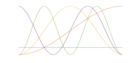
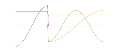
Figure 1: Low frequency eigenmodes of a string (left) and two disconnected pieces of the string (right).

3 Linear graph Laplacian and low frequency eigenmodes of a string

Spectral clustering can be justified intuitively via a well-known identification of the graph Laplacian matrix $L$ with a classical problem of vibrations of a mass-spring system without boundary conditions, with $N$ masses and $M$ springs, where the stiffness of the springs is related to the weights of the graph; see, e.g., [Park20143245]. References [PASTERNAK20146676, Park20143245] consider lateral vibrations, where [PASTERNAK20146676] allows springs with negative stiffness. We prefer the same model, but with transversal vibrations, as in [Demmel99], although the linear eigenvalue problem is the same, for the original graph Laplacian, no matter whether the vibrations are lateral or transversal, under the standard assumptions of infinitesimal displacements from the equilibrium and no damping. The transversal model allows relating the linear mass-spring system to the discrete analog of an ideal string [gould, Fig. 2] and provides the necessary constraints for us to introduce a specific physical realization of inclusions with the negative stiffness by pre-tensing some springs to be repulsive. We start with the simplest example, where the mass-spring system is a discrete string.

3.1 All edges with unit weights

Let $w_{i-1\,i}=w_{i\,i+1}=1$ with all other zero entries, so that the graph Laplacian $L=D-W$ is a tridiagonal matrix

(3.1) $$L=\left(\begin{array}[]{ccccc}1&-1&&&\\ -1&2&-1&&\\ &\ddots&\ddots&\ddots&\\ &&-1&2&-1\\ &&&-1&1\end{array}\right)$$

that has nonzero entries $1$ and $-1$ in the first row, $-1$ and $1$ in the last row, and $[-1\,\;2\,-1]$ in every other row—a standard finite-difference approximation of the negative second derivative of functions with vanishing first derivatives at the end points of the interval. Its eigenvectors are the basis vectors of the discrete cosine transform; see the first five low frequency eigenmodes (the eigenvectors corresponding to the smallest eigenvalues) of $L$ displayed in the left panel in Figure 1. Let us note that these eigenmodes all turn flat at the end points of the interval.

The flatness is attributed to the vanishing first derivatives, which manifests itself in the fact, e.g., that the Laplacian row sums always vanish, including in the first and last rows, corresponding to the “boundary.”

Eigenvectors of matrix (3.1) are well-known in mechanics, as they represent shapes of transversal vibration modes of a discrete analog of a string—a linear system of masses connected with springs. Figure 2 illustrates a system with $N=4$ masses and $M=3$ springs.

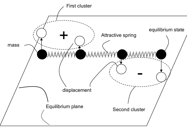
Figure 2: Traditional linear mass-spring system.

The frequencies squared $\omega^{2}$ of the vibration modes $x$ are the eigenvalues $\lambda\geq 0$, e.g.,  [gould, p. 15]. The eigenvectors $x$ of the graph Laplacian can be called eigenmodes because of this mechanical analogy. The smallest eigenvalues $\lambda=\omega^{2}$ correspond to low frequencies $\omega$, explaining the terminology used in the caption in Figure 1. Our system of masses is not attached, thus there is always a trivial eigenmode, where the whole system goes up/down, i.e., the eigenvector $x$ is constant with the zero frequency/eigenvalue $\omega^{2}=\lambda=0$.

If the system consists of $k$ completely separate components, each component can independently move up/down in zero frequency vibration, resulting in total $k+1$ multiplicity of the zero frequency/eigenvalue, where the corresponding eigenvectors are all piecewise constant with discontinuities between the components. Such a system represents a graph consisting of $k$ completely separate sub-graphs and can be used to motivate $k$-way spectral partitioning.

In our case $k=2$, the Fiedler vector is chosen orthogonal to the trivial constant eigenmode, and thus is not only piecewise constant, but also has strictly positive and negative components, determining the two-way spectral partitioning.

Figure 2 shows transversal displacements of the masses from the equilibrium plane for the first nontrivial mode, which is the Fiedler vector, where the two masses on the left side of the system move synchronously up, while the two masses on the right side of the system move synchronously down. This is the same eigenmode as drawn in red color in Figure 1 left panel for a similar linear system with a number of masses large enough to visually appear as a continuous string. Performing the spectral bisection (two-way partitioning) according to the signs of the Fiedler vector, one puts the data points corresponding to the masses in the left half of the mass-spring system into one cluster and those in the right half into the other. The Fiedler vector is not piecewise constant, since the partitioned components are not completely separate.

The amplitudes of the Fiedler vector components are also very important. The amplitude of the component squared after proper scaling can be interpreted as a probability of the corresponding data point to belong to the cluster determined according to the sign of the component. For example, the Fiedler vector in Figure 2 has small absolute values of its components in the middle of the system. With the number of masses increased, the components in the middle of the system approach zero. Perturbations of the graph weights may lead to the sign changes in the small components, putting the corresponding data points into a different cluster.

3.2 A string with a single weak link (small edge weight)

Next, we set a very small value $w_{i\,i+1}=w_{i+1\,i}$ for some index $i$, keeping all other entries of the matrix $W$ the same as before. In terms of clustering, this example represents a situation where there is an intuitively evident bisection with one cluster containing all data points with indexes $1,\ldots,i$ and the other with $i+1,\ldots,N$. In terms of our mass-spring system interpretation, we have a discrete string with one weak link, i.e., one spring with such a small stiffness that makes two pieces of the string nearly disconnected.

Let us check how the low frequency eigenmodes react to such a change. The first five vectors of the corresponding Laplacian are shown in Figure 1, right panel. We observe that all the eigenvectors plotted in Figure 1 are aware of softness (small stiffness) of the spring between the masses with the indexes $i$ and $i+1$. Moreover, their behavior around the soft spring is very specific—they are all flat on both sides of the soft spring!

The presence of the flatness in the low frequency modes of the graph Laplacian $L$ on both sides of the soft spring is easy to explain mathematically. When the value $w_{i\,i+1}=w_{i+1\,i}$ is small relative to other entries, the matrix $L$ becomes nearly block diagonal, with two blocks that approximate the graph Laplacian matrices on sub-strings to the left and right of the soft spring. The low frequency eigenmodes of the graph Laplacian $L$ thus approximate combinations of the low frequency eigenmodes of the graph Laplacians on the sub-intervals.

However, each of the low frequency eigenmodes of the graph Laplacian on the sub-interval is flat on both ends of the sub-interval, as explained above. Combined, it results in the flatness in the low frequency modes of the graph Laplacian $L$ on both sides of the soft spring.

The flatness is also easy to explain in terms of mechanical vibrations. The soft spring between the masses with the indexes $i$ and $i+1$ makes the masses nearly disconnected, so the system can be well approximated by two independent disconnected discrete strings with free boundary conditions, on the left and on the right to the soft spring. Thus, the low frequency vibration modes of the system are visually discontinuous at the soft spring, and nearly flat on both sides of the soft spring.

Can we do better and make the flat ends bend in the opposite directions, making it easier to determine the bisection, e.g., using low-accuracy computations of the eigenvectors? In [knyazev2015edge], where graph-based edge-preserving signal denoising is analyzed, we have suggested to enhance the edges of the signal by introducing negative edge weights in the graph, cf. [1021076]. In the next section, we put a spring which separates the masses by repulsing them and see how the repulsive spring affects the low-frequency vibration modes.

4 Negative weights for spectral clustering

In our mechanical vibration model of a spring-mass system, the masses that are tightly connected have a tendency to move synchronically in low-frequency free vibrations. Analyzing the signs of the components corresponding to different masses of the low-frequency vibration modes determines the clusters.

The mechanical vibration model describes conventional clustering when all the springs are pre-tensed to create attracting forces between the masses, where the mass-spring system is subject to transverse vibrations, i.e., the masses are constrained to move only in a transverse direction, perpendicular to a plane of the mass-spring system. However, one can also pre-tense some of the springs to create repulsive forces between some pairs of masses, as illustrated in Figure 3. For example, the second mass is connected by the attractive spring to the first mass, but by the repulsive spring to the third mass in Figure 3. The repulsion has no effect in the equilibrium, since the masses are constrained to displacements only in the transversal direction, i.e. perpendicular to the equilibrium plane. When the second mass deviates, shown in white circle in Figure 3, from its equilibrium position, shown in back circle in Figure 3, the transversal component of the attractive force from the attractive spring on the left is oriented toward the equilibrium position, while the transversal component of the repulsive force from the repulsive spring on the right is in the opposite direction, resulting in opposite signs in the equation of the balance of the two forces. Since the stiffness is the ratio of the force and the displacement, the attractive spring on the left has effective positive stiffness, but the repulsive spring represents the inclusion with effective negative stiffness, due to the opposite directions of the corresponding forces.

In the context of data clustering formulated as graph partitioning, that corresponds to negative entries in the adjacency matrix. The negative entries in the adjacency matrix are not allowed in conventional spectral graph partitioning. However, the model of mechanical vibrations of the spring-mass system with repulsive springs is still valid, allowing us to extend the conventional approach to the case of negative weights.

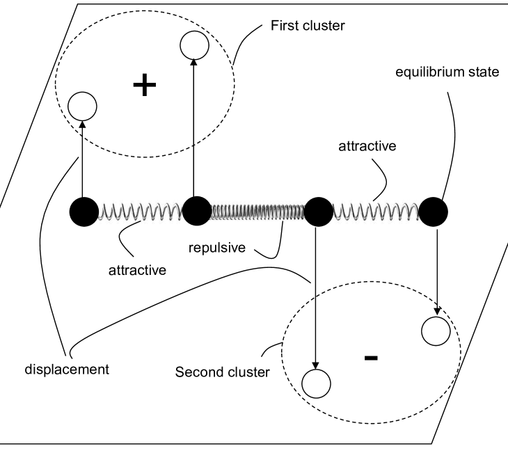
Figure 3: Linear mass-spring system with repulsion.

The masses which are attracted move together in the same direction in low-frequency free vibrations, while the masses which are repulsed have the tendency to move in the opposite direction. Moreover, the eigenmode vibrations of the spring-mass system relate to the corresponding wave equation, where the repulsive phenomenon makes it possible for the time-dependent solutions of the wave equation to exponentially grow in time, if they correspond to negative eigenvalues.

Figure 3 shows the same linear mass-spring system as Figure 2, except that the middle spring is repulsive, bending the shape of the Fiedler vector in the opposite directions on different sides of the repulsive spring. The clusters in Figure 2 and Figure 3 are the same, based on the signs of the Fiedler vectors. However, the data points corresponding to the middle masses being repulsed more clearly belong to different clusters in Figure 3, compared to Figure 2, because the corresponding components in the Fiedler vector are larger by absolute value in Figure 3 vs. Figure 2. Determination of the clusters using the signs of the Fiedler vector is easier for larger components, since they are less likely to be computed with a wrong sign due to data noise or inaccuracy of computations, e.g., small number of iterations.

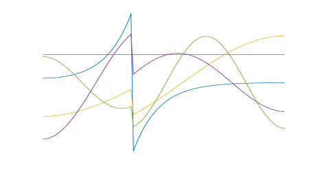
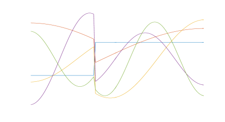
Figure 4: The same eigenmodes, but negative weights, original (left) and signed (right) Laplacians.

Figure 4 left panel displays the five eigenvectors, including the trivial one, for the five smallest eigenvalues of the same tridiagonal graph Laplacian as that corresponding to the right panel in Figure 1 except that the small positive entry of the weights $w_{i\,i+1}=w_{i+1\,i}$ for the same $i$ is substituted by $-0.05$ in Figure 4. Figure 4 right panel displays the five leading eigenvectors of the corresponding signed Laplacian. The left panel of Figure 4 illustrates the predicted phenomenon of the repulsion, in contrast to the right panel. The Fiedler vector of the Laplacian, displayed in blue color in the left panel of Figure 4, is most affected by the repulsion compared to higher frequency vibration modes. This effect gets more pronounced if the negative weight increases by absolute value, as we observe in other tests not shown here.

The Fiedler vector of the signed Laplacian with the negative weight displayed in blue color in the right panel of Figure 4 looks piecewise constant, just the same as the Fiedler vector of the Laplacian with nearly zero weight shown in red color in Figure 1 right panel. We now prove that this is not a coincidence. Let us consider a linear graph corresponding to Laplacian (3.1). We first remove one of the middle edges and define the corresponding graph Laplacian $L_{0}$. Second, we put this edge back but with the negative unit weight $-1$ and define the corresponding signed Laplacian $\bar{L}$. It is easy to verify

(4.2) $$\bar{L}-L_{0}=\left(\begin{array}[]{cccccc}\cdots&\cdots&\cdots&\cdots\\ \cdots&1&1&\cdots\\ \cdots&1&1&\cdots\\ \cdots&\cdots&\cdots&\cdots\end{array}\right),$$

where all dotted entries are zeros.

The Fiedler vector of $L_{0}$ is evidently piece-wise constant with one discontinuity at the missing edge, since the graph Laplacian $L_{0}$ corresponds to the two disconnected discrete string pieces. Let $x_{0}$ denote the Fiedler vector of $L_{0}$ shifted by the vector of ones and scaled so that its components with the opposite sign are simply $+1$ and $-1$, while still $L_{0}x_{0}=0$. We get $(\bar{L}-L_{0})x_{0}=0$ from (4.2), thus, also $\bar{L}x_{0}=0$, i.e., $x_{0}$ is the Fiedler vector of both matrices $\bar{L}$ and $L_{0}$, where in the latter our only negative weight is simply nullified.

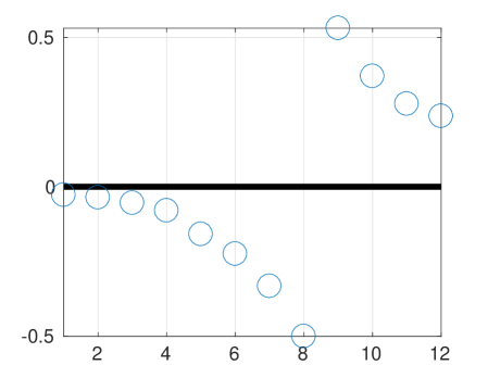
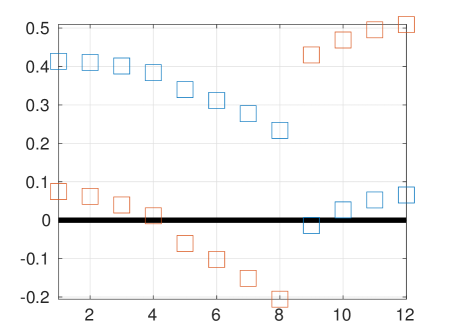
Figure 5: Laplacian eigenmodes, original (left) and signed (right), a “noisy” $12$-mass string with a negative weight at one edge between vertices $8$ and $9$.

5 Comparing the original vs. signed Laplacians

We present a few simple motivating examples, discuss how the original and signed Laplacians are introduced via relaxation of combinatorial optimization, and compare their eigenvectors and gaps in the spectra, computed numerically for these examples.

5.1 Linear graph with noise

We consider another standard linear mass-spring system with $12$ masses and one repulsive spring, $w_{89}=w_{98}=-1/2$ between masses $8$ and $9$, but add to the graph adjacency an extra full random matrix with entries uniformly distributed between $0$ and $10^{-2}$, modelling noise in the data. It turns out that in this example the two smallest eigenvalues of the signed Laplacian form a cluster, making individual eigenvectors unstable with respect to the additive noise, leading to meaningless spectral clustering, if based on the signs on the components of any of the two eigenvectors. Specifically, the exact Laplacian eigenmodes are shown in Figure 5: the original Fiedler (left panel) and both eigenvectors of the signed Laplacian (right panel). The Fiedler vector of the original Laplacian clearly suggests the perfect cut. Neither the first nor the second (giving it a benefit of a doubt) exact eigenvectors of the signed Laplacian result in meaningful clusters, using the signs of the eigenvector components as suggested in [doi:10.1137/1.9781611972801.49].

5.2 “Cobra” graph

Let us consider the mass-spring system in Figure 6, assuming all springs of the same strength, except for the weak spring connecting masses $4$ and $5$, and where one of the springs repulses masses $1$ and $3$. Intuition suggests two alternative partitionings: (a) cutting the weak spring, thus separating the “‘tail” consisting of masses $5$ and $6$, and (b) cutting the repulsive spring and one of the attracting springs, linking mass $3$ or mass $1$ (and $2$) to the rest of the system. Partitioning (a) cuts the weak, but attractive spring; while partitioning (b) cuts one repulsive and one attracting springs of the same absolute strength “canceling” each other influence. If the cost function minimized by the partitioning were the total sum of the removed edges, partitioning (a) would be costlier than (b). Within the variants of the partition (b), the most balanced partitioning is the one separating masses $1$ and $2$ from the rest of the system. Let us now examine the Fiedler vectors of the spectral clustering approaches under our consideration.

The graph corresponding to the mass-spring system in Figure 6, assuming all edges have unit weights, except for the weight $0.2$ of the $(4-5)$ edge, and with $-1$ weight of the $(1-3)$ edge, has the adjacency matrix

(5.3) $$A=\left(\begin{array}[]{cccccc}0&1&-1&0&0&0\\ 1&0&0&1&0&0\\ -1&0&0&1&0&0\\ 0&1&1&0&.2&0\\ 0&0&0&.2&0&1\\ 0&0&0&0&1&0\end{array}\right).$$

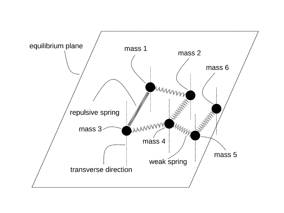
Figure 6: Mass-spring system with repulsive springs.

Let us also consider a graph like the one corresponding to the mass-spring system in Figure 6, but with the repulsive spring eliminated. We nullify the negative weight in the graph adjacency matrix by $A_{0}=\max(A,0)$ and denote the corresponding to $A_{0}$ graph Laplacian matrix by $L_{0}$.

Figure 7 displays the corresponding Fiedler vectors of original $L$ (top left), original with negative weights nullified $L_{0}$ (top right), and both main modes of the signed Laplacian $\bar{L}$ (bottom). The original Laplacian (top left) suggests meaningful clustering of vertices $1$ and $2$ vs. $3$ and $4$. Dropping the negative weight results in cutting the weakly connected tail of the cobra, see Figure 7 top right. The first eigenvector of the signed Laplacian in Figure 7 bottom right appears meaningless for clustering, even though it is far from looking as a constant. The second eigenvector of the signed Laplacian in Figure 7 bottom left suggests cutting off vertex $3$ from $1$ and $2$, which is not well balanced.

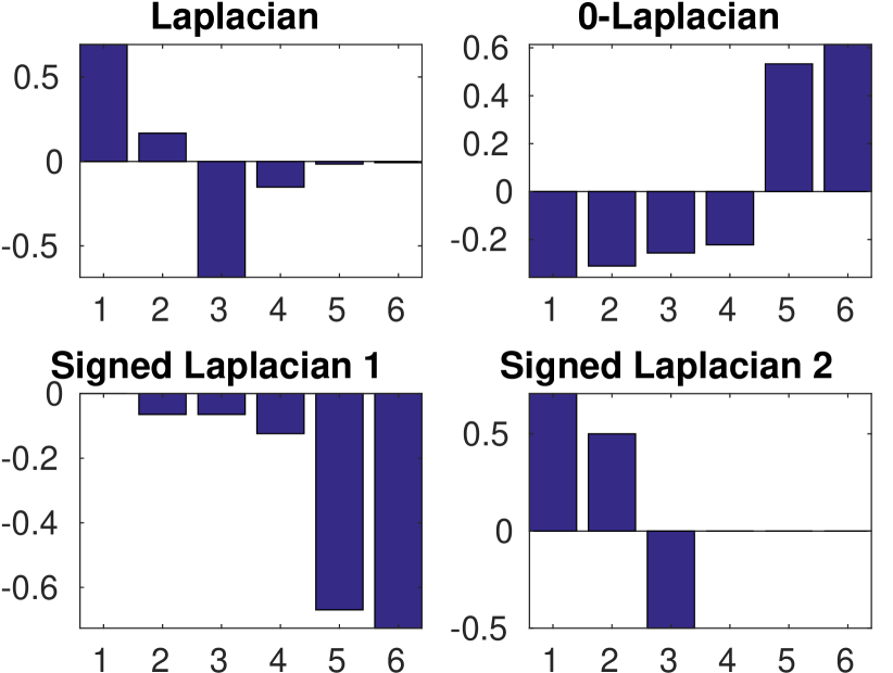
Figure 7: Laplacian eigenvectors: the original $L$ (top left), the original with negative weights nullified $L_{0}$ (top right), and the signed Laplacian $\bar{L}$ first (bottom right) and second (bottom left) eigenvectors, for a $6$-mass string with a negative weight at one edge between vertices $1$ and $3$.

5.3 “Dumbbell” graph