trbstyle Sokolov, Larson, Munson, Auld, and Karbowski0   table figure

Platoon formation maximization through centralized routing and departure time coordination

Abstract

Platooning allows vehicles to travel with small intervehicle distance in a coordinated fashion thanks to vehicle-to-vehicle connectivity. When applied at a larger scale, platooning will create significant opportunities for energy savings due to reduced aerodynamic drag, as well as increased road capacity and congestion reduction resulting from shorter vehicle headways. However, these potential savings are maximized if platooning-capable vehicles spend most of their travel time within platoons. Ad hoc platoon formation may not ensure a high rate of platoon driving. In this paper we consider the problem of central coordination of platooning-capable vehicles. By coordinating their routes and departure times, we can maximize the fuel savings afforded by platooning vehicles. The resulting problem is a combinatorial optimization problem that considers the platoon coordination and vehicle routing problems simultaneously. We demonstrate our methodology by evaluating the benefits of a coordinated solution and comparing it with the uncoordinated case when platoons form only in an ad hoc manner. We compare the coordinated and uncoordinated scenarios on a grid network with different assumptions about demand and the time vehicles are willing to wait.

1. Introduction

Platoons are composed of multiple vehicles communicating with each other and whose movements are automatically controlled. A vehicle in a platoon knows with good accuracy the gap with the preceding vehicle and with the leading vehicle thanks to sensors and radio communication. Each vehicle can thus adjust its speed with full awareness of the state of the preceding and lead vehicles, allowing it to safely maintain a shorter gap between vehicles (1). Further, researchers have shown (2) that drivers are comfortable with a following time-gap as low as 0.6 seconds.

Platooning also provides the prospect of reducing the massive waste incurred by traffic congestion. A 2011 study shows urban road congestion annually costing $121 billion dollars based on 5.5 billion man-hours and 2.9 billion gallons of wasted fuel (3); and increasing urban population will likely exacerbate these effects. Platooning can help alleviate congestion by addressing the highly inefficient use of road space by human drivers: congestion occurs when vehicles occupy only 18% of the road for a typical highway with 2,200 vehicles per hour capacity (4). Vehicles equipped with Cooperative Adaptive Cruise Control (CACC) (which allows for a simpler form of platooning) have been shown to improve traffic flow and more efficiently use road space (1, 2). The impact of CACC vehicles at different market penetration rates on a regional scale have been studied via simulations in (5, 6), and their impact on throughput at intersections in an urban road system was simulated in (7). The simulation studies show that CACC enables shorter following gaps and increases road capacity from the typical 2,200 vehicles per hour to almost 4,000 vehicles per hour at 100% market penetration.

Platooning vehicles also use less fuel because trailing vehicles experience a reduced aerodynamic drag. A study was conducted in (8) involving three trucks driving 80 km/h with 10 m intervehicle gaps, where control algorithms for lateral movement relied on radar measurements and vehicle-to-vehicle communication. Analysis of their field data shows a 14% decrease in fuel use. Under similar speeds (60 and 80 km/h) and headway conditions (0.3 to 0.45 seconds) a platoon of two trucks is studied in (9). The trucks were connected through an electronic system comprising a vehicle-to-vehicle controller, a tow bar controller, and an image-processing unit. Overall, the reduction in fuel consumption ranged from 15% to 21% at 80 km/h and 10% to 17% at 60 km/h. In (10), the authors studied fuel consumption of two trucks linked via an electronic control system and report 8–11% fuel savings. In (11), the authors tested speed control algorithms for following vehicles that use information about the road ahead sensed by the lead vehicle. They showed a 5–8% improvement in fuel efficiency. Computational fluid dynamics simulations confirm field studies and show that an optimal headway distance that minimizes drag forces is 6–8 meters; this leads to fuel savings of 7–15% (12). Studies for light-duty vehicles show similar savings (13, 14, 15, 6).

In this paper we focus on minimizing the collective fuel use of a group of vehicles by coordinating their departure time and routing, and we then measure the fraction of total miles traveled in a platoon for a given set of trips. An optimal routing is computed by jointly computing vehicle routes and departure times. Routing existing platoons in a network has been studied and solved by a number of authors using discretized optimal control (16, 17, 18), dynamic programming (19, 20), and graph-based algorithms (21). These methods are applied to relatively small networks: those with 3–10 nodes and 6–34 arcs. In contrast to our coordinated model, the platoons in these models are not allowed to merge with other vehicles and consequently save additional fuel; they consider only the optimal routing after the vehicles have been grouped into platoons.

The goal of this paper is to analyze the potential improvements that can be achieved by strategic coordinated platooning. The coordination assumes that drivers are willing to delay their departures in order to be able to travel in a platoon. We analyze different levels of willingness to wait and how such waiting affects the optimal fuel savings. We present a coordinated platooning optimization model and evaluate the impact of optimal platoon routing by comparing it with an ad hoc platoon formation strategy. The optimization model attempts to minimize the collective fuel use by routing vehicles through the network while determining when platoons should form or dissolve. An explicit mixed-integer programming model in the GAMS modeling language (22) and example problem data are available at

http://www.mcs.anl.gov/~jlarson/Platooning.

The paper is organized as follows. Section 2 describes the transportation system model used for opportunistic platooning simulations. Section 3 presents our coordinated platooning optimization model. Section 4 provides numerical results for a metropolitan road network and compares coordinated and uncoordinated platooning with different assumptions on travel demand and the willingness of drivers to delay their departures. We conclude with a discussion in Section 5.

2. Opportunistic Platooning Simulations

We use POLARIS, a transportation system simulator (23), to simulate ad hoc (or opportunistic) platooning. POLARIS is a fully integrated, agent-based simulation of both vehicles and traffic operations. The simulation integrates travel demand, network simulation, and network operation models. At the center of POLARIS is a person-agent that represents travelers in the system and their activity and travel behavior. The agents plan and schedule their daily activities according to a variety of behavior rules and choice processes and then travel through the network to meet their individual objectives. When traveling from one location to another according to the behavioral objectives, the agents choose routes through the network that minimize a personal cost function. The agents then operate in an environment, represented by the transportation network model, that handles movements through the system governed by the route choice. The route can be replanned by the agent in response to network conditions, new information, and direct system control.

The POLARIS simulator uses a variant of the Lighthill-Whitham-Richards (LWR) (24, 25) traffic flow model, which is a combination of a conservation law defined via a partial differential equation and a flow-density relation called the fundamental diagram. The nonlinear first-order partial differential equation describes the aggregate behavior of drivers. The model explicitly represents the dynamics of the primary variable of interest, traffic density, which is a macroscopic characteristic of traffic flow and the key control variable in transportation system management strategies. Traffic density is defined as a number of vehicles per unit of length. The model is well studied and is used in many transportation applications (26, 27, 28).

The partial differential equation underlying POLARIS is solved by using Newell’s simplified kinematic waves traffic flow discretization scheme (29). This is a link-based solution method and has been recently recognized as an efficient and effective method for large-scale networks (30) and dynamic traffic assignment formulations (31). A notable implementation of this model is in an open-source dynamic traffic assignment tool DTALite (32). This tool is used as the traffic simulation model agent in the POLARIS framework.

The traffic simulation model includes a set of traffic simulation agents for intersections, links, and traffic controls. Given a set of travelers with route decisions and the network’s traffic operation and control strategies, the network model simulates traffic operations to provide capacities and driving rules on links as well as drivers’ turn movements at intersections. With these capacity and driving rule constraints, link and intersection agents simulate the traffic flows using cumulative departures and arrivals as decision variables based on Newell’s model. This model then determines the network performance for the route and demand models in the integrated framework. The traffic simulation model agents also produce a set of measures of effectiveness such as their average speed, density, and flow rate, as well as individual vehicle trajectories. The exact solution developed by Newell (33) is given by

$$\begin{split}T(x,n)=\max\left(T(x_{u},n)+\frac{x-x_{u}}{u},\right.\left.~{}T\left(x_{d},n-\rho_{jam}(x_{d}-x)\right)+\frac{x_{d}-x}{w}\right),\end{split}$$

where $T(x,n)$ is the time when vehicle $n$ crosses location $x$ on the link, $w$ is the shock wave propagation speed, $u$ is the free-flow speed, and $\rho_{jam}$ is the jam density of the road segment. Note that $w$, $u$, and $\rho_{jam}$ are the parameters of the fundamental diagram. An event-based simulation scheme is implemented by using POLARIS’s discrete event engine, and the traffic flow simulator is integrated with other transportation simulation components.

We modified the POLARIS traffic flow model to account for opportunistic platoon formation. In our study we did not simulate changes in travel demand as a result of automation and assumed a fixed demand specified in an input trip table. Each vehicle in the trip table is labeled as either a platoon-capable vehicle or a regular vehicle. When simulating mixed traffic with platooning and regular vehicles, vehicles of both type will propagate along a link according to the LWR model. However, the fundamental diagram of a road link is dynamically adjusted to account for the presence of automated vehicles. Since the LWR model preserves the first-in-first-out property of the traffic flow, we assume that two platoon-capable vehicles entering the same road segment one after another will platoon on this link. We dynamically adjust the capacity of the road segment as a function of the number of vehicles platooning on this road segment. The capacity adjustment factors used were derived in (5, 6).

3. Optimization Model

The set of POLARIS-simulated trips is then sent to the external optimization model in order to find optimal wait times and routes for maximizing the time spent in a platoon. A complete description of the optimization model can be found in (34). We briefly describe the model variables and objective function from the optimization model. Given a collection of vehicles and a road network described by a set of nodes and edges, our model requires (1) the (fixed) cost to traverse any edge in the network, (2) the origin and destination nodes for each vehicle, (3) the time each vehicle arrives in the network, and (4) the time each vehicle must be at its destination. We assume that the times are feasible, that is, that each vehicle’s destination time is at least their origin time plus the shortest path time from its origin to its destination. For our simulations, we assume vehicles are willing to wait a short period of time at their origin nodes provided they can save fuel by platooning, but we do not allow vehicles to wait at intermediate nodes.

Given a problem instance defined by these parameters, the optimization model chooses routes and departure times for each vehicle so that the collective fuel use is minimized while ensuring that each vehicle reaches its destination on time. If $n$ vehicles travel on the same road segment at the same time, $n-1$ use 10% less fuel than the remaining vehicle (which is assumed to be leading the platoon).

Our objective is to minimize the overall fuel consumed. We use a simple assumption that the amount of fuel consumed by a vehicle while traversing an edge $(i,j)$ is constant, and we denote it by $C_{i,j}$. We denote the delay in departure time of vehicle $v$ at its origin by $t_{v}$, the fraction of fuel saved by platooning by $\eta$, and the cost of waiting by each vehicle by $\epsilon_{v}$. For our study, $C_{i,j}=1$ for all edges in the grid and $\eta=0.1$. If the decision variable $f_{v,i,j}=1$ when vehicle $v$ takes $(i,j)$ and $q_{v,w,i,j}=1$ if vehicle $v$ follows vehicle $w$ on $(i,j)$, then the objective function is

$$\sum_{v,i,j}C_{i,j}\left(f_{v,i,j}-\eta\sum_{w}q_{v,w,i,j}\right)+\epsilon_{v}t_{v}.$$ (1)

In our current study we focus on the maximal possible savings and set $\epsilon_{v}=0$. For fleet managers coordinating the routes of many vehicles, $\epsilon_{v}$ should be the cost per unit time for a stationary vehicle: the drivers’ wages plus any idling costs. Such a straightforward calculation is less obvious for private drivers. Also, individuals may need additional incentives in order to be willing to add even a short period of time to their commutes in order to reduce their fuel use by 10%.

Note that a naive implementation of the prescribed model will quickly become computationally intractable because of, for example, generating binary variables $q$ for all pairs of vehicles and all edges in the network. A more systematic approach, used in the available code and discussed in depth in (34), is to generate variables only when necessary. A vehicle will not travel more that $\frac{1}{1-\eta}$ times its shortest-path route between its origin and destination (34, Lemma 2.2); therefore, most $f_{v,i,j}$ can be removed for most edges in a real-world network. Similarly, $q_{v,w,i,j}$ need exist only if vehicles $v$ and $w$ can possibly traverse edge $(i,j)$ simultaneously given their origin/destination times. Such considerations dramatically reduce the model size.

Naturally, this model requires a collection of constraints. Any vehicle that enters a nondestination node must exit it. If vehicles are platooning on an edge, the times they enter the edge must be equal. A vehicle cannot enter another edge until it has traversed its current edge. For a thorough discussion of the model and constraints, see (34).

4. Case Study

To test the effects of coordinated and uncoordinated platooning, we performed experiments on the $10\times 10$ grid shown in Figure 1, in which each link has a length of 1 km. Even though the grid model network used in this study appears simple, finding the optimal solution on such grid network is more challenging than on a real highway network since many different routes of the same length exist between most pairs of origin/destination nodes. The number of shortest paths between $(0,0)$ and $(m,n)$ in a grid is ${m+n\choose n}$, whereas on a highway network there are usually a very small number of valid alternative routes between an origin and a destination (usually not more than two). In this case study we assume no congestion on the network, and the cost of traversing a road link is assumed to be proportional to free-flow travel time on this link.

FIGURE 1 : Network under consideration: a $10\times 10$ grid

Origins and destinations are randomly generated for 50 vehicles. The trip length distribution is shown in Figure 2; its mean is 7 km. We make the simplifying assumption that all 50 vehicles can be rerouted and controlled and that their coordination does not affect link travel times. This will not hold as more vehicles are routed, but it is a valid assumption when small percentages of vehicles are under control.

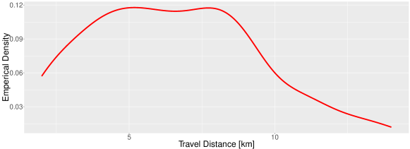
FIGURE 2 : Distribution of trip length

The departure times $T^{O}_{v}$ for each vehicle $v$ are randomly drawn from a truncated normal distribution with support of $[0,100]$, mean 50, and 6 different standard deviations. The departure time distributions are shown in Figure 3. Each vehicle must arrive at its destination at time $T^{D}_{v}$, set to

$$T^{v}_{D}=T^{v}_{O}+T_{O_{v},D_{v}}+p,$$ (2)

where $T_{O_{v},D_{v}}$ is the minimum time between the vehicle’s origin and destination and $p$ is some pause time. We assume that trailing vehicles in a platoon use 10% less fuel than do vehicles leading a platoon or traveling alone on a given edge.

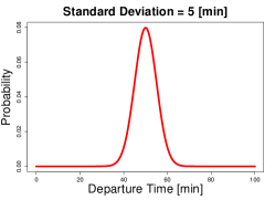
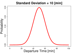
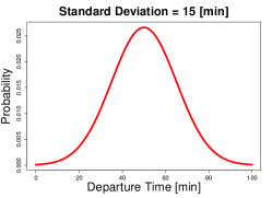
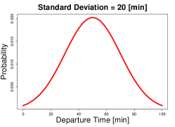
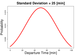
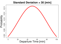
FIGURE 3 : Six scenarios for departure time distribution

One of the most important parameters for maximizing driving in platoons is $p$, the upper bound on the amount of time vehicles are willing to wait. Naturally, the longer vehicles are willing to wait, the more platooning possibilities exist, and therefore platooning can occur. If the pause time $p$ in (2) is zero, then every vehicle must travel from its origin to its destination along its shortest path and can participate only in ad hoc platoons. This scenario corresponds to the uncoordinated platooning case. If $p>0$, a vehicle can wait to lead/follow another vehicle, thereby decreasing the collective fuel use. In our experiments, increasing $p$ past a certain value provides no additional savings. We simulated our case study with five maximum possible wait times: $p\in\{0,10,20,30,40\}$. We ran Gurobi for five minutes on each GAMS model of each problem instance.

For our case study we use wait time and the vehicle-miles-traveled (VMT) ratio to estimate the efficiency of the optimal routing when compared with opportunistic platooning. The VMT ratio is the ratio of miles driven in a platoon to the total miles driven by a vehicle.

$$\mathrm{VMT~{}ratio}=\dfrac{\mathrm{Platoon~{}VMT}}{\mathrm{Total~{}VMT}}$$

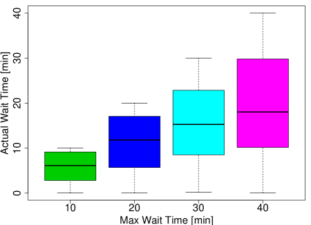
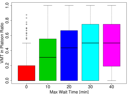
(a) Actual wait times	(b) Ratio of distance driven in platoon

FIGURE 4 : Box plots comparing the impact of coordinated platooning for different assumptions on maximum allowed wait time. Panel (a) compares actual wait times experienced by drivers. Panel (b) compares the ratio of distance driven in a platoon.

Figure 4 shows a summary of the simulated results for the case study. We compare results for different assumptions about the maximum wait time. This parameter controls the amount of time by which each driver is willing to delay his/her departure time, with zero corresponding to the opportunistic platooning scenario; that is, drivers depart at the originally intended time and platoon only in an ad hoc fashion. For each scenario we calculate two metrics: the ratio of distance driven in a platoon and the average wait time. Naturally, the average wait time is less than maximum wait time and is zero for opportunistic platooning scenario, so it is not shown on Figure 4(a).

The average platoon distance ratio for opportunistic platooning is 0.12. On the other hand, for coordinated platooning when we set the maximum wait time to 10, the average distance-in-platoon ratio is nearly tripled to 0.32. Note that the average wait time for this scenario is 5 minutes, which is well below the upper bound of 10 minutes.

The largest gain in the platoon distance ratio is when we switch from the opportunistic platooning scenario (maximum wait time = 0) to the optimal platooning with a maximum wait time of 10 minutes. For a maximum wait time larger than 10 minutes we do not see significant improvement in the ratio.

However, the benefits of platooning (i.e., energy savings) must be traded with the extra wait time required under strategic routing of automated vehicles scenario. Making assumptions about the mean fuel consumption (gallon/miles) and value of time ($/hour), one can calculate savings associated with the strategic routing by

$$\mbox{Savings}=\mbox{VMT in Platoon}\times\eta\times\mbox{Fuel Consumption}\times\mbox{Fuel Cost}-\mbox{Wait}\times\mbox{Value of Time}.$$

Here $\eta$ is the ratio of fuel saved while driving in a platoon. Assuming $\eta=0.1$, $\mbox{Fuel Consumption}=0.04$ gallons/miles, (equivalent to 25 mpg), $\mbox{Value of Time}=30$ $/hour, and $\mbox{Fuel Cost}=3$ $/gallon we calculate the distribution of the savings associated with the centralized routing strategy. Figure 5 shows the results for different assumptions about maximum wait time and departure time distributions.

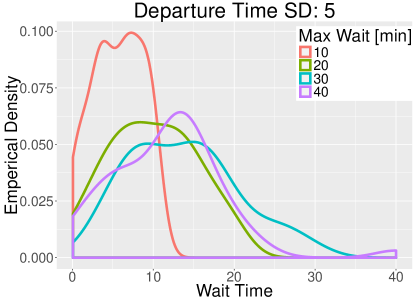
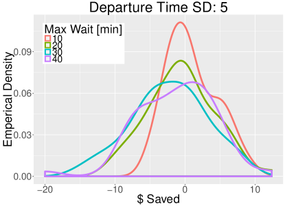
(a) Wait Time Distribution	(b) Dollar Savings

FIGURE 5 : Distribution of departure time delays calculated by optimization algorithm and economic savings for the system users

We can see from Figure 5(a) that the wait time distribution does not change for scenarios with wait times greater than 10, hence there exists some threshold beyond which an increase in the wait time does not bring benefits. On the other hand, when we contrast the wait time with the net economic benefit shown in Figure 5(b), we see that under our assumptions, it is negative for all of the users. Thus, for such a system to be viable, additional benefits should be associated with centralized routing strategy. Examples of such benefits might include saved travel times as a result of reduced congestion or incentives for CACC drivers such as reduced tolls or access to dedicated lanes. Assessing the impact of centralized routing strategies on the systemwide congestion levels is the direction of our future research.

As part of the analysis framework we developed a web-based animation of the optimization results for the grid network. Snapshots of the animated visualization are shown on Figure 6.

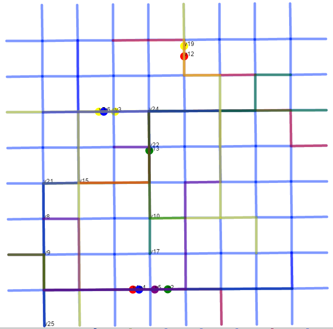
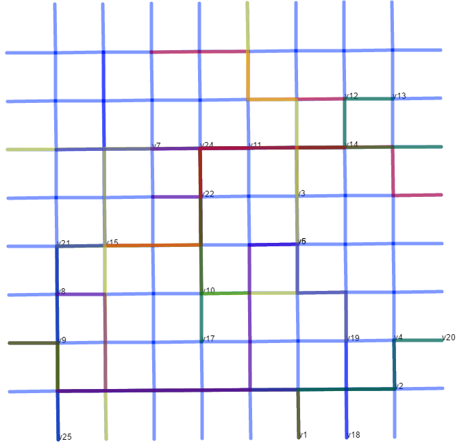
FIGURE 6 : Snapshot for optimal platoons

Animation of the solutions on an instance of the optimization problem with 25 vehicles is available at http://polaris.es.anl.gov/cav_map_notiles/.

5. Discussion

In this paper we demonstrated a method of coordinating platoon formation in which vehicles routes and departure times are strategically chosen by a centralized authority. We showed that at reasonable waiting times, one can substantially increase the distances vehicles travel in a platoon when a coordinated approach is used. To our knowledge this is one of the first papers that presents a relatively large-scale case study of coordinated platooning and compares such an approach with the uncoordinated case. We used Gurobi to solve GAMS models to find optimal routes and departure times. We used the transportation system modeling framework POLARIS to simulate the uncoordinated platooning case. POLARIS can simulate large-scale transportation systems with millions of trips in a matter of hours. Thus, it can be used to analyze the impacts of opportunistic platooning for large-scale models. However, the underlying optimization problem for coordinated platooning is the combinatorial optimization that currently scales poorly with the number of vehicles. Certain assumptions and modeling tricks have allowed us to solve problem instances with 50 vehicles for a fairly complicated network.

Current research includes considering possible heuristic rules in order to improve the solution times of the optimization model on larger problems, with the goal of solving instances with thousands of vehicles. POLARIS is also being adjusted to model a mix of platooning and nonplatooning vehicles. Provided that vehicles are traveling at free-flow speeds, the simulation setup and optimization model are still accurate. The congested network case is considerably more difficult to address. We are exploring using the optimization model as an open-loop controller to feed into POLARIS. When the network is congested, care is being taken to ensure that the routes produced by the optimization model are feasible and converge to a stable routing. We are also working to relax the optimization model assumption that platooning vehicles travel at free-flow speeds in order to accurately analyze congested networks. Moreover, we are analyzing fuel savings using the high-fidelity vehicle energy model AUTONOMIE (35, 36) in order to better understand the impacts of coordinated platooning. Considering the impact of traffic lights on platoon formation and energy savings (7) is another direction for future research.

The submitted manuscript has been created by UChicago Argonne, LLC, Operator of Argonne National Laboratory (“Argonne”). Argonne, a U.S. Department of Energy Office of Science laboratory, is operated under Contract No. DE-AC02-06CH11357. The U.S. Government retains for itself, and others acting on its behalf, a paid-up, nonexclusive, irrevocable worldwide license in said article to reproduce, prepare derivative works, distribute copies to the public, and perform publicly and display publicly, by or on behalf of the Government.

References

- Lu and Shladover (2011) Lu, X.-Y. and S. E. Shladover, Automated truck platoon control. California PATH Research Report UCB-ITS-PRR-2011-13, 2011.
- Nowakowski et al. (2010) Nowakowski, C., J. O’Connell, S. E. Shladover, and D. Cody, Cooperative adaptive cruise control: Driver acceptance of following gap settings less than one second. In Proceedings of the Human Factors and Ergonomics Society Annual Meeting, SAGE Publications, 2010, Vol. 54, pp. 2033–2037.
- Schrank et al. (2012) Schrank, D., B. Eisele, and T. Lomax, TTI’s 2012 urban mobility report. Texas A&M Transportation Institute, 2012.
- Manual et al. (2000) Manual, H. C. et al., Transportation research board. National Research Council, Washington, DC, Vol. 113, 2000.
- Vander Werf et al. (2002) Vander Werf, J., S. Shladover, M. Miller, and N. Kourjanskaia, Effects of adaptive cruise control systems on highway traffic flow capacity. Transportation Research Record: Journal of the Transportation Research Board, Vol. 1800, 2002, pp. 78–84.
- Shladover et al. (2012) Shladover, S., D. Su, and X.-Y. Lu, Impacts of cooperative adaptive cruise control on freeway traffic flow. Transportation Research Record: Journal of the Transportation Research Board, Vol. 2324, 2012, pp. 63–70.
- Lioris et al. (2016) Lioris, J., R. Pedarsani, F. Y. Tascikaraoglu, and P. Varaiya, Doubling throughput in urban roads by platooning. IFAC-PapersOnLine, Vol. 49, No. 3, 2016, pp. 49–54, 14th IFAC Symposium on Control in Transportation Systems.
- Tsugawa (2013) Tsugawa, S., An overview on an automated truck platoon within the energy ITS project. In Advances in Automotive Control, 2013, Vol. 7, pp. 41–46.
- Bonnet and Fritz (2000) Bonnet, C. and H. Fritz, Fuel consumption reduction in a platoon: Experimental results with two electronically coupled trucks at close spacing. Intelligent Vehicle Technology - SP-1558, 2000.
- Browand et al. (2004) Browand, F., J. McArthur, and C. Radovich, Fuel saving achieved in the field test of two tandem trucks. California PATH Research Report UCB-ITS-PRR-2004-20, 2004.
- Alam et al. (2010) Alam, A. A., A. Gattami, and K. H. Johansson, An experimental study on the fuel reduction potential of heavy duty vehicle platooning. In Proceedings of the 13th International IEEE Conference on Intelligent Transportation Systems, IEEE, 2010, pp. 306–311.
- Dávila (2013) Dávila, A., SARTRE report on fuel consumption. Technical Report for European Commission under the Framework 7 Programme Project 233683 Deliverable 4.3., 2013.
- Shida and Nemoto (2009) Shida, M. and Y. Nemoto, Development of a small-distance vehicle platooning system. In 16th ITS World Congress and Exhibition on Intelligent Transport Systems and Services, 2009.
- Shida et al. (2010) Shida, M., T. Doi, Y. Nemoto, and K. Tadakuma, A short-distance vehicle platooning system (second report): Evaluation of fuel savings by the developed cooperative control. In Proceedings of the 10th International Symposium on Advanced Vehicle Control, 2010, pp. 719–723.
- Eben Li et al. (2013) Eben Li, S., K. Li, and J. Wang, Economy-oriented vehicle adaptive cruise control with coordinating multiple objectives function. Vehicle System Dynamics, Vol. 51, No. 1, 2013, pp. 1–17.
- Baskar et al. (2009a) Baskar, L. D., B. De Schutter, and H. Hellendoorn, Optimal routing for intelligent vehicle highway systems using mixed integer linear programming. In Proceedings of the 12th IFAC Symposium on Control in Transportation Systems (A. Chassiakos, ed.), Elsevier, 2009a, pp. 569–575.
- Baskar et al. (2013) Baskar, L. D., B. De Schutter, and H. Hellendoorn, Optimal routing for automated highway systems. Transportation Research Part C: Emerging Technologies, Vol. 30, 2013, pp. 1–22.
- Baskar et al. (2009b) Baskar, L. D., B. De Schutter, and J. Hellendoorn, Optimal routing for intelligent vehicle highway systems using a macroscopic traffic flow model. In Proceedings of the 12th International IEEE Conference on Intelligent Transportation Systems (M. Barth, ed.), IEEE, 2009b, pp. 1–6.
- Garcia et al. (1995) Garcia, A., R. L. Smith, and R. Sengupta, Dynamic programming heuristic for system optimal routing in dynamic traffic networks. Technical Report 95-22, 1995.
- Valdés et al. (2012) Valdés, F., R. Iglesias, F. Espinosa, and M. A. Rodríguez, An efficient algorithm for optimal routing applied to convoy merging manoeuvres in urban environments. Applied Intelligence, Vol. 37, No. 2, 2012, pp. 267–279.
- van Doremalen (2015) van Doremalen, K. P., Platoon coordination and routing. Master’s Internship Report, Eindhoven University of Technology, 2015.
- GAMS Development Corporation (2013) GAMS Development Corporation, General Algebraic Modeling System (GAMS) Release 24.2.1, 2013.
- Auld et al. (2016a) Auld, J., M. Hope, H. Ley, V. Sokolov, B. Xu, and K. Zhang, POLARIS: Agent-based modeling framework development and implementation for integrated travel demand and network and operations simulations. Transportation Research Part C: Emerging Technologies, Vol. 64, 2016a, pp. 101–116.
- Lighthill and Whitham (1955) Lighthill, M. J. and G. B. Whitham, On kinematic waves II: A theory of traffic flow on long crowded roads. The Royal Society, 1955, Vol. 229, pp. 317–345.
- Richards (1956) Richards, P. I., Shock waves on the highway. Operations Research, Vol. 4, No. 1, 1956, pp. 42–51.
- Lebacque (2005) Lebacque, J.-P., First-order macroscopic traffic flow models: Intersection modeling, network modeling. In Transportation and Traffic Theory. Flow, Dynamics and Human Interaction. 16th International Symposium on Transportation and Traffic Theory, 2005.
- Lebacque (1996) Lebacque, J.-P., The Godunov scheme and what it means for first order traffic flow models. In Internaional Symposium on Transportation and Traffic Theory, 1996, pp. 647–677.
- Hoogendoorn and Bovy (2001) Hoogendoorn, S. P. and P. H. Bovy, State-of-the-art of vehicular traffic flow modelling. Proceedings of the Institution of Mechanical Engineers, Part I: Journal of Systems and Control Engineering, Vol. 215, No. 4, 2001, pp. 283–303.
- Newell (1993) Newell, G., A simplified theory of kinematic waves in highway traffic, Part I: General theory. Transportation Research Part B: Methodological, Vol. 27, No. 4, 1993, pp. 281 – 287.
- Lu et al. (2013) Lu, C.-C., X. Zhou, and K. Zhang, Dynamic origin–destination demand flow estimation under congested traffic conditions. Transportation Research Part C: Emerging Technologies, Vol. 34, 2013, pp. 16–37.
- Zhang et al. (2013) Zhang, K., X. Zhou, and C. Lu, Novel integer program formulation for dynamic traffic assignment problem. In Proceedings of the 92nd Annual Meeting of the Transportation Research Board (DVD), 2013.
- Zhou and Taylor (2014) Zhou, X. and J. Taylor, DTALite: A queue-based mesoscopic traffic simulator for fast model evaluation and calibration. Cogent Engineering, Vol. 1, No. 1, 2014, p. 961345.
- Newell (1999) Newell, G., A simplified car-following theory: a lower order model. Research report, University of California, Berkeley. Institute of Transportation Studies, 1999.
- Larson et al. (2016) Larson, J., T. Munson, and V. Sokolov, Coordinated Platoon Routing in a Metropolitan Network. In Proceedings of the SIAM Workshop on Combinatorial Scientific Computing (to appear), SIAM, 2016.
- Argonne National Laboratory (2016) Argonne National Laboratory, AUTONOMIE. http://www.autonomie.net/, accessed 10/31/2016.
- Auld et al. (2016b) Auld, J., D. Karbowski, V. Sokolov, and N. Kim, A disaggregate model system for assessing the energy impact of transportation at the regional level. In Transportation Research Board 95th Annual Meeting, 2016b, 16-2416.