The lognormal-like statistics of a stochastic squeeze process

Abstract

We analyze the full statistics of a stochastic squeeze process. The model’s two parameters are the bare stretching rate $w$, and the angular diffusion coefficient $D$. We carry out an exact analysis to determine the drift and the diffusion coefficient of $\log(r)$, where $r$ is the radial coordinate. The results go beyond the heuristic lognormal description that is implied by the central limit theorem. Contrary to the common “Quantum Zeno” approximation, the radial diffusion is not simply $D_{r}=(1/8)w^{2}/D$, but has a non-monotonic dependence on $w/D$. Furthermore, the calculation of the radial moments is dominated by the far non-Gaussian tails of the $\log(r)$ distribution.

I Introduction

In this paper we analyze the full statistics of a physically-motivated stochastic squeeze process that is described by the Langevin (Stratonovich) equation

$$\dot{x}\ = \ \ \ wx\ -\ \omega(t)y$$

$$\dot{y}\ = \ -wy\ +\ \omega(t)x$$ (1)

where the rotation frequency $\omega(t)$ is a zero mean white noise with fluctuations:

$${}\left\langle\omega(t^{\prime})\omega(t^{\prime\prime})\right\rangle\ =\ 2D\delta(t^{\prime}-t^{\prime\prime})$$ (2)

Accordingly the model has two parameters: the angular diffusion coefficient $D$ of the polar phase, and the bare stretching rate $w$ of the radial coordinate ${r=\sqrt{x^{2}+y^{2}}}$. In a physical context the noise arises due to the interaction with environmental degrees of freedom, typically modeled as an harmonic bath of “phonons”. Hence we can assume for it a Gaussian-like distribution with bounded moments. The white noise assumption means that the correlation time is very short, hence the Stratonovich interpretation of Eq.​​ (1) is in order, as argued, for example, by Van Kampen VanKampen1981 .

The squeeze operation is of interest in many fields of science and engineering, but our main motivation originates from the quantum mechanical arena, where it is known as parametric amplification. In particular it describes the dynamics of a Bosonic Josephson Junction (BJJ) given that all the particles are initially condensed in the upper orbital. Such preparation is unstable Chuchem10 ; chapman , but it can be stabilized by introducing frequent measurements or by introducing noise. This is the so-called “quantum Zeno effect” (QZE) QZE1 ; QZE3 ; QZE4 ; Kofman2 ; Gordon1 . The manifestation of the QZE in the BJJ context has been first considered in QZESQ1 ; QZESQ2 , and later in KhripkovVardiCohen2012 .

The main idea of the QZE is usually explained as follows: The very short-time decay of an initial preparation due to a constant perturbation is described by the survival probability ${\mathcal{P}(t)=1-(vt)^{2}}$, where $v$ is determined by pertinent couplings to the other eigenstates; Dividing the evolution into $\tau$-steps, and assuming a projective measurement at the end of each step one obtains

$$\mathcal{P}(t) \approx \left[\mathcal{P}(\tau)\right]^{t/\tau}\approx\left[1-(v\tau)^{2}\right]^{t/\tau}\approx\exp\left[-(v^{2}\tau)t\right]$$

The common phrasing is that frequent measurements (small $\tau$) slow down the decay process due to repeated “collapse” of the wavefunction. Optionally one considers a system that is coupled to the environment. Such interaction is formally similar to a continuous measurement process, that is characterized by a dephasing time $\tau$. In the latter case the phrasing is that the introduction of “noise” leads to the slow-down of the decay process. Contrary to simple minded intuition, stronger noise leads to slower decay.

At this point one might get the impression that the QZE is a novel “quantum” effect, that has to do with mysterious collapses, and that such effect is not expected to arise in a “classical” reality. Such conclusion is in fact wrong: whenever the the system of interest has a meaningful classical limit, the same Zeno effect arises also in the classical analysis. This point has been emphasized by Ref.KhripkovVardiCohen2012 in the context of the BJJ. It has been realized that the QZE is the outcome of the classical dynamics that is is generated by Eq.​​ (1), where the ${(x,y)}$ are local canonical conjugate coordinates in the vicinity of an hyperbolic (unstable) fixed-point in phase space. The essence of the QZE in this context is the observation that the introduction of the noise via the phase-variable leads to slow-down of the radial spreading. For strong noise (large $D$ in Eq.​​ (2)), the radial spreading due to $w$ is inhibited. Using quantum terminology this translates to suppression of the decoherence process.

From pedagogical point of view it is useful to note that the dynamics of the BJJ is formally similar to that of a mathematical pendulum. Condensation of all the particle in the upper orbital is formally the same as preparing the pendulum in the upper position. Such preparation is unstable. If we want to stabilize the pendulum in the upper position we have the following options: (i) Introducing periodic driving that leads to the Kapitza effect; (ii) Introducing noisy driving that leads to a Zeno effect. We note that the Kapitza effect in the BJJ context has been discussed in kapitza , while our interest here is in the semiclassical perspective of the QZE that has been illuminated in KhripkovVardiCohen2012 .

Experiments with cold atoms are state of the art BHH1 ; BHH2 . In such experiments it is common to perform a “fringe visibility” measurement, which indicates the condensate occupation. The latter is commonly quantified in terms of a function ${\mathcal{F}(t)}$. For the initial coherent preparation ${\mathcal{F}(t)=1}$, while later (ignoring quantum recurrences) it decays to a smaller value. Disregarding technical details the standard QZE argument implies an exponential decay

$$\mathcal{F}(t)\ \ =\ \ \exp\left\{-\frac{1}{N}\mathcal{S}(t)\right\}$$ (3)

where $N$ is the number of condensed bosons, and

$${}\mathcal{S}(t)\ \ =\ \ \left(\frac{w^{2}}{D}\right)t$$ (4)

The key realizations of Ref.KhripkovVardiCohen2012 is that $\mathcal{S}(t)$ is in fact the radial spreading in a stochastic process that is described by Eq.​​ (1).

A practical question arises, whether the heuristic QZE expression for $\mathcal{S}(t)$ is useful in order to describe the actual decay of the one-body coherence. The answer of Ref.KhripkovVardiCohen2012 was: (i) The heuristic result is correct only for a very strong noise (small $w/D$), and holds only during a very short time. (ii) Irrespective of correctness, it is unlikely to obtain a valid estimate for $\mathcal{S}(t)$ in a realistic measurement, because the statistics is log-normal, dominated by far tails.

On the quantitative side, Ref.KhripkovVardiCohen2012 was unable to provide an analytical theory for the lognormal statistics of the spreading. Rather it has been argued that the $\ln(r)$ distribution has some average ${\mu\propto t}$, and some variance ${\sigma^{2}\propto t}$. The radial stretching rate $w_{r}$ and a radial diffusion coefficient $D_{r}$ were determined numerically from the assumed time dependence:

$$\mu\ = \ w_{r}t$$ (5)

$$\sigma^{2}\ = \ 2D_{r}t$$ (6)

From the lognormal assumption it follows that

$${}\mathcal{S}(t)\ =\ e^{4D_{r}t+2w_{r}t}-1$$ (7)

For strong noise the following asymptotic results have been obtained:

$${}w_{r}\ \sim \ \frac{w^{2}}{4D}$$ (8)

$$D_{r}\ \sim \ \frac{w^{2}}{8D}$$ (9)

These approximations are satisfactory for ${w/D\ll 1}$, but fail miserably otherwise. We also see that Eq.​​ (7) reduces to Eq.​​ (4) in this strong noise limit, for a limited duration of time. Note that Eq.​​ (7) is not identical with the expression that has been advertised in KhripkovVardiCohen2012 for reasons that will be discussed in the concluding section.

Outline.– The QZE motivation for the analysis of Eq.​​ (1) is introduced in Sections Sections II. Numerical results for the radial spreading due to such process are presented in Section III. Our objective is to find explicit expression for $w_{r}$ and $D_{r}$, and also to characterize the full statistics of $r(t)$ in terms of the bare model parameters ${(w,D)}$. The first step is to analyze the phase randomization in Sections IV, and to discuss the implication of its non-isotropic distribution in Section V. Consequently the exact calculation of the $\ln(r)$ diffusion is presented in Sections VI and VII. In Sections VIII we clarify that the statistics of $r(t)$ is in fact a bounded lognormal distribution. It follows that the $r$ moments of the spreading, unlike the $\ln(r)$ moments, cannot be deduced directly from our results for $w_{r}$ and $D_{r}$. Nevertheless, in Section IX we find the $r$ moments using the equation of motion for the moments. Finally in Section X we come back to the discussion of the QZE context of our results. On the one hand we note that Eq.​​ (7) should be replaced by a better version that takes into account the deviations from the lognormal statistics. But the formal result for $\mathcal{S}(t)$ has no experimental significance: the feasibility of experimental $\mathcal{S}(t)$ determination is questionable, because averages are sensitive to the far tails. Rather, in a realistic experiment it is feasible to accumulate statistics and to deduce what are $w_{r}$ and $D_{r}$, which can tested against our predictions. Some extra details regarding the QZE perspective and other technicalities are provided in the Appendices.

II Semiclassical perspective

In the present section we clarify the semiclassical perspective for the QZE model, and motivate the detailed analysis of Eq.​​ (1). The subsequent sections are written in a way that is independent of a specific physical context. We shall come back to the discussion of the QZE in the concluding section, where the implications of our results are summarized.

For a particular realization of $\omega(t)$ the evolution that is generated by Eq.​​ (1) is represented by a symplectic matrix

$$\left(\begin{matrix}x(t)\cr y(t)\end{matrix}\right)\ \ =\ \ \bm{U}\left(\begin{matrix}x_{0}\cr y_{0}\end{matrix}\right)$$ (10)

The matrix is characterized by its trace ${a=\mbox{trace}(\bm{U})}$. If ${|a|<2}$ it means elliptic matrix (rotation). If $|a|>2$ it means hyperbolic matrix. In the latter case, the radial coordinate $r$ is stretched in one major direction by some factor $\exp(\alpha)$, while in the other major direction it is squeezed by factor $\exp(-\alpha)$. Hence ${a=\pm 2\cosh(\alpha)}$. If we operate with $\bm{U}$ on an initial isotropic cloud that has radius $r_{0}$, then we get a stretched cloud with ${\left\langle r^{2}\right\rangle=\mathcal{A}\,r_{0}^{2}}$, where ${\mathcal{A}=\cosh(2\alpha)}$. For more details see Appendix A. The numerical procedure of generating a stochastic process that is described by Eq.​​ (1) is explained in Appendix B. Rarely the result is a rotation. So from now on we refer to it as “squeeze”.

The initial preparation can be formally described as a minimal wavepacket at the origin of phase-space. The local canonical coordinates are ${(x,y)}$, or optionally one can use the polar coordinates ${(\varphi,r)}$. The initial spread of the wavepacket is ${\left\langle r^{2}\right\rangle=\hbar}$. In the case of a BJJ the dimensionless Planck constant is related to the number of particles, namely ${\hbar=2/N}$. In the absence of noise (${D=0}$) the wavepacket is stretched exponentially in the $x$ direction, which implies a very fast decay of the initial preparation. This decay can be described by functions $\mathcal{P}(t)$ and $\mathcal{F}(t)$ that give the survival probability of the initial state, and the one-body coherence of the evolving state. For precise definitions see Appendix C. Note that $\mathcal{F}(t)$ is defined as the length of the Bloch vector, normalized such that ${\mathcal{F}(t)=1}$ for the initial coherent state.

We now consider the implication of having a noisy dephasing term (${D>0}$). The common perspective is to say that this noise acts like a measurement of the $r$ coordinate, which randomizes the phase $\varphi$ over a time scale ${\tau\sim 1/D}$, hence introducing a “collapse” of the wave-function. The succession of such interventions (see Appendix C) leads to a relatively slow exponential decay of the coherence, namely ${\mathcal{F}(t)=\exp\left\{-(\hbar/2)\mathcal{S}(t)\right\}}$, where $\mathcal{S}(t)$ is given by Eq.​​ (4). The stronger the noise ($D$), the slower is the decay of $\mathcal{F}(t)$. Similar observation applies to $\mathcal{P}(t)$. Using a semiclassical perspective KhripkovVardiCohen2012 it has been realized that

$$\mathcal{S}(t)\ \ =\ \ \mathcal{A}(t)-\mathcal{A}(0)$$ (11)

Note that by definition $\hbar\mathcal{A}(t)$ is the spread ${\left\langle r^{2}\right\rangle}$ of the evolving phase-space distribution, where $\mathcal{A}(t)$ is normalized such that ${\mathcal{A}(0)=1}$.

The well known QZE expression Eq.​​ (4), in spite of its popularity, poorly describes the decoherence process KhripkovVardiCohen2012 . In fact, it agrees with numerical simulations only for extremely short times for which ${(w^{2}/D)t\ll 1}$. The semiclassical explanation is as follows: In each $\tau$-step of the evolution the phase-space distribution is stretched by a random factor ${\lambda_{n}=\exp[\alpha_{n}]}$, where the $\alpha_{n}$ are uncorrelated random variables. Hence by the central limit theorem the product ${\lambda=\lambda_{t}...\lambda_{2}\lambda_{1}}$ has lognormal distribution, where $\log(\lambda)$ has some average ${\mu\propto t}$ and variance ${\sigma^{2}\propto t}$ that determine an $\mathcal{A}(t)$ and hence $\mathcal{S}(t)$ that differs from the naive expression of Eq.​​ (4). The essence of the QZE is that $\mu$ and $\sigma^{2}$ are inversely proportional to the intensity of the erratic driving. Consequently one has to distinguish between 3 time scales: the “classical” time for phase ergodization ${\tau\sim D^{-1}}$ which is related to the angular diffusion; the “classical” time for loss of isotropy ${t_{r}\sim(w^{2}/D)^{-1}}$ that characterizes the radial spreading; and the “quantum” coherence time ${t_{c}\sim(1/\hbar)t_{r}}$, after which ${\mathcal{F}(t)\ll 1}$.

In KhripkovVardiCohen2012 the time dependence of $\mu$ and $\sigma$ has been determined numerically. Here we would like to work out a proper analytical theory. It turns out that a quantitative analysis of the stochastic squeezing process requires to go beyond the above heuristic description. The complication arises because what we have is not multiplication of random number, but multiplication of random matrices. Furthermore we shall see that the calculation of moments requires to go beyond central limit theorem, because they are dominated by the far tails of the distribution.

In the concluding section X we shall clarify that from an experimental point of view the formal expression ${\mathcal{F}(t)=\exp\left\{-(\hbar/2)\mathcal{S}(t)\right\}}$ is not very useful. For practical purpose it is better to consider the full statistics of the Bloch-vector, and to determine $\mu$ and $\sigma$ via a standard fitting procedure.

III Preliminary considerations

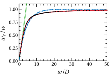
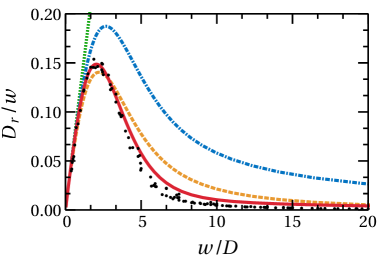
Figure 1: Scaled stretching rate $w_{r}/w$ versus $w/D$. The numerical results (black symbols) are based on simulations with 2000 realizations. The lines are for the naive result Eq.​​ (8) (green dotted); the exact result Eq.​​ (23) (red solid); and its practical approximation Eq.​​ (24) (blue dashed-dotted). For large values of $w/D$ we get $w_{r}/w=1$, as for a pure stretch.

Figure 2: Scaled diffusion coefficient $D_{r}/w$ versus $w/D$. The numerical results (black symbols) are based on simulations with 2000 realizations. The lines are for the naive result Eq.​​ (9) (green dotted); the exact result Eq.​​ (33) (red solid); and the approximation Eq.​​ (28) with ${\tau=1/(2D)}$ (blue dashed-dotted), and with Eq.​​ (34) (dashed orange line).

Below we are not using a matrix language, but address directly the statistical properties of an evolving distribution. In ${(\varphi,r)}$ polar coordinates Eq.​​ (1) takes the form

$$\dot{\varphi} \ =\ -w\sin(2\varphi)\ +\ \omega(t)$$ (12)

$$\dot{r} \ =\ [w\cos(2\varphi)]\ r$$ (13)

We see the equation for the phase decouples, while for the radius

$$\frac{d}{dt}\ln(r(t))\ \ =\ \ w\cos(2\varphi)$$ (14)

The RHS has some finite correlation time ${\tau\sim 1/D}$, and therefore $\ln(r)$ is like a sum of $t/\tau$ uncorrelated random variables. It follows from the central limit theorem that for long time the main body of the $\ln(r)$ distribution can be approximated by a normal distribution, with some average ${\mu\propto t}$, and some variance ${\sigma^{2}\propto t}$. Consequently we can define a radial stretching rate $w_{r}$ and a radial diffusion coefficient $D_{r}$ via Eq.​​ (6).

Our objective is to find explicit expression for $w_{r}$ and $D_{r}$, and also to characterize the full statistics of $r(t)$ in terms of the bare model parameters ${(w,D)}$. We shall see that the statistics of $r(t)$ is described by a bounded lognormal distribution.

Some rough estimates are in order. For large $D$ one naively assumes that due to ergodization of the phase ${\mu=\left\langle\cos(2\varphi)\right\rangle w}$ is zero, while ${\sigma^{2}\sim(w\tau)^{2}(t/\tau)}$. Hence one deduces that ${w_{r}\rightarrow 0}$ while ${D_{r}\propto w^{2}/D}$. A more careful approach KhripkovVardiCohen2012 that takes into account the non-isotropic distribution of the phase gives the asymptotic results Eq.​​ (8) and Eq.​​ (9). The dimensionless parameter that controls the accuracy of this result is $w/D$. These approximations are satisfactory for ${w/D\ll 1}$, and fails otherwise, see Fig.​​ 2 and Fig.​​ 2. For large $w/D$ we get $w_{r}\rightarrow w$, while $D_{r}\rightarrow 0$.

IV Phase ergodization

The Fokker-Planck equation (FPE) that is associated with Eq.​​ (12) is

$$\frac{\partial\rho}{\partial t}\ =\ \frac{\partial}{\partial\varphi}\left[\left(D\frac{\partial}{\partial\varphi}+w\sin(2\varphi)\right)\rho\right]$$ (15)

It has the canonical steady state solution

$$\rho_{\infty}(\varphi)\ \ \propto\ \ \exp\left[\frac{w}{2D}\cos(2\varphi)\right]$$ (16)

If we neglect the cosine potential in Eq.​​ (15) then the time for ergodization is ${\tau_{\text{erg}}\sim 1/D}$. But if $w/D$ is large we have to incorporate an activation factor, accordingly

$$\tau_{\text{erg}}\ \ =\ \ \frac{1}{D}\ \exp\left[\frac{w}{D}\right]$$ (17)

Fig.​​ 3(a) shows the distribution of the phase for two different initial conditions, as obtained by a finite time numerical simulation. It is compared with the steady state solution. The dynamics of $r$ depends only on $2\varphi$, and is dominated by the distribution at the vicinity of $\cos(2\varphi)\sim 1$. We therefore display in Fig.​​ 3(b) the distribution of $\varphi$ modulo $\pi$. We deduce that the transient time of the $\ln(r)$ spreading is much shorter than $\tau_{\text{erg}}$.

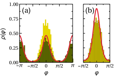
Figure 3: (a) Phase distribution for $(w/D)=10/3$ after time $(wt)=6$, with initial conditions $\varphi=0$ (filled, yellow) and $\varphi=\pi/2$ (green bars) with 2000 realizations. For larger times, both reach the steady state of Eq.​​ (16) (red line). (b) The distributions of $\varphi$ modulo $\pi$.

For the later calculation of $w_{r}$ we have to know the moments of the angular distribution. From Eq.​​ (16) we obtain:

$$X_{n}\ \ \equiv\ \ \left\langle\cos(2n\varphi)\right\rangle_{\infty}\ \ =\ \ \frac{I_{n}\left(\frac{w}{2D}\right)}{I_{0}\left(\frac{w}{2D}\right)}$$ (18)

Here $I_{n}(z)$ are the modified Bessel functions. For small $z$ we have ${I_{n}(z)\approx[1/n!](z/2)^{n}}$, while for large $z$ we have ${I_{n}(z)\approx(2\pi z)^{-1/2}e^{z}}$. The dependence of the $X_{n}$ on $n$ for representative values of $w/D$ is illustrated in the upper panel of Fig.​​ 4.

For the later calculation of $D_{r}$ we have to know also the temporal correlations. We define

$${}C_{n}(t)=\left\langle\cos(2n\varphi_{t})\cos(2\varphi)\right\rangle_{\infty}-X_{n}X_{1}\ \$$ (19)

where a constant is subtracted such that $C_{n}(\infty)=0$. We use the notations

$$c_{n}\ \ \equiv\ \ \int_{0}^{\infty}C_{n}(t)dt$$ (20)

and

$$\Delta_{n}\ \equiv\ C_{n}(0)\ =\ \frac{1}{2}\left(X_{n+1}+X_{n-1}\right)-X_{n}X_{1}\ \ \ \$$ (21)

In order to find an asymptotic expression we use

$$I_{n}(z)\approx\frac{e^{z}}{\sqrt{2\pi z}}\left[1-\frac{4n^{2}{-}1}{(8z)}+\frac{(4n^{2}{-}1)(4n^{2}{-}9)}{2(8z)^{2}}\right]$$

and get

$${}\Delta_{n}\ \approx\ 2\left(\frac{w}{D}\right)^{-2}n^{2}\ \ \ \ \ \ \ \mbox{for}\ \ \left(\frac{w}{D}\right)\gg 1$$ (22)

The dependence of the $\Delta_{n}$ on $n$ for representative values of $w/D$ is illustrated in the lower panel of Fig.​​ 4.

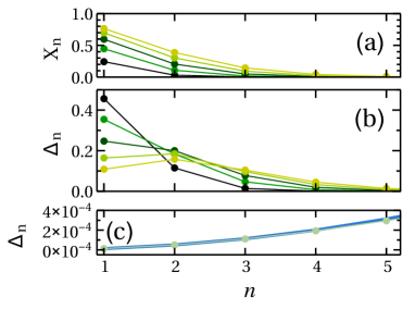
Figure 4: (a) The values of $X_{n}$ versus $n$ for some values of $w/D$. From bottom to top ${w/D=1,2,3,4,5}$. (b) The values of $\Delta_{n}$ versus $n$ for the same values of $w/D$, from top to bottom at $n{=}1$. (c) $\Delta_{n}$ versus $n$ for large $w/D$. Here $w/D=400$. The asymptotic approximation Eq.​​ (22) is indicated by blue line.

V Radial spreading

If follows from Eq.​​ (14) that the radial stretching rate is

$${}w_{r}\ \ =\ \ w\left\langle\cos(2\varphi)\right\rangle_{\infty}\ \ =\ \ X_{1}w$$ (23)

A rough interpolation for $X_{1}$ that is based on the asymptotic expressions for the Bessel functions in Eq.​​ (18) leads to the following approximation

$$w_{r}\ \ \approx\ \ \ w\left[1-\exp\left(-\frac{w}{4D}\right)\right]$$ (24)

The exact result as well as the approximation are illustrated in Fig.​​ 2 and compared with the results of numerical simulations.

For the second moment it follows from Eq.​​ (14) that the radial diffusion coefficient is

$$D_{r}\ \ =\ \ w^{2}\int_{0}^{\infty}C_{1}(t)dt\ \ =\ \ c_{1}w^{2}$$ (25)

If we assume that the ergodic angular distribution is isotropic, the calculation of $C_{1}(t)$ becomes very simple, namely,

$$C_{1}(t)\ =\ \frac{1}{2}\left\langle\cos{2(\varphi_{t}-\varphi_{0})}\right\rangle\ =\ \frac{1}{2}\mathrm{e}^{-4D|t|}$$ (26)

This expression implies a correlation time ${\tau=1/(2D)}$, such that ${c_{1}=(1/2)\Delta_{1}\tau}$ is half the “area” of the correlation function whose “height” is ${\Delta_{1}=1/2}$. Thus we get for the radial diffusion coefficient ${D_{r}=w^{2}/(8D)}$.

But in fact the ergodic angular distribution is not isotropic, meaning that $X_{1}$ is not zero, and ${\Delta_{1}<1/2}$. If $w$ is not too large we may assume that the correlation time $\tau$ is not affected. Then it follows that a reasonable approximation for the correlation function is

$$C_{1}(t)\ \ \approx\ \Delta_{1}\mathrm{e}^{-2|t|/\tau}$$ (27)

leading to

$$D_{r}\ \ \approx\ \ \frac{1}{2}\Delta_{1}\tau w^{2}\ \ =\ \ \Delta_{1}\frac{w^{2}}{4D}$$ (28)

This approximation is compared to the exact result that we derive later in Fig.​​ 2. Unlike the rough approximation ${D_{r}=w^{2}/(8D)}$, it captures the observed non-monotonic dependence of $D_{r}$ versus $w$, but quantitatively it is an over-estimate.

VI The exact calculation of the diffusion coefficient

We now turn to find an exact expression for the diffusion coefficient Eq.​​ (25) by calculating $c_{1}$ of Eq.​​ (20). Propagating an initial distribution ${\rho_{0}(\varphi)}$ with the FPE Eq.​​ (15) we define the moments:

$$x_{n}\ = \ \left\langle\cos(2n\,\varphi_{t})\right\rangle_{0}\ =\ \left\langle\cos(2n\,\varphi)\right\rangle_{t}$$

$$= \ \int\cos(2n\,\varphi)\ \rho_{t}(\varphi)d\varphi$$ (29)

The moments equation of motion resulting from the FPE is risken1984fokker :

$$\frac{d}{dt}x_{n}\ \ =\ \ -\Lambda_{n}\,x_{n}\ +\ W_{n}\left(x_{n-1}-x_{n+1}\right)$$ (30)

where ${\Lambda_{n}=4Dn^{2}}$ and $W_{n}=wn$. Due to ${\Lambda_{0}=W_{0}=0}$ the zeroth moment ${x_{0}=1}$ does not change in time. Thus the rank of Eq.​​ (30) is less than its dimension reflecting the existence of a zero mode $x_{n}=X_{n}$ that corresponds to the steady state of the FPE. We shall use the subscript ”$\infty$” to indicate the steady state distribution. Any other solution $x_{n}(t)$ goes to $X_{n}$ in the long time limit, while all the other modes are decaying. To find $X_{n}$ the equation should be solved with the boundary condition ${X_{\infty}=0}$, and normalized such that ${X_{0}=1}$. Clearly this is not required in practice: because we already know the steady state solution Eq.​​ (15), hence Eq.​​ (18).

We define $x_{n}(t;\varphi_{0})$ as the time-dependent solution for an initial preparation ${\rho_{0}(\varphi)=\delta(\varphi-\varphi_{0})}$. Then we can express the correlation function of Eq.​​ (19) as follows:

$$C_{n}(t)\ =\ \left\langle x_{n}(t;\varphi)\cos(2\varphi)\right\rangle_{\infty}-X_{n}X_{1}$$ (31)

By linearity the $C_{n}(t)$ obey the same equation of motion as that of the $x_{n}(t)$, but with the special initial conditions ${C_{n}(0)=\Delta_{n}}$. Note that ${C_{0}(t)=0}$ at any time. In the infinite time limit ${C_{n}(\infty)=0}$ for any $n$.

Our interest is in the area $c_{n}$ as defined in Eq.​​ (20). Writing Eq.​​ (30) for $C_{n}(t)$, and integrating it over time we get

$${}\Lambda_{n}\,c_{n}\ -\ W_{n}\left(c_{n-1}-c_{n+1}\right)\ \ =\ \ \Delta_{n}$$ (32)

This equation should be solved with the boundary conditions ${c_{0}=0}$ and ${c_{\infty}=0}$. The solution is unique because the $n=0$ site has been effectively removed, and the truncated matrix is no longer with zero mode. One possible numerical procedure is to start iterating with $c_{1}$ as initial condition, and to adjust it such that the solution will go to zero at infinity. An optional procedure is to integrate the recursion backwards as explained in the next section. The bottom line is the following expression

$$D_{r}\ \ =\ \ c_{1}w^{2}\ \ =\ \ -\sum_{n=1}^{\infty}\frac{(-1)^{n}}{n}\Delta_{n}X_{n}w$$ (33)

where $X_{n}$ and $\Delta_{n}$ are given by Eq.​​ (18) and Eq.​​ (21) respectively.

The leading term approximation ${D_{r}\approx\Delta_{1}X_{1}w}$ is consistent with the heuristic expression ${D_{r}\approx(1/2)\Delta_{1}\tau w^{2}}$ of Eq.​​ (28) upon the identification

$$\tau\ \ =\ \ \frac{2}{w}\left[1-\exp\left(-\frac{w}{4D}\right)\right]$$ (34)

This expression reflects the crossover from diffusion-limited (${\tau\propto 1/D}$) to drift-limited (${\tau\propto 1/w}$) spreading. Fig.​​ 2 compares the approximation that is based on Eq.​​ (28) with Eq.​​ (34) to the exact result Eq.​​ (33).

In the limit $(w/D)\rightarrow 0$ the asymptotic result for the radial diffusion coefficient is ${D_{r}=w^{2}/(8D)}$. We now turn to figure out what is the asymptotic result in the other extreme limit ${(w/D)\rightarrow\infty}$. The large $w/D$ approximation that is based on the first term of Eq.​​ (33), with the limiting value ${X_{1}=1}$, provides the asymptotic estimate ${D_{r}\approx 2D^{2}/w}$. This expression is based on the asymptotic result Eq.​​ (22) for $\Delta_{n}$ with ${n=1}$. In fact we can do better and add all the higher order terms. Using Abel summation we get

$$D_{r}\ =\ 2\frac{D^{2}}{w}\sum_{n=1}^{\infty}(-1)^{n{-}1}n\ =\ \frac{1}{2}\frac{D^{2}}{w}$$ (35)

Thus the higher order terms merely add a factor $1/4$ to the asymptotic result. If we used Eq.​​ (28), we would have obtained the wrong prediction $D_{r}\approx D/2$ that ignores the $\tau$ dependence of Eq.​​ (34).

VII Derivation of the recursive solution

In this section we provide the details of the derivation that leads from Eq.​​ (32) to Eq.​​ (33). We define ${W_{n}^{\pm}=\mp W_{n}}$ and rewrite the equation in the more general form

$$-W_{n}^{+}c_{n+1}+\Lambda_{n}c_{n}-W_{n}^{-}c_{n-1}\ =\ \Delta_{n}$$ (36)

A similar problem was solved in Coffey1993 , while here we present a much simpler treatment. First we solve the associated homogeneous equation. The solution $c_{n}=X_{n}$ satisfies

$$-W_{n}^{+}X_{n+1}+\Lambda_{n}X_{n}-W_{n}^{-}X_{n-1}\ =\ 0$$ (37)

and one can define the ratios ${R_{n}=X_{n}/X_{n-1}}$. Note that these ratios satisfies a simple first-order recursive relation. However we bypass this stage because we can extract the solution from the steady state distribution.

We write the solution of the non-homogeneous equation as

$$c_{n}\ \ :=\ \ X_{n}\tilde{c}_{n}$$ (38)

and we get the equation

$$-W_{n}^{+}X_{n+1}\tilde{c}_{n+1}+\Lambda_{n}X_{n}\tilde{c}_{n}-W_{n}^{-}X_{n-1}\tilde{c}_{n-1}\ =\ \Delta_{n}$$

Clearly it can be re-written as

$$-W_{n}^{+}X_{n+1}(\tilde{c}_{n+1}-\tilde{c}_{n})+W_{n}^{-}X_{n-1}(\tilde{c}_{n}-\tilde{c}_{n-1})\ =\ \Delta_{n}$$

We define the discrete derivative

$$\tilde{a}_{n}\ \ :=\ \ \tilde{c}_{n}-\tilde{c}_{n-1}$$ (39)

And obtain a reduction to a first-order equation:

$$-W_{n}^{+}X_{n+1}\tilde{a}_{n+1}+W_{n}^{-}X_{n-1}\tilde{a}_{n}\ =\ \Delta_{n}$$ (40)

This can be re-written in a simpler way by appropriate definition of scaled variables. Namely, we define the notations

$$\tilde{R}_{n}\ =\ \frac{W_{n}^{+}}{W_{n}^{-}}R_{n}\hskip 56.9055pt\tilde{\Delta}_{n}\ =\ \frac{\Delta_{n}}{W_{n}^{+}}$$ (41)

and the rescaled variable

$$a_{n}\ \ :=\ \ X_{n}\tilde{a}_{n}$$ (42)

and then solve the $a_{n}$ recursion in the backwards direction:

$$a_{\infty}=0;\ \ \ \ a_{n}=\tilde{R}_{n}\left[\tilde{\Delta}_{n}+a_{n+1}\right]$$ (43)

If all the $R_{n}$ were unity it would imply that $a_{1}-a_{\infty}$ equals $\sum\Delta_{n}$. So it is important to verify that the ”area” converges. Next we can solve in the forward direction the $c_{n}$ recursion for the non-homogeneous equation, namely,

$$c_{0}=0;\ \ \ \ \ c_{n}=R_{n}c_{n-1}+a_{n}$$ (44)

In fact we are only interested in

$$c_{1}\ \ =\ \ a_{1}\ \ =\ \ \tilde{R}_{1}\tilde{\Delta}_{1}+\tilde{R}_{1}\tilde{R}_{2}\tilde{\Delta}_{2}+...$$ (45)

Note that in our calculation the $\tilde{R}_{n}=-R_{n}$, and therefore ${\tilde{R}_{1}\cdots\tilde{R}_{n}=(-1)^{n}X_{n}}$.

VIII The moments of the radial spreading

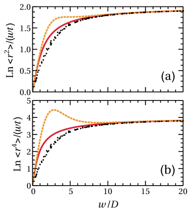
Figure 5: Scaled moments versus $w/D$. The red solid lines are the exact results for the 2nd and 4th moments, given by Eq.​​ (48) and Eq.​​ (70), and the large $w/D$ asymptotic values are at $2$ and $4$, respectively. These are compared with the numerical results (black symbols), and contrasted with the Lognormal prediction (orange dashed lines). The later provides an overestimate for intermediate values of $w/D$.

The moments of a lognormal distribution are given by the following expression

$${}\ln\langle r^{n}\rangle\ \ =\ \ \mu n\ +\ \frac{1}{2}\sigma^{2}n^{2}$$ (46)

On the basis of the discussion after Eq.​​ (14), if one assumed that the radial spreading at time $t$ could be globally approximated by the lognormal distribution (tails included), it would follow that

$${}\frac{d}{dt}\ln\langle r^{n}\rangle\ \ =\ \ nw_{r}+n^{2}D_{r}$$ (47)

In Fig.​​ 5 we plot the lognormal-based expected growth-rate of the 2nd and the 4th moments as a function of $w/D$. For small $w/D$ there is a good agreement with the expected results, which are $w^{2}/D$ and $3w^{2}/D$ respectively. For large $w/D$ the dynamics is dominated by the stretching, meaning that $w_{r}\approx w$, while ${D_{r}\rightarrow 0}$, so again we have a trivial agreement. But for intermediate values of $w/D$ the lognormal moments constitute an overestimate when compared with the exact analytical results that we derive in the next section. In fact also the exact analytical result looks like an overestimate when compared with the results of numerical simulations. But the latter is clearly a sampling issue that is explained in Appendix D.

The deviation of the lognormal moments from the exact results indicates that the statistics of large deviations is not captured by the central limit theorem. This point is illuminated in Fig.​​ 6. The Gaussian approximation constitutes a good approximation for the body of the distribution but not for the tails that dominate the moment-calculation. Clearly, the actual distribution can be described as a bounded lognormal distribution, meaning that it has a natural cutoff which is implied by the strict inequality ${w_{r}<w}$. The stretching rate cannot be faster than $w$. But in fact, as observed in Fig.​​ 6b, the deviation from the lognormal distribution happens even before the cutoff is reached.

Below we carry out an exact calculation for the 2nd and 4th moments. In the former case we show that

$${}\frac{d}{dt}\ln\langle r^{2}\rangle\ \ \sim\ \ 2\left((w^{2}+D^{2})^{1/2}-D\right)$$ (48)

This agrees with the lognormal-based prediction $w^{2}/D$ for ${(w/D)\ll 1}$, and goes to $2w$ for ${(w/D)\gg 1}$, as could be anticipated.

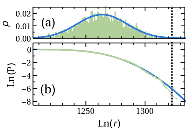
Figure 6: (a) Distribution of $\ln(r)$ for $w/D=10/3$ after time $wt=2000$ with initial conditions $r=1$ and $\varphi=0$. Numerical results (green histogram), that are based on $2000$ realizations, are fitted to a Gaussian distribution (blue line).   (b) Inverse cumulative probability of the same distribution. The black dotted line indicate the numerically determined value ${\ln\left\langle r^{2}\right\rangle^{1/2}\approx 1323}$. This value is predominated by the tail of the distribution. The Gaussian fit fails to reproduce this value, and provides a gross over-estimate ${\ln\left\langle r^{2}\right\rangle^{1/2}\approx 1701}$.

Before we go the derivation of this result we would like to illuminates its main features by considering a simple-minded reasoning. Let us ask ourselves what would be the result if the spreading was isotropic ($w_{r}=0$). In such case the moments of spreading can be calculated as if we are dealing with the multiplication of random numbers. Namely, assuming that the duration of each step is ${\tau=1/(2D)}$, and treating $t$ as a discrete index, Eq.​​ (13) implies that the spreading is obtained by multiplication of uncorrelated stretching factors ${\exp[w\tau\cos(\varphi)]}$. Each stretching exponent has zero mean and dispersion ${\sigma_{1}^{2}=(1/2)[w\tau]^{2}}$, which implies $D_{r}=\sigma_{1}^{2}/(2\tau)$. Consequently we get for the moments

$$\langle r^{n}\rangle\ \ =\ \ \left[\left\langle\mathrm{e}^{nw\tau\cos(2\varphi)}\right\rangle\right]^{t/\tau}\ r_{0}^{n}$$ (49)

leading to

$${}\frac{d}{dt}\ln\langle r^{n}\rangle\ \ =\ \ \dfrac{1}{\tau}\ln\left[I_{0}\left(\sqrt{2}n\sigma_{1}\right)\right]$$ (50)

This gives a crossover from $n^{2}D_{r}$ for ${\sigma_{1}\ll 1}$ to $nw$ for ${\sigma_{1}\gg 1}$, reflecting isotropic lognormal spreading in the former case, and pure stretching in the latter case. So again we see that the asymptotic limits are easily understood, but for the derivation of the correct interpolation, say Eq.​​ (48), further effort is required.

IX The exact calculation of the moments

We turn to perform an exact calculation of the moments. One can associate with the Langevin equation Eq.​​ (1) an FPE for the distribution, and from that to derive the equation of motion for the moments. The procedure is explained and summarized in Appendix E. For the first moments we get

$$\frac{d}{dt}\left\langle x\right\rangle = w\left\langle x\right\rangle-D\left\langle x\right\rangle$$ (51)

$$\frac{d}{dt}\left\langle y\right\rangle = -w\left\langle y\right\rangle-D\left\langle y\right\rangle$$ (52)

with the solution

$$\left\langle x\right\rangle = x_{0}\,\exp[-(D-w)t]$$ (53)

$$\left\langle y\right\rangle = y_{0}\,\exp[-(D+w)t]$$ (54)

For the second moments

$$\frac{d}{dt}\left(\begin{array}[]{c}\left\langle x^{2}\right\rangle\\ \left\langle y^{2}\right\rangle\end{array}\right) = \Big{[}-2D+2D\bm{\sigma}_{1}+2w\bm{\sigma}_{3}\Big{]}\left(\begin{array}[]{c}\left\langle x^{2}\right\rangle\\ \left\langle y^{2}\right\rangle\end{array}\right)\ \ \ \$$ (59)

$$\frac{d}{dt}\left\langle xy\right\rangle\ \ = -4D\left\langle xy\right\rangle$$ (60)

where $\bm{\sigma}$ are Pauli matrices. The solution is:

$$\left(\begin{array}[]{c}\left\langle x^{2}\right\rangle\\ \left\langle y^{2}\right\rangle\\ \left\langle xy\right\rangle\end{array}\right)=\left[\begin{matrix}e^{-2Dt}\bm{M}&0\cr 0&e^{-4Dt}\end{matrix}\right]\left(\begin{array}[]{c}x_{0}^{2}\\ y_{0}^{2}\\ x_{0}y_{0}\end{array}\right)$$ (67)

where $\bm{M}$ is the following matrix:

$$\cosh[2(w^{2}{+}D^{2})^{1/2}t]+\sinh[2(w^{2}{+}D^{2})^{1/2}t]\frac{D\bm{\sigma}_{1}+w\bm{\sigma}_{3}}{\sqrt{w^{2}{+}D^{2}}}$$

For an initial isotropic distribution we get ${\langle r^{2}\rangle_{t}=Mr_{0}^{2}}$, where

$${}M = e^{-2Dt}\cosh[2(w^{2}+D^{2})^{1/2}t]$$

$$+\frac{D}{\sqrt{w^{2}+D^{2}}}e^{-2Dt}\sinh{[2(w^{2}+D^{2})^{1/2}}t]$$

The short time $t$ dependence is quadratic, reflecting “ballistic” spreading, while for long times

$$\left\langle r^{2}\right\rangle_{t} \approx \frac{r_{0}^{2}}{2}\ \left(1+\frac{D}{\sqrt{w^{2}{+}D^{2}}}\right)\times$$ (69)

$$\ \exp\left[2\left((w^{2}+D^{2})^{1/2}-D\right)t\right]\ \ \ \$$

From here we get Eq.​​ (48). For the 4th moments the equations are separated into two blocks of even-even powers and odd-odd powers in $x$ and $y$. For the even block:

$$\frac{d}{dt}\begin{pmatrix}\left\langle x^{4}\right\rangle\\ \left\langle x^{2}y^{2}\right\rangle\\ \left\langle y^{4}\right\rangle\\ \end{pmatrix}\ =\ 2\tilde{\bm{M}}\begin{pmatrix}\left\langle x^{4}\right\rangle\\ \left\langle x^{2}y^{2}\right\rangle\\ \left\langle y^{4}\right\rangle\\ \end{pmatrix}$$ (70)

where

$$\tilde{\bm{M}}\ =\ \begin{pmatrix}2(w{-}D)&6D&0\\ D&-6D&D\\ 0&6D&-2(w{+}D)\\ \end{pmatrix}$$ (71)

The eigenvalues of this matrix are the solution of $\lambda^{3}+10D\lambda^{2}+(16D^{2}-4w^{2})\lambda-24Dw^{2}=0$. There are two negative roots, and one positive root. For small $w/D$ the latter is ${\lambda\approx(3/2)(w^{2}/D)}$, and we get that the growth-rate is ${3w^{2}/D}$ as expected from the log-normal statistics.

X Discussion

In this work we have studied the statistics of a stochastic squeeze process, defined by Eq.​​ (1). Consequently we are able to provide a quantitatively valid theory for the description of the noise-affected decoherence process in bimodal Bose-Einstein condensates, aka QZE. As the ratio $w/D$ is increased, the radial diffusion coefficient of $\ln(r)$ changes in a non-monotonic way from ${D_{r}=w^{2}/(8D)}$ to ${D_{r}=D^{2}/(2w)}$, and the non-isotropy is enhanced, namely the average stretching rate increases from ${w_{r}=w^{2}/(4D)}$ to the bare value ${w_{r}=w}$. The analytical results Eq.​​ (23) and Eq.​​ (33) are illustrated in Fig.​​ 2 and Fig.​​ 2,

Additionally we have solved for the moments of $r$. One observes that the central limit theorem is not enough for this calculation, because the moments are predominated by the non-Gaussian tails of the $\ln(r)$ distribution. In particular we have derived for the second moment the expression ${\langle r^{2}\rangle_{t}=Mr_{0}^{2}}$ with $M$ that is given by Eq.​​ (IX), or optionally one can use the practical approximation Eq.​​ (48).

The main motivation for our work comes form the interest in the BJJ. Form mathematical point of view the BJJ can be regarded as a quantum pendulum. It has both stable and unstable fixed points. Its dynamics has been explored by numerous experiments. We mention for example Ref.Oberthaler2005 who observed both Josephson oscillations (“liberations”) and self trapping (“rotations”), and Ref.Steinhauer2007 who observed the a.c. and the d.c. Josephson effects. The phase-space of the device is spherical, known as the Bloch sphere. A quantum state corresponds to a quasi-distribution (Wigner function) on that sphere, and can be characterized by the Bloch vector $\vec{S}$. The length $\mathcal{F}=\left|\vec{S}\right|$ of the Bloch vector reflects the one-body coherence, and has to do with the “fringe visibility” in a “time-of-flight” measurement. If all the particles are initially condensed in the upper orbital of the BJJ, it corresponds to a coherent ${\mathcal{F}=1}$ wavepacket that is positioned on top of the hyperbolic point, which corresponds to the upper position of the pendulum. The dynamics has been thoroughly analyzed in Chuchem10 and experimentally demonstrated in chapman .

To the best of our knowledge neither the Kapitza effect kapitza nor the Zeno effect have been demonstrated experimentally in the BJJ context. We expect the decay of $\mathcal{F}$ to be suppressed due to the periodic or the noisy driving, respectively. Let us clarify the experimental significance of our results for the full statistics of the radial spreading in the latter case. In order to simplify the discussion, let us assume that the definition of $\mathcal{F}$ is associated with the measurement of a single coordinate $\hat{x}$. Measurement of $\hat{x}$ is essentially the same as probing an occupation difference. In a semiclassical perspective (Wigner function picture) the phase-space coordinate $x$ satisfies Eq.​​ (1), where $\omega(t)$ arises from frequent interventions, or measurements, or noise that comes from the surrounding. Using a Feynman-Vernon perspective, each $x$ outcome of the experiment can be regarded as the result of one realization of the stochastic process. The “coherence” is determined by the second moment of $\hat{x}$. But it is implied by our discussion of the sampling problem that it is impractical to determine this second moment from any realistic experiment (rare events are not properly accounted). The reliable experimental procedure would be to keep the full probability distribution of the measured $x$ variable, and to extract the $\mu$ and the $\sigma$ that characterize its lognormal statistics. For the latter we predict non-trivial dependence on $w/D$.

Still, from purely mathematical point of view, one might be curious about the validity of the heuristic QZE expression Eq.​​ (4). We already pointed out in the Introduction that the lognormal assumption implies that it should be replaced by Eq.​​ (7), which reduce to Eq.​​ (4) only for short times if the noise is very strong (small $w/D$). We note that the expression that has been advertised originally in KhripkovVardiCohen2012 was slightly different, namely,

$${}\mathcal{S}(t)\ =\ e^{4D_{r}t}\cosh(2w_{r}t)-1$$ (72)

The difference is due to the assumption (there) that it is $\alpha$, as defined in Appendix A, rather than $r$ that has a lognormal distribution. In physical terms it is like ignoring the initial isotropy of the preparation, hence creating an artifact - an artificial transient. In any case we found in the present work that none of these expressions are correct. This is because the tail of the distribution is bounded. From Eq.​​ (48) we deduce that a practical approximation would be

$${}\mathcal{S}(t)\ =\ 2\left((w^{2}+D^{2})^{1/2}-D\right)\,t$$ (73)

Note that both expression Eq.​​ (7) and Eq.​​ (73) agrees with the heuristic expectation $(w^{2}/D)t$ for ${(w/D)\ll 1}$, and goes to bare non-suppressed value $2wt$ for ${(w/D)\gg 1}$. The difference between them is for intermediate values of $w/D$ where the lognormal prediction is an overestimate. On the other hand, in a realistic experiment, we expect an underestimate as illustrated in Fig.​​ 5.

Appendix A The squeeze operation

The squeeze operation is described by a real symplectic matrix that has unit determinant and trace ${|a|>2}$. Any such matrix can be expressed as follows:

$$\bm{U}\ =\ \left(\begin{matrix}a&b\\ c&d\end{matrix}\right)\ =\ \pm\mathrm{e}^{\alpha\bm{H}}\ \ \ \ \ \ \ \ [ad-cb=1]$$ (74)

where $\bf{H}$ is a real traceless matrix that satisfies ${\bm{H}^{2}=1}$. Hence it can be expressed as a linear combination of the three Pauli matrices:

$$\bm{H}\ =\ n_{1}\bm{\sigma}_{1}+in_{2}\bm{\sigma}_{2}+n_{3}\bm{\sigma}_{3}\ \ \ \$$ (75)

with ${n_{1}^{2}-n_{2}^{2}+n_{3}^{2}=1}$. Consequently

$$\bm{U}\ \ =\ \ \pm\left[\cosh(\alpha)\bm{1}+\sinh(\alpha)\bm{H}\right]$$ (76)

We define the canonical form of the squeeze operation as

$$\bm{\Lambda}\ \ =\ \ \left(\begin{matrix}\exp(\alpha)&0\\ 0&\exp(-\alpha)\end{matrix}\right)$$ (77)

Then we can obtain any general squeeze operation via similarity transformation that involves re-scaling of the axes and rotation, and on top an optional reflection.

We can operate with $\bm{U}$ on an initial isotropic cloud that has radius ${r_{0}=1}$. Then we get a stretched cloud that has spread ${\left\langle r^{2}\right\rangle=\mathcal{A}\,r_{0}^{2}}$, where

$${}\mathcal{A}\ \ \equiv\ \ \left.\left\langle r^{2}\right\rangle\right|_{r_{0}{=}1}\ \ =\ \ \cosh(2\alpha)$$ (78)

We also define the “spreading” as

$$\mathcal{S}\ \ =\ \ \mathcal{A}-1\ \ =\ \ 2\sinh^{2}(\alpha)$$ (79)

The notation $\alpha$ has no meaning for a stochastic squeeze process, while the notation ${\mathcal{A}\equiv\left\langle r^{2}\right\rangle}$ still can be used. In the latter case the average is over the initial conditions and also over realizations of $\omega(t)$, implying that in Eq.​​ (78) the $\cosh(2\alpha)$ should be averaged over $\alpha$.

Appendix B Numerical simulations

There are numerous numerical schemes that allow the simulation of a Langevin Equation. For example, the Milstein, the Runge-Kutta, and higher-order approximations such as the truncated Taylor expansion KP . These schemes are based on iterative integration of the Langevin equation, then Taylor expand the solution in small $dt$. The dynamics generated by Eq.​​ (1) is symplectic, however the numerical methods listed above do not respect this constraint. Instead one can exploit the linear nature of the problem. Namely, Eq.​​ (1) is re-written as

$$\dot{\bm{r}}_{t}=\bm{H}(t)\bm{r}_{t}$$ (80)

$$\bm{H}=\bm{H}_{s}+\bm{H}_{r}(t)$$ (81)

Where $\bm{H}_{s}$ and $\bm{H}_{r}$ are the generators of the stretching and the angular diffusion, respectively, while $\bm{r}_{t}=(x_{t},y_{t})$. If $\bm{H}_{r}$ were constant, the solution of Eq.​​ (80) would be obtained by simple exponentiation of $\bm{H}$, namely $\bm{r}_{t_{f}}=\bm{U}\bm{r}_{0}$, with $\bm{U}=\exp[(\bm{H}_{r}+\bm{H}_{s})t_{f}]$. Choosing a small enough time interval $dt$ and using the Suzuki-Trotter formula, the latter equation is approximated by

$$\bm{U}=\bm{U}_{t_{f}}\cdots\bm{U}_{3dt}\bm{U}_{2dt}\bm{U}_{dt}$$ (82)

$$\bm{U}_{t}=\exp{(\bm{H}_{s}dt)}\exp{(\bm{H}_{r}dt)}$$ (83)

Where $\bm{U}_{t}$ gives the evolution of the vector $\bm{r}_{t}$ for small time $dt$, namely, ${\bm{r}_{t}=\bm{U}_{t}\bm{r}_{t-dt}}$. Eq.​​ (82) is valid also for time dependent $\bm{H}$, where the small step evolution Eq.​​ (83) takes the form

$$\bm{U}_{t}\ \ =\ \ \left(\begin{matrix}e^{w\,dt}&0\\ 0&e^{-w\,dt}\end{matrix}\right)\ \left(\begin{matrix}\cos{\alpha_{t}}&-\sin{\alpha_{t}}\\ \sin{\alpha_{t}}&\cos{\alpha_{t}}\end{matrix}\right)$$ (84)

The uncorrelated random variables $\alpha_{t}$ have zero mean, and are taken from a box distribution of width $\sqrt{24D\,dt}$, such that their variance is ${2D\,dt}$. As a side note we remark that by Taylor expanding Eq.​​ (84) to second order in $dt$, the Milstein scheme is recovered. The radial coordinate $r$ is calculated under the assumption that the the preparation is ${(x_{0}{=}1,y_{0}{=}0)}$. Accordingly, what we calculate for each realization is

$${}r\ \ =\ \ \sqrt{U_{xx}^{2}+U_{yx}^{2}}$$ (85)

In Fig.​​ 7a we display the distribution of the trace $a$ for many realizations of such stochastic squeeze process. Rarely the result is a rotation, and therefore in the main text we refer to it as “squeeze”. From the trace we get the squeeze exponent $\alpha$, and from Eq.​​ (85) we get the radial coordinate $r$. The correlation between these two squeeze measures is illustrated in Fig.​​ 7b. For the long time simulations that we perform in order to extract various moments, we observe full correlation (not shown). In order to extract the various moments, we perform the simulation for a maximum time of $wt=7500$, with the initial condition $\bm{r}_{0}=(1,0)$.

We note that the results of Section IX for the evolution of the moments can be recovered by averaging over product of the evolution matrices. For the first moments we get the linear relation ${\left\langle\bm{r}_{t}\right\rangle=\left\langle\bm{U}\right\rangle\bm{r}_{0}}$, where

$$\left\langle\bm{U}\right\rangle\ \ = \ \ \left\langle...\ \bm{U}_{t_{3}}\ \bm{U}_{t_{2}}\ \bm{U}_{t_{1}}\right\rangle\ \ =\ \ \left[\left\langle\bm{U}_{t}\right\rangle\right]^{t/dt}$$ (86)

$$\ \ =\ \ \left(\begin{matrix}e^{-(D+w)t}&0\\ 0&e^{-(D-w)t}\end{matrix}\right)$$

Similar procedure can be applied for the calculation of the higher moments.

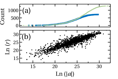
Figure 7: We consider 2000 realizations of a stochastic squeeze process. For each realization the trace ${a=\mbox{trace}(\bm{U})}$ is calculated. (a) The cumulative count of the $a$ values. Green points are for positive values, while blue rectangles are for negative values. Here ${(w/D)=10/3}$ and ${wt=40}$. For simulations with longer times the distribution of positive and negative values become identical (not shown). (b) Scatter plot of $|a|$ versus the radial coordinate $r$. For simulations with longer times we get full correlation.

Appendix C Relation to QZE

It is common to represent the quantum state of the bosonic Josephson junction by a Wigner function on the Bloch sphere, see Chuchem10 for details. A coherent state is represented by a Gaussian-like distribution, namely

$${}\rho^{(0)}(x,y)\ \ \approx\ \ 2\exp\left[-\frac{1}{\hbar}(x^{2}+y^{2})\right]$$ (87)

where $x$ and $y$ are local conjugate coordinates. The Wigner function is properly normalized with integration measure ${dxdy/(2\pi\hbar)}$. The dimensionless Plank constant is related to the number $N$ of Bonsons, namely ${\hbar=(N/2)^{-1}}$. After a squeeze operation one obtains a new state ${\rho^{(t)}(x,y)}$. The survival probability is

$${}\mathcal{P}(t)=\text{Tr}\,\left[\rho^{(0)}\rho^{(t)}\right]=\frac{1}{\cosh(\alpha)}=\frac{1}{1{+}\frac{1}{2}\mathcal{S}(t)}\ \$$ (88)

However it is more common, both theoretically and experimentally to quantify the decay of the initial state via the length of the Bloch vector, namely ${\mathcal{F}(t)=|\vec{S}(t)|}$. It has been explained in KhripkovVardiCohen2012 that

$${}\mathcal{F}(t)\approx\exp\left\{-\hbar\sinh^{2}(\alpha)\right\}=\exp\left\{-\frac{\hbar}{2}\mathcal{S}(t)\right\}\ \$$ (89)

Comparing with the short time approximation of Eq.​​ (88), namely ${\mathcal{P}\approx\exp[-(1/2)\mathcal{S}(t)]}$, note the additional $\hbar=2/N$ factor in Eq.​​ (89). This should be expected: the survival probability drops to zero even if a single particle leaves the condensate. Contrary to that, the fringe visibility reflects the expectation value of the condensate occupation, and hence its decay is much slower. Still both depend on the spreading ${\mathcal{S}(t)}$.

The dynamics that is generated by Eq.​​ (1) does not change the direction of the Bloch vector, but rather shortens its length, meaning that the one-body coherence is diminished, reflecting the decay of the initial preparation. Using the same coordinates as in KhripkovVardiCohen2012 the Bloch vector is ${\vec{S}(t)=(S,0,0)}$, hence all the information is contained in the measurement of a single observable, aka fringe visibility measurement.

For a noiseless canonical squeeze operation we have ${D=0}$ and ${\alpha=wt}$, hence one obtains ${\mathcal{S}(t)=2\sinh^{2}(wt)}$ which is quadratic for short times. In contrast to that, for a stochastic squeeze process Eq.​​ (89) should be averaged over realizations of $\omega(t)$. Thus $\mathcal{F}(t)$ is determined by the full statistics that we have studied in this paper.

At this point we would like to remind the reader what is the common QZE argument that leads to the estimate of Eq.​​ (4). One assumes that for strong ${D}$ the time for phase randomization is ${\tau=1/(2D)}$. Dividing the evolution into $\tau$-steps, and assuming that at the end of each step the phase is totally randomized (as in projective measurement) one obtains

$$\overline{\mathcal{A}(t)} \approx \left[\overline{\mathcal{A}(\tau)}\right]^{t/\tau}\ \ \approx\ \ \left[1-2(w\tau)^{2}\right]^{t/\tau}$$ (90)

$$\approx \ \ \exp\left[-(w^{2}/D)t\right]$$ (91)

The overline indicates average over realizations, as discussed after Eq.​​ (78). The short time expansion of exponent is linear rather than quadratic, and the standard QZE expression Eq.​​ (4) is recovered. This approximation is justified in the “Fermi Golden rule regime”, namely for ${\tau\ll t\ll t_{r}}$, during which the deviation from isotropy can be treated as a first-order perturbation. For longer times, and definitely for weaker noise, the standard QZE approximation cannot be trusted.

Appendix D Sample moments of a lognormal distribution

Consider a lognormal distribution of $r$ values. This mean that the $\ln r$ values have a Gaussian distribution. For a finite sample of $N$ values, one can calculate the sample average and the sample variance of the $\ln r$ values in order to get a reliable estimate for $\mu$ and $\sigma$, and then calculate the moments $\left\langle r^{n}\right\rangle$ via Eq.​​ (46). But a direct calculation of these moments provides a gross under-estimate as illustrated in Fig.​​ 8. This is because the direct average is predominated by rare values that belong to the tail of the distribution.

The lesson is that direct calculation of moments for log-wide distribution cannot be trusted. It can provide a lower bound to the true results, not an actual estimate.

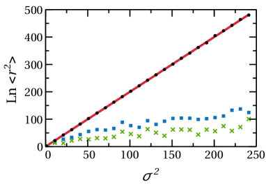
Figure 8: $\ln\left\langle r^{2}\right\rangle$ versus $\sigma$ for Lognormal distribution. Without loss of generality $\mu=0$. The true result is represented by red line. Numerical estimate based on $10^{2}$ and $10^{5}$ realizations are indicated by green crosses and blue rectangles, respectively. For the latter set of realization we get a much better estimate using an optional procedure (black dots). Namely, we calculate the sample average and the sample variance of the $\ln r$ values in order to determine $\mu$ and $\sigma$, and then use Eq.​​ (46) to estimate the moments.

Appendix E Fokker-Planck from Langevin equation

We provide a short derivation for the FPE that is associated with a given Langevin equation. From this we obtains the equations of motion for observables. For sake of generality we write the Langevin equation as follows:

$$\dot{x_{j}}\ =\ v_{j}+g_{j}\,\omega(t)\ \equiv\ f_{j}$$ (92)

$$\left\langle\omega(t)\omega(t^{\prime})\right\rangle\ =\ 2D\delta_{\tau}(t-t^{\prime})$$ (93)

The $v_{j}$ and the $g_{j}$ are some functions of the $x_{i}$. Eq.​​ (1) is obtained upon the identification ${x_{j}=(x,y)}$ and ${v_{j}=(wx,-wy)}$, and ${g_{j}=(-y,x)}$. The “noise” has zero average, namely $\left\langle\omega(t)\right\rangle=0$, and is characterized by a correlation time $\tau$. Accordingly the $\delta_{\tau}(t-t^{\prime})$ has a short but finite width, which is later taken to be zero.

For a particular realization of the noise, the continuity equation for the Liouville distribution $\rho(x)$ reads:

$$\frac{\partial\rho}{\partial t}\ \ =\ \ -\frac{\partial}{\partial x_{j}}\left(f_{j}\rho\right)$$ (94)

We are interested in $\rho(x)$ averaged over many-realizations of the noise $\omega$. In its current form Eq.​​ (94) cannot be averaged, because $\rho$ and $f$ are not independent variables. To overcome this issue Eq.​​ (94) is integrated iteratively. To second order one obtains

$$\rho(t+dt)-\rho(t)\ =\$$ (95)

$$-\int_{t}^{t{+}dt}\!\!\!\!\!dt^{\prime}\dfrac{\partial}{\partial x_{j}}f_{j}(t^{\prime})\left[\rho(t)-\int_{t}^{t^{\prime}}\!\!dt^{\prime\prime}\dfrac{\partial}{\partial x_{k}}f_{k}(t^{\prime\prime})\rho(t)\right]$$

Performing the average over realizations of the noise, non-vanishing noise-related term arise from the correlator of Eq.​​ (93). Then performing the $dt^{\prime\prime}$ integral over the broadened delta one obtains a $1/2$ factor. Dividing both sides by $dt$, and taking the limit ${dt\rightarrow\tau\rightarrow 0}$, one obtains:

$$\frac{\partial\rho}{\partial t}=-\frac{\partial}{\partial x_{j}}\left[v_{j}\rho-g_{j}D\frac{\partial}{\partial x_{i}}\left(g_{i}\rho\right)\right]$$ (96)

Terms that originate from higher order iterations or moments are $\mathcal{O}(dt)$ or vanish in the $\tau\rightarrow 0$ limit. Eq.​​ (96) is the FPE that is associated with the Stratonovich interpretation of Eq.​​ (92), see Eq(4.3.45) in p.100 of Gardiner1985b .

An observable $X$ is a function of the $x$ variables. In order to obtain an equation of motion for $\left\langle X\right\rangle$, we multiply both sides of Eq.​​ (96) by $X$, and integrate over $x$. Using integration by parts, and dropping the boundary terms, we get the desired equation:

$$\frac{d}{dt}\left\langle X\right\rangle\ \ = \ \ \left\langle\frac{\partial X}{\partial x_{j}}\left(v_{j}+\frac{\partial g_{j}}{\partial x_{i}}Dg_{i}\right)\right\rangle$$ (97)

$$\ +\ \left\langle\frac{\partial^{2}X}{\partial x_{i}\partial x_{j}}g_{j}Dg_{i}\right\rangle$$

In the main text we use this equation for the moments of the distribution (${x,y,x^{2},xy,y^{2},x^{4},x^{2}y^{2},y^{4}}$).

Remark concerning various interpretation of the Langevin equation.– The Langevin equation defined by Eq.​​ (92) and Eq.​​ (93), with $\tau\rightarrow 0$, can be written as an integral equation:

$$x_{j}(t)-x_{j}(0)=\int_{0}^{t}v_{j}dt^{\prime}+\int_{0}^{t}g_{j}dW(t)$$ (98)

where

$$W(t)=\int_{0}^{t}\omega(t^{\prime})dt^{\prime}$$ (99)

$$dW(t)=W(t+dt)-W(t)$$ (100)

The second integral in Eq.​​ (98), is interpreted as a Riemann–Stieltjes like integral Hanggi1978 :

$$\int_{0}^{t}g_{j}dW(t)=\lim_{N\rightarrow\infty}\sum_{n}^{N}g_{j}(\bar{x})\left[W(t_{n})-W(t_{n-1})\right]$$

where

$$\bar{x}\ =\ \lambda x_{i}(t_{n-1})+(1-\lambda)x_{i}(t_{n})$$ (101)

with ${0\!<\!\lambda\!<\!1}$, and ${0=t_{0}<..<t_{N}=t}$. Because of the singular nature of the stochastic process $W(t)$, the final result of this integral depends on the chosen value of $\lambda$. Each choice provides a different “interpretation” of the Langevin equation Sokolov2010 : for $\lambda=1$, the equation is interpreted as “Itô”; for $\lambda=1/2$ it is interpreted as “Stratonovich”; and for $\lambda=0$ it is interpreted as the “Hänggi–Klimontovich”. Each interpretation produces a different FPE. The Stratonovich interpretation leads to Eq.​​ (96), while for the other interpretations the RHS of Eq.​​ (96) is replaced with:

$$-\frac{\partial}{\partial x_{j}}\left[v_{j}\rho-D\frac{\partial}{\partial x_{i}}\left(g_{j}g_{i}\rho\right)\right]$$ (Itô) (102)

$$-\frac{\partial}{\partial x_{j}}\left[v_{j}\rho-g_{j}g_{i}D\frac{\partial}{\partial x_{i}}\left(\rho\right)\right]$$ (Hänggi) (103)

In the specific case of Eq.​​ (1) with $g=(-y,x)$, we have $\partial_{i}g_{i}\rho=g_{i}\partial_{i}\rho$. Consequently the same FPE is obtained for both the Stratonovich and the Hänggi interpretations. We note that turning off the squeeze in Eq.​​ (1) ($w=0$), and using either of these interpretations, the FPE becomes:

$$\frac{\partial}{\partial t}\rho(x,y,t)=D\left(x\frac{\partial}{\partial y}-y\frac{\partial}{\partial x}\right)^{2}=D\dfrac{\partial^{2}}{\partial\varphi^{2}}\rho$$ (104)

Which is clearly the required equation. However if one uses the Itô prescription, an additional term appears in the FPE, namely, $-D\partial_{x}(x\rho)-D\partial_{y}(y\rho)$.

References

- (1) N.G. Van Kampen, Itô versus Stratonovich, J. Stat. Phys. 24, 175 (1981).
- (2) M. Chuchem, K. Smith-Mannschott, M. Hiller, T. Kottos, A. Vardi, and D. Cohen, Quantum dynamics in the bosonic Josephson junction, Phys. Rev. A 82, 053617 (2010).
- (3) C.S. Gerving, T.M. Hoang, B.J. Land, M. Anquez, C.D. Hamley, M.S. Chapman, Non-equilibrium dynamics of an unstable quantum pendulum explored in a spin-1 Bose–Einstein condensate, Nature Communications 3, 1169 (2012)
- (4) B. Misra and E. C. G. Sudarshan, The Zeno’s paradox in quantum theory, Journal of Mathematical Physics 18, 756 (1977).
- (5) Wayne M. Itano, D. J. Heinzen, J. J. Bollinger, and D. J. Wineland, Quantum Zeno effect, Phys. Rev. A. 41, 2295 (1990).
- (6) M. C. Fischer, B. Gutiérrez-Medina, and M. G. Raizen, Observation of the Quantum Zeno and Anti-Zeno Effects in an Unstable System, Phys. Rev. Lett. 87, 040402 (2001)
- (7) A. G. Kofman and G. Kurizki, Universal Dynamical Control of Quantum Mechanical Decay: Modulation of the Coupling to the Continuum, Phys. Rev. Lett. 87, 270405 (2001).
- (8) G. Gordon and G. Kurizki, Preventing Multipartite Disentanglement by Local Modulations, Phys. Rev. Lett. 97, 110503 (2006).
- (9) Y. Khodorkovsky, G. Kurizki, and A. Vardi, Bosonic Amplification of Noise-Induced Suppression of Phase Diffusion, Phys. Rev. Lett. 100, 220403 (2008).
- (10) Y. Khodorkovsky, G. Kurizki, and A. Vardi, Decoherence and entanglement in a bosonic Josephson junction: Bose-enhanced quantum-Zeno control of phase-diffusion, Phys. Rev. A 80, 023609 (2009).
- (11) C. Khripkov, A. Vardi, and D. Cohen, Squeezing in driven bimodal Bose-Einstein condensates: Erratic driving versus noise, Phys.Rev. A 85, 053632 (2012).
- (12) E. Boukobza, M.G. Moore, D. Cohen and A. Vardi, Nonlinear phase-dynamics in a driven Bosonic Josephson junction, Phys. Rev. Lett. 104, 240402 (2010)
- (13) O. Morsch and M. Oberthaler, Dynamics of Bose-Einstein condensates in optical lattices, Rev. Mod. Phys. 78, 179 (2006).
- (14) I. Bloch, J. Dalibard, and W. Zwerger, Many-body physics with ultracold gases, Rev. Mod. Phys. 80, 885 (2008).
- (15) H. Risken, The Fokker-Planck Equation, (Springer 1984).
- (16) W. Coffey, Y. P. Kalmykov, and E. Massawe, Effective-eigenvalue approach to the nonlinear Langevin equation for the Brownian motion in a tilted periodic potential. II. Application to the ring-laser gyroscope, Phys. Rev. E 48, 699 (1993).
- (17) M. Albiez, R. Gati, J. Fölling, S. Hunsmann, M. Cristiani and M.K. Oberthaler, Direct observation of tunneling and nonlinear self-trapping in a single bosonic Josephson junction, Phys. Rev. Lett. 95, 010402 (2005)
- (18) S. Levy, E. Lahoud, I. Shomroni and J. Steinhauer, The ac and dc Josephson effects in a Bose-Einstein condensate, Nature 449, 579 (2007)
- (19) P. Kloeden, E. Platenm, Numerical Solution of Stochastic Differential Equations, (Springer 1992).
- (20) CW. Gardiner, Handbook of Stochastic Methods, (Springer, 1985).
- (21) P. Hänggi, Stochastic processes. I, Asymptotic behaviour and symmetries, Helv. Phys. Acta 51, 183 (1978)
- (22) I.M. Sokolov, Ito, Stratonovich, Hänggi and all the rest: The thermodynamics of interpretation, Chem. Phys. 375, 359 (2010)