The K2-ESPRINT Project VI: K2-105 b,
a Hot-Neptune around a Metal-rich G-dwarf

Abstract

We report on the confirmation that the candidate transits observed for the star EPIC 211525389 are due to a short-period Neptune-sized planet. The host star, located in K2 campaign field 5, is a metal-rich ($[\mathrm{Fe/H}]=0.26\pm 0.05$) G-dwarf ($T_{\rm eff}=5430\pm 70$ K and $\log g=4.48\pm 0.09$), based on observations with the High Dispersion Spectrograph (HDS) on the Subaru 8.2m telescope. High-spatial resolution AO imaging with HiCIAO on the Subaru telescope excludes faint companions near the host star, and the false positive probability of this target is found to be $<$$10^{-6}$ using the open source vespa code. A joint analysis of transit light curves from K2 and additional ground-based multi-color transit photometry with MuSCAT on the Okayama 1.88m telescope gives the orbital period of $P=8.266902\pm 0.000070$ days and consistent transit depths of $R_{p}/R_{\star}\sim 0.035$ or $(R_{p}/R_{\star})^{2}\sim 0.0012$. The transit depth corresponds to a planetary radius of $R_{p}=3.59_{-0.39}^{+0.44}$ $R_{\oplus}$, indicating that EPIC 211525389 b is a short-period Neptune-sized planet. Radial velocities of the host star, obtained with the Subaru HDS, lead to a 3$\sigma$ upper limit of $90M_{\oplus}$ ($0.00027M_{\odot}$) on the mass of EPIC 211525389 b, confirming its planetary nature. We expect this planet, newly named K2-105 b, to be the subject of future studies to characterize its mass, atmosphere, spin-orbit (mis)alignment, as well as investigate the possibility of additional planets in the system.

1 Introduction

Transiting planets are especially valuable targets in exoplanet studies due to the fact that both their radius and mass can be determined. Thanks to previous ground-based and space-based transit surveys, thousands of transiting exoplanets have been discovered. The K2 mission (Howell et al., 2014) is currently continuing the legacy of Kepler in providing dozens of interesting transiting exoplanet candidates in each of its successive $\sim 80$ day observing campaigns in the ecliptic plane. Since 2014, K2 has discovered more than 100 new transiting exoplanets by several follow-up teams (e.g., Crossfield et al. (2015); Sanchis-Ojeda et al. (2015); Lillo-Box et al. (2016); Mann et al. (2016); Crossfield et al. (2016)).

The large number of confirmed transiting exoplanets provide us a unique opportunity to investigate their distribution in parameter space, such as the Period-Radius (P-R) relation, the Period-Mass (P-M) relation, and the Mass-Radius (M-R) relation. While the M-R relation is useful to investigate the composition and existence of volatile-rich atmosphere (Zeng & Sasselov, 2013), P-R and P-M relations are suggested to provide possible insights into planet formation and the migration of short-period planets (Beaugé & Nesvorný, 2013; Adibekyan et al., 2013; Helled et al., 2016; Mazeh et al., 2016).

In this regard, short-period Neptune-sized planets are especially interesting, since such planets occupy a region of parameter space which corresponds to the proposed dearth of short-period super-Neptune/sub-Jovian planets. Moreover, since transiting exoplanets allow us to investigate their atmospheres via transmission spectroscopy, to measure spin-orbit (mis)alignments via the Rossiter-McLaughlin effect or doppler tomography, and to probe possible presence of outer planets via transit timing variations, they will incubate further follow-up science cases and provide additional clues to uncover formation and migration mechanisms of short-period planets.

In this paper, we report the confirmation of a new transiting hot Neptune around a metal-rich G-dwarf EPIC 211525389 (TYC 807-1019-1) in K2 campaign field 5. The host star is relatively bright ($m_{K_{p}}=11.69$ mag) with colors of $B-V=0.79$ and $V-J=1.38$, and is located at the distance of $\sim 230$ pc according to GAIA parallax (see §3.1). This target was identified as an interesting candidate planet host by the international collaboration ESPRINT, Equipo de Seguimiento de Planetas Rocosos Intepretando sus Transitos, (Sanchis-Ojeda et al., 2015; Van Eylen et al., 2016a, b; Hirano et al., 2016a, b; Dai et al., 2016). Although the star was also reported to be a candidate planet host by Pope et al. (2016) and Barros et al. (2016), we have confirmed the planetary nature of this object for the first time via high dispersion spectroscopy, high-contrast AO imaging, additional ground-based transit photometry, and radial velocity (RV) measurements. The planet is newly named as K2-105 b.

The rest of this paper is organized as follows. Observations of K2, high dispersion spectroscopy, AO imaging, and additional transit photometry as well as our reduction methods are described in §2.1–2.4. We present stellar parameters of EPIC 211525389 (hereafter K2-105) from high dispersion spectroscopy in §3.1, a contrast curve around the host star from AO imaging in §3.2, a joint transit analysis with light curves from K2 and ground-based multi-color transit photometry in §3.3, and RVs and a corresponding upper limit on the mass of EPIC 211525389 b (hereafter K2-105 b) in §3.4. We confirm the planetary nature of K2-105 b based on the mass upper limit and a statistical analysis using the vespa code (Morton, 2012, 2015) in §4.1. We report an improved transit ephemeris and a hint of a possible transit timing variation for K2-105 b in §4.2. We discuss the importance of a discovery of a new short-period hot-Neptune from a theoretical point of view in §4.3. Finally, we summarize our findings in §5.

2 Observations and Reductions

2.1 K2 Photometry with the ESPRINT pipeline

K2-105 was observed in K2 campaign field 5 from 2015 April 27 to July 10. We obtained the K2 data from the Mikulski Archive for Space Telescopes (MAST). We found small variability in the raw light curve with the amplitude of $\sim 0.4$ % and the period of $\sim 24$ days, possibly related with the stellar rotation. We processed it with the ESPRINT pipeline (Sanchis-Ojeda et al., 2015) to create a detrended light curve (see Figure 1). In brief, we identified the candidate planet EPIC 211525389 b with a Box-Least-Squares routine (Kovács et al., 2002; Jenkins et al., 2010) using the optimal frequency sampling described by Ofir (2014). The transit-like dimming occurred every $\sim$8.2672478 days with a depth of $\sim 0.1$ %. No odd-even difference was observed in the dimming and no significant evidence of secondary eclipses were seen, suggesting that the signal is likely to be caused by a transiting planet. We thus added this object as one of our follow-up targets.

Figure 1: K2 light curve of K2-105 processed by the ESPRINT pipeline. Red bars indicate positions of transits.

2.2 Subaru 8.2m Telescope / HDS

We observed K2-105 with the High Dispersion Spectrograph (HDS: Noguchi et al. (2002)) on the Subaru 8.2m telescope located at the summit of Mauna Kea, Hawaii. We employed the std-I2a setup covering 4940Å – 7590Å with the Image Slicer #2 ($R\sim 80,000$: Tajitsu et al. (2012)). We took a template spectrum without an iodine cell on 2015 November 28 (UT). The total exposure time was 1,500 s and the typical signal-to-noise ratio around 6000Å was $\sim 60$. The standard IRAF procedures for HDS were applied, including overscan subtraction, non-linearity correction, bias subtraction, flat fielding, scattered light subtraction, aperture extraction, and wavelength calibration using Th-Ar lines, resulting in a calibrated one-dimensional spectrum. We also took HDS spectra with the same setup and with the iodine cell to monitor RVs of K2-105 on 2015 Nov 26-28, 2016 Feb 2, and 2016 Oct 12-14 (UT).

2.3 Subaru 8.2m Telescope / HICIAO & AO188

High contrast, high spatial resolution images of K2-105 were taken in the $H$ band with HiCIAO (Tamura et al., 2006) in combination with AO188 (188 element curvature sensor adaptive optics system: Hayano et al. (2008)) on the Subaru telescope on 2015 December 30 (UT). The field of view of HiCIAO is about $20^{\prime\prime}\times 20^{\prime\prime}$. We used the target itself as a natural guide star for AO188, producing the typical AO-corrected full-width-at-half-maximum (FWHM) of $\sim 0\farcs 06$. All of our observations were carried out in siderial tracking mode. We acquired 10 object frames with an individual exposure time of 5 s, using a 9.74%-transmittance neutral density (ND) filter that avoids saturation of the target star. Those unsaturated frames were used to calibrate the contrast limit around the target. In addition, we performed the observations without the ND filter and took 60 object frames with 15 s exposure, enabling us to search for the faint sources around the target. The total exposure time was 15 min (50 s) without (with) the ND filter.

The ACORNS pipeline (see Brandt et al. (2013)) was used to reduce the HiCIAO data as follows. First we remove a characteristic stripe bias pattern (Suzuki et al., 2010), and then bad pixel and flat-field correction are performed. In order to correct HiCIAO’s field distortion, we compare HiCIAO data of the M5 globular cluster taken during the same run with the archival M5 images taken by Advanced Camera for Surveys (ACS) on Hubble Space Telescope, based on the same way as explained in Brandt et al. (2013). Finally, the plate scale is corrected to be 9.5 mas pixel^-1.

2.4 Okayama 188cm Telescope / MuSCAT

We obtained simultaneous multi-band transit photometry of the target on 2016 February 10 (UT) using MuSCAT (Narita et al., 2015b) on the 188cm telescope at the Okayama Astrophysical Observatory in Japan. The sky condition during our observation was free of clouds and moonlight (2-day-old moon), but slightly hazy due to yellow dust. MuSCAT has the capability of simultaneous three-band imaging with Sloan Gen 2 filters ($g^{\prime}_{2}$, $r^{\prime}_{2}$, and $z_{s,2}$) and three CCD cameras, each having $6\farcm 1$$\times$$6\farcm 1$ FOV, with a pixel scale of about $0\farcs 358$. The exposure time was set to 60 s for $g^{\prime}_{2}$ and $z_{s,2}$ bands, and 20 s for $r^{\prime}_{2}$ band. We defocused the telescope such that the FWHM of the stellar point spread function (PSF) was kept around 24 ($g^{\prime}_{2}$), 29 ($r^{\prime}_{2}$), and 32 ($z_{s,2}$) pixels, respectively. The observations were conducted during JD 2457428.95 - 2457429.20.

The observed images are dark-subtracted, flat-fielded, and corrected for non-linearity, separately for each CCD. Aperture photometry is performed for the target and two brighter comparison stars in the field of view (TYC 807-1069-1 hereafter C1, and TYC 807-1165-1 hereafter C2) using a customized pipeline (Fukui et al., 2011). The aperture radius for each band is chosen as 24 ($g^{\prime}_{2}$), 26 ($r^{\prime}_{2}$), and 28 ($z_{s,2}$) pixels respectively so that the apparent root-mean-square (RMS) for a fractional light curve of C1/C2 is minimized. We check for possible systematic variability of the target and comparison stars by making the fractional light curves of each combination. We find that the fractional light curves of C1/C2 in $r^{\prime}_{2}$ and $z_{s,2}$ bands smoothly change in a linear manner with the deviation from a linear approximation of $\sim$0.1%. On the other hand, the fractional light curve of C1/C2 in $g^{\prime}_{2}$ band shows a strange systematic variation with the amplitude of $\sim$0.4%. Although we suspect the systematic variation is caused by strong 2nd-order extinction of Earth’s atmosphere, we decide not to use $g^{\prime}_{2}$ band light curve in the subsequent analysis, since we cannot correct the variation with the observed data. The total flux of C1+C2 is used as a comparison flux to the target. We also find that the peak count and total flux of the target suddenly dropped after JD 2457429.17, even though the FWHM did not change, suggesting the sky transparency changed significantly at that time. We thus confine usable data to around JD 2457428.95 - 2457429.17 in the subsequent analysis to avoid systematic errors.

3 Analyses and Results

Table 1: Stellar Parameters of K2-105

Parameter	Value
(Stellar Parameters)
RA (J2000.0)	08:21:40.871
Dec (J2000.0)	+13:29:51.08
$m_{K_{p}}$ [mag]	$11.687$
$m_{g^{\prime}}$ [mag]	$12.244\pm 0.001$
$m_{r^{\prime}}$ [mag]	$11.656\pm 0.001$
$m_{i^{\prime}}$ [mag]	$11.484\pm 0.001$
$m_{z^{\prime}}$ [mag]	$11.419\pm 0.015$
$m_{J}$ [mag]	$10.541\pm 0.02$
$m_{H}$ [mag]	$10.173\pm 0.03$
$m_{K_{\mathrm{s}}}$ [mag]	$10.091\pm 0.02$
$B-V$ [mag]	$0.79\pm 0.05$
$V-J$ [mag]	$1.38\pm 0.05$
(Spectroscopic Parameters)
$T_{\rm eff}$ [K]	$5434\pm 35$ (stat.) $\pm 40$ (sys.)
$\log g$ [dex]	$4.477\pm 0.085$
$[\mathrm{Fe/H}]$ [dex]	$0.26\pm 0.05$
$\xi$ [km s-1]	$0.21\pm 0.44$
$v\sin i$ [km s-1]	$1.76\pm 0.86$
(Derived Parameters)
$M_{\star}$ [$M_{\odot}$]	$1.01\pm 0.07$
$R_{\star}$ [$R_{\odot}$]	$0.95_{-0.10}^{+0.11}$
$\rho_{\star}$ [$\rho_{\odot}$]	$1.19_{-0.32}^{+0.44}$
$\rho_{\star}$ [g cm-3]	$1.68_{-0.45}^{+0.62}$
Distance [pc]	$220\pm 30$
Distance [pc]	$233_{-23}^{+29}$
Age [Gyr]	$\geq 0.6$

Based on the EPIC, SDSS, UCAC4, and 2MASS Catalogs. Based on the SDSS PSF magnitude. Based on the 2MASS apparent magnitude and the estimated absolute magnitudes for the stellar parameters. Based on the parallax reported by GAIA Data Release 1.

3.1 Spectroscopic Parameters

We perform a line-by-line analysis for the HDS spectrum following the method described in Takeda et al. (2002) and Takeda et al. (2005). By measuring the equivalent widths of Fe I and Fe II lines between 5000 Å and 7400 Å, we estimate the stellar effective temperature $T_{\rm eff}$, the surface gravity $\log g$, the metallicity [Fe/H], and the microturbulent velocity $\xi$ from the excitation and ionization equilibria. Based on the estimated atmospheric parameters, we estimate the mass, radius, and density of the host star using the empirical relations derived by Torres et al. (2010) from detached binaries. Note that the empirical relations have uncertainties of 6 % and 3 % for the mass and radius, respectively, and these uncertainties are taken into account. We also take into account the fact that the effective temperature derived from the excitation/ionization may have a systematic error of about 40 K (see details in Bruntt et al. (2010); Hirano et al. (2014)). The estimated mass and radius are in good agreement with those based on the Yonsei-Yale stellar-evolutionary model (Yi et al., 2001), which we use to set a lower limit on the age of the host star of 0.6 Gyr. To derive the stellar rotational velocity $v\sin i$, we generate the stellar intrinsic spectrum using ATLAS9 model (a plane-parallel stellar atmosphere model in LTE; Kurucz (1993)) assuming the above derived atmospheric parameters, and convolve the model spectrum with the rotation plus macroturbulence kernel (Gray, 2005) and the instrumental profile of Subaru/HDS. Taking account of the intrinsic uncertainty in the macroturbulent velocity (Hirano et al., 2012), we estimate $v\sin i$ to be $1.76\pm 0.86$ km s^-1.

The distance of the host star is estimated as $220\pm 30$ pc by comparing the absolute magnitudes based on the Dartmouth isochrones (Dotter et al., 2008) for the above stellar parameters with the apparent magnitudes in $JHK_{s}$ bands from the 2MASS point source catalog (Skrutskie et al., 2006). In addition, recently GAIA Data Release 1 (Gaia Collaboration, 2016; Lindegren et al., 2016) reported the parallax of K2-105 as $4.288\pm 0.467$ mas, corresponding to the distance of $233_{-23}^{+29}$ pc. These two estimates are in excellent agreement, implying the spectroscopically-derived stellar parameters are reasonable.

Derived stellar parameters and their errors are summarized in Table 1. As a result, we find that the host star K2-105 is a metal-rich G-dwarf. This result is, however, inconsistent with Huber et al. (2016), who reported EPIC 211525389 to be a metal-poor giant based on reduced proper motion and colors. Such discrepancies are not uncommon, given the difficulty of metallicity determination based only on broadband photometry. The spectroscopic determination is more reliable.

3.2 Excluding Faint Contaminants

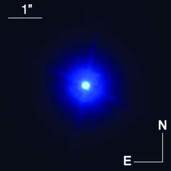
Figure 2: A combined image around K2-105. The image is given in the log color scale. The central region around K2-105 is saturated. This figure shows a 5” $\times$ 5” portion. North is up and East is left.

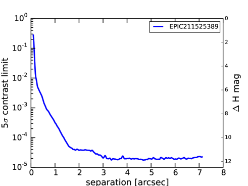
Figure 3: A 5$\sigma$ contrast limit curve around K2-105.

We compute offsets between the central star’s centroids in each frame obtained with and without the ND filter. The reduced images of saturated and unsaturated frames are then offset-corrected, sky-level-subtracted, and combined to produce final deep-integration images. No additional point source which can mimic the observed transit signal is detected in the final image. Hence we compute the detection limit for such sources. The combined saturated image is convolved with the FWHM of the combined unsaturated image, and the standard deviations of counts in annuli segmented from the center of the target are calculated. Aperture photometry for the combined unsaturated image is done to compute the flux count of the target per unit of time. By comparing the flux of the target to the standard deviations of counts in annuli, we create a 5$\sigma$ contrast curve as a function of the separation in arcsec. The combined image of the saturated frames and the 5$\sigma$ contrast curve are shown in Figures 2 and 3. Consequently, we do not find any evidence of contaminants which could mimic the transit signal around K2-105 at the level shown in the contrast curve.

3.3 Joint Transit Light Curve Analysis

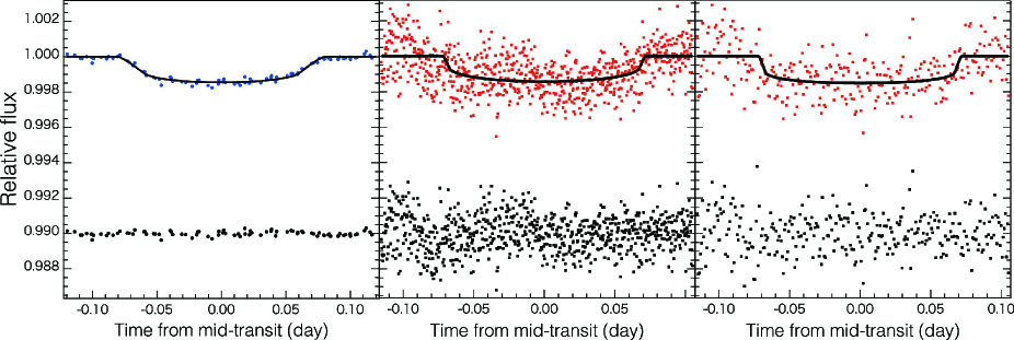
Figure 4: Left panel: The phase-folded, baseline-corrected K2 transit light curve. Blue dots plot the K2 data. A black solid line represents the best-fit transit model that is integrated over the K2 cadence ($\sim 29.4$ minutes). Residuals from the best-fit model are plotted with a vertical offset of $-0.01$. Middle and right panels: Same as the left panel, but the baseline-corrected MuSCAT transit light curves for the $r^{\prime}_{2}$ band (middle) and the $z_{s,2}$ band (right), respectively. Red dots show the MuSCAT data.

We simultaneously fit K2 and MuSCAT transit light curves as follows.

The K2 light curve shown in Figure 1 is separated into nine transit segments, each containing a full-transit (namely, before, during, and after a transit). Note that there is another transit at the beginning of K2 observation, but we exclude this transit since the data before the transit are not available. Each segment includes the data within $\sim 9$ hours from the apparent transit center. We compute the standard deviation of the out-of-transit K2 data, excluding data in the transit segments and apparent outliers (with the excursion larger than 0.001 from the unity). We adopt the standard deviation of the out-of-transit data as an estimate of the uncertainty for each K2 flux value. For K2 transit light curves, we adopt a linear function in time as a baseline model,

$$F_{\rm base}(t) = k_{0}+k_{t}t,$$

where $k_{0}$ is the normalization factor and $k_{t}$ is the coefficient for the time. Other parameters for the K2 transit light curves are the mid-transit time for each transit segment ($T_{c}(E)$, where $E=0$ – 8), and the planet-to-star radius ratio $R_{p}/R_{\star}$ for the K2 bandpass ($K_{p}$).

For the MuSCAT transit light curves, we adopt a novel parametrization for the baseline model to take account for the 2nd-order extinction introduced by Fukui et al. (2016b). As a brief introduction, the parametrization uses the apparent magnitude of the comparison star(s) instead of the airmass, and the baseline function is expressed in magnitudes as follows,

$$m_{t,\mathrm{base}}(t) = k_{0}+k_{t}t+k_{c}m_{c}(t),$$

where $m_{t}$ and $m_{c}$ are the apparent magnitude of the target and comparison star(s), $k_{c}$ is the coefficient for the atmospheric extinction. This parametrization allows us to correct both the airmass extinction and the 2nd-order extinction caused by the different spectral types of comparison stars. See Fukui et al. (2016b) for the mathematical derivation of this method. Other parameters for the MuSCAT transit light curves are the mid-transit time for the MuSCAT observation ($T_{c}(34)$) and $R_{p}/R_{\star}$ for MuSCAT $r^{\prime}_{2}$ and $z_{s,2}$ bands.

Finally, the common planetary transit parameters are the scaled semi-major axis $a/R_{\star}$ and the impact parameter $b$. We place an a priori constraint on $a/Rs$ to be $18.4\pm 2.5$, based on spectroscopically derived $M_{\star}$, $R_{\star}$, and the semi-major axis estimated by Kepler’s third law. We assume an orbital period of $P=8.2672478$ days, which we derive from the K2 transits at the time of identification of the candidate. Although we later derive an improved orbital period, the difference has no impact on fitting results, since we allow all $T_{c}(E)$ to be free parameters.

To estimate the values of the free parameters and their uncertainties, we use a code (Narita et al., 2007) that uses the analytic formula given by Ohta et al. (2009) for the transit light curve model. The analytic transit formula is equivalent to that given by Mandel & Agol (2002) when using the quadratic limb-darkening law. We adopt a methodology for applying priors on limb-darkening described in Fukui et al. (2016a). To reduce a correlation between the quadratic limb-darkening coefficients $u_{1}$ and $u_{2}$, and to appropriately estimate uncertainties for other parameters, we use a combination form of the limb-darkening parametrization $w_{1}=u_{1}\cos(\phi)-u_{2}\sin(\phi)$ and $w_{2}=u_{1}\sin(\phi)+u_{2}\cos(\phi)$, which was introduced by Pál (2008). We adopt $\phi=40^{\circ}$ that is recommended by Pál (2008) and Howarth (2011). We refer the tables of quadratic limb-darkening parameters by Claret et al. (2013) and compute allowed $w_{1}$ and $w_{2}$ values for the stellar parameters presented in Table 1. We employ uniform priors for $w_{1}$ between [0.197, 0.359] for $K_{p}$ band, [0.180, 0.329] for MuSCAT $r^{\prime}_{2}$ band, and [-0.028, 0.191] for MuSCAT $z_{s,2}$ band, respectively. For $w_{2}$, we adopt Gaussian priors as $0.466\pm 0.009$ for $K_{p}$ band, $0.472\pm 0.009$ for MuSCAT $r^{\prime}_{2}$ band, and $0.375\pm 0.011$ for MuSCAT $z_{s,2}$ band, respectively. The priors for the MCMC analysis are summarized in Table 2.

Table 2: Summary of priors for the MCMC analysis.

Parameter	Prior	Explanation
$P$ [days]	8.2672478	Fixed
$a/R_{\star}$	$18.4\pm 2.5$	Added in the penalty function
$w_{1,K_{p}}$	[0.197, 0.359]	Uniform prior
$w_{1,r^{\prime}_{2}}$	[0.180, 0.329]	Uniform prior
$w_{1,K_{p}}$	[-0.028, 0.191]	Uniform prior
$w_{2,K_{p}}$	$0.466\pm 0.009$	Gaussian prior
$w_{2,r^{\prime}_{2}}$	$0.472\pm 0.009$	Gaussian prior
$w_{2,K_{p}}$	$0.375\pm 0.011$	Gaussian prior

Before creating MCMC chains, we first optimize free parameters for each light curve, using the AMOEBA algorithm (Press et al., 1992). The penalty function is given by

$$\chi^{2} = \sum_{\rm K2}\sum_{\rm t}\frac{(f_{\mathrm{obs,t}}-f_{\mathrm{model,t}})^{2}}{\sigma_{\rm f,t}^{2}}$$

$$+ \sum_{\rm MuSCAT}\sum_{\rm t}\frac{(m_{\mathrm{obs,t}}-m_{\mathrm{model,t}})^{2}}{\sigma_{\rm m,t}^{2}}+\frac{(a/R_{\star}-18.4)^{2}}{2.5^{2}},$$

where $f_{\mathrm{obs,t}}$ and $\sigma_{\rm f,t}$ are the relative fluxes of the target in each K2 transit segment and their errors, and $m_{\mathrm{obs,t}}$ and $\sigma_{\rm m,t}$ are the magnitude of the target in $r^{\prime}_{s}$ and $z_{x,2}$ bands and their errors. The model functions $f_{\mathrm{model,t}}$ and $m_{\mathrm{model,t}}$ are combinations of the baseline model and the analytic transit formula mentioned above. We note that the transit model is integrated over the K2 cadence ($\sim 29.4$ minutes) for $f_{\mathrm{model,t}}$. In addition, the time stamps of all data are converted to the $\mathrm{BJD_{TDB}}$ system using the code by Eastman et al. (2010). If the reduced $\chi^{2}$ is larger than unity, we rescale the photometric errors of the data such that the reduced $\chi^{2}$ for each light curve becomes unity. We then estimate the level of time-correlated noise (a.k.a. red noise: Pont et al. (2006)) for each light curve, by calculating the $\beta$ factor introduced by Winn et al. (2008). The $\beta$ factor is used to take into account the time-correlated noise and to properly compensate the possible underestimate of derived uncertainties from analyses of transit photometry. For the purpose, we compute the residuals for each light curve and average the residuals into $M$ bins of $N$ points. We then calculate the actual standard deviation of the binned data $\sigma_{{\rm N,obs}}$ and the ideal standard deviation without any time-correlated noise $\sigma_{{\rm N,ideal}}=\frac{\sigma_{1}}{\sqrt{N}}\sqrt{\frac{M}{M-1}}$, where $\sigma_{1}$ is the standard deviation of the residuals for unbinned data. To account for increased uncertainties due to the time-correlated noise, we compute $\beta=\sigma_{{\rm N,obs}}/\sigma_{{\rm N,ideal}}$ for various $N$. If $\beta$ is significantly higher than unity, it implies the presence of the time-correlated noise. Consequently, we find no significant time-correlated noise in K2 light curves, while MuSCAT light curves show significant time-correlated noise, especially in the $r^{\prime}_{2}$ band. We adopt $\beta=1.56409$ for the $r^{\prime}_{2}$ band and $\beta=1.08181$ for the $z_{s,2}$ band, which are the median values of $\beta$ for $N=$ 5–20 binning cases in each band, and further rescale the errors of the light curves by multiplying them by their $\beta$ factors.

Finally, we employ the Markov Chain Monte Carlo (MCMC) code (Narita et al., 2013; Fukui et al., 2016a) to compute the posterior distributions for the free parameters. We create 3 chains of 12,000,000 points, and discard the first 2,000,000 points from each chain as “burn-in”. The jump sizes of parameters in each MCMC step are adjusted such that acceptance ratios become $\sim$23%, which is considered as an optimal acceptance ratio for efficient convergence of MCMC (see e.g., Ford (2005)).

Table 3 presents the median values and uncertainties, which are defined by the 15.87 and 84.13 percentile levels of the merged posterior distributions. The baseline corrected transit light curves (in flux) are plotted in Figure 4. We find that $R_{p}/R_{\star}$ for all three bands are consistent with one another and that the MuSCAT light curves are consistent with a flat-bottomed transit. To derive the orbital ephemeris we fit a linear model to the mid-transit times, yielding a period of $P=8.2669016\pm 0.0000581$ days and a time of first transit of $T_{c}(0)=2457147.99107\pm 0.00098$ (BJD_TDB), with $\chi^{2}$ of 11.499 for 8 degrees of freedom. Note that in this fit we adopt the larger-side uncertainty if uncertainties of respective mid-transit times are asymmetric. To be conservative, we rescale the uncertainties of $P$ and $T_{c}(0)$ by $\sqrt{11.499/8}$, and the rescaled uncertainties are presented in Table 3. This refined ephemeris will be useful for future transit observations of K2-105 b.

Table 3: Planetary Parameters of K2-105 b

Parameter	Value
(MCMC Parameters)
$a/R_{\star}$	$17.96_{-2.34}^{+0.91}$
$b$	$0.328_{-0.225}^{+0.249}$
$R_{p}/R_{\star}$ [$K_{p}$ band]	$0.03472_{-0.00067}^{+0.00133}$
$R_{p}/R_{\star}$ [$r^{\prime}_{2}$ band]	$0.03444_{-0.00421}^{+0.00445}$
$R_{p}/R_{\star}$ [$z_{s,2}$ band]	$0.03651_{-0.00541}^{+0.00388}$
$T_{c}(0)$ [BJD - 2450000]	$7147.98960_{-0.00371}^{+0.00441}$
$T_{c}(1)$ [BJD - 2450000]	$7156.25371_{-0.00209}^{+0.00206}$
$T_{c}(2)$ [BJD - 2450000]	$7164.52415_{-0.00224}^{+0.00221}$
$T_{c}(3)$ [BJD - 2450000]	$7172.79050_{-0.00199}^{+0.00213}$
$T_{c}(4)$ [BJD - 2450000]	$7181.06464\pm 0.00244$
$T_{c}(5)$ [BJD - 2450000]	$7189.32677_{-0.00212}^{+0.00202}$
$T_{c}(6)$ [BJD - 2450000]	$7197.59274_{-0.00294}^{+0.00287}$
$T_{c}(7)$ [BJD - 2450000]	$7205.86050_{-0.00197}^{+0.00201}$
$T_{c}(8)$ [BJD - 2450000]	$7214.12742_{-0.00343}^{+0.00392}$
$T_{c}(34)$ [BJD - 2450000]	$7429.06529_{-0.00157}^{+0.00142}$
$K$ [m s-1]	$9.4\pm 5.8$ ($<$26.8 )
(Derived Parameters)
$P$ [days]	$8.266902\pm 0.000070$
$T_{c}(0)$ † [BJD - 2450000]	$7147.99107\pm 0.00117$
$R_{p}$ [$R_{\oplus}$]	$3.59_{-0.39}^{+0.44}$
$R_{p}$ [$R_{Jup}$]	$0.369_{-0.034}^{+0.039}$
$i$ [∘]	$88.95_{-1.07}^{+0.73}$
$T_{14}$ [days]	$0.14426_{-0.00203}^{+0.00224}$
$M_{p}$ [$M_{\oplus}$]	$30\pm 19$ ($<$90 )

An upper limit at 99.865 percentile (3$\sigma$) level. This is the origin for the transit ephemeris. Based on $R_{p}/R_{\star}$ in $K_{p}$ band.

3.4 Subaru/HDS Radial Velocities and a Mass Upper Limit

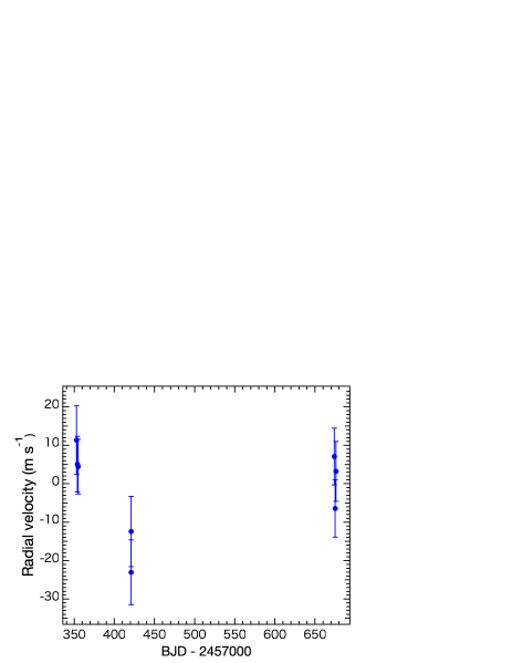
Figure 5: Relative radial velocities (blue points) of K2-105 taken with the Subaru HDS.

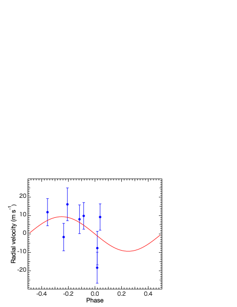
Figure 6: Radial velocities (blue points) phased by the orbital period given in Table 3 and the best-fit RV model (red line).

We employ the RV pipeline for the Subaru HDS described in Sato et al. (2002) to extract the relative RVs with respect to the template iodine-free spectrum. The derived RVs are presented in Table 4 and plotted in Figure 5. We do not find any significant long-term radial velocity drift.

To model the observed RVs, we adopt an RV model, $v_{\mathrm{model}}=-K\sin\phi+\gamma$, where $K$, $\phi$, $\gamma$ are the RV semi-amplitude, the orbital phase relative to the mid-transit, and the offset RV relative to the template spectrum. We fix the orbital period $P$ to 8.2669016 days and the origin of the transit ephemeris $T_{c}(0)$ to 2457147.99107 (BJD_TDB) as derived in §3.3. We do not consider the Rossiter-McLaughlin effect, since there is no RV data during a transit. We also neglect the eccentricity $e$, since it is indeterminable with the current RVs.

We first optimize $K$ and $\gamma$ using the AMOEBA algorithm (Press et al., 1992), and create an MCMC chain of 500,000 points starting from the optimal parameters. The acceptance ratio is set to $\sim$23%. The phased RVs and the best-fit RV model are shown in Figure 6. The median values and uncertainties of the free parameters are presented in Table 3. We also present a 3$\sigma$ upper limit (99.865 percentile level) of $K$ in Table 3. Consequently, the RV semi-amplitude is $9.4\pm 5.8$ m s^-1, which corresponds to $30\pm 19$ M_⊕ for the mass of K2-105 b. At this point, the current RVs are not sufficient to determine the RV semi-amplitude and the mass of K2-105 b precisely. Nevertheless, we can put a constraint on $K<26.8$ m s^-1 at the 3$\sigma$ level, which corresponds to a mass upper limit of $90M_{\oplus}$ or $0.00027M_{\odot}$. This upper limit ensures that the mass of K2-105 b is within a planetary mass, excluding the possibility of an eclipsing binary scenario for this system.

Table 4: Radial velocities of K2-105 taken with Subaru/HDS.

BJDTDB	Value [m s-1]	Error [m s-1]
2457352.95525	11.33	8.92
2457353.96869	5.08	7.25
2457354.98800	4.45	7.14
2457420.93976	-23.06	8.42
2457420.94741	-12.43	9.14
2457674.12841	7.07	7.38
2457675.13374	-6.44	7.45
2457676.11418	3.23	7.80

4 Discussions

4.1 Confirmation of the Planetary Nature of K2-105 b

To further validate the planetary nature of the transit signal, we use the open-source Python code vespa (Morton, 2012, 2015), which employs a robust statistical framework to calculate the False Positive Probability (FPP) of the transit signal. It does this by taking into account a variety of factors: the size of the photometric aperture of K2, the source density along the line of sight as determined from galaxy simulations, constraints on contaminants from high resolution imaging contrast curves, physical properties of the host star from spectroscopically-derived parameters and broadband photometry, and comparisons of the shape of the phase-folded K2 light curve to a large number of realistic false positive scenarios.

We input our results presented in the last section to vespa and find the final FPP for this target to be extremely low ($<10^{-6}$), which strongly indicates a planetary nature for the origin of the observed transit signals. We therefore rule out all of the false positive scenarios accounted for by vespa (i.e. hierarchical triple systems, eclipsing binaries, blended background eclipsing binaries).

We conclude that K2-105 b is a bona fide planet, based on the mass constraint presented in §3.4 and the extremely low FPP.

4.2 The New Transit Ephemeris and a Hint of Transit Timing Variation

We have derived the new transit ephemeris for K2-105 b as $P=8.266902\pm 0.000070$ days and $T_{c}(0)=2457147.99107\pm 0.00117$ in BJD_TDB. This is indeed the first reliable transit ephemeris for K2-105 b, since Pope et al. (2016) and Barros et al. (2016), who reported EPIC 211525389 b as a candidate planet, presented a transit ephemeris without any uncertainty. Using the transit ephemeris we have derived from our observations, transits of K2-105 b in 2017 can be predicted with uncertainties of only about 10 minutes, which will facilitate the scheduling of future transit observations.

We check the possible presence of transit timing variation (TTV) for the transits of K2-105 b. Figure 7 plots residuals of the observed mid-transit times from the current transit ephemeris. While if only K2 transits are taken into account, a linear fit to the mid-transit times gives $P=8.2675710\pm 0.0003569$ days and $T_{c}(0)=2457147.98853\pm 0.00164$ in BJD_TDB, with $\chi^{2}$ of 7.884 for 7 degree-of-freedom. The transit for the MuSCAT run occurred about 30 min earlier than the prediction from the K2-only transits, although the difference is at the 2$\sigma$ level. The discrepancy is statistically not significant, but it may suggest that an additional non-transiting planet exist as is the case for K2-19 b & c (e.g., Armstrong et al. (2015); Narita et al. (2015a)). Alternatively, stellar activities such as star spots may play a role in the apparent discrepancy (see e.g., Oshagh et al. (2013)). To confirm the presence of TTVs for K2-105 b, further transit monitoring is needed.

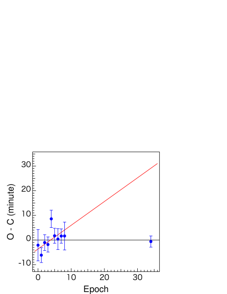
Figure 7: Residuals of the observed mid-transit times from the current best-fit transit ephemeris. The red line represents the best-fit transit ephemeris for the transits from K2 only. We note that the transit ephemeris from K2 has an uncertainty of $\sim$17 minutes at the epoch of 34. Thus the discrepancy is still within the 2$\sigma$ level.

4.3 K2-105 b in the Context of Period-Radius and Mass-Radius Relation

Occurrence rates of planets derived from RV surveys and the Kepler indicate that short-period Neptune-sized planets such as K2-105 b are only rarely found in planetary systems around solar-type stars (e.g., Howard et al. (2012); Petigura et al. (2013)). Figure 8 shows an orbital period–radius distribution of transiting planets with $P\leq 50$ days. We see a clear lack of planets with radii of $\sim 3.5-10\,R_{\oplus}$ around solar-type stars, albeit interestingly, no hot Jupiter with radius of $\gtrsim 10\,R_{\oplus}$ is seen around stars with $M_{\star}\leq 0.45\,M_{\odot}$. These features, also pointed out by previous studies (e.g., Mazeh et al. (2016); Matsakos & Königl (2016)), may reflect a size boundary between a failed core and a gas giant, which corresponds to a critical core mass that triggers gas accretion in a runaway fashion, or mass loss via photo-evaporation. The latter case can be a useful indicator to evaluate the efficiency of atmospheric escape due to a stellar irradiation or injection of high-energy particles. Thus, the discovery of K2-105 b can be an interesting benchmark to disentangle the origin of Neptune-sized planets close to central stars.

Figure 9 shows theoretical mass-radius relations for three types of planets and transiting exoplanets with known mass. We find that K2-105 b is not a bare rocky planet but likely has an atmosphere ($<$ 10% of its total mass) if its total mass is smaller than $30\,M_{\oplus}$. K2-105 b orbits at $a_{\rm p}=0.081\pm 0.006$ AU around a G-dwarf with the mass of $1.01\pm 0.07\,M_{\odot}$. According to Owen & Wu (2013), K2-105 b can retain its atmosphere under an intense stellar X-ray and EUV irradiation during an estimated stellar age of older than 0.6 Gyr, if the core mass is greater than $\sim 6\,M_{\oplus}$.

If K2-105 b is a gas dwarf, how did it form? There are two possible formation scenarios, namely, in-situ gas accretion onto a massive core (Ikoma & Hori, 2012; Lee et al., 2014; Ormel et al., 2015) or inward migration of a Neptune-like planet (e.g., Bodenheimer & Lissauer (2014)). However, we cannot rule out both stories because of an unknown mass of K2-105 b. Thus, mass determination from follow-up RV observations will be indispensable for constraining the formation history and quantifying the effect of photo-evaporation.

In addition, close-in Neptune-sized planets as represented by K2-105 b would be suggestive of uncovering how the Solar System was born. There is no K2-105 b-like planet in the Solar System, instead the two ice giants orbit beyond $\sim$20 AU. As one possibility, this might be caused by the presence of Jupiter and Saturn orbiting within the orbits of the two ice giants, acting as a barrier against inward migrating cores. Long-term RV monitoring of K2-105 to constrain the possibility of outer giant planets should be helpful in understanding the orbital evolutions of Neptune-like planets and the Solar System. Therefore, long-term RV monitoring of this system would be also encouraged.

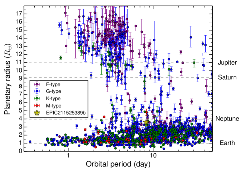
Figure 8: Period-radius relation of confirmed transiting exoplanets with $P\leq 50$ days around F-type ($M_{\star}=1.04-1.4\,M_{\odot}$), G-type ($M_{\star}=0.8-1.04\,M_{\odot}$), K-type ($M_{\star}=0.45-0.8\,M_{\odot}$), and M-type stars ($M_{\star}=0.08-0.45\,M_{\odot}$) as of 2016 August; the data come from http://exoplanet.eu. Planets for which the radius uncertainty exceeds 20% of their representative values are excluded.

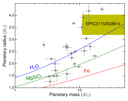
Figure 9: Mass-radius relation of confirmed transiting exoplanets as of 2016 September; the data come from http://exoplanet.eu. Planets with uncertainties in mass and radius over 20% of their representative values are not shown here. Theoretical models of iron, water, and silicate planets are based on Zeng & Sasselov (2013). We adopt the possible range of K2-105 b’s mass derived from RV measurements by the Subaru HDS, $M_{\rm p}=30\pm 19\,M_{\oplus}$ and its radius of $R_{\rm p}=3.59^{+0.44}_{-0.39}\,R_{\oplus}$.

5 Summary

We have confirmed the planetary nature of K2-105 b, using transit photometry from the K2 mission, high dispersion spectroscopy and RVs from Subaru/HDS, high-contrast AO imaging from Subaru/HiCIAO, and ground-based transit photometry from Okayama/MuSCAT. The host star K2-105 is located in K2 campaign field 5, and estimated to be a metal-rich G-dwarf. Although further RV monitoring is required to precisely determine the mass of K2-105 b, the Subaru HDS RVs put a stringent constraint on the mass of K2-105 b as less than 90$M_{\oplus}$ or $0.00027M_{\odot}$ at the 3$\sigma$ level, ensuring that the mass of K2-105 b is well within the planetary mass range. Our joint analysis of the transit data from K2 and MuSCAT yields an orbital period of $P=8.266902\pm 0.000070$ days and an origin of mid-transit time $T_{c}(0)=2457147.99107\pm 0.00117$ in BJD_TDB. The transit ephemeris is accurate enough to predict transit times of K2-105 b with uncertainties of less than 20 minutes for the next few years. We have found that the transit observed with the Okayama/MuSCAT occurred about 30 minutes earlier than the prediction from the K2-only transits. Although the discrepancy from the prediction is statistically marginal at the 2$\sigma$ level, this may suggest that additional long period or non-transiting planet(s) exist in the system, which increases the need for further transit and RV measurements of this system.

The transit depth of K2-105 b, $R_{p}/R_{\star}\sim 0.035$, corresponds to a planetary radius of $R_{p}=3.59_{-0.39}^{+0.44}$ $R_{\oplus}$. Thus K2-105 b is a short-period Neptune-sized planet. As K2-105 b is a transiting planet around a relatively bright host star, it is a favorable and important target for characterization of its mass via RV measurements, its atmosphere via transmission spectroscopy, spin-orbit (mis)alignment via the Rossiter-McLaughlin effect or doppler tomography, and the presence of additional planet via TTVs and/or RV trends. Such further characterization will be vital for understanding the formation and migration history of this planetary system.

6 Funding

This work was supported by Japan Society for Promotion of Science (JSPS) KAKENHI Grant Numbers JP25247026, JP16K17660, 25-8826, JP16K17671, and JP15H02063. This work was also supported by the Astrobiology Center Project of National Institutes of Natural Sciences (NINS) (Grant Numbers AB271009, AB281012 and JY280092). I.R. acknowledges support by the Spanish Ministry of Economy and Competitiveness (MINECO) through grant ESP2014-57495-C2-2-R.

We acknowledge Roberto Sanchis-Ojeda, who established the ESPRINT collaboration. We thank supports by Akito Tajitsu and Hikaru Nagumo for our Subaru HDS observation, Jun Hashimoto for Subaru HiCIAO observation, and Timothy Brandt for HiCIAO data reduction. This paper is based on data collected at the Subaru telescope and Okayama 188cm telescope, which are operated by the National Astronomical Observatory of Japan. The data analysis was in part carried out on common use data analysis computer system at the Astronomy Data Center, ADC, of the National Astronomical Observatory of Japan. PyFITS and PyRAF were useful for our data reductions. PyFITS and PyRAF are products of the Space Telescope Science Institute, which is operated by AURA for NASA. Our analysis is also based on observations made with the NASA/ESA Hubble Space Telescope, and obtained from the Hubble Legacy Archive, which is a collaboration between the Space Telescope Science Institute, the Space Telescope European Coordinating Facility (ST-ECF/ESA) and the Canadian Astronomy Data Centre (CADC/NRC/CSA). This work has made use of data from the European Space Agency (ESA) mission Gaia (http://www.cosmos.esa.int/gaia), processed by the Gaia Data Processing and Analysis Consortium (DPAC, http://www.cosmos.esa.int/web/gaia/dpac/consortium). Funding for the DPAC has been provided by national institutions, in particular the institutions participating in the Gaia Multilateral Agreement. We acknowledge the very significant cultural role and reverence that the summit of Mauna Kea has always had within the indigenous people in Hawai’i.

References

- Adibekyan et al. (2013) Adibekyan, V. Z., et al. 2013, A&A, 560, A51
- Armstrong et al. (2015) Armstrong, D. J., et al. 2015, A&A, 582, A33
- Barros et al. (2016) Barros, S. C. C., Demangeon, O., & Deleuil, M. 2016, ArXiv e-prints, arXiv:1607.02339
- Beaugé & Nesvorný (2013) Beaugé, C., & Nesvorný, D. 2013, ApJ, 763, 12
- Bodenheimer & Lissauer (2014) Bodenheimer, P., & Lissauer, J. J. 2014, ApJ, 791, 103
- Brandt et al. (2013) Brandt, T. D., et al. 2013, ApJ, 764, 183
- Bruntt et al. (2010) Bruntt, H., et al. 2010, MNRAS, 405, 1907
- Claret et al. (2013) Claret, A., Hauschildt, P. H., & Witte, S. 2013, A&A, 552, A16
- Crossfield et al. (2015) Crossfield, I. J. M., et al. 2015, ApJ, 804, 10
- Crossfield et al. (2016) Crossfield, I. J. M., et al. 2016, ApJS, 226, 7
- Dai et al. (2016) Dai, F., et al. 2016, ApJ, 823, 115
- Dotter et al. (2008) Dotter, A., Chaboyer, B., Jevremović, D., Kostov, V., Baron, E., & Ferguson, J. W. 2008, ApJS, 178, 89
- Eastman et al. (2010) Eastman, J., Siverd, R., & Gaudi, B. S. 2010, PASP, 122, 935
- Ford (2005) Ford, E. B. 2005, AJ, 129, 1706
- Fukui et al. (2011) Fukui, A., et al. 2011, PASJ, 63, 287
- Fukui et al. (2016a) Fukui, A., et al. 2016a, ApJ, 819, 27
- Fukui et al. (2016b) Fukui, A., Livingston, J., Narita, N., Hirano, T., Onitsuka, M., Ryu, T., & Kusakabe, N. 2016b, ArXiv e-prints, arXiv:1610.01333
- Gaia Collaboration (2016) Gaia Collaboration. 2016, ArXiv e-prints, arXiv:1609.04153
- Gray (2005) Gray, D. F. 2005, The Observation and Analysis of Stellar Photospheres (UK: Cambridge University Press, 2005)
- Hayano et al. (2008) Hayano, Y., et al. 2008, in Presented at the Society of Photo-Optical Instrumentation Engineers (SPIE) Conference, Vol. 7015, Society of Photo-Optical Instrumentation Engineers (SPIE) Conference Series
- Helled et al. (2016) Helled, R., Lozovsky, M., & Zucker, S. 2016, MNRAS, 455, L96
- Hirano et al. (2012) Hirano, T., Sanchis-Ojeda, R., Takeda, Y., Narita, N., Winn, J. N., Taruya, A., & Suto, Y. 2012, ApJ, 756, 66
- Hirano et al. (2014) Hirano, T., Sanchis-Ojeda, R., Takeda, Y., Winn, J. N., Narita, N., & Takahashi, Y. H. 2014, ApJ, 783, 9
- Hirano et al. (2016a) Hirano, T., et al. 2016a, ApJ, 820, 41
- Hirano et al. (2016b) Hirano, T., et al. 2016b, ApJ, 825, 53
- Howard et al. (2012) Howard, A. W., et al. 2012, ApJS, 201, 15
- Howarth (2011) Howarth, I. D. 2011, MNRAS, 418, 1165
- Howell et al. (2014) Howell, S. B., et al. 2014, PASP, 126, 398
- Huber et al. (2016) Huber, D., et al. 2016, ApJS, 224, 2
- Ikoma & Hori (2012) Ikoma, M., & Hori, Y. 2012, ApJ, 753, 66
- Jenkins et al. (2010) Jenkins, J. M., et al. 2010, ApJ, 713, L87
- Kovács et al. (2002) Kovács, G., Zucker, S., & Mazeh, T. 2002, A&A, 391, 369
- Kurucz (1993) Kurucz, R. 1993, ATLAS9 Stellar Atmosphere Programs and 2 km/s grid. Kurucz CD-ROM No. 13. Cambridge, Mass.: Smithsonian Astrophysical Observatory, 1993., 13
- Lee et al. (2014) Lee, E. J., Chiang, E., & Ormel, C. W. 2014, ApJ, 797, 95
- Lillo-Box et al. (2016) Lillo-Box, J., et al. 2016, ArXiv e-prints, arXiv:1601.07635
- Lindegren et al. (2016) Lindegren, L., et al. 2016, ArXiv e-prints, arXiv:1609.04303
- Mandel & Agol (2002) Mandel, K., & Agol, E. 2002, ApJ, 580, L171
- Mann et al. (2016) Mann, A. W., et al. 2016, ApJ, 818, 46
- Matsakos & Königl (2016) Matsakos, T., & Königl, A. 2016, ApJ, 820, L8
- Mazeh et al. (2016) Mazeh, T., Holczer, T., & Faigler, S. 2016, A&A, 589, A75
- Morton (2012) Morton, T. D. 2012, ApJ, 761, 6
- Morton (2015) Morton, T. D. 2015, VESPA: False positive probabilities calculator, Astrophysics Source Code Library
- Narita et al. (2007) Narita, N., et al. 2007, PASJ, 59, 763
- Narita et al. (2013) Narita, N., et al. 2013, ApJ, 773, 144
- Narita et al. (2015a) Narita, N., et al. 2015a, ApJ, 815, 47
- Narita et al. (2015b) Narita, N., et al. 2015b, Journal of Astronomical Telescopes, Instruments, and Systems, 1, 045001
- Noguchi et al. (2002) Noguchi, K., et al. 2002, PASJ, 54, 855
- Ofir (2014) Ofir, A. 2014, A&A, 561, A138
- Ohta et al. (2009) Ohta, Y., Taruya, A., & Suto, Y. 2009, ApJ, 690, 1
- Ormel et al. (2015) Ormel, C. W., Shi, J.-M., & Kuiper, R. 2015, MNRAS, 447, 3512
- Oshagh et al. (2013) Oshagh, M., Santos, N. C., Boisse, I., Boué, G., Montalto, M., Dumusque, X., & Haghighipour, N. 2013, A&A, 556, A19
- Owen & Wu (2013) Owen, J. E., & Wu, Y. 2013, ApJ, 775, 105
- Pál (2008) Pál, A. 2008, MNRAS, 390, 281
- Petigura et al. (2013) Petigura, E. A., Howard, A. W., & Marcy, G. W. 2013, Proceedings of the National Academy of Science, 110, 19273
- Pont et al. (2006) Pont, F., Zucker, S., & Queloz, D. 2006, MNRAS, 373, 231
- Pope et al. (2016) Pope, B. J. S., Parviainen, H., & Aigrain, S. 2016, MNRAS, 461, 3399
- Press et al. (1992) Press, W. H., Teukolsky, S. A., Vetterling, W. T., & Flannery, B. P. 1992, Numerical recipes in C. The art of scientific computing (Cambridge: University Press, —c1992, 2nd ed.)
- Sanchis-Ojeda et al. (2015) Sanchis-Ojeda, R., et al. 2015, ApJ, 812, 112
- Sato et al. (2002) Sato, B., Kambe, E., Takeda, Y., Izumiura, H., & Ando, H. 2002, PASJ, 54, 873
- Skrutskie et al. (2006) Skrutskie, M. F., et al. 2006, AJ, 131, 1163
- Suzuki et al. (2010) Suzuki, R., et al. 2010, in Society of Photo-Optical Instrumentation Engineers (SPIE) Conference Series, Vol. 7735, Society of Photo-Optical Instrumentation Engineers (SPIE) Conference Series, 30
- Tajitsu et al. (2012) Tajitsu, A., Aoki, W., & Yamamuro, T. 2012, PASJ, 64, 77
- Takeda et al. (2002) Takeda, Y., Ohkubo, M., & Sadakane, K. 2002, PASJ, 54, 451
- Takeda et al. (2005) Takeda, Y., Ohkubo, M., Sato, B., Kambe, E., & Sadakane, K. 2005, PASJ, 57, 27
- Tamura et al. (2006) Tamura, M., et al. 2006, in Presented at the Society of Photo-Optical Instrumentation Engineers (SPIE) Conference, Vol. 6269, Ground-based and Airborne Instrumentation for Astronomy. Edited by McLean, Ian S.; Iye, Masanori. Proceedings of the SPIE, Volume 6269, pp. 62690V (2006).
- Torres et al. (2010) Torres, G., Andersen, J., & Giménez, A. 2010, A&A Rev., 18, 67
- Van Eylen et al. (2016a) Van Eylen, V., et al. 2016a, ApJ, 820, 56
- Van Eylen et al. (2016b) Van Eylen, V., et al. 2016b, ArXiv e-prints, arXiv:1605.09180
- Winn et al. (2008) Winn, J. N., et al. 2008, ApJ, 683, 1076
- Yi et al. (2001) Yi, S., Demarque, P., Kim, Y.-C., Lee, Y.-W., Ree, C. H., Lejeune, T., & Barnes, S. 2001, ApJS, 136, 417
- Zeng & Sasselov (2013) Zeng, L., & Sasselov, D. 2013, PASP, 125, 227