Approximate Value Iteration for Risk-aware Markov Decision Processes

Abstract

We consider large-scale Markov decision processes (MDPs) with a risk measure of variability in cost, under the risk-aware MDPs paradigm. Previous studies showed that risk-aware MDPs, based on a minimax approach to handling risk, can be solved using dynamic programming for small to medium sized problems. However, due to the “curse of dimensionality”, MDPs that model real-life problems are typically prohibitively large for such approach. In this paper, we employ an approximate dynamic programming approach, and develop a family of simulation-based algorithms to approximately solve large-scale risk-aware MDPs. In parallel, we develop a unified convergence analysis technique to derive sample complexity bounds for this new family of algorithms.

I Introduction

Markov decision processes (MDPs) (e.g., [1, 2]) are a well established framework for modeling sequential decision-making problems. They have been studied and applied extensively. The classical MDPs search for a policy with minimum expected cost. Nonetheless, it turns out that solely considering the expectation is insufficient in various applications (see the motivated example in [3]). In particular, the expected value can fail to be useful when there is significant stochasticity in the MDP transitions, which may lead to significant variability in the cost distribution [4].

The natural method for dealing with stochasticity, motivated by classical studies in the financial literature, is through the notion of risk, such as its exponential-utility [4], variance [5], or conditional value-at-risk (CVaR) [6]. Such measures capture the variability of the cost, or quantify the effect of rare but potentially disastrous outcomes. The risk measure is extended to the setting of sequential optimization problems (e.g., [4, 7]), in which the objective is to minimize a risk measure defined over the whole time horizon. In this setting, the total cost is considered as a standard random variable, without any regard to the temporal nature of the process generating it. In particular, expected utility minimizing MDPs are considered earlier in [8]. MDPs with variance-related criteria are studied in [9], while CVaR minimizing MDPs are explored in [10]. It was shown that problems of this type can be difficult [11], and even for the mean-variance model the Bellman’s principle of optimality does not hold and the associated MDPs are NP-hard [12]. Moreover, these problems may lead to “time inconsistent” phenomenon, i.e., the analysis of risk in a multi-period setting can be a treacherous exercise as identical risk preferences can imply vastly different decisions at different time periods [13]. To resolve the issues of these models, time-consistent Markov risk measures were proposed in [3]. The concept of time consistency (e.g., [14]) is usually defined as follows: if a certain outcome is considered less risky in all states of the world at stage $t+1$, then it should also be considered less risky at stage $t$. Markov risk measures capture the multi-period nature of the decision-making process in the definition of the risk, and can be written as compositions of one-step conditional risk measures (these are simply risk measures defined in a conditional setting, analogous to the conditional expectation for the traditional case). In addition, Markov risk measures are notable because they readily yield minimax formulation and the corresponding optimal solution can be obtained using dynamic programming (DP) [3], at least for small to medium sized MDPs. Broadly speaking, the risk-aware dynamic programming is useful in settings with either heavy-tailed distributions or rare high-impact events. For example, heavy-tailed distributions arise frequently in finance (e.g., [15, 16]) as well as energy and sustainability [17]; rare high-impact events may appear in inventory problems [18] as well as management of high-value assets [19].

This paper considers planning in large risk-aware MDPs with Markov risk measures. It is widely known that, due to the “curse of dimensionality,” practical problems modeled as MDPs often have prohibitively large state spaces, under which the previous work [3] with exact DP approach becomes intractable. Many approximation schemes have been proposed to alleviate the curse of dimensionality of large-scale risk-neutral MDPs, among which approximate dynamic programming (ADP) is a popular approach and has been used successfully in large-scale problems with hundreds of state dimensions [20]. Simulation-based algorithms, algorithms which randomly sample the MDP state space and simulate MDP trajectories, comprise a large part of the work on ADP. They have been shown to give good solutions with high probability for classical MDPs (e.g., [21, 22, 23, 24]).

There is considerable development of simulation-based algorithms for risk-aware MDPs with Markov risk measures in the literature, but the computational and theoretical challenges have not been explored as thoroughly. Specifically, the recent work [17] proposes a simulation-based ADP algorithm for risk-aware MDPs. However, it has limited use since it only considers a specific choice of Markov risk measures called dynamic quantile-based risk measures. A cutting plane algorithm for time-consistent multistage linear stochastic programming problems is given in [25], but restricted to finite decision horizons. In [26], an actor-critic style sampling-based algorithm for Markov risk is developed. Although the sensitivity of approximation error is analyzed, the algorithm can only search for a locally optimal policy. Risk-averse dual dynamic programming is introduced in [27] for MDPs with hybrid continuous-discrete state space. Even though the method yields an output that converges to the optimal solution, the significant weaknesses are that it requires the linearity of state and action spaces, and the convergence criterion is not well defined. Our goal in this paper is to consider the whole class of Markov risk measures, propose a new simulation-based ADP approach, and develop improved convergence results and error bounds.

Our first contribution is a new family of computationally tractable and simulation-based algorithms for risk-aware MDPs with infinite state space. We show how to develop risk-aware analogs of several major simulation-based algorithms for classical MDPs (e.g., [28, 22]), which cannot optimize Markov risk measures. In particular, the main novelty of our proposed algorithms is twofold. First, not all existing ADP techniques for classical MDPs are proper for the risk-aware setting. A typical example is the approximate linear programming approach [21] which yields a non-convex formulation in our setting. Second, the empirical estimation of risk is more complex than the empirical estimation of expectation in classical ADP algorithms (e.g., [22, 24]). We use extensive numerical experiments to verify the validity and effectiveness of our proposed algorithms for risk-aware MDPs. To the best of our knowledge, it is the first time approximate value iteration has been proposed for Markov risk measures in the risk-aware MDPs literature.

The second contribution of the paper is a unified convergence and sample complexity analysis technique that applies to a broad family of algorithms, including all of the algorithms considered in this paper. The technique is inspired by the existing convergence analysis for classical MDPs such as weighted $p-$norm performance bounds[22], supremum norm analysis[28] and stochastic dominance framework[24]. Yet, we must extend the existing convergence analysis to the minimax setting, which covers risk-aware MDPs. The critical difference in our approach is that in the risk-aware setting, we have the added difficulty in bounding approximation errors in both each and final iterations due to the minimax DP formulation.

This paper is organized as follows. In Section II we review necessary preliminaries for classical and risk-aware MDPs. Next, in Section III we propose and discuss a general family of simulation-based algorithms for risk-aware MDPs and report their convergence results. Section IV then focuses on the key issue of empirical estimation of risk functions, which plays a major role in all of our algorithms. Section V offers an alternative convergence analysis based on the technique in [24]. In the following Section VI we present the proofs of all of our main results. Section VII reports numerical experiments that serve to illustrate the methods in this paper, and we conclude in Section VIII. Proofs of all technical results can be found in the Appendix.

II Preliminaries

This section reviews important preliminary concepts for both classical and risk-aware MDPs.

II-A Classical MDP

A discounted MDP is defined as a 5-tuple $\left(\mathbb{S},\mathbb{A},P,c,\gamma\right),$ where $\mathbb{S}$ and $\mathbb{A}$ are the state and action space, $P(\cdot|s,a)$ is the transition probability distribution, $c(s,a)$ is a bounded, deterministic, and state-action dependent cost, and $0<\gamma<1$ is a discount factor. In this paper, we consider continuous state space, finite action MDPs (i.e., the cardinality $|\mathbb{A}|<+\infty$). For the sake of simplicity, we assume that $\mathbb{S}$ is a bounded, closed subset of a Euclidean space $\mathbb{R}^{d}$. Let $\mathbb{K}\triangleq\mathbb{S}\times\mathbb{A}$ denote the set of all state-action pairs. We make the following assumption on the cost function $c$ throughout this paper.

Assumption 1

$0\leq c(s,a)\leq c_{\max}<+\infty$ for all $\left(s,a\right)\in\mathbb{K}$.

Let $J_{\max}\triangleq c_{\max}/\left(1-\gamma\right)$. We denote the space of bounded measurable functions with domain $\mathbb{S}$ as $B(\mathbb{S})$ and the space of measurable functions $f\mbox{ : }\mathbb{S}\rightarrow\mathbb{R}$ bounded by $J_{\max}$ as $B\left(\mathbb{S};J_{\max}\right)$. Let $\mathcal{B}(\mathbb{S})$ be a Borel $\sigma-$algebra and $\mathcal{P}\left(\mathbb{S}\right)$ be the space of probability measures over $\mathbb{S}$ w.r.t. $\mathcal{B}\left(\mathbb{S}\right)$. For a probability measure $\mu\mathcal{\in P\left(\mathbb{S}\right)}$ and $1\leq p<+\infty$, we let $\mathcal{L}_{p}(\mathbb{S},\mathcal{B}\left(\mathbb{S}\right),\mu)$ be the space of measurable mappings $f\mbox{ : }\mathbb{S}\rightarrow\mathbb{R}$ such that $\|f\|_{p,\mu}\triangleq(\int|f\left(s\right)|^{p}\mu\left(ds\right))^{1/p}<+\infty$. Furthermore, we denote by $\Pi$ the class of stationary deterministic Markov policies: mappings $\pi\mbox{ : }\mathbb{S}\rightarrow\mathbb{A}$ which only depend on history through the current state. We only consider such policies since it is well known that there is an optimal policy within this class for classical MDPs [1]. For a given state $s\in\mathbb{S}$, $\pi\left(s\right)\in\mathbb{A}$ is the action chosen in state $s$ under the policy $\pi$. The deterministic stationary policy $\pi$ defines the transition probability kernel $P^{\pi}$ according to $P^{\pi}\left(dy|s\right)=P\left(dy|s,\pi\left(s\right)\right)$. We define two operators related to $P^{\pi}$. The right-linear operator $P^{\pi}\left(\cdot\right)\mbox{ : }B(\mathbb{S})\rightarrow B(\mathbb{S})$ is defined as $\left(P^{\pi}J\right)\left(s\right)=\int J\left(y\right)P^{\pi}\left(dy|s\right),$ where $J\in B\left(\mathbb{S}\right),$ and the left-linear operator $\left(\cdot\right)P^{\pi}:\mathcal{P}\left(\mathbb{S}\right)\rightarrow\mathcal{P}\left(\mathbb{S}\right)$ is defined as $\left(\mu P^{\pi}\right)\left(dy\right)=\int P^{\pi}\left(dy|s\right)\mu\left(ds\right),$ where $\mu\in\mathcal{P}\left(\mathbb{S}\right)$. The product of two transition kernels is defined in the natural way $P^{\pi_{1}}P^{\pi_{2}}\left(dz|s\right)=\int P^{\pi_{1}}\left(dy|s\right)P^{\pi_{2}}\left(dz|y\right).$

The state and action at time $t\geq 0$ are denoted by $s_{t}$ and $a_{t}$, respectively. Any policy $\pi\in\Pi$ and initial state $s_{0}\in\mathbb{S}$ determine a probability measure $P_{s_{0}}^{\pi}$ and an associated stochastic process $\left\{\left(s_{t},a_{t}\right),t\geq 0\right\}$ defined on the canonical measurable space of trajectories of state-action pairs. The expectation operator w.r.t. $P_{s_{0}}^{\pi}$ is denoted $\mathbb{E}_{s_{0}}^{\pi}[\cdot]$. The classical risk-neutral MDP is

$$\inf_{\pi\in\Pi}\mathbb{E}_{s_{0}}^{\pi}\left[\sum_{t=0}^{\infty}\gamma^{t}c(s_{t},a_{t})\right].$$ (1)

There are many algorithms available to solve Problem (1), such as value iteration, policy iteration, and linear programming.

II-B Risk-aware MDP

Problem (1) does not account for the risk incurred due to the underlying stochasticity in state transitions. The family of Markov risk measures was first proposed in [3] as a way to model and mitigate this risk. As mentioned earlier, this class of risk measures has a special form based on risk transition mappings which readily leads to a minimax DP solution approach.

To formalize Markov risk measures [3], we define a family of admissible random variables on the state space $\left(\mathbb{S},\mathcal{B}\left(\mathbb{S}\right)\right)$. For a fixed probability measure $P_{0}$ on $\left(\mathbb{S},\mathcal{B}\left(\mathbb{S}\right)\right)$, we can define the space $\mathcal{L}=\mathcal{L}_{\infty}\left(\mathbb{S},\mathcal{B}\left(\mathbb{S}\right),P_{0}\right)$ of essentially bounded measurable mappings on $\mathbb{S}$. A risk measure $\rho\mbox{ : }\mathcal{L}\rightarrow\mathbb{R}$ is called “coherent” if it satisfies convexity, monotonicity, translation equivariance and positive homogeneity properties (see [29] for details). Mean-deviation, mean-semideviation and CVaR are examples of coherent risk functions. Given the initial state $s_{0}\in\mathbb{S}$ and discount factor $\gamma$, the infinite-horizon risk-aware MDP is

$$\inf_{\pi\in\Pi}J^{\pi}\left(s_{0}\right).$$ (2)

Here, the risk-to-go function $J^{\pi}$ for any given $\pi$ is defined as

$$J^{\pi}(s_{0})\triangleq\,c(s_{0},a_{0})+\rho(\gamma c(s_{1},a_{1})+\rho(\gamma^{2}c(s_{2},a_{2})+\cdots)),$$ (3)

where each $\rho$ is a coherent one-step conditional risk measure (see [30, 3]), and the evaluation of $\rho$ is Markov, in the sense that it is not allowed to depend on the whole past, and $s_{0},a_{0},s_{1},a_{1},\dots$ is a trajectory drawn of the MDP under policy $\pi$. Note that $J^{\pi}$ is defined through nested and multi-stage compositions of $\rho$ (rather than through a single $\rho(\sum_{t=0}^{\infty}\gamma^{t}c(s_{t},a_{t}))$) and each stage is a risk-measure of the remaining future risk-to-go (see [3] for details). Given a sequence of discounted costs $c(s_{0},a_{0}),\gamma c(s_{1},a_{1}),\dots$, the intuitive meaning of $J^{\pi}(s_{0})$ is a certainty equivalent cost (i.e., at time $0$, one is indifferent between incurring $J^{\pi}(s_{0})$ and the alternative of being subjected to the stream of stochastic future discounted costs; see [31] for an in-depth discussion regarding the certainty equivalent interpretation in the context of multistage stochastic models).

In the next lemma, we confirm that the risk-to-go functions are uniformly bounded and belong to $B(\mathbb{S};J_{\max})$.

Lemma 1

Let Assumption 1 hold. For all $\pi\in\Pi$, we have $\|J^{\pi}\|_{\infty}\leq J_{\max}$.

A risk-aware Bellman operator is developed for Problem (2) in [3, Theorem 4]. We emphasize that the one-step conditional risk measure $\rho$ depends on the underlying transition kernel, and we define the risk-aware Bellman operator $T\mbox{ : }B(\mathbb{S};J_{\max})\rightarrow B(\mathbb{S};J_{\max})$ as

$$\left[TJ\right]\left(s\right)=\min_{a\in\mathbb{A}}\left\{c(s,a)+\gamma\rho\left(J\left(Y^{s,a}\right)\right)\right\},\,\forall s\in\mathbb{S}.$$ (4)

When $\rho(Y^{s,a})=\mathbb{E}_{Y^{s,a}\sim P(\cdot|s,a)}[Y^{s,a}]$, $T$ is just the classical Bellman operator for Problem (1). Coherent risk measures have a special representation via Fenchel duality [32] which lead to minimax DP equations [3]. Since $\rho$ is coherent, for all $s\in\mathbb{S}$, by [32, Theorem 2.2], the risk-aware Bellman operator $T$ has a minimax structure

$$\left[TJ\right]\left(s\right)=\min_{a\in\mathbb{A}}\left\{c(s,a)+\gamma\max_{\mu\in\mathcal{Q}\left(s,a\right)}\mathbb{E}_{Y^{s,a}\sim\mu}\left[J\left(Y^{s,a}\right)\right]\right\},$$ (5)

where $\{\mathcal{Q}(s,a)\}_{\left(s,a\right)\in\mathbb{K}}$ is a collection of distributional sets on $(\mathbb{S},\mathcal{B}(\mathbb{S}))$. The two representations (4) and (5) of $T$ are equivalent, but we often find advantage in using one form over the other.

We define the following notation to capture the dependence on our sets of distributions $\{\mathcal{Q}(s,a)\}_{(s,a)\in\mathbb{K}}$. For fixed $\pi\in\Pi,$ we define a stochastic kernel $Q^{\pi}\mbox{ : }B(\mathbb{S};J_{\max})\rightarrow B(\mathbb{S};J_{\max})$ such that $Q^{\pi}(\cdot|s)\in\mathcal{Q}(s,\pi(s))$ is an element of the distributional set $\mathcal{Q}(s,a)$ when $a=\pi(s)$, for all $s\in\mathbb{S}$. Note that $Q^{\pi}(\cdot|s)$ is a probability distribution on $\mathbb{S}$ for all $s\in\mathbb{S}$. The right-linear operator $Q^{\pi}(\cdot)$ and left-linear operator $(\cdot)Q^{\pi}$ can be defined similarly as those for $P^{\pi}.$ We say that a policy $\pi$ is greedy w.r.t. the risk-to-go function $J\in B(\mathbb{S};J_{\max})$ if

$$\pi\left(s\right)\in\arg\min_{a\in\mathbb{A}}\left\{c(s,a)+\gamma\rho\left(J\left(Y^{s,a}\right)\right)\right\},\,\forall s\in\mathbb{S}.$$

We let $J^{*}\in B\left(\mathbb{S};J_{\max}\right)$ be the optimal risk-to-go function for the risk-aware Bellman operator

$$T:TJ^{*}=J^{*},$$

and $\pi^{*}\mbox{ : }\mathbb{S}\rightarrow\mathbb{A}$ be any optimal policy satisfying

$$\pi^{*}\left(s\right)\in\arg\min_{a\in\mathbb{A}}\left\{c(s,a)+\gamma\rho\left(J^{*}\left(Y^{s,a}\right)\right)\right\},\,\forall s\in\mathbb{S}.$$

II-C Notation

For ease of reference, we summarize the notation used in this paper in Table I.

TABLE I: A summary of notations

Symbol	Meaning
$\mathbb{S}$	State space
$\mathcal{S}$	An $\epsilon-$net on $\mathbb{S}$
$B\left(\mathbb{S};J_{\max}\right)$	Space of measurable functions on $\mathbb{S}$ bounded by $J_{\max}$
$\mathcal{P\left(\mathbb{S}\right)}$	Space of probability measures over $\mathbb{S}$ with respect to $\mathcal{B}\left(\mathbb{S}\right)$
$\mathbb{A}$	Action space; assumed to be finite
$P$	Transition probability kernel
$c$	Cost function; assumed to be measurable and bounded
$\gamma$	Discount factor; $0<\gamma<1$
$\pi$	Policy; $\pi\in\Pi$
$\Pi$	Class of stationary deterministic Markov policies
$J$	Risk-to-go function
$J^{\pi}$	Risk-to-go function for a given policy $\pi$
$J^{*}$	Optimal risk-to-go function; $J^{*}=\min_{\pi\in\Pi}J^{\pi}$
$\widehat{J}_{k}$	Approximate risk-to-go function at iteration $k$
$\widehat{\pi}_{k}$	Greedy policy with respect to $\widehat{J}_{k}$ at iteration $k$
$T$	Risk-aware Bellman operator
$T^{\pi}$	Risk-aware Bellman operatorfor fixed policy $\pi$
$\widehat{T}$	Random risk-aware Bellman operator
$\varepsilon_{k}$	Approximation error of the Bellman operator in iteration $k$
$\epsilon_{g}$	Granularity for stochastic dominance convergence analysis

III The algorithms and main results

In this section, we review the framework of our simulation-based algorithms for risk-aware MDPs. It broadly consists of three steps:

1. A random sampling scheme for $\mathbb{S}$. Using random sampling from a fixed distribution $\mu\in\mathcal{P}\left(\mathbb{S}\right)$ on $\mathbb{S}$, we construct a subset $\{s_{1},\dots,s_{n}\}\subset\mathbb{S}$ at which to approximate the Bellman update.

2. An estimation scheme to approximate the Bellman update at each of the sampled states in $\{s_{1},\dots,s_{n}\}$. This step depends on simulation to generate samples of the next state visited. Here we must use novel technique to estimate the risk-to-go.

3. A function fitting scheme to extend the estimates on $\{s_{1},\dots,s_{n}\}$ to a function on the entire $\mathbb{S}$.

Simulation-based algorithms for classical MDPs also consist of these three steps. As we will see, the major difference between simulation-based algorithms for classical MDPs and those for risk-aware MDPs shows in the above step 2. We next summarize the general framework for our proposed algorithms in Algorithm 1, which closely resembles the steps of the main algorithm in [22].

Algorithm 1 Simulation-based approximate value iteration

0:  Functional family $\mathcal{F}\subset B\left(\mathbb{S};J_{\max}\right)$, initial risk-to-go function $\widehat{J}_{0}\in\mathcal{F}$ and sample distribution $\mu\in\mathcal{P}\left(\mathbb{S}\right)$.

1:  for $k=0,1,2,\dots$ do

2:     Construct a subset $\{s_{1},\dots,s_{n}\}\subset\mathbb{S}$ where $s_{i}$’s are sampled from distribution $\mu$ independent of each other.

3:     for $i=1,2,\dots,n$ do

4:        Compute

$$\widetilde{J}(s_{i})=\min_{a\in\mathbb{A}}\left\{c(s_{i},a)+\gamma\hat{\rho}_{m}\left(\left\{\widehat{J}_{k}\left(Y_{j}^{s_{i},a}\right)\right\}^{m}_{j=1}\right)\right\},$$

where $\hat{\rho}_{m}(\{\widehat{J}_{k}(Y_{j}^{s_{i},a})\}^{m}_{j=1})$ is the empirical estimation of $\rho(\widehat{J}_{k}(Y^{s_{i},a}))$, and $\{Y_{j}^{s_{i},a}\}_{j=1}^{m}$ are $m$ i.i.d. samples of transitions from $P(\cdot|s_{i},a)$.

5:     end for

6:     Compute the best fit $\widehat{J}_{k+1}\in\mathcal{F}$ to the data $\{(s_{i},\widetilde{J}(s_{i}))\}_{i=1}^{n}$.

7:  end for

7:  A sequence of risk-to-go functions $\{\widehat{J}_{k}\}_{k\geq 0}$.

Before we present our main results, a discussion of the estimated risk value $\hat{\rho}_{m}$ is needed. For the remainder of this technical note, we let $m\geq 1$ be the number of transitions sampled at each state and we let $\hat{\rho}_{m}$ be the empirical estimation of $\rho$ using $m\geq 1$ samples. We make a key assumption about risk-to-go estimation.

Assumption 2

For any $s\in\mathbb{{S}}$, $a\in\mathbb{A},$ $J\in B\left(\mathbb{S};J_{\max}\right)$, and $\varepsilon>0$,

$$\mathbb{P}\left(\left|\rho\left(J\left(Y^{s,a}\right)\right)-\hat{\rho}_{m}\left(\left\{J\left(Y_{j}^{s,a}\right)\right\}^{m}_{j=1}\right)\right|>\varepsilon\right)\leq\theta\left(\varepsilon,m\right),$$

where $Y^{s,a}\sim P\left(\cdot|s,a\right)$, $\theta\left(\varepsilon,m\right)\in\left(0,1\right)$, and $\theta\left(\varepsilon,m\right)\rightarrow 0$ as $m\rightarrow+\infty.$

Assumption 2 essentially means that the empirical risk measure $\hat{\rho}_{m}$ becomes exact as number of samples $m$ approaches infinity. The specific form of $\theta\left(\varepsilon,m\right)$ depends on the details of the risk measures, which will be discussed in Section IV.

We are interested in the rate that our risk-to-go estimates approach the optimal risk-to-go in the $p-$norm and the supremum norm, respectively. The key difference comes in the function fitting step 3. First, a general function fitting scheme in the $p-$norm is used. This analysis is more difficult than the supremum norm analysis because we cannot use a contracting property of $T$ w.r.t. this norm. In addition, the supremum norm is quite conservative and we get much more optimistic error guarantees w.r.t. $p-$norm, thus justifying the extra effort required. Second, we analyze convergence in the supremum norm. This analysis follows readily because $T$ is a contraction operator in the supremum norm. In both cases, we want to show that our risk-to-go estimates get close to the optimal risk-to-go with high probability as the number of iterations and the number of samples becomes large. For later use, we make the error in the sequence $\{\widehat{J}_{k}\}_{k\geq 0}$ explicit by writing

$$\widehat{J}_{k+1}=T\widehat{J}_{k}-\varepsilon_{k},\quad\forall k\geq 0,$$ (6)

where $\varepsilon_{k}\in B(\mathbb{S})$ is the error incurred by one iteration of our algorithm due to sampling and function fitting.

III-A $p-$norm

In this subsection, we conduct a convergence analysis in the $p-$norm for $1\leq p<+\infty$. We remark that the Bellman operator $T$ is not a contraction operator w.r.t. this family of norms. Instead, we develop analogs of the point-wise inequalities developed in [22] for the risk-neutral case.

First, we discuss some details of lines $3-6$ in Algorithm 1. In the $k^{th}$ iteration, given $\widehat{J}_{k},$ for $i=1,2,\dots,n,$ the function $\widehat{J}_{k+1}$ is computed as follows

$$\widetilde{J}\left(s_{i}\right) = \min_{a\in\mathbb{A}}\left\{c(s_{i},a)+\gamma\hat{\rho}_{m}\left(\left\{\widehat{J}_{k}\left(Y_{j}^{s_{i},a}\right)\right\}^{m}_{j=1}\right)\right\},$$ (7)

$$\widehat{J}_{k+1} = \arg\min_{f\in\mathcal{F}}\sum_{i=1}^{n}|f\left(s_{i}\right)-\widetilde{J}\left(s_{i}\right)|^{p}.$$ (8)

Let $\widehat{\pi}_{k}$ be a greedy policy w.r.t. $\widehat{J}_{k}$, i.e., $T^{\widehat{\pi}_{k}}\widehat{J}_{k}=T\widehat{J}_{k}$. We are interested in bounding the $\mathcal{L}_{p}$-error of the optimality gap $\|J^{\widehat{\pi}_{k}}-J^{*}\|_{p,\varrho}$. Here $\varrho$ is a distribution whose role is to put more weight on those parts of state space where performance matters more. When $p=1$ and $p\rightarrow\infty$, we recover the expected and supremum-norm loss, respectively. The functional family $\mathcal{F}$ is generally selected to be a finitely parameterized class of functions

$$\mathcal{F}=\left\{f_{\theta}\in B(\mathbb{S};J_{\max}):\,\theta\in\Theta,\,\text{dim}(\Theta)<+\infty\right\}.$$

Our $p-$norm results apply to both linear ($f_{\theta}(x)=\theta^{\top}\phi(x)$) and non-linear ($f_{\theta}(x)=f(x;\theta)$) parameterizations, such as wavelet based approximations, multi-layer neural networks or kernel-based regression techniques. Given a (positive definite) kernel function $\mathcal{K}$, another choice of $\mathcal{F}$ is a closed convex subset of the reproducing-kernel Hilbert-space (RKHS) associated to $\mathcal{K}$.

To continue, we define the metric projection of $f$ onto $\mathcal{F}$ w.r.t. the norm on $\mathcal{L}_{p}\left(\mathbb{S},\mathcal{B}\left(\mathbb{S}\right),\mu\right)$ by

$$\Pi_{\mathcal{F}}\left(f\right)\triangleq\arg\min_{g\in\mathcal{F}}\|f-g\|_{p,\mu}.$$

Similar to [22], the approximation error is defined by

$$d_{p,\mu}\left(TJ,\mathcal{F}\right)=\|\Pi_{\mathcal{F}}\left(TJ\right)-TJ\|_{p,\mu}=\inf_{f\in\mathcal{F}}\|f-TJ\|_{p,\mu}.$$

The inherent Bellman error defined by

$$d_{p,\mu}\left(T\mathcal{F},\mathcal{F}\right)\triangleq\sup_{f\in\mathcal{F}}d_{p,\mu}\left(Tf,\mathcal{F}\right)$$

is a key measure of the approximation power of $\mathcal{F}$ w.r.t. the norm on $\mathcal{L}_{p}(\mathbb{S},\mathcal{B}(\mathbb{S}),\mu)$, this constant will appear throughout our analysis. When $\mathcal{F}$ is infinite, the “capacity” of $\mathcal{F}$ can be measured by the (empirical) covering number of $\mathcal{F}.$ Let $\varepsilon>0$, $q\geq 1$, $s^{1:n}\triangleq(s_{1},\dots,s_{n})\in\mathbb{R}^{n}$ be fixed. The $\left(\varepsilon,q\right)$-covering number of the set $\mathcal{F}(s^{1:n})=\{(f(s_{1}),\dots,f(s_{n}))|f\in\mathcal{F}\}$ is the smallest integer $v$ such that $\mathcal{F}(s^{1:n})$ can be covered by $v$ balls of the normed space $(\mathbb{R}^{n},\|\cdot\|_{q})$ with centers in $\mathcal{F}(s^{1:n})$ and radius $n^{1/q}\varepsilon$. The $\left(\varepsilon,q\right)$-covering number of the set $\mathcal{F}(s^{1:n})$ is denoted by $\mathcal{N}_{q}(\varepsilon,\mathcal{F}(s^{1:n}))$. When $q=1$, we use $\mathcal{N}$ instead of $\mathcal{N}_{1}$. When $s^{1:n}$ are i.i.d. with common underlying distribution $\mu$ then $\mathbb{E}[\mathcal{N}_{q}(\varepsilon,\mathcal{F}(s^{1:n}))]$ shall be denoted by $\mathcal{N}_{q}(\varepsilon,\mathcal{F},n,\mu).$ For specific choices of $\mathcal{F},$ it is possible to bound covering number as a function of pseudo-dimension of the function class.

Let us discuss the condition that allows us to derive $\mathcal{L}_{p}$ error bounds. If the error in any given iteration can be bounded, it remains to show that the error does not blow up as it is propagated though the algorithm. Similar to[22, Assumption A2], we make an assumption about the operator norms of weighted sums of the product of arbitrary stochastic kernels $Q^{\pi}$ defined in Section II-B.

Assumption 3

Given $\varrho,\mu\in\mathcal{P}\left(\mathbb{S}\right)$, $M\geq 1$, and an arbitrary sequence of policies $\{\pi_{M}\}_{M\geq 1}$. Assume the future-state distribution $\varrho Q^{\pi_{1}}Q^{\pi_{2}}\dots Q^{\pi_{M}}$ for any such selection $Q^{\pi_{1}},\ldots,Q^{\pi_{M}}$ is absolutely continuous w.r.t. $\mu$. Assume

$$c\left(M\right)\triangleq\sup_{\pi_{1},\dots,\pi_{M}}\left\|\frac{d\left(\varrho Q^{\pi_{1}}Q^{\pi_{2}}\dots Q^{\pi_{M}}\right)}{d\mu}\right\|_{\infty}$$

satisfies $C_{\varrho,\mu}\triangleq\left(1-\gamma\right)^{2}\sum_{M\geq 1}M\gamma^{M-1}c\left(M\right)<+\infty.$

We remind the reader that the selection of $Q^{\pi}$ is not unique. Rather, for fixed $\pi\in\Pi,$ $Q^{\pi}\mbox{ : }B\left(\mathbb{S};J_{\max}\right)\rightarrow B\left(\mathbb{S};J_{\max}\right)$ is a linear operator such that $Q^{\pi}\left(\cdot|s\right)\in\mathcal{Q}\left(s,\pi\left(s\right)\right)$ is an element of the distributional set $\mathcal{Q}\left(s,a\right)$ when $a=\pi\left(s\right)$, for all $s\in\mathbb{S}$. A remark about this assumption is in order. For each state $s\in\mathbb{S}$, the distributional sets $\left\{\mathcal{Q}\left(s,a\right)\right\}_{a\in\mathbb{A}}$ include transition kernels which may assign positive probability to finitely many elements of the state space. If the union of all distributional sets $\{\mathcal{Q}(s,a)\}_{a\in\mathbb{A}}$ for all $s\in\mathbb{S}$ remains finite, then we may simply choose $\mu$ to have positive probability on these finitely many points. However, if this set of distinguished points differs among states $s\in\mathbb{S}$, then constructing such a $\mu$ that satisfies our absolute continuity assumption will be challenging.

For $s\in\mathbb{S}$ and $a\in\mathbb{A},$ if any element $Q\left(\cdot|s,a\right)\in\mathcal{Q}\left(s,a\right)$ is absolutely continuous w.r.t. $\mu,$ we define a coefficient $C_{\mu}$ that helps us to verify Assumption 3

$$C_{\mu}\triangleq\sup_{s,a,Q}\left\|\frac{dQ\left(\cdot|s,a\right)}{d\mu}\right\|_{\infty}.$$

We claim that if $C_{\mu}<+\infty$ then Assumption 3 holds. It suffices to show $c\left(M\right)\leq C_{\mu}$ for any $M,$ as stated in the lemma below. The proof is given in the Appendix.

Lemma 2

$c\left(M\right)\leq C_{\mu}$ for $M\geq 1.$

To illustrate the idea behind Assumption 3 and coefficient $C_{\mu},$ we discuss CVaR and mean-deviation below. Once the distribution $\mu$ is properly chosen, given state $s\in\mathbb{S}$ and action $a\in\mathbb{A},$ the distributional set $\mathcal{Q}\left(s,a\right)$ in (5) for Markovian CVaR at level $\alpha\in[0,1)$ has the form (see [32, Example 4.3])

$$\mathcal{Q}(s,a)=\left\{h:\begin{aligned} &0\leq h\left(s^{\prime}\right)\leq\left(1-\alpha\right)^{-1},\,\text{a.e.}\,s^{\prime}\in\mathbb{S},\\ &\int_{\mathbb{S}}h\left(s^{\prime}\right)P\left(ds^{\prime}|s,a\right)=1\end{aligned}\right\}.$$ (9)

Since the Radon-Nikodym derivatives $h$ of distributions $Q\left(\cdot|s,a\right)\in\mathcal{Q}\left(s,a\right)$ w.r.t. $\mu$ are bounded by $\left(1-\alpha\right)^{-1},$ Assumption 3 automatically holds by Lemma 2 since $C_{\mu}=\left(1-\alpha\right)^{-1}$ is bounded. Similarly, under a proper choice of $\mu,$ fix $s\in\mathbb{S},$ $a\in\mathbb{A},$ $p\in(1,+\infty),$ and constant $b\geq 0,$ the distributional set $\mathcal{Q}\left(s,a\right)$ in (5) for mean-deviation risk function becomes (see [32, Example 4.1])

$$\mathcal{Q}\left(s,a\right)=\left\{h:h=1+g-\int_{\mathbb{S}}g\left(s^{\prime}\right)P\left(ds^{\prime}|s,a\right),\left\|g\right\|_{q,\bar{\mu}}\leq b\right\},$$

where $q=p/(p-1)$ and $\bar{\mu}=P(\cdot|s,a).$ Since the Radon-Nikodym derivatives $h$ of distributions $Q\left(\cdot|s,a\right)\in\mathcal{Q}\left(s,a\right)$ w.r.t. $\mu$ are bounded by $\left\|h\right\|_{\infty}\leq 1+2\left\|g\right\|_{\infty}\leq 1+2Bb$ where $B$ is a positive real number, Assumption 3 holds by Lemma 2 if $b<+\infty.$ We will design a suitable sample distribution $\mu$ in our numerical experiments.

The following theorem states that with high probability the final performance of the policy found by the algorithm can be made as close as to a constant times the inherent Bellman error of the function space $\mathcal{F}$ as desired by selecting a sufficiently high number of samples. Hence, the sampling-based algorithm can be used to find near-optimal policies if $\mathcal{F}$ is sufficiently rich.

Theorem 1

Consider an MDP satisfying Assumption 1, 2 and 3. Fix $1\leq p<\infty$, $\mu\in\mathcal{P}\left(\mathbb{S}\right)$ and let $\widehat{J}_{0}\in\mathcal{F}\subset B\left(\mathbb{S};J_{\max}\right)$. Then for any $\varepsilon,\delta>0$, there exists integers $K,$ $m$ and $n$ such that $K$ is linear in $\log\left(1/\varepsilon\right)$, $\log J_{\max}$ and $\log\left(1/\left(1-\gamma\right)\right)$, $n$ is polynomial in $\log(\mathcal{N}(8^{-1}[\varepsilon(1-\gamma)^{2}/(16\gamma C_{\varrho,\mu}^{1/p})]^{p},\mathcal{F},n,\mu)),$ $1/\varepsilon$, $\log\left(1/\delta\right),$ $J_{\max}$ and $m$ is chosen according to

$$\theta\left(\frac{\varepsilon\left(1-\gamma\right)^{2}}{16\gamma C_{\varrho,\mu}^{1/p}},m\right)\leq\frac{\delta}{4n\left|\mathbb{A}\right|K},$$

such that if the sampling-based algorithm is run with parameters $\left(n,m,\mu,\mathcal{F}\right)$ and $\widehat{\pi}_{K}$ is a policy greedy w.r.t. the $K^{th}$ iterate then w.p. at least $1-\delta$,

$$\left\|J^{\widehat{\pi}_{K}}-J^{*}\right\|_{p,\varrho}\leq\frac{2\gamma}{\left(1-\gamma\right)^{2}}C_{\varrho,\mu}^{1/p}d_{p,\mu}\left(T\mathcal{F},\mathcal{F}\right)+\varepsilon.$$

We can control the error term $\varepsilon$ in the preceding theorem through the number of samples, but we can only control the constant term $d_{p,\mu}(T\mathcal{F},\mathcal{F})$ through the choice of the approximating family $\mathcal{F}$.

III-B Supremum norm

Our supremum norm analysis is inspired by [28]. In [28], an $\epsilon-$net over the space of policies is constructed, each policy in the $\epsilon-$net is evaluated by simulation, and then the optimal policy from the $\epsilon-$net is chosen. It is shown that the resulting policy is close to the true optimal policy with high probability. We now use the idea of an $\epsilon-$net to perform approximate value iteration for MDPs with continuous state spaces. For this setting, the subset $\{s_{1},\dots,s_{n}\}$ in Algorithm 1 is constructed deterministically as an $\epsilon-$net $\mathcal{S}\subset\mathbb{S}$ and $|\mathcal{S}|=n.$

Similar to [23], we assume the following regularity conditions.

Assumption 4

1. There exists $\kappa_{c}<\infty$ such that $|c(s,a)-c(s^{\prime},a)|\leq\kappa_{c}||s-s^{\prime}||_{\infty}$ for all $s,s^{\prime}\in\mathbb{S}$ and $a\in\mathbb{A}$.

2. There exists $\kappa_{\mu}<\infty$ such that $\int|\mu(dy|s,a)-\mu^{{}^{\prime}}(dy|s^{\prime},a)|\leq\kappa_{\mu}||s-s^{\prime}||_{\infty}$ for all $\mu(\cdot|s,a)\in\mathcal{Q}(s,a),$ $\mu^{{}^{\prime}}(\cdot|s^{\prime},a)\in\mathcal{Q}(s^{\prime},a),$ $s,s^{\prime}\in\mathbb{S}$, and $a\in\mathbb{A}$.

Assumption 4 part 1) states that the cost function $s\mapsto c(s,a)$ is Lipschitz continuous for all fixed $a\in\mathbb{A}$. Assumption 4 part 2) ensures regularity of the distributions in the distributional sets $\mathcal{Q}\left(s,a\right)$ w.r.t. the total variation norm.

The main idea in this subsection is to use a finite partition of the state space $\mathbb{S}$. Let $\mathcal{S}$ be a finite subset of $\mathbb{S}$, and let $\{B_{s}\}_{s\in\mathcal{S}}\subset\mathcal{B}\left(\mathbb{S}\right)$ be a corresponding partition of $\mathbb{S}$ such that $s\in B_{s}$ for all $s\in\mathcal{S}$ ($s$ is a representative element of the set $B_{s}$ for all $s\in\mathcal{S}$). The diameter of a set $B\subset\mathbb{S}$ is

$$\mbox{diam}\left(B\right)\triangleq\sup_{s,s^{\prime}\in B}\|s-s^{\prime}\|_{\infty}.$$

We make the following assumption on the fineness of the partition $\{B_{s}\}_{s\in\mathcal{S}}$.

Assumption 5

For an accuracy $\epsilon>0$, there is a set $\mathcal{S}\subset\mathbb{S}$ and a partition $\{B_{s}\}_{s\in\mathcal{S}}\subset\mathcal{B}\left(\mathbb{S}\right)$ such that $\mbox{diam}(B_{s})\leq\epsilon$ for all $s\in\mathcal{S}$.

For the rest of this subsection, when we refer to $\{B_{s}\}_{s\in\mathcal{S}}$ we mean the specific partition in Assumption 5 with accuracy $\epsilon$. This partition is closely related to the idea of an $\epsilon-$net. Since the state space $\mathbb{S}$ is a compact subset of a Euclidean space, we can construct an $\epsilon-$net $\mathcal{S}$ for $\mathbb{S}$ such that for every $s\in\mathbb{S}$ there is an $s^{\prime}\in\mathcal{S}$ with $\|s-s^{\prime}\|_{\infty}\leq\epsilon$. By construction of $\{B_{s}\}_{s\in\mathcal{S}}$, $\mathcal{S}$ is an $\epsilon-$net for $\mathbb{S}$ because all $s^{\prime}\in\mathbb{S}$ belong to $B_{s}$ for some $s\in\mathcal{S}$ and $\|s-s^{\prime}\|_{\infty}\leq\epsilon$ since $\mbox{diam}\left(B_{s}\right)\leq\epsilon$.

Assumption 5 suggests a finite state space MDP that approximates the continuous state space MDP, where the states are the elements of $\mathcal{S}$. To be specific, the functional family $\mathcal{F}$ in Algorithm 1 is chosen as

$$\mathcal{F}=\left\{f\in B(\mathbb{S};J_{\max}):\,f\mbox{ is piecewise constant on }\{B_{s}\}_{s\in\mathcal{S}}\right\},$$

which only appears in our supremum norm analysis. The function fitting scheme, i.e., line $6$ in Algorithm 1, is to let the approximate risk-to-go function $\widehat{J}_{k+1}$ be piecewise constant on the partition $\{B_{s}\}_{s\in\mathcal{S}}$ of $\mathbb{S}$. In other words, for $s\in\mathbb{S}$ and $s^{\prime}\in\mathcal{S}$,

$$\widehat{J}_{k+1}(s)=\widetilde{J}(s^{\prime})\,\,\text{if}\,\,\|s-s^{\prime}\|_{\infty}\leq\epsilon.$$

The theorem below provides a finite-sample error bound for approximate value iteration on the finite state space MDP.

Theorem 2

Let $\varepsilon>0.$ Under Assumption 1, 2, 4 and 5, if the $\epsilon-$net $\mathcal{S}$ is chosen such that

$$\epsilon\leq\frac{\varepsilon}{2\left(\kappa_{c}+\gamma\kappa_{\mu}J_{\max}\right)},$$

we have

$$\mathbb{P}\left(\|\widehat{J}_{K}-J^{*}\|_{\infty}\leq\gamma^{K}J_{\max}+\frac{\varepsilon}{1-\gamma}\right)\geq 1-Kp_{m,n}\left(\varepsilon\right)$$

where $p_{m,n}\left(\varepsilon\right)=n\left|\mathbb{A}\right|\theta(\varepsilon/(2\gamma),m)$ is an upper bound on the probability that the approximation errors exceed $\varepsilon$ in any iteration.

Finally, we remark that the sample analysis in this section assumes that the approximation errors $\varepsilon_{k}$ defined in (6) are bounded above by some $\varepsilon>0$ in every iteration $k=0,\ldots,K-1$ for some fixed $K$.

IV Risk-to-go estimation

In classical MDPs, estimation of cost-to-go function can be a standard sample average approximation, which has well known convergence guarantees (e.g., [24, 34]). Our current setting is more subtle because we must consider empirical estimates of the risk-to-go. In this section we discuss several examples of one-step risk measure for which such empirical estimation is possible, and give specific form of $\theta(\varepsilon,m)$ in Assumption 2. In particular, we consider: mean-deviation, mean-semideviation, optimized certainty equivalent, and conditional value-at-risk. For the next example, let $\mu$ be a probability distribution on the state space $\mathbb{S}$. We then let $\|f\|_{p,\hat{\mu}}^{p}\triangleq\sum_{j=1}^{m}\left|f(Y_{j})\right|^{p}/m$ denote an empirical estimation of $\|f\|_{p,\mu}^{p}$ where the samples $\{Y_{j}\}_{j=1}^{m}$ are drawn according to $\mu$. Similarly, $\|f\|_{\hat{\mu}}\triangleq\sum_{j=1}^{m}f(Y_{j})/m$ is the usual sample average approximation. In addition, for any real number $z$, we denote $(z)_{+}\triangleq\max\{0,z\}.$ We emphasize that the symbol $\rho$ in this section denotes an one-step conditional risk measure in the iterated compositions (3), not a risk measure of the total cost.

Example 1 (Mean-deviation and mean-semideviation risk functions)

1. The mean-deviation risk function [32, Example 4.1] of a random variable $Y\sim\mu$ is

   $$\rho\left(Y\right)\triangleq\mathbb{E}\left[Y\right]+b(\|Y-\mathbb{E}\left[Y\right]\|_{p,\mu}^{p})^{1/p},$$

   where $p\in[1,+\infty)$ and $b\geq 0$ are given constants. The corresponding empirical estimation of $\rho(Y)$ is given by

   $$\hat{\rho}_{m}\left(\{Y_{j}\}^{m}_{j=1}\right)=\|Y\|_{\hat{\mu}}+b(\|Y-\|Y\|_{\hat{\mu}}\|_{p,\hat{\mu}}^{p})^{1/p}.$$

2. The mean-semideviation risk function [32, Example 4.2] of a random variable $Y\sim\mu$ is

   $$\rho\left(Y\right)\triangleq\mathbb{E}\left[Y\right]+b(\|\left(Y-\mathbb{E}\left[Y\right]\right)_{+}\|_{p,\mu}^{p})^{1/p},$$

   where $p\in[1,+\infty)$ and $b\geq 0$ are given constants. The corresponding empirical estimation of $\rho(Y)$ is given by

   $$\hat{\rho}_{m}\left(\{Y_{j}\}^{m}_{j=1}\right)=\|Y\|_{\hat{\mu}}+b(\|(Y-\|Y\|_{\hat{\mu}})_{+}\|_{p,\hat{\mu}}^{p})^{1/p}.$$

The mean-deviation and mean-semideviation risk functions are analyzed in [35, 36, 32, 30]. Both risk functions are known to belong to the class of mean-risk models [37]. The main idea of the models is to characterize the uncertain outcome $Y$ by two scalar characteristics: the mean $\mathbb{E}[Y]$, describing the expected outcome, and the risk (dispersion measure) $\mathbb{D}[Y]$, which measures the uncertainty of the outcome. Specifically, the models can be written in a form of composite objective functional $\rho(Y)\triangleq\mathbb{E}[Y]+b\mathbb{D}[Y],$ where coefficient $b\geq 0$ plays the role of the price of risk. This mean-risk approach has many advantages: it allows one to formulate a corresponding parametric optimization problem and it facilitates the trade-off analysis between mean and risk. When the dispersion measure has the form $\mathbb{D}[Y]=(||(Y-\mathbb{E}[Y]||^{p}_{p,\mu})^{1/p},$ we obtain the mean-deviation risk function [32, Example 4.1]. Note that for $p=2$, the function $\rho(\cdot)$ corresponds to the Markowitz mean-variance model [5], which has drawn continuing and resurgent attention for several decades [38, 39, 40, 41]. When the dispersion measure is chosen to be the semideviation of order $p$, $\mathbb{D}[Y]=(||(Y-\mathbb{E}[Y])_{+}||^{p}_{p,\mu})^{1/p},$ we obtain the mean-semideviation risk function [32, Example 4.2], which is appropriate for minimization problems where $Y$ represents a cost. It is aimed at penalization of an excess of $Y$ over its mean.

Example 2 (Optimized certainty equivalent (OCE))

The coherent optimized certainty equivalent [42] of a random variable $Y\sim\mu$ is

$$\rho\left(Y\right)\triangleq\inf_{\eta\in\mathbb{R}}\left\{\eta+\mathbb{E}\left[u\left(Y-\eta\right)\right]\right\},$$

where $u$ is a piecewise linear function given by $u(x)=\beta_{1}(x)_{+}-\beta_{2}(-x)_{+}$ for some $0\leq\beta_{1}<1<\beta_{2}.$ The corresponding empirical estimation of $\rho(Y)$ is given by

$$\hat{\rho}_{m}\left(\{Y_{j}\}^{m}_{j=1}\right)=\inf_{\eta\in\mathbb{R}}\left\{\eta+\|u\left(Y-\eta\right)\|_{\hat{\mu}}\right\}.$$

The optimized certainty equivalent is first introduced in [43] and further studied in [42]. In the definition of OCE, the term $\mathbb{E}[u(Y)]$ is interpreted as the sure present value of a future uncertain income $Y$. The rational behind the definition of the OCE is as follows: suppose a decision maker expects a future uncertain income of $Y$ dollars, and can consume part of $Y$ at present. If he chooses to consume $\eta$ dollars, the resulting present value of $Y$ is then $\eta+\mathbb{E}[u(Y-\eta)]$. Thus, the sure (present) value of $Y$, (i.e., its certainty equivalent $\rho(Y)$) is the result of an optimal allocation of $Y$ between present and future consumption. The latter also motivates the name OCE. The OCE has wide applications, such as portfolio theory [44], production, investment, inventory and insurance problems [45, 46].

Example 3 (Conditional value-at-risk (CVaR))

Conditional value-at-risk [6] is a special case of OCE by choosing the utility function $u\left(x\right)=(x-\eta)_{+}/(1-\alpha)$ where $\alpha\in[0,1)$. The CVaR at level $\alpha$ of a random variable $Y\sim\mu$ is

$$\rho\left(Y\right)=\text{CVaR}_{\alpha}\left(Y\right)\triangleq\inf_{\eta\in\mathbb{R}}\left\{\eta+\frac{1}{1-\alpha}\mathbb{E}\left[\left(Y-\eta\right)_{+}\right]\right\}.$$

The corresponding empirical estimation of $\rho(Y)$ is given by

$$\hat{\rho}_{m}\left(\{Y_{j}\}^{m}_{j=1}\right)=\inf_{\eta\in\mathbb{R}}\left\{\eta+\frac{1}{1-\alpha}\|\left(Y-\eta\right)_{+}\|_{\hat{\mu}}\right\}.$$

As a special case of coherent OCE, the conditional value-at-risk is a prominent risk measure that has found extensive use in stochastic optimization (see [6] for example). Mathematically, for a random variable $Y$, we define $F_{Y}$ to be the cumulative distribution function of $Y$, $\text{VaR}_{\alpha}\left(Y\right)\triangleq\inf\left\{t\mbox{ : }F_{Y}\left(t\right)\geq\alpha\right\}$ to be the value-at-risk of $Y$ at level $\alpha\in[0,1)$. The CVaR of $Y$ at level $\alpha\in[0,1)$ can be equivalently defined as $\text{CVaR}_{\alpha}(Y)\triangleq(1-\alpha)^{-1}\int_{\alpha}^{1}\text{VaR}_{\tau}(Y)d\tau.$ It is easy to see that $\text{CVaR}_{0}=\mathbb{E}(Y)$ and $\text{CVaR}_{\alpha}$ is the worst-case (or robust) realization as $\alpha\rightarrow 1.$ Put simply, the CVaR is the expected $1-\alpha$ worst-cases of the return, and it assigns a higher overall cost to a scenario with heavier tails even if the expected value stays the same. Thus, by appropriately tuning $\alpha$, the CVaR may be tuned to be sensitive to rare, but very low returns, which makes it particularly attractive as a risk measure. Fig. 1 illustrates how a $\text{CVaR}_{\alpha}$ is computed in comparison with a plain expectation.

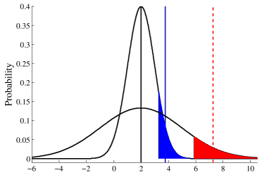
Figure 1: Comparison of two distributions with identical expectations and different $\text{CVaR}_{0.9}$ values. The filled-in regions illustrate the quantiles, while the vertical lines indicate the expectations and conditional values-at-risk.

The CVaR has been studied extensively [6, 37], and is known to have favorable mathematical properties such as coherence [47]. It has also been used in many practical applications, in finance and other domains [48].

The next lemma gives sample complexity results for the preceding four risk measures.

Lemma 3

Given $s\in\mathbb{{S}}$, $a\in\mathbb{A},$ $J\in B\left(\mathbb{S};J_{\max}\right)$, $\varepsilon>0$ and $m\geq 1$. Denote $d(\rho,\hat{\rho}_{m})=|\rho(J(Y^{s,a}))-\hat{\rho}_{m}(\{J(Y_{j}^{s,a})\}^{m}_{j=1})|$.

1. For mean-deviation or mean-semideviation, we have

   $$\mathbb{P}(d(\rho,\hat{\rho}_{m})>\varepsilon)\leq 2(e^{-x}+e^{-y}+e^{-z}),$$

   where $x=m\varepsilon^{2}/(\sqrt{2}J_{\max})^{2},$ $y=m\varepsilon^{2}/(\sqrt{2}bp(1+C)J_{\max}^{p})^{2}$ and $z=m\varepsilon^{2}/(\sqrt{2}bp(1+C)J_{\max}^{2p-1})^{2}$ with constant $C>0.$

2. For coherent optimized certainty equivalent, we have

   $$\mathbb{P}(d(\rho,\hat{\rho}_{m})>\varepsilon)\leq 2\left(1+\frac{4\beta_{2}}{\varepsilon}\right)\exp\left[\frac{-m\varepsilon^{2}}{(\sqrt{2}u(J_{\max}))^{2}}\right].$$

3. For conditional value-at-risk, we have

   $$\mathbb{P}(d(\rho,\hat{\rho}_{m})>\varepsilon)\leq 2\left(1+\frac{4}{\varepsilon(1-\alpha)}\right)\exp\left[\frac{-m(\varepsilon(1-\alpha))^{2}}{(\sqrt{2}(2-\alpha)J_{\max})^{2}}\right].$$

V Convergence analysis via stochastic dominance

In this section, we expand upon our convergence analysis to explore the tradeoff between sample complexity and convergence rate. In Section III we computed the required number of iterations to reach a desired accuracy given a certain error tolerance, and then computed the number of samples required to stay within this error tolerance in every iteration. We relax this idea in this section and instead we allow the approximation error in iterations to exceed this error tolerance. In [24], a stochastic dominance technique is developed to study this situation. The original work in [24] was specific to finite state and action space MDPs. Now extend this argument to show that this method is applicable to our present setting.

Theorems 1 and 2 give an estimate for the error $\|J^{\widehat{\pi}_{k}}-J^{*}\|_{p,\varrho}$ and $\|\widehat{J}_{K}-J^{*}\|_{\infty}$ based on fixing $\varepsilon>0$ and assuming $\|\varepsilon_{k}\|\leq\varepsilon$ for all iterations $k=0,\ldots,K-1$. The next sample complexity result allows for a smaller number of samples in each iteration, but requires a larger overall number of iterations.

Theorem 3

Let Assumption 1 and 2 hold. Given $\epsilon_{g}\in\left(0,1\right),$ $\delta\in\left(0,1\right)$ and let $\delta_{1}+2\delta_{2}\leq\delta.$ Choose $K$ such that

$$K\geq\log\left(\frac{1}{\delta_{2}\mu_{\min}}\right),$$

where $\mu_{\min}\triangleq\min_{\eta}\mu\left(\eta\right)$ with $\mu\left(\eta\right)$ given in Lemma 13.

1. Under Assumption 4 and 5, select $\varepsilon<\epsilon_{g},$ $\epsilon$ and $m$ such that

   $$\epsilon\leq\frac{\varepsilon}{2\left(\kappa_{c}+\gamma\kappa_{\mu}J_{\max}\right)}\quad\text{and}\quad\theta\left(\frac{\varepsilon}{2\gamma},m\right)\leq\frac{\delta_{1}}{\left|\mathbb{A}\right|\left|\mathcal{S}\right|}.$$

   Then we have $\mathbb{P}(\|\widehat{J}_{K}-J^{*}\|_{\infty}>\epsilon_{g})\leq\delta$.

2. Under Assumption 3, select $\varepsilon<\epsilon_{g}-d_{p,\mu}(T\mathcal{F},\mathcal{F}),$ $n$ and $m$ such that

   $$n>128\left(\frac{8J_{\max}}{\varepsilon}\right)^{2p}\left(\log\left(1/\delta_{1}\right)+\log\left(32\mathcal{N}_{0}\left(n\right)\right)\right)$$

   and

   $$\theta\left(\varepsilon/4,m\right)\leq\frac{\delta_{1}}{4n\left|\mathbb{A}\right|}$$

   where $\mathcal{N}_{0}(n)=\mathcal{N}(8^{-1}({\varepsilon}/{4})^{p},\mathcal{F},n,\mu).$ Then we have $\mathbb{P}(\|J^{\widehat{\pi}_{K}}-J^{*}\|_{p,\varrho}>\epsilon_{g})\leq\delta$.

Theorem 2 and Theorem 3 part 1) offer two different convergence analysis. We now confirm our claim that the stochastic dominance analysis requires a smaller number of samples in each iteration. First, we take $\theta\left(\varepsilon,m\right)=Ce^{-m\varepsilon^{2}}$ where $C>0$ is some constant, and compute the minimal number of samples $m_{1}$ required by Theorem 2 and samples $m_{2}$ required for the stochastic dominance analysis:

$$m_{1}=\frac{4\gamma^{2}}{\left[\varepsilon\left(1-\gamma\right)-2\gamma^{K}J_{\max}\left(1-\gamma\right)\right]^{2}}\log\frac{\left|\mathbb{A}\right|\left|\mathcal{S}\right|C}{1-\left(1-\delta\right)^{1/K}},$$

$$m_{2}=\frac{4\gamma^{2}}{\varepsilon^{2}}\log\frac{\left|\mathbb{A}\right|\left|\mathcal{S}\right|C}{\delta-2/e^{K}\mu_{\min}},$$

where $\mu_{\min}=\min\left\{\mu_{1},\mu_{2}\right\},$ with $\mu_{1}=(1-\delta)^{(\lceil J_{\max}/\varepsilon\rceil-1)/K}$ and $\mu_{2}=[1-(1-\delta)^{1/K}](1-\delta)^{(\lceil J_{\max}/\varepsilon\rceil-2)/K}$.

To verify our claim, we next allow $K$ to be arbitrarily large and show $m_{1}\geq m_{2}$ in the following. First, we need to show $e^{K}\mu_{\min}\rightarrow+\infty$ as $K\rightarrow+\infty.$ Note that for constant $d\in\left(0,1\right)$ and $K>0,$ we have

$$(1-d^{1/K})(1+d^{1/K}+d^{2/K}+\dots+d^{\left(K-1\right)/K})=1-d,$$

and thus $1-d^{1/K}\geq{(1-d)}/{K}.$ We then obtain that $e^{K}(1-d^{1/K})\geq{[e^{K}(1-d)]}/{K}\rightarrow+\infty$ as $K\rightarrow+\infty.$ Since $\mu_{\min}\in\left(0,1\right),$ we conclude that $e^{K}\mu_{\min}\rightarrow+\infty$ as $K\rightarrow+\infty.$ Finally, by letting $K$ be arbitrarily large, we have $m_{1}/m_{2}\approx{1}/{(1-\gamma)^{2}},$ which implies the stochastic dominance analysis requires a smaller number of samples in each iteration given sufficiently large amount of iterations $K.$

The sample comparison for analysis in Theorem 1 and Theorem 3 2) is nontrivial because it does not follow from a contraction argument. This discussion is left for future work.

VI Proofs of main results

This section is organized as follows. In Section VI-B and VI-A, we provide details for two types of analysis, i.e., $p-$norm and supremum analysis, followed by their alternative stochastic dominance convergence analysis in Section VI-C. Proofs of all technical results can be found in the Appendix.

VI-A Analysis in $p-$norm

The idea of analysis in $p-$norm is to show that (i) the approximation errors stay small with high probability in each iteration provided that $m,n$ are sufficiently large, and (ii) if the errors in each iteration are small then the final error will be small when $K$, the number of iterations, is big enough. To show (i), we provide a lemma which gives us a probabilistic guarantee on the approximation error introduced in a single iteration of our algorithm.

Lemma 4

Let Assumption 1 and 2 hold. Fix real number $p\in[1,+\infty),$ integers $n,m\geq 1,$ $\mu\in\mathcal{P}\left(\mathbb{S}\right)$ and $\mathcal{F}\subset B\left(\mathbb{S};J_{\max}\right).$ Pick any $J\in B\left(\mathbb{S};J_{\max}\right)$ and let $\widehat{J}_{k+1}=\widehat{J}_{k+1}\left(J,n,m,\mu,\mathcal{F}\right)$ be defined by Equation (8). Let $\mathcal{N}_{0}\left(n\right)=\mathcal{N}\left(8^{-1}\left({\varepsilon}/{4}\right)^{p},\mathcal{F},n,\mu\right).$ Then for any $\varepsilon,\delta>0,$

$$\|\widehat{J}_{k+1}-T\widehat{J}_{k}\|_{p,\mu}\leq d_{p,\mu}(T\widehat{J}_{k},\mathcal{F})+\varepsilon$$

holds w.p. at least $1-\delta$ provided that

$$n>128\left({8J_{\max}}/{\varepsilon}\right)^{2p}\left(\log\left(1/\delta\right)+\log\left(32\mathcal{N}_{0}\left(n\right)\right)\right)$$

and $m$ satisfying

$$\theta\left(\frac{\varepsilon}{4},m\right)\leq\frac{\delta}{4n\left|\mathbb{A}\right|}.$$

Lemma 4 shows that with high probability, $\widehat{J}_{k+1}$ is a good approximation to $T\widehat{J}_{k}$ provided that some element of $\mathcal{F}$ is close to $T\widehat{J}_{k}$ and if the number of samples is sufficiently large. In other words, the lemma states the finite-sample bound for a single iterate.

For risk measures defined in Section IV, we have the following error bound for each iteration.

Corollary 1

Let Assumptions 1 and 2 hold. Given a real number $p\in[1,+\infty),$ $\mu\in\mathcal{P}(\mathbb{S}),$ $\mathcal{F}\subset B(\mathbb{S};J_{\max}).$ Pick any $J\in B\left(\mathbb{S};J_{\max}\right)$ and let $\widehat{J}_{k+1}=\widehat{J}_{k+1}\left(J,n,m,\mu,\mathcal{F}\right)$ be defined by Equation (8). Let $\mathcal{N}_{0}(n)=\mathcal{N}(8^{-1}({\varepsilon}/{4})^{p},\mathcal{F},n,\mu).$ Then for any $\varepsilon,\delta>0,$

$$\|\widehat{J}_{k+1}-T\widehat{J}_{k}\|_{p,\mu}\leq d_{p,\mu}(T\widehat{J}_{k},\mathcal{F})+\varepsilon$$

holds w.p. at least $1-\delta$ provided that

$$n>128\left(\frac{8J_{\max}}{\varepsilon}\right)^{2p}\left(\log\left(1/\delta\right)+\log\left(32\mathcal{N}_{0}\left(n\right)\right)\right)$$

and $m$ satisfying

1. $$m>\frac{32m^{\prime}}{\varepsilon^{2}}\left(\log\left(1/\delta\right)+\log\left(8n\left|\mathbb{A}\right|\right)\right),$$

   where $m^{\prime}=\min\{((1+C)J_{\max}^{p})^{2},(bp(1+C)J_{\max}^{2p-1})^{2},J_{\max}^{2}\}$ with constant $C>0$ for mean-deviation or mean-semideviation risk function $\rho.$

2. $$m>32(u(J_{\max})/\varepsilon)^{2}(\log\left(1/\delta\right)+\log\left(8n\left|\mathbb{A}\right|\right)+\log(1+16\beta_{2}/\varepsilon))$$

   for coherent optimized certainty equivalent $\rho.$

3. $$m>32\left(\frac{\left(2-\alpha\right)J_{\max}}{\left(1-\alpha\right)\varepsilon}\right)^{2}(\log\left(1/\delta\right)+\log\left(8n\left|\mathbb{A}\right|\right)+\log\left(1+16/{\varepsilon\left(1-\alpha\right)}\right))$$

   given CVaR with parameter $\alpha\in[0,1).$

The proof below puts (i) and (ii) together and gives the main result.

Proof:

The proof essentially follows the proof of [22, Theorem 2] and states PAC-bounds on the sample size of sampling-based approximate value iteration. First, we state the key piece of the derivation of the error bounds. Recall that a stochastic kernel is $Q\mbox{ : }B\left(\mathbb{S};J_{\max}\right)\rightarrow B\left(\mathbb{S};J_{\max}\right)$ such that $[QJ](s)$ is an expectation of $J\left(Y\right)$ w.r.t. some probability distribution, for all states $s\in\mathbb{S}$.

Lemma 5

1. For any $\widehat{J}_{k}\in B\left(\mathbb{S};J_{\max}\right)$, there is a stochastic kernel $Q^{\pi_{k}}$ such that $T^{\pi^{*}}\widehat{J}_{k}-T^{\pi^{*}}J^{*}\leq\gamma Q^{\pi_{k}}(\widehat{J}_{k}-J^{*})$.

2. For any $\widehat{J}_{k}\in B\left(\mathbb{S};J_{\max}\right)$, there is a stochastic kernel $Q^{\pi_{k}^{*}}$ such that $T^{\hat{\pi}_{k}}\widehat{J}_{k}-T^{\hat{\pi}_{k}}J^{*}\geq\gamma Q^{\pi_{k}^{*}}(\widehat{J}_{k}-J^{*})$.

Next, we apply Lemma 5 and adapt [22, Lemma 3] to obtain point-wise error bounds (i.e., bounds hold for any state $s\in\mathbb{S}$) for $\{\widehat{J}_{k}\}_{k\geq 0}$ relative to $J^{*}$ with the approximation errors $\varepsilon_{k}$ defined in (6).

Lemma 6

Choose $K\geq 1$. We have

$$J^{\widehat{\pi}_{K}}-J^{*}\leq 2Q_{0}\left\{\sum_{k=0}^{K-1}\gamma^{K-k}Q_{1}|\varepsilon_{k}|+\gamma^{K+1}Q_{2}|\widehat{J}_{0}-J^{*}|\right\}$$

where

$$Q_{0}= (I-\gamma Q^{\hat{\pi}_{K}})^{-1},$$

$$Q_{1}= (Q^{\pi_{K}}Q^{\pi_{K-1}}\dots Q^{\pi_{k+1}}+Q^{\hat{\pi}_{K}}Q^{\pi_{K-1}^{*}}Q^{\pi_{K-2}^{*}}\dots Q^{\pi_{k+1}^{*}})/2,$$

$$Q_{2}= (Q^{\pi_{K}}Q^{\pi_{K-1}}\dots Q^{\pi_{0}}+Q^{\hat{\pi}_{K}}Q^{\pi_{K-1}^{*}}Q^{\pi_{K-2}^{*}}\dots Q^{\pi_{0}^{*}})/2.$$

We need to adapt [22, Lemma 3] to get the previous lemma because the Bellman operator $T$ is not a contraction operator w.r.t. the $\mathcal{L}_{p}$ norm for $1\leq p<\infty$. The preceding point-wise error bounds suggest that if the sequence of errors $\{\varepsilon_{k}\}_{k\geq 0}$ is small then $\widehat{J}_{K}$ should be close to $J^{*}$ and the greedy policy $\widehat{\pi}_{K}$ w.r.t. $\widehat{J}_{K}$ should be close to optimal. The next lemma gives $\mathcal{L}_{p}$ bounds by using the point-wise error bounds in Lemma 6.

Lemma 7

Let Assumption 3 hold. For any $\eta>0$, there exists $K$ that is linear in $\log\left(1/\eta\right)$ and $\log J_{\max}$ such that, if the $\mathcal{L}_{p}\left(\mu\right)-$norm of the approximation errors is bounded by some $\varepsilon$ ($\|\varepsilon_{k}\|_{p,\mu}\leq\varepsilon$ for all $0\leq k<K$) then

$$\left\|J^{\widehat{\pi}_{K}}-J^{*}\right\|_{p,\varrho}\leq\frac{2\gamma}{\left(1-\gamma\right)^{2}}C_{\varrho,\mu}^{1/p}\varepsilon+\eta.$$

Next, we state a technical lemma without its proof.

Lemma 8 ([22, Lemma 5])

Assume that $X,Y$ are independent random variables taking values in the respective measurable spaces, $\mathcal{X}$ and $\mathcal{Y}$. Let $g:\mathcal{X}\times\mathcal{Y}\rightarrow\mathbb{R}$ be a Borel-measurable function such that $\mathbb{E}[g\left(X,Y\right)]$ exists. Assume that for all $y\in\mathcal{Y},$ $\mathbb{E}[g\left(X,y\right)]\geq 0$. Then $\mathbb{E}[g(X,Y)|Y]\geq 0$ holds, too, w.p. $1.$

Fix $\varepsilon,\delta>0.$ The aim is to show that by selecting the number of iterates $K$, and the number of samples $m,n$ large enough, the bound

$$\left\|J^{\widehat{\pi}_{K}}-J^{*}\right\|_{p,\varrho}\leq\frac{2\gamma}{\left(1-\gamma\right)^{2}}C_{\varrho,\mu}^{1/p}d_{p,\mu}\left(T\mathcal{F},\>\mathcal{F}\right)+\varepsilon$$ (10)

holds w.p. at least $1-\delta.$ Note that by construction the iterates $\widehat{J}_{k}$ remain bounded by $J_{\max}.$ By Lemma 7, under Assumption 3, for all those events, where the error $\varepsilon_{k}=T\widehat{J}_{k}-\widehat{J}_{k+1}$ of the $k^{th}$ iterate is below (in $\mathcal{L}_{p}\left(\mu\right)-$norm) some level $\varepsilon_{0},$ we have

$$\left\|J^{\widehat{\pi}_{K}}-J^{*}\right\|_{p,\varrho}\leq\frac{2\gamma}{\left(1-\gamma\right)^{2}}C_{\varrho,\mu}^{1/p}\varepsilon_{0}+\eta,$$ (11)

provided that $K=\Omega\left(\log\left(1/\eta\right)\right).$ Now choose

$$\varepsilon^{\prime}=\frac{\varepsilon\left(1-\gamma\right)^{2}}{4\gamma C_{\varrho,\mu}^{1/p}}\quad\mbox{and }\quad\eta=\frac{\varepsilon}{2}.$$

Let $f\left(\varepsilon,\delta\right)$ denote the function that gives lower bounds on $m,n$ in Lemma 4 based on the value of the desired estimation error $\varepsilon$ and confidence $\delta.$ Let $\left(n,m\right)\geq f\left(\varepsilon^{\prime},\delta/K\right).$ Let us denote the collection of random variables used in $k^{th}$ step by $s_{k}.$ Hence, $s_{k}$ consists of the $n$ sampled states, as well as $\left|\mathbb{A}\right|\times n\times m$ next states. Further, introduce the notation $\widehat{J}\left(J,s_{k}\right)$ to denote the result of solving the optimization problems (7) and (8) based on the samples $s_{k}$ and starting from the risk-to-go $J\in B\left(\mathbb{S};J_{\max}\right).$ By Lemma 4,

$$\mathbb{P}(\|\widehat{J}(J,s_{k})-TJ\|_{p,\mu}\leq d_{p,\mu}(TJ,\mathcal{F})+\varepsilon^{\prime})\geq 1-\delta/K.$$

Apply Lemma 8 with $X=s_{k},$ $Y=\widehat{J}_{k}$ and $g\left(s,J\right)=\mathbb{I}_{\left\{\|\widehat{J}\left(J,s\right)-TJ\|_{p,\mu}\leq d_{p,\mu}\left(TJ,\mathcal{F}\right)+\varepsilon^{\prime}\right\}}-\left(1-\delta/K\right).$ Since $s_{k}$ is independent of $\widehat{J}_{k},$ the lemma can be applied. Therefore,

$$\mathbb{P}(\|\widehat{J}(\widehat{J}_{k},s_{k})-T\widehat{J}_{k}\|_{p,\mu}\leq d_{p,\mu}(T\widehat{J}_{k},\mathcal{F})+\varepsilon^{\prime}\big{|}\widehat{J}_{K})\geq 1-\delta/K.$$

Taking expectation of both sides gives

$$\mathbb{P}(\|\widehat{J}(\widehat{J}_{k},s_{k})-T\widehat{J}_{k}\|_{p,\mu}\leq d_{p,\mu}(T\widehat{J}_{k},\mathcal{F})+\varepsilon^{\prime})\geq 1-\delta/K.$$

Since $\widehat{J}(\widehat{J}_{k},s_{k})=\widehat{J}_{k+1}$ and $\varepsilon_{k}=T\widehat{J}_{k}-\widehat{J}_{k+1},$ we thus have

$$\left\|\varepsilon_{k}\right\|_{p,\mu}\leq d_{p,\mu}\left(TJ,\mathcal{F}\right)+\varepsilon^{\prime}$$

holds except for a set of bad events $B_{k}$ of measure at most $\delta/K.$ Hence, above inequality holds simultaneously for $k=1,\dots,K$ except for the events in $B=\cup_{k}B_{k}.$ Note that

$$\mathbb{P}\left(B\right)\leq\sum_{k=1}^{K}\mathbb{P}\left(B_{k}\right)\leq\delta.$$

Now pick any event in the complement of $B.$ Thus, for such an event (11) holds when $\varepsilon_{0}=d_{p,\mu}\left(TJ,\mathcal{F}\right)+\varepsilon^{\prime}.$ Plugging in the definition of $\varepsilon^{\prime}$ and $\eta$ we obtain (10). ∎

VI-B Analysis in supremum norm

The convergence analysis in the supremum norm follows from the fact that $T$ is a contracting operator as shown below.

Lemma 9

$|[TJ_{1}]\left(s\right)-[TJ_{2}]\left(s\right)|\leq\gamma\|J_{1}-J_{2}\|_{\infty}$ for all $s\in\mathbb{S}$ and $J_{1},$ $J_{2}\in B\left(\mathbb{S};J_{\max}\right)$.

It follows that $\|TJ-J^{*}\|_{\infty}\leq\gamma\|J-J^{*}\|_{\infty}$ for all $J\in B\left(\mathbb{S};J_{\max}\right)$. Next, given the true risk value $\rho(J(Y^{s,a}))$, we define $\overline{T}\mbox{ : }B\left(\mathbb{S};J_{\max}\right)\rightarrow\mathcal{F}$ as the Bellman operator corresponding to the finite state space MDP

$$\left[\overline{T}J\right]\left(s\right)=\min_{a\in\mathbb{A}}\left\{c(s,a)+\gamma\rho\left(J\left(Y^{s,a}\right)\right)\right\},\forall s\in\mathcal{S}.$$

The operator $\widetilde{T}\mbox{ : }B\left(\mathbb{S};J_{\max}\right)\rightarrow B\left(\mathbb{S};J_{\max}\right)$ is defined as an extension of $\overline{T}:$ for $s\in\mathbb{S},$ we can find $s^{\prime}\in\mathcal{S}$ and $\|s-s^{\prime}\|_{\infty}\leq\epsilon,$ such that

$$[\widetilde{T}J](s)=[\overline{T}J](s^{\prime})$$

by Assumption 5. Moreover, we use a random operator $\widehat{T}:B\left(\mathbb{S};J_{\max}\right)\rightarrow B\left(\mathbb{S};J_{\max}\right)$ to represent steps 1, 2, and 3 of Algorithm 1, i.e., the state space sampling over an $\epsilon-$net $\mathcal{S}$, risk-to-go estimation $\{\widetilde{J}_{k+1}\left(s\right)\}_{s\in\mathcal{S}}$ from $\hat{J}_{k}$, and function extension to produce $\widehat{J}_{k+1}\in B\left(\mathbb{S};J_{\max}\right)$ (we leave the dependence on the sample size $m\geq 1$ in $\widehat{T}$ implicit for cleaner notation). The iterates $\{\widehat{J}_{k}\}_{k\geq 0}$ of our approximate value iteration algorithm then satisfy $\widehat{J}_{k+1}=\widehat{T}\widehat{J}_{k}$ for all $k\geq 0$.

Under Assumption 1, the risk-to-go functions are uniformly bounded by $J_{\max},$ and thus the worst error satisfies $\|\widehat{J}_{K}-J^{*}\|_{\infty}\leq J_{\max}.$ When we use the random operator $\widehat{T}$, the error $\|\widehat{T}J-TJ\|_{\infty}$ is incurred and we have

$$\|\widehat{T}J-J^{*}\|_{\infty} \leq\|TJ-J^{*}\|_{\infty}+\|\widehat{T}J-TJ\|_{\infty}$$ (12)

$$\leq\gamma\|J-J^{*}\|_{\infty}+\|\widehat{T}J-TJ\|_{\infty}.$$

If the stochastic error term $\|\widehat{T}J-TJ\|_{\infty}$ is small then $\widehat{T}$ is nearly a contraction operator. Based on this observation, inequality (12) yields our $\infty-$norm convergence analysis. The following lemma bounds $\|\widehat{T}J-TJ\|_{\infty}.$ Its proof relies on the fact $\|\widehat{T}J-TJ\|_{\infty}\leq\|\widehat{T}J-\widetilde{T}J\|_{\infty}+\|\widetilde{T}J-TJ\|_{\infty}.$

Lemma 10

Let $\varepsilon>0.$ Under Assumption 1, 2, 4 and 5, if the $\epsilon-$net is chosen such that $\epsilon\leq{\varepsilon}/{\left(2\kappa_{c}+2\gamma\kappa_{\mu}J_{\max}\right)},$ we have

$$\mathbb{P}(\|\widehat{T}J-TJ\|_{\infty}\leq\varepsilon)\geq 1-n|\mathbb{A}|\theta({\varepsilon}/({2\gamma}),m).$$

The convergence result for the supremum norm algorithm then follows immediately, as shown below.

Proof:

Let the approximation errors $\varepsilon_{k}$ defined in (6) satisfy $\left\|\varepsilon_{k}\right\|_{\infty}\leq\varepsilon$ for all $k=0,\dots,K-1,$ and denote $p_{m,n}\left(\varepsilon\right)=n\left|\mathbb{A}\right|\theta\left({\varepsilon}/(2\gamma),m\right).$ Starting with $K=1$, we have

$$\|\widehat{J}_{1}-J^{*}\|_{\infty} =\|\widehat{T}\widehat{J}_{0}-J^{*}\|_{\infty}$$

$$\leq\|T\widehat{J}_{0}-J^{*}\|_{\infty}+\|\widehat{T}\widehat{J}_{0}-T\widehat{J}_{0}\|_{\infty}$$

$$\leq\gamma\|\widehat{J}_{0}-J^{*}\|_{\infty}+\varepsilon,$$

with probability at least $1-p_{m,n}\left(\varepsilon\right)$ by Lemma 9 and 10. For $K=2$, by the union bound of probability, we have

$$\|\widehat{J}_{2}-J^{*}\|_{\infty} \leq\gamma\|\widehat{J}_{1}-J^{*}\|_{\infty}+\varepsilon$$

$$\leq\gamma^{2}\|\widehat{J}_{0}-J^{*}\|_{\infty}+\gamma\varepsilon+\varepsilon,$$

with probability at least $1-2p_{m,n}\left(\varepsilon\right)$. By induction, for $K\geq 1$,

$$\|\widehat{J}_{K}-J^{*}\|_{\infty} \leq\gamma\|\widehat{J}_{K-1}-J^{*}\|_{\infty}+\varepsilon$$

$$\leq\gamma^{K}\|\widehat{J}_{0}-J^{*}\|_{\infty}+\sum_{k=0}^{K-1}\gamma^{K-k-1}\varepsilon$$

with probability at least $1-Kp_{m,n}\left(\varepsilon\right)$.

Note that $\sum_{k=0}^{K-1}\gamma^{K-k-1}\leq 1/\left(1-\gamma\right)$ for all $K\geq 1$ and $\|\widehat{J}_{0}-J^{*}\|_{\infty}\leq J_{\max}.$ We obtain

$$\mathbb{P}\left(\|\widehat{J}_{K}-J^{*}\|_{\infty}\leq\gamma^{K}J_{\max}+{\varepsilon}/{(1-\gamma)}\right)\geq 1-Kp_{m,n}\left(\varepsilon\right).$$

∎

VI-C Analysis via stochastic dominance

We first recall the approximation error $\varepsilon_{k}$ defined in Equation (6) that appears in approximate value iteration:

$$\widehat{J}_{k+1}=T\widehat{J}_{k}-\varepsilon_{k},\quad\forall k\geq 0.$$

The following inequalities form the foundation of our stochastic dominance analysis, they give bounds on the approximation error for both the supremum and $p-$norms.

Lemma 11

1. Let Assumption 1 hold. If $\left\|\varepsilon_{k}\right\|_{\infty}\leq\varepsilon$ for all $0\leq k<K,$ we have

   $$\|\widehat{J}_{K}-J^{*}\|_{\infty}\leq\gamma^{K}J_{\max}+\frac{\varepsilon}{1-\gamma}.$$ (13)

2. Let Assumption 1 and 3 hold. If $\left\|\varepsilon_{k}\right\|_{p,\mu}\leq\varepsilon$ for all $0\leq k<K,$ we have

   $$\|J^{\widehat{\pi}_{K}}-J^{*}\|_{p,\varrho}\leq \frac{2\gamma}{\left(1-\gamma\right)^{2}}[C_{\varrho,\mu}^{1/p}\varepsilon+\gamma^{K/p}(1-\gamma)^{1/p}(1-\gamma^{K+1})^{1-1/p}J_{\max}].$$ (14)

We remark that the above results hold by assuming that the approximation error in all iterations $k=0,\dots,K-1$ falls below the tolerance $\varepsilon.$ The iteration count $K$ is chosen to control the error $J_{\max}.$

Note that the RHS of the inequalities (13) and (14) do not depend on the initial error between $\widehat{J}_{0}$ and $J^{*}$, it depends on the worst-case error $J_{\max}$. For the rest of this section, let us fix an error tolerance $\varepsilon>0$. Once $\varepsilon>0$ is fixed, we consider an iteration “good” if the error falls below $\varepsilon$, and we consider an iteration to be “bad” if the error exceeds $\varepsilon$. Once $\varepsilon>0$ is fixed, inequalities (13) and (14) give us guidance on how many “good” iterations $K$ are required to reach a desired approximation error. Again, this number $K$ can be chosen directly from the inequalities (13) and (14), even though the latter inequality does not follow from a contraction argument as it is originally done in $\infty-$norm in [24].

Now we are in a position to use our stochastic dominance convergence analysis. Consider a probability space $(\Omega,\mathcal{B}(\Omega),P)$ where $\Omega$ is a sample space with elements denoted $\omega\in\Omega$, $\mathcal{B}\left(\Omega\right)$ is the Borel $\sigma-$algebra on $\Omega$, and $P$ is a probability distribution on $\left(\Omega,\mathcal{B}(\Omega)\right)$. In our upcoming algorithms, $\left(\Omega,\mathcal{B}(\Omega),P\right)$ corresponds to the randomness used to drive one round of simulation. We are interested in repeated samples from $\left(\Omega,\mathcal{B}(\Omega),P\right)$, so we define the space of sequences $(\Omega^{\infty},\mathcal{B}(\Omega^{\infty}),\mathcal{P})$ where $\Omega^{\infty}=\times_{k=0}^{\infty}\Omega$ with elements denoted $\boldsymbol{\omega}=(\omega_{k})_{k\geq 0}$, $\mathcal{B}(\Omega^{\infty})=\times_{k=0}^{\infty}\mathcal{B}(\Omega)$, and $\mathcal{P}$ is the probability measure on $(\Omega^{\infty},\mathcal{B}(\Omega^{\infty}))$ guaranteed by the Kolmogorov extension theorem applied to $P$. Let $\{X_{k}\}_{k\geq 0}$ be a stochastic process on $(\Omega^{\infty},\mathcal{B}(\Omega^{\infty}),\mathcal{P})$ with the integer-valued state space $\{0,1,\ldots,K^{*}\}$ where $K^{*}$ is an upper bound on $\{X_{k}\}_{k\geq 0}$.

Let $\left\lceil x\right\rceil$ denote the smallest integer greater than or equal to $x\in\mathbb{R}$ and $\epsilon_{g}>0$ be a granularity. The stochastic process $\{X_{k}\}_{k\geq 0}$ on a discrete and finite state space is defined by

$$X_{k}=\left\lceil\|J^{k}-J^{*}\|/\epsilon_{g}\right\rceil,$$

where $J^{k}=\widehat{J}_{k}$ when $\|\cdot\|$ is the $\infty-$norm and $J^{k}=J^{\widehat{\pi}_{k}}$ when $\|\cdot\|$ is the $p-$norm. Since $\|J^{k}-J^{*}\|\leq J_{\max},$ we define a constant

$$K^{*}\triangleq\left\lceil{J_{\max}}/{\epsilon_{g}}\right\rceil.$$

Notice that $K^{*}$ is the smallest number of intervals of length $\epsilon_{g}$ needed to cover the interval $[0,J_{\max}].$ By construction, the stochastic process $\{X_{k}\}_{k\geq 0}$ is restricted to the finite state space $\{\eta\in\mathbb{N}:0\leq\eta\leq K^{*}\}.$ If we could understand the behavior of the stochastic process $\{X_{k}\}_{k\geq 0},$ then we could analysis the convergence of $\{\|J^{k}-J^{*}\|\}_{k\geq 0}.$ Throughout this paper, $\{X_{k}\}_{k\geq 0}$ will represent the error between a risk-to-go function estimate and the optimal risk-to-go function in the simulation-based approximate value iteration algorithms.

Consider the state space $\{1,2,\ldots,K^{*}\},$ where state $K^{*}$ corresponds to the worst case starting error $J_{\max}$ and state $1$ corresponds to the desired approximation error. In other words, if we have a string of $K^{*}$ “good” iterations, we are able to reach our desired performance. We are thus interested in studying the convergence of $\{X_{k}\}_{k\geq 0}$ to zero. We next make an assumption about the behavior of $\{X_{k}\}_{k\geq 0}$.

Assumption 6

For $\varepsilon>0$ and all $k\geq 0$, $\mathbb{P}(\|J^{k}-J^{*}\|\leq\varepsilon)\geq p$ with probability $p\in(0,1)$. Here $J^{k}=\widehat{J}_{k}$ when $\|\cdot\|$ is the $\infty-$norm and $J^{k}=J^{\widehat{\pi}_{k}}$ when $\|\cdot\|$ is the $p-$norm.

The choice of $p$ in Assumption 6 depends on the specifics of $\left\{X_{k}\right\}_{k\geq 0}$, and we now discuss: in the supremum-norm analysis, we choose $p\triangleq 1-n|\mathbb{A}|\theta({\varepsilon}/{(2\gamma)},m)$ since

$$\mathbb{P}(\|\widehat{T}\widehat{J}_{k}-T\widehat{J}_{k}\|_{\infty}\leq\varepsilon)\geq 1-n\left|\mathbb{A}\right|\theta({\varepsilon}/{(2\gamma)},m)$$

from Lemma 10; in the $p-$norm analysis, we set $p\triangleq 1-\delta$ since

$$\mathbb{P}(\|\widehat{J}_{k+1}-T\widehat{J}_{k}\|_{p,\mu}\leq d_{p,\mu}(T\widehat{J}_{k},\mathcal{F})+\varepsilon)\geq 1-\delta$$

from Lemma 4. As shown before, we are able to control $p$ in Assumption 6 by improving the quality of our simulation-based approximate value iteration algorithms with more samples and also by choosing a richer functional family.

Based on Assumption 6, we can construct a “dominating” Markov chain $\left\{Y_{k}\right\}_{k\geq 0}$ to help us analyze the behavior of $\left\{X_{k}\right\}_{k\geq 0}$. We construct $\left\{Y_{k}\right\}_{k\geq 0}$ on $\left(\mathbb{N}^{\infty},\mathcal{N}\right)$, the canonical measurable space of trajectories on $\mathbb{N}$, so $Y_{k}\mbox{ : }\mathbb{N}^{\infty}\rightarrow\mathbb{N}$. We will use $\mathcal{Q}$ to denote the probability measure of $\{Y_{k}\}_{k\geq 0}$ on $\left(\mathbb{N}^{\infty},\mathcal{N}\right)$. Since $\left\{Y_{k}\right\}_{k\geq 0}$ will be a Markov chain by construction, the probability measure $\mathcal{Q}$ is completely determined by an initial distribution on $\mathbb{N}$ and a transition kernel for $\left\{Y_{k}\right\}_{k\geq 0}$ denoted $\mathfrak{Q}$. We restrict $\left\{Y_{k}\right\}_{k\geq 0}$ to the finite state space $\left\{1,2,\ldots,K^{*}-1,K^{*}\right\}$. We then define:

$$Y_{k+1}=\begin{cases}\max\left\{Y_{k}-1,1\right\},&\mbox{w.p. }p,\\ K^{*},&\mbox{w.p. }1-p,\end{cases}$$

where $p$ is the same one from Assumption 6 and is the probability of a “good” iteration (where the error falls bellow $\epsilon_{g}$). In words, $\left\{Y_{k}\right\}_{k\geq 0}$ moves one unit closer to state 1 with probability $p$ (corresponding to a “good” iteration) or moves back to the starting worst-case error $J_{\max}$ with probability $1-p$, corresponding to a “bad” iteration. Notice that this bound is extremely conservative, because we always assume that a “bad” iteration is so bad that it resets the entire process. Moreover, any time we are in state $1$, we know that we have reached the desired performance level: if we are in state $1$, and we have a “good” iteration, then we remain in state $1$ (since the RHS of both inequalities (13) and (14) is decreasing in $K$, so more “good” iterations than we need does not increase the approximation error).

We now show that $\{X_{k}\}_{k\geq 0}$ and $\{Y_{k}\}_{k\geq 0}$ have a stochastic dominance relationship. The following definition gives the notion of (first-order) stochastic dominance (see [49]).

Definition 1

Let $X$ and $Y$ be two real-valued random variables. Y stochastically dominates $X,$ written as $X\leq_{st}Y,$ when $\mathbb{P}\left(X\geq\theta\right)\leq\mathbb{P}\left(Y\geq\theta\right)$ for all $\theta$ in the support of $Y.$

The theorem below compares the marginal distributions of $\{X_{k}\}_{k\geq 0}$ and $\{Y_{k}\}_{k\geq 0}$ at all times $k\geq 0$ when the two stochastic processes $\{X_{k}\}_{k\geq 0}$ and $\{Y_{k}\}_{k\geq 0}$ start from the same state.

Lemma 12

Under Assumption 6. If $X_{0}=Y_{0},$ then $X_{k}\leq_{st}Y_{k}$ for all $k\geq 0.$

Next we compute the steady state distribution of the Markov chain $\{Y_{k}\}_{k\geq 0}.$ Let $\mu$ denote the steady state distribution of $Y=_{d}\lim_{k\rightarrow\infty}Y_{k},$ whose existence is guaranteed since $\{Y_{k}\}_{k\geq 0}$ is an irreducible Markov chain on a finite state space. Denote $\mu\left(i\right)=\mathcal{Q}\left(Y=i\right)$ for $i\in\left\{1,2,\ldots,K^{*}\right\}.$ The next lemma gives $\{\mu(i)\}_{i=1}^{K^{*}}.$

Lemma 13

Under Assumption 6. The values of $\{\mu\left(i\right)\}_{i=1}^{K^{*}}$ are $\mu\left(1\right)=p^{K^{*}-1},\quad\mu\left(K^{*}\right)=1-p,$ and $\mu\left(i\right)=\left(1-p\right)p^{K^{*}-i},$ $i=2,\dots,K^{*}-1.$

We are now ready to prove Theorem 3.

Proof:

First, we use Lemma 12 and 13 to derive an asymptotic result.

Proposition 1

For any $\delta_{1}\in\left(0,1\right).$

1. Select $\varepsilon<\epsilon_{g},$ $\epsilon$ and $m$ such that

   $$\epsilon\leq\frac{\varepsilon}{2\left(\kappa_{c}+\gamma\kappa_{\mu}J_{\max}\right)}$$

   and

   $$\theta\left(\frac{\epsilon_{g}}{2\gamma},m\right)\leq\frac{\delta_{1}}{\left|\mathbb{A}\right|\left|\mathcal{S}\right|},$$

   then $\limsup_{k\rightarrow\infty}\mathbb{P}(\|\widehat{J}_{k}-J^{*}\|_{\infty}>\epsilon_{g})\leq\delta_{1}.$

2. Select $\varepsilon<\epsilon_{g}-d_{p,\mu}\left(T\mathcal{F},\mathcal{F}\right),$ $n$ and $m$ such that

   $$n>128\left(\frac{8J_{\max}}{\varepsilon}\right)^{2p}\left(\log\left(1/\delta_{1}\right)+\log\left(32\mathcal{N}_{0}\left(n\right)\right)\right)$$

   and

   $$\theta\left(\varepsilon/4,m\right)\leq\frac{\delta_{1}}{4n\left|\mathbb{A}\right|},$$

   then $\limsup_{k\rightarrow\infty}\mathbb{P}(\|J^{\widehat{\pi}_{k}}-J^{*}\|_{p,\varrho}\geq\epsilon_{g})\leq\delta_{1}.$

Our earlier Lemma 13 gives the stationary distribution of $\{Y_{k}\}_{k\geq 0}$. To continue, we will use a mixing time argument to find out how “close” $\{Y_{k}\}_{k\geq 0}$ is to its stationary distribution as a function of time. The total variation distance between two probability measures $\mu$ and $\nu$ on $\mathbb{S}$ as

$$\bigl{\|}\mu-\nu\bigr{\|}_{TV}=\max_{S\subset\mathbb{S}}\bigl{|}\mu\left(S\right)-\nu\left(S\right)\bigr{|}=\frac{1}{2}\int_{\mathbb{S}}\bigl{|}\mu\left(ds\right)-\nu\left(ds\right)\bigr{|}.$$

Let $\mathcal{Q}_{k}$ be the marginal distribution of $Y_{k}$ on $\mathbb{N}$ at stage $k$ and $d\left(k\right)=\|\mathcal{Q}_{k}-\mu\|_{TV}$ be the total variation distance between $\mathcal{Q}_{k}$ and the steady state distribution $\mu.$ For $\delta_{2}>0,$ we define

$$t_{mix}\left(\delta_{2}\right)=\min\left\{k:d\left(k\right)\leq\delta_{2}\right\}$$

to be the minimum length of time needed for the marginal distribution of $Y_{k}$ to be within $\delta_{2}$ of the steady state distribution in total variation norm. By [50, Theorem 12.3], $t_{mix}\left(\delta_{2}\right)$ can be bounded as below.

Lemma 14

For any $\delta_{2}>0,$ we have

$$t_{mix}\left(\delta_{2}\right)\leq\log\left(\frac{1}{\delta_{2}\mu_{\min}}\right)$$

where $\mu_{\min}\triangleq\min_{\eta}\mu\left(\eta\right).$

Next, we use the above bound on mixing time to get a non-asymptotic bound.

Proposition 2

For $k\geq\log\left({1}{(\delta_{2}\mu_{\min})}\right),$ we have

1. $\mathbb{P}(\|\widehat{J}_{k}-J^{*}\|_{\infty}>\epsilon_{g})\leq 1+2\delta_{2}-\mu\left(1\right).$

2. $\mathbb{P}(\|J^{\widehat{\pi}_{k}}-J^{*}\|_{p,\varrho}>\epsilon_{g})\leq 1+2\delta_{2}-\mu\left(1\right).$

Finally, combing Proposition 1 and 2, we prove Theorem 3 1) and 2).

1. Let $\delta_{1},\delta_{2}>0$ and $\delta_{1}+2\delta_{2}\leq\delta.$ By the choice of $\varepsilon,\epsilon$ and $n$ in Proposition 1 1), we have

   $$\limsup_{k\rightarrow\infty}\mathbb{P}(\|\widehat{J}_{k}-J^{*}\|_{\infty}\geq\epsilon_{g})\leq 1-\mu(1)\leq\delta_{1}.$$

   For $k\geq\log({1}/{(\delta_{2}\mu_{\min})}),$ by Proposition 2 1), we have

   $$\mathbb{P}(\|\widehat{J}_{k}-J^{*}\|_{\infty}>\epsilon_{g})\leq 1+2\delta_{2}-\mu\left(1\right)\leq\delta_{1}+2\delta_{2}.$$

   Combining both inequalities, we obtain $\mathbb{P}(\|\widehat{J}_{k}-J^{*}\|_{\infty}>\epsilon_{g})\leq\delta$.

2. Let $\delta_{1},\delta_{2}>0$ and $\delta_{1}+2\delta_{2}\leq\delta.$ By the choice of $\varepsilon,m$ and $n$ in Proposition 1 2), we have

   $$\limsup_{k\rightarrow\infty}\mathbb{P}(\|J^{\widehat{\pi}_{k}}-J^{*}\|_{p,\varrho}\geq\epsilon_{g})\leq 1-\mu\left(1\right)\leq\delta_{1}.$$

   For $k\geq\log\left({1}{(\delta_{2}\mu_{\min})}\right),$ by Proposition 2 2), we have

   $$\mathbb{P}(\|J^{\widehat{\pi}_{k}}-J^{*}\|_{p,\varrho}>\epsilon_{g})\leq 1+2\delta_{2}-\mu\left(1\right)\leq\delta_{1}+2\delta_{2}.$$

   Combining both inequalities, we obtain $\mathbb{P}\left(\|J^{\widehat{\pi}_{k}}-J^{*}\|_{p,\varrho}>\epsilon_{g}\right)\leq\delta$.

∎

VII Numerical experiments

In this section, we report some simulation results that illustrate the performance of the methods developed in this paper.

VII-A An optimal maintaining problem

We consider a continuous one-dimensional optimal maintaining problem which is similar in spirit to the one in [22]. The state variable $s_{t}\in\mathbb{R}_{+}$ measures the accumulated utilization of a piece of equipment. The larger the value of the state, the worse the condition of the product; $s_{t}=0$ represents a brand new equipment. In addition, there is an absorbing “bad” state $s^{\text{bad}}$ that corresponds to broken equipment.

At each time $t\geq 0$, one can either keep ($a_{t}=\text{K}$) or repair ($a_{t}=\text{R}$) the existing equipment. The bad state models the situation where the equipment is broken and cannot be operated or repaired, and so $P(s_{t+1}^{\text{bad}}|s_{t}^{\text{bad}},a)=1$. When action K is chosen at time step $t$, the transition to a new state has a mixture distribution: with probability $q$ the new state is $s_{t+1}^{\text{bad}},$ and with probability $1-q$ next state follows the exponential density:

$$P\left(s_{t+1}|s_{t},\text{K}\right)=\begin{cases}\beta e^{-\beta\left(s_{t+1}-s_{t}\right)},\quad&\text{if}\,\,\mbox{$s_{t+1}\geq s_{t}$;}\\ 0,\quad&\text{otherwise.}\end{cases}$$

When action R is taken at time step $t\geq 0$, the next state follows

$$P\left(s_{t+1}|s_{t},\text{R}\right)=\begin{cases}\beta e^{-\beta s_{t+1}},\quad&\text{if}\,\,\mbox{$s_{t+1}\geq 0$;}\\ 0,\quad&\text{otherwise.}\end{cases}$$

The cost function is $c(s,\text{K})=f(s)$ where the monotonically increasing function $f\left(s\right)$ is the cost of operating the equipment when its condition is $s$. The cost associated with the repair of the equipment is independent of the state and is given by $c(s,\text{R})=C_{1}+f(0).$ Finally, the penalty of breaking the equipment is $c(s^{\text{bad}},a)=C_{2}.$

We consider both risk-neutral and risk-aware decision makers, where the risk-aware decision maker seeks to minimize the Markovian conditional value-at-risk (CVaR) of his discounted cost. In the risk-neutral case, the optimal policy $\pi_{\text{neutral}}^{*}$ solves Problem (1) and satisfies

$$\pi_{\text{neutral}}^{*}\left(s\right)\in\arg\min_{a\in\mathbb{A}}\bigg{\{}c(s,a)+\gamma\int_{0}^{\infty}P\left(ds^{\prime}|s,a\right)J_{\text{neutral}}^{*}\left(s^{\prime}\right)\bigg{\}},$$

where $J_{\text{neutral}}^{*}\left(s\right)$ is the classical cost-to-go function representing the optimal expected total discounted cost when the process is started from state $s.$ Given a confidence level $\alpha\in[0,1),$ a Markovian CVaR minimizing risk-aware decision maker chooses

$$\pi_{\text{CVaR}}^{*}\left(s\right)\in\arg\min_{a\in\mathbb{A}}\bigg{\{}c(s,a)+\gamma\min_{\eta\in\left[0,J_{\max}\right]}[\eta+\frac{1}{1-\alpha}\int_{0}^{\infty}P\left(ds^{\prime}|s,a\right)\left(J^{*}\left(s^{\prime}\right)-\eta\right)_{+}]\bigg{\}}.$$

We next compare the performance these two decision makers.

VII-B Result

We choose values $\gamma=0.6,$ $\beta=0.5,$ $q=0.2$, $C_{1}=30,$ $C_{2}=120$ and $f\left(s\right)=4s.$ Similar to [22], we use state space truncation. In order to make the state space bounded, we fix an upper bound $s_{\max}=30$ for the state. We then modify the problem definition so that if the next state is outside the interval $\left[0,s_{\max}\right]$, then the equipment is immediately repaired, and then a new state is drawn as if the action R were chosen in the previous step. By the choice of $s_{\max},$ the probability $\int_{s_{\max}}^{\infty}P\left(ds^{\prime}|s,a\right)$ is negligible and hence $J_{\text{\text{neutral}}}^{*}$ and $J^{*}$ of the modified problem closely match that of the original problem. We let $s^{\text{bad}}=30$ denote the bad state where the equipment is broken.

For both the risk-neutral and risk-aware cases, we consider approximations of risk-to-go-functions using polynomials of degree $l=4$ and we choose the distribution $\mu$ to be uniform over the state space $\left[0,s_{\max}\right].$ The number of iterations is set to $K=30$ and the number of samples is fixed at $m=n=100.$ We compute the best fit in functional family $\mathcal{F}$ (for $l=4$) by minimizing the least square error to the data, i.e., $p=2.$

We take the sampling distribution $\mu$ to be a mixture of a uniform distribution on the state space with a point mass on $s^{\text{bad}}$. For our experiments, we choose the uniform distribution with probability $0.95$ and choose $s^{\text{bad}}$ with probability $0.05$. As discussed in Section III-A, fix state $s\in\mathbb{S},$ action $a\in\mathbb{A}$ and $\alpha\in[0,1),$ the distributional set $\mathcal{Q}\left(s,a\right)$ for Markovian CVaR is given by

$$\mathcal{Q}(s,a)=\left\{h:\begin{aligned} &0\leq h\left(s^{\prime}\right)\leq\left(1-\alpha\right)^{-1},\,\text{a.e.}\,s^{\prime}\in\mathbb{S},\\ &\int_{0}^{\infty}h\left(s^{\prime}\right)P\left(ds^{\prime}|s,a\right)=1\end{aligned}\right\}.$$

Since the Radon-Nikodym derivatives $h$ of distributions $Q\left(\cdot\,|s,a\right)\in\mathcal{Q}\left(s,a\right)$ with respect to $\mu$ are bounded by $\left(1-\alpha\right)^{-1},$ Assumption 3 holds with $C_{\mu}=\left(1-\alpha\right)^{-1}$ by Lemma 2.

Let the initial state be $s_{0}=0.$ Table II shows the decision boundaries of the stationary policies $\pi_{\text{neutral}}^{*}$ and $\pi_{\text{CVaR}}^{*}.$ It can be seen that the decision boundaries of the risk-neutral and Markovian CVaR policies begin to match as $\alpha$ approaches zero.

TABLE II: Decision boundaries of policies $\pi_{\text{{neutral}}}^{*}$ and $\pi_{\text{CV{a}R}}^{*}$.

Policies	Decision boundaries
Risk-Neutral	$\pi^{*}_{\text{neutral}}\left(s\right)=\text{K}$ if $s\leq 5.3$
$\text{CVaR}_{0.1}$	$\pi^{*}_{\text{CVaR}}\left(s\right)=\text{K}$ if $s\leq 5.1$
$\text{CVaR}_{0.2}$	$\pi^{*}_{\text{CVaR}}\left(s\right)=\text{K}$ if $s\leq 5.0$
$\text{CVaR}_{0.3}$	$\pi^{*}_{\text{CVaR}}\left(s\right)=\text{K}$ if $s\leq 3.5$
$\text{CVaR}_{0.4}$	$\pi^{*}_{\text{CVaR}}\left(s\right)=\text{K}$ if $s\leq 3.2$
$\text{CVaR}_{0.5}$	$\pi^{*}_{\text{CVaR}}\left(s\right)=\text{K}$ if $s\leq 3.0$
$\text{CVaR}_{0.6}$	$\pi^{*}_{\text{CVaR}}\left(s\right)=\text{K}$ if $s\leq 2.6$
$\text{CVaR}_{0.7}$	$\pi^{*}_{\text{CVaR}}\left(s\right)=\text{K}$ if $s\leq 0.8$
$\text{CVaR}_{0.8}$	$\pi^{*}_{\text{CVaR}}\left(s\right)=\text{R}$ for $s\in\left[0,s_{\max}\right]$
$\text{CVaR}_{0.9}$	$\pi^{*}_{\text{CVaR}}\left(s\right)=\text{R}$ for $s\in\left[0,s_{\max}\right]$

Fig. 2 illustrates the expected total discounted cost (averaged over $5,000$ runs) incurred by following policies $\pi_{\text{neutral}}^{*}$ and $\pi_{\text{CVaR}}^{*}.$ Since both policies are similar when $\alpha$ is small, the performances of the two is close as expected. From Table II, when $\alpha$ is large (say $\alpha=0.9$) the Markovian CVaR policy becomes conservative and chooses to repair in every state. This choice leads to a huge expected total cost as observed in Fig. 2.

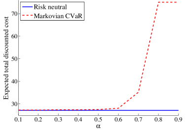
Figure 2: Expected total discounted cost by following risk-neutral and Markovian CVaR policies.

Fig. 3 shows the recursive CVaR value for stationary policies $\pi_{\text{neutral}}^{*}$ and $\pi_{\text{CVaR}}^{*}.$ From Table II, when $\alpha$ is large, $\pi_{\text{CVaR}}^{*}$ prevents the decision maker from keeping the equipment (i.e., $a=\text{K}$), thus reducing the chance of reaching the bad state $s^{\text{bad}}$ and incurring a large cost.

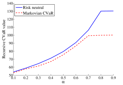
Figure 3: Recursive CVaR value of risk-neutral and Markovian CVaR policies.

VIII Conclusion

In this paper, we have extended simulation-based approximate value iteration algorithms for classical risk-neutral MDPs to the risk-aware setting. This work is significant because it shows that, under mild technical assumptions, risk-aware sequential decision-making can be done efficiently on large scales. Our algorithms apply to the whole class of Markov risk measures, and generalize several recent studies that focused on specific risk measures. Most importantly, we are able to give finite time bounds (instead of asymptotic bounds) in both supremum and $p-$norms on the solution quality of our algorithms so that decision makers may know the quality of the resulting policies as a function of computational effort.

We have two main directions for future work. First, Markov risk measures developed in [3] naturally lead to dynamic programming formulations. Yet, there are still many risk-aware MDPs (e.g., [7]) that do not satisfy the time consistency axiom. We wish to develop simulation-based algorithms for those models as well. Second, we are interested in creating online algorithms for risk-aware MDPs, such as variants of Q-learning (e.g., [2]). This work would have high impact because it would allow controllers of complex systems to manage risk in real time.

The following well known fact will be used throughout our analysis in this paper, we mention it here for ease of reference.

Fact 1

Let $X$ be a given set, and $f_{1}\mbox{ : }X\rightarrow\mathbb{R}$ and $f_{2}\mbox{ : }X\rightarrow\mathbb{R}$ be two real-valued functions on $X$. Then,

1. $|\inf_{x\in X}f_{1}\left(x\right)-\inf_{x\in X}f_{2}\left(x\right)|\leq\sup_{x\in X}|f_{1}\left(x\right)-f_{2}\left(x\right)|$,

2. $|\sup_{x\in X}f_{1}\left(x\right)-\sup_{x\in X}f_{2}\left(x\right)|\leq\sup_{x\in X}|f_{1}\left(x\right)-f_{2}\left(x\right)|$.

For a fixed probability measure $P_{0}$ on $\left(\mathbb{S},\mathcal{B}\left(\mathbb{S}\right)\right)$, we define the space $\mathcal{L}=\mathcal{L}_{\infty}\left(\mathbb{S},\mathcal{B}\left(\mathbb{S}\right),P_{0}\right)$ of essentially bounded measurable mappings on $\mathbb{S}$. The following four properties of coherent risk measures are important throughout our analysis:

1. Convexity: $\rho\left(\lambda X+\left(1-\lambda\right)Y\right)\leq\lambda\rho\left(X\right)+\left(1-\lambda\right)\rho\left(Y\right)$ for all $X,Y\in\mathcal{L}$ and $\lambda\in\left[0,1\right]$.

2. Monotonicity: If $X,Y\in\mathcal{L}$ and $X\leq Y$, then $\rho\left(X\right)\leq\rho\left(Y\right)$.

3. Translation equivariance: If $\alpha\in\mathbb{R}$ and $X\in\mathcal{L}$, then $\rho\left(X+\alpha\right)=\rho\left(X\right)+\alpha$.

4. Positive homogeneity: If $\alpha>0$ and $X\in\mathcal{L}$, then $\rho\left(\alpha X\right)=\alpha\rho\left(X\right)$.

Proof of Lemma 1

Proof:

Fix $\pi\in\Pi$, for any $k\geq 0$ we have

$$0\leq c(s_{0},a_{0})+\rho(\gamma c(s_{1},a_{1})+\rho(\gamma^{2}c(s_{2},a_{2})+\cdots+\gamma^{k}\rho(c(s_{k},a_{k}))))$$

$$\leq c_{\max}+\rho\left(\gamma c_{\max}+\rho\left(\gamma^{2}c_{\max}+\cdots\gamma^{k}\rho\left(c_{\max}\right)\right)\right)$$

$$= c_{\max}\left(1-\gamma^{k}\right)/\left(1-\gamma\right),$$

where the inequalities follows by monotonicity of $\rho$ and the equality follows by translation equivariance. Taking the limit as $k\rightarrow\infty$ gives the desired result. ∎

Proof of Lemma 2

Proof:

For any distribution $\nu\in\mathcal{P}\left(\mathbb{S}\right)$ and a set $B\in\mathcal{B}\left(\mathbb{S}\right)$, we have

$$\nu\,Q^{\pi}\left(B\right) =\int_{\mathbb{S}}Q^{\pi}\left(B|s\right)\nu\left(ds\right)$$

$$=\int_{\mathbb{S}}\left[\int_{B}Q^{\pi}\left(dy|s\right)\right]\nu\left(ds\right)$$

$$=\int_{\mathbb{S}}\left[\int_{B}\frac{dQ^{\pi}}{d\mu}\left(y\right)\mu\left(dy\right)\right]\nu\left(ds\right)$$

$$\leq\int_{\mathbb{S}}\int_{B}C_{\mu}\mu\left(dy\right)\nu\left(ds\right)$$

$$=\int_{B}C_{\mu}\mu\left(dy\right)$$

$$=C_{\mu}\mu\left(B\right),$$

by the definition of $C_{\mu}$ and the condition $\int_{\mathbb{S}}\nu\left(ds\right)=1.$ Now let $\nu=\varrho\,Q^{\pi_{1}}Q^{\pi_{2}}\dots Q^{\pi_{M-1}}$ and $\pi=\pi_{M},$ and we obtain $\varrho\,Q^{\pi_{1}}Q^{\pi_{2}}\dots Q^{\pi_{M}}\leq C_{\mu}\mu$, which implies $c\left(M\right)\leq C_{\mu}.$ ∎

Proof of Lemma 3

Proof:

Given $s\in\mathbb{{S}},$ $a\in\mathbb{A},$ $J\in B\left(\mathbb{S};J_{\max}\right)$, $\varepsilon>0$ and $m\geq 1$.

1. For notation convenience, we let $A=A_{1}-A_{2}$ where

   $$A_{1}=\left\{\mathbb{E}\left[\left(J\left(Y^{s,a}\right)-\mathbb{E}\left[J\left(Y^{s,a}\right)|s\right]\right)^{p}|s\right]\right\}^{1/p},$$

   $$A_{2}=\left\{\frac{1}{m}\sum_{j=1}^{m}\left|J\left(Y_{j}^{s,a}\right)-\frac{1}{m}\sum_{j=1}^{m}J\left(Y_{j}^{s,a}\right)\right|^{p}\right\}^{1/p},$$

   and

   $$B=\mathbb{E}\left[J\left(Y^{s,a}\right)|s\right]-\frac{1}{m}\sum_{j=1}^{m}J\left(Y_{j}^{s,a}\right).$$

   First, we need a technical lemma.

   Lemma 15

   Given $p\in[1,+\infty).$ For $x\geq 0$ and $y\in\left(0,1\right),$ we have

   $$\left(x+y\right)^{p}\leq x^{p}+y\left[(1+x)^{p}-x^{p}\right].$$

   Proof:

   We have

   $$\left(x+y\right)^{p} =x^{p}+C_{n}^{1}x^{p-1}y+C_{n}^{2}x^{p-2}y^{2}+\dots+y^{p}$$

   $$\leq x^{p}+y\left(C_{n}^{1}x^{p-1}+C_{n}^{1}x^{p-2}+\dots+1\right)$$

   $$=x^{p}+y\left[(1+x)^{p}-x^{p}\right].$$

   ∎

   Using Lemma 15, we have

   $$\frac{1}{m}\sum_{j=1}^{m}\left|J\left(Y_{j}^{s,a}\right)-\frac{1}{m}\sum_{j=1}^{m}J\left(Y_{j}^{s,a}\right)\right|^{p}$$

   $$\leq \frac{1}{m}\sum_{j=1}^{m}\left(\left|A_{21}\left(j\right)\right|+\left|B\right|\right)^{p}$$

   $$\leq \frac{1}{m}\sum_{j=1}^{m}\left|A_{21}\left(j\right)\right|^{p}+C\left|B\right|$$

   where $A_{21}(j)=J(Y_{j}^{s,a})-\mathbb{E}[J(Y^{s,a})|s]$ and constant $C\triangleq\left(1+J_{\max}\right)^{p}-J_{\max}^{p}>0.$ We thus obtain $\left|A_{2}^{p}-\frac{1}{m}\sum_{j=1}^{m}\left|A_{21}\left(j\right)\right|^{p}\right|\leq C\left|B\right|.$ Since $\mathbb{P}\left(\left|B\right|<\kappa\right)\geq 1-2\exp[-2m\kappa^{2}/J_{\max}]$ by Hoeffding’s inequality, we have

   $$\mathbb{P}\left(\left|A_{2}^{p}-\frac{1}{m}\sum_{j=1}^{m}|A_{21}(j)|^{p}\right|<C\kappa|s\right)\geq 1-2\exp\left[\frac{-2m\kappa^{2}}{J_{\max}^{2}}\right].$$

   By Hoeffding’s inequality, we have

   $$\mathbb{P}\left(\left|A_{1}^{p}-\frac{1}{m}\sum_{j=1}^{m}\left|A_{21}\left(j\right)\right|^{p}\right|<\kappa|s\right)\geq 1-2\exp\left[\frac{-2m\kappa^{2}}{\left(J_{\max}\right)^{2p}}\right].$$

   By a union bounding argument, we have

   $$\mathbb{P}\left(\left|A_{1}^{p}-A_{2}^{p}\right|<\left(1+C\right)\kappa|s\right)\leq 1-2\left(\exp\left[\frac{-2m\kappa^{2}}{J_{\max}^{2}}\right]+\exp\left[\frac{-2m\kappa^{2}}{\left(J_{\max}\right)^{2p}}\right]\right).$$

   To proceed, we need another technical lemma.

   Lemma 16

   For $x,y\in\mathbb{R},$ $p\in[1,+\infty)$, and let $\max\left\{\left|x\right|,\left|y\right|\right\}=c$ where $c$ is a nonnegative constant. We have

   $$\left|x^{p}-y^{p}\right|=\left|x-y\right|\left|x^{p-1}+x^{p-2}y+\dots+y^{p-1}\right|\leq pc^{p-1}\left|x-y\right|.$$

   Since

   $$\max\big{\{}\big{|}(\|J(Y^{s,a})-\|J(Y^{s,a})\|_{\mu}\|_{p,\mu}^{p})^{1/p}\big{|},\big{|}(\|J(Y^{s,a})-\|J(Y^{s,a})\|_{\hat{\mu}}\|_{p,\hat{\mu}}^{p})^{1/p}\big{|}\big{\}}=J_{\max},$$

   we have

   $$\mathbb{P}\left(\left|A\right|>\frac{\varepsilon}{2b}|s\right)$$

   $$\leq \mathbb{P}\left(\left|A_{1}^{p}-A_{2}^{p}\right|>\frac{\varepsilon}{2bpJ_{\max}^{p-1}}|s\right)$$

   $$\leq 2\big{(}\exp[{(-m\varepsilon^{2})}/{(\sqrt{2}bp\left(1+C\right)J_{\max}^{p})^{2}}]+\exp[{(-m\varepsilon^{2})}/{(\sqrt{2}bp\left(1+C\right)J_{\max}^{2p-1})^{2}}]\big{)},$$

   where the second inequality holds due to Lemma 16. Note that

   $$\mathbb{P}\left(\left|B\right|>\frac{\varepsilon}{2}|s\right)\leq 2\exp\left[\frac{-m\varepsilon^{2}}{\left(\sqrt{2}J_{\max}\right)^{2}}\right].$$

   Denote

   $$\delta_{1}^{m}=2\big{(}\exp[-m\varepsilon^{2}/(\sqrt{2}bp(1+C)J_{\max}^{p})^{2}]+\exp[-m\varepsilon^{2}/(\sqrt{2}bp(1+C)J_{\max}^{2p-1})^{2}]\big{)}$$

   $$\delta_{2}^{m}=2\exp[-m\varepsilon^{2}/(\sqrt{2}J_{\max})^{2}].$$

   We have

   $$\mathbb{P}\left(\left|bA+B\right|>\varepsilon|s\right)$$

   $$\leq \mathbb{P}\left(b\left|A\right|+\left|B\right|>\varepsilon|s\right)$$

   $$\leq \mathbb{P}\left(b\left|A\right|>\frac{\varepsilon}{2}|s\right)+\mathbb{P}\left(\left|B\right|>\frac{\varepsilon}{2}|s\right)$$

   $$\leq \delta_{1}^{m}+\delta_{2}^{m}.$$

2. Let

   $$A=\inf_{\eta\in\left[0,J_{\max}\right]}\eta+\mathbb{E}\left[u\left(J\left(Y^{s,a}\right)-\eta\right)|s\right],$$

   $$B=\inf_{\eta\in\left[0,J_{\max}\right]}\eta+\frac{1}{m}\sum_{j=1}^{m}u\left(J\left(Y_{j}^{s,a}\right)-\eta\right).$$

   Using Fact 1, we have

   $$\left|A-B\right|\leq\sup_{\eta\in\left[0,J_{\max}\right]}|\mathbb{E}\left[u\left(J\left(Y^{s,a}\right)-\eta\right)|s\right]-\frac{1}{m}\sum_{j=1}^{m}u\left(J\left(Y_{j}^{s,a}\right)-\eta\right)|.$$

   By Hoeffding’s inequality, for $\eta\in\left[0,J_{\max}\right],$ we have

   $$\mathbb{P}\bigg{(}\bigg{|}\mathbb{E}[u(J(Y^{s,a})-\eta)|s]-\frac{1}{m}\sum_{j=1}^{m}u(J(Y_{j}^{s,a})-\eta)\bigg{|}>\frac{\varepsilon}{2}|s\bigg{)}$$

   $$\leq 2\exp\left[-m\varepsilon^{2}/\left[\sqrt{2}u\left(J_{\max}\right)\right]^{2}\right].$$

   Since the piecewise linear function $u$ is Lipschitz continuous with the Lipschitz constant equal to $\beta_{2},$ we construct an $\varepsilon/\left(2\beta_{2}\right)-$covering net $\mathcal{N}([0,J_{\max}],\varepsilon/(2\beta_{2}))$ on $[0,J_{\max}]\subseteq\mathbb{R}$. For any $\eta\in\left[0,J_{\max}\right],$ we can find $\eta^{\prime}\in\mathcal{N}([0,J_{\max}],\varepsilon/(2\beta_{2}))$ such that

   $$\frac{1}{m}\left|\sum_{j=1}^{m}u\left(J\left(Y_{j}^{s,a}\right)-\eta\right)-\sum_{j=1}^{m}u\left(J\left(Y_{j}^{s,a}\right)-\eta^{\prime}\right)\right|\leq\frac{\varepsilon}{2}.$$

   Here the inequality follows by the Lipschitz continuity of $u.$ Therefore, we conclude

   $$\mathbb{P}\left(\left|A-B\right|>\varepsilon|s\right)\leq 2\left(1+\frac{4\beta_{2}}{\varepsilon}\right)\exp\left[\frac{-m\varepsilon^{2}}{\left[\sqrt{2}u\left(J_{\max}\right)\right]^{2}}\right].$$

3. Let

   $$A=\inf_{\eta\in\left[0,J_{\max}\right]}\eta+\frac{1}{1-\alpha}\mathbb{E}\left[\left(J\left(Y^{s,a}\right)-\eta\right)_{+}|s\right],$$

   $$B=\inf_{\eta\in\left[0,J_{\max}\right]}\eta+\frac{1}{m\left(1-\alpha\right)}\sum_{j=1}^{m}\left(J\left(Y_{j}^{s,a}\right)-\eta\right)_{+}.$$

   Using Fact 1, we have

   $$\left|A-B\right|\leq\sup_{\eta\in\left[0J_{\max}\right]}\frac{1}{1-\alpha}\bigg{|}\mathbb{E}\left[\left(J\left(Y^{s,a}\right)-\eta\right)_{+}|s\right]-\frac{1}{m}\sum_{j=1}^{m}\left(J\left(Y_{j}^{s,a}\right)-\eta\right)_{+}\bigg{|}.$$

   By Hoeffding’s inequality, for $\eta\in\left[0,J_{\max}\right],$ we have

   $$\quad\mathbb{P}\bigg{(}\frac{1}{1-\alpha}\bigg{|}\mathbb{E}\left[\left(J\left(Y^{s,a}\right)-\eta\right)_{+}|s\right]-\frac{1}{m}\sum_{j=1}^{m}\left(J\left(Y_{j}^{s,a}\right)-\eta\right)_{+}\bigg{|}>\frac{\varepsilon}{2}|s\bigg{)}$$

   $$\leq 2\exp\left[\frac{-m\left(\varepsilon\left(1-\alpha\right)\right)^{2}}{\left(\sqrt{2}\left(2-\alpha\right)J_{\max}\right)^{2}}\right].$$

   Since $\left(x\right)_{+}$ has Lipschitz constant $1,$ we construct an $\varepsilon\left(1-\alpha\right)/2-$covering net

   $$\mathcal{N}\left(\left[0,J_{\max}\right],\varepsilon\left(1-\alpha\right)/2\right)$$

   on $\left[0,J_{\max}\right]\subseteq\mathbb{R}$. For any $\eta\in\left[0,J_{\max}\right],$ we can find $\eta^{\prime}\in\mathcal{N}\left(\left[0,J_{\max}\right],\varepsilon\left(1-\alpha\right)/2\right)$ such that

   $$\quad\frac{\left|\sum_{j=1}^{m}\left(J\left(Y_{j}^{s,a}\right)-\eta\right)_{+}-\sum_{j=1}^{m}\left(J\left(Y_{j}^{s,a}\right)-\eta^{\prime}\right)_{+}\right|}{m\left(1-\alpha\right)}\leq\frac{\varepsilon}{2}.$$

   Therefore, we conclude

   $$\mathbb{P}\left(\left|A-B\right|>\varepsilon|s\right)\leq 2\left(1+\frac{4}{\varepsilon\left(1-\alpha\right)}\right)\exp\left[\frac{-m\left(\varepsilon\left(1-\alpha\right)\right)^{2}}{\left(\sqrt{2}\left(2-\alpha\right)J_{\max}\right)^{2}}\right].$$

∎

Proof of Lemma 4

Proof:

The proof follows the proof of [22, Lemma 1]. Let $\Omega$ denote the sample space underlying the random variables. Let $\varepsilon^{\prime\prime}>0$ be arbitrary and let $f^{*}$ be such that $\|f^{*}-T\widehat{J}_{k}\|_{p,\mu}\leq\inf_{f\in\mathcal{F}}\|f-T\widehat{J}_{k}\|_{p,\mu}+\varepsilon^{\prime\prime}.$ We prove the lemma by showing the sequence of inequalities hold simultaneously on a set of events of measure not smaller than $1-\delta$.

$$\|\widehat{J}_{k+1}-T\widehat{J}_{k}\|_{p,\mu} \leq\|\widehat{J}_{k+1}-T\widehat{J}_{k}\|_{p,\hat{\mu}}+\varepsilon^{\prime}$$ (15)

$$\leq\|\widehat{J}_{k+1}-\widetilde{J}\|_{p,\hat{\mu}}+2\varepsilon^{\prime}$$ (16)

$$\leq\|f^{*}-\widetilde{J}\|_{p,\hat{\mu}}+2\varepsilon^{\prime}$$ (17)

$$\leq\|f^{*}-T\widehat{J}_{k}\|_{p,\hat{\mu}}+3\varepsilon^{\prime}$$ (18)

$$\leq\|f^{*}-T\widehat{J}_{k}\|_{p,\mu}+4\varepsilon^{\prime}$$ (19)

$$=d_{p,\mu}(T\widehat{J}_{k},\mathcal{F})+4\varepsilon^{\prime}+\varepsilon^{\prime\prime}.$$ (20)

It then follows that $\|\widehat{J}_{k+1}-T\widehat{J}_{k}\|_{p,\mu}\leq\inf_{f\in\mathcal{F}}\|f-T\widehat{J}_{k}\|_{p,\mu}+4\varepsilon^{\prime}+\varepsilon^{\prime\prime}$ w.p. at least $1-\delta.$ Since $\varepsilon^{\prime\prime}>0$ is arbitrary, it also true that $\|\widehat{J}_{k+1}-T\widehat{J}_{k}\|_{p,\mu}\leq\inf_{f\in\mathcal{F}}\|f-T\widehat{J}_{k}\|_{p,\mu}+4\varepsilon^{\prime}$ w.p. at least $1-\delta.$ The lemma follows by choosing $\varepsilon^{\prime}=\varepsilon/4.$

First, observe that (17) holds for all functions $f\in\mathcal{F}$ and thus the same inequality holds for $f^{*}\in\mathcal{F},$ too. Therefore, (15) - (19) will hold if (15), (16), (18) and (19) hold w.p. at least $1-\delta^{\prime}$ with $\delta^{\prime}=\delta/4.$ Let

$$W=\max\big{(}\big{|}\|f^{*}-T\widehat{J}_{k}\|_{p,\mu}-\|f^{*}-T\widehat{J}_{k}\|_{p,\hat{\mu}}\big{|},\big{|}\|\widehat{J}_{k+1}-T\widehat{J}_{k}\|_{p,\mu}-\|\widehat{J}_{k+1}-T\widehat{J}_{k}\|_{p,\hat{\mu}}\big{|}\big{)}.$$

Next we show $\mathbb{P}\left(W>\varepsilon^{\prime}\right)\leq\delta^{\prime},$ which implies (15) and (19) hold. Note that for all $\omega\in\Omega,$ $\widehat{J}_{k+1}=\widehat{J}_{k+1}\left(\omega\right)\in\mathcal{F}.$ Hence,

$$\sup_{f\in\mathcal{F}}\left|\|f-T\widehat{J}_{k}\|_{p,\mu}-\|f-T\widehat{J}_{k}\|_{p,\hat{\mu}}\right|\geq\left|\|\widehat{J}_{k+1}-T\widehat{J}_{k}\|_{p,\mu}-\|\widehat{J}_{k+1}-T\widehat{J}_{k}\|_{p,\hat{\mu}}\right|$$

holds point-wise in $\Omega.$ Therefore, the inequality

$$\sup_{f\in\mathcal{F}}\left|\|f-T\widehat{J}_{k}\|_{p,\mu}-\|f-T\widehat{J}_{k}\|_{p,\hat{\mu}}\right|\geq W$$

holds point-wise in $\Omega,$ and hence

$$\mathbb{P}\left(W>\varepsilon^{\prime}\right)\leq\mathbb{P}\left(\sup_{f\in\mathcal{F}}\left|\|f-T\widehat{J}_{k}\|_{p,\mu}-\|f-T\widehat{J}_{k}\|_{p,\hat{\mu}}\right|>\varepsilon^{\prime}\right).$$

We claim that

$$\mathbb{P}\left(\sup_{f\in\mathcal{F}}\left|\|f-T\widehat{J}_{k}\|_{p,\mu}-\|f-T\widehat{J}_{k}\|_{p,\hat{\mu}}\right|>\varepsilon^{\prime}\right)$$

$$\leq \mathbb{P}\left(\sup_{f\in\mathcal{F}}\left|\|f-T\widehat{J}_{k}\|_{p,\mu}^{p}-\|f-T\widehat{J}_{k}\|_{p,\hat{\mu}}^{p}\right|>\left(\varepsilon^{\prime}\right)^{p}\right).$$

For any event $\omega$ such that

$$\sup_{f\in\mathcal{F}}\left|\|f-T\widehat{J}_{k}\|_{p,\mu}-\|f-T\widehat{J}_{k}\|_{p,\hat{\mu}}\right|>\varepsilon^{\prime}.$$

For such event $\omega,$ there exists a function $f^{\prime}\in\mathcal{F}$ such that

$$\left|\|f^{\prime}-T\widehat{J}_{k}\|_{p,\mu}-\|f^{\prime}-T\widehat{J}_{k}\|_{p,\hat{\mu}}\right|>\varepsilon^{\prime}.$$

Pick such function. Assume that $\|f^{\prime}-T\widehat{J}_{k}\|_{p,\hat{\mu}}\leq\|f^{\prime}-T\widehat{J}_{k}\|_{p,\mu}$. We obtain $\|f^{\prime}-T\widehat{J}_{k}\|_{p,\hat{\mu}}+\varepsilon^{\prime}<\|f^{\prime}-T\widehat{J}_{k}\|_{p,\mu}.$ Since $p\geq 1,$ $x^{p}+y^{p}\leq\left(x+y\right)^{p}$ for $x,y\geq 0,$ we have $\|f^{\prime}-T\widehat{J}_{k}\|_{p,\hat{\mu}}^{p}+\left(\varepsilon^{\prime}\right)^{p}\leq(\|f^{\prime}-T\widehat{J}_{k}\|_{p,\hat{\mu}}+\varepsilon^{\prime})^{p}<\|f^{\prime}-T\widehat{J}_{k}\|_{p,\mu}^{p}$ and

$$\left|\|f^{\prime}-T\widehat{J}_{k}\|_{p,\mu}^{p}-\|f^{\prime}-T\widehat{J}_{k}\|_{p,\hat{\mu}}^{p}\right|>\left(\varepsilon^{\prime}\right)^{p}.$$

A similar argument can be developed when $\|f^{\prime}-T\widehat{J}_{k}\|_{p,\hat{\mu}}>\|f^{\prime}-T\widehat{J}_{k}\|_{p,\mu}.$ The claim follows since

$$\bigg{|}\sup_{f\in\mathcal{F}}\|f-T\widehat{J}_{k}\|_{p,\mu}^{p}-\|f-T\widehat{J}_{k}\|_{p,\hat{\mu}}^{p}\bigg{|}\geq\left|\|f^{\prime}-T\widehat{J}_{k}\|_{p,\mu}^{p}-\|f^{\prime}-T\widehat{J}_{k}\|_{p,\hat{\mu}}^{p}\right|.$$

Next, we state a concentration inequality derived due to Pollard.

Theorem 4 (Pollard, 1984)

Let $\mathcal{F}$ be a set of measurable functions $f:\mathcal{X}\rightarrow\left[0,K\right]$ and let $\varepsilon>0,$ $m$ be arbitrary. If $X_{i},$ $i=1,\dots,n$ is i.i.d. sequence taking values in the space $\mathcal{X}$ then

$$\mathbb{P}\left(\sup_{f\in\mathcal{F}}\left|\frac{1}{n}\sum_{i=1}^{n}f\left(X_{i}\right)-\mathbb{E}\left[f\left(X_{1}\right)\right]\right|>\varepsilon\right)\leq 8\mathbb{E}[\mathcal{N}(\varepsilon/8,\mathcal{F}(X^{1:n}))]\exp[-n\varepsilon^{2}/128K^{2}].$$

Now, observe that $\|f-T\widehat{J}_{k}\|_{p,\mu}^{p}=\mathbb{E}[|(f(s_{1})-(TJ)(s_{1}))|^{p}],$ and $\|f-T\widehat{J}_{k}\|_{p,\hat{\mu}}^{p}$ is just the sample average approximation of $\|f-T\widehat{J}_{k}\|_{p,\mu}^{p}.$ Hence, by noting that the covering number associated with $\left\{f-TJ|f\in\mathcal{F}\right\}$ is the same as the covering number of $\mathcal{F}$, we apply Theorem 4 and obtain

$$\mathbb{P}\left(\sup_{f\in\mathcal{F}}\left|\|f-T\widehat{J}_{k}\|_{p,\mu}^{p}-\|f-T\widehat{J}_{k}\|_{p,\hat{\mu}}^{p}\right|>\left(\varepsilon^{\prime}\right)^{p}\right)$$

$$\leq 8\mathbb{E}\left[\mathcal{N}\left(\left(\varepsilon^{\prime}\right)^{p}/8,\mathcal{F}\left(s^{1:n}\right)\right)\right]\exp\left[-\frac{n}{2}\left(\frac{1}{8}\left(\frac{\varepsilon^{\prime}}{2J_{\max}}\right)^{p}\right)^{2}\right].$$

By making the right-hand side upper bounded by $\delta^{\prime}=\delta/4$ we get a lower bound on $n$

$$n>128\left(\frac{8J_{\max}}{\varepsilon}\right)^{2p}\left(\log\left(1/\delta\right)+\log\left(32\mathcal{N}_{0}\left(n\right)\right)\right).$$

Next, we prove inequalities (16) and (18). Let $f$ denote an arbitrary random function such that $f=f\left(s;\omega\right)$ is measurable for each $s_{i}\in{\mathbb{S}}$ and assume that $f$ is uniformly bounded by $J_{\max}.$ By triangle inequality, we have

$$\left|\|f-T\widehat{J}_{k}\|_{p,\hat{\mu}}-\|f-\widetilde{J}\|_{p,\hat{\mu}}\right|\leq\|T\widehat{J}_{k}-\widetilde{J}\|_{p,\hat{\mu}}.$$ (21)

It suffices to show that $\|T\widehat{J}_{k}-\widetilde{J}\|_{p,\hat{\mu}}\leq\varepsilon^{\prime}$ holds w.p. $1-\delta^{\prime}.$ Under Assumption 2, we have

$$\mathbb{P}\left(\left|\rho\left(\widehat{J}_{k}\left(Y^{s_{i},a}\right)\right)-\hat{\rho}_{m}\left(\left\{\widehat{J}_{k}\left(Y_{j}^{s_{i},a}\right)\right\}^{m}_{j=1}\right)\right|>\varepsilon^{\prime}|s^{1:n}\right)\leq\theta\left(\varepsilon^{\prime},m\right),$$

Let $\theta\left(\varepsilon^{\prime},m\right)$ upper bounded by $\delta^{\prime}/\left(n\left|\mathbb{A}\right|\right),$ we get a lower bound on $m.$

Since

$$\left|T\widehat{J}_{k}\left(s_{i}\right)-\widetilde{J}\left(s_{i}\right)\right|\leq\max_{a\in\mathbb{A}}\left|\rho\left(\widehat{J}_{k}\left(Y^{s_{i},a}\right)\right)-\hat{\rho}_{m}\left(\left\{\widehat{J}_{k}\left(Y_{j}^{s_{i},a}\right)\right\}^{m}_{j=1}\right)\right|$$

by Fact 1 1), it follows by a union bounding argument that

$$\mathbb{P}\left(\left|T\widehat{J}_{k}\left(s_{i}\right)-\widetilde{J}\left(s_{i}\right)\right|>\varepsilon^{\prime}\big{|}s^{1:n}\right)\leq\delta^{\prime}/n,$$

and hence another union bounding argument yields

$$\mathbb{P}\left(\max_{i=1,\dots,n}\left|T\widehat{J}_{k}\left(s_{i}\right)-\widetilde{J}\left(s_{i}\right)\right|^{p}>\left(\varepsilon^{\prime}\right)^{p}\big{|}s^{1:n}\right)\leq\delta^{\prime}.$$

Taking the expectation of both sides of this inequality gives

$$\mathbb{P}\left(\max_{i=1,\dots,n}\left|T\widehat{J}_{k}\left(s_{i}\right)-\widetilde{J}\left(s_{i}\right)\right|^{p}>\left(\varepsilon^{\prime}\right)^{p}\right)\leq\delta^{\prime}.$$

Hence,

$$\mathbb{P}\left(\frac{1}{n}\sum_{i=1}^{n}\left|T\widehat{J}_{k}\left(s_{i}\right)-\widetilde{J}\left(s_{i}\right)\right|^{p}>\left(\varepsilon^{\prime}\right)^{p}\right)\leq\delta^{\prime}.$$

Therefore by (21), we have

$$\mathbb{P}\left(\left|\|f-T\widehat{J}_{k}\|_{p,\hat{\mu}}-\|f-\widetilde{J}\|_{p,\hat{\mu}}\right|>\varepsilon^{\prime}\right)\leq\delta^{\prime}.$$

Using this with $f=\widehat{J}_{k+1}$ and $f=f^{*}$ shows that inequalities (16) and (18) each hold w.p. at least $1-\delta^{\prime}$. ∎

Proof of Corollary 1

Proof:

The lower bound for $n$ can be found similarly in the proof of Lemma 4. Let $\varepsilon^{\prime}=\varepsilon/4$ and $\delta^{\prime}=\delta/4.$ In the following, we derive the lower bound for $m$ such that $\|T\widehat{J}_{k}-\widetilde{J}\|_{p,\hat{\mu}}\leq\varepsilon^{\prime}$ holds w.p. $1-\delta^{\prime}.$

1. By Lemma 3 1), we have

   $$\mathbb{P}\left(\left|bA+B\right|>\varepsilon^{\prime}|s^{1:n}\right)$$

   $$\leq \mathbb{P}\left(b\left|A\right|+\left|B\right|>\varepsilon^{\prime}|s^{1:n}\right)$$

   $$\leq \mathbb{P}\left(b\left|A\right|>\frac{\varepsilon^{\prime}}{2}|s^{1:n}\right)+\mathbb{P}\left(\left|B\right|>\frac{\varepsilon^{\prime}}{2}|s^{1:n}\right)$$

   $$\leq \delta_{1}^{m}+\delta_{2}^{m},$$

   where $A=A_{1}-A_{2}$ with

   $$A_{1}=\{\mathbb{E}[\left(J\left(Y^{s_{i},a}\right)-\mathbb{E}\left[J\left(Y^{s_{i},a}\right)|s^{1:n}\right]\right)^{p}|s^{1:n}]\}^{1/p},$$

   $$A_{2}=\left\{\frac{1}{m}\sum_{j=1}^{m}\left|J\left(Y_{j}^{s_{i},a}\right)-\frac{1}{m}\sum_{j=1}^{m}J\left(Y_{j}^{s_{i},a}\right)\right|^{p}\right\}^{1/p},$$

   $$B=\mathbb{E}\left[J\left(Y^{s_{i},a}\right)|s^{1:n}\right]-\frac{1}{m}\sum_{j=1}^{m}J\left(Y_{j}^{s_{i},a}\right),$$

   $$\delta_{1}^{m}=2\big{(}\exp[-m(\varepsilon^{\prime})^{2}/(\sqrt{2}bp(1+C)J_{\max}^{p})^{2}]+\exp[-m(\varepsilon^{\prime})^{2}/(\sqrt{2}bp(1+C)J_{\max}^{2p-1})^{2}]\big{)},$$

   $$\delta_{2}^{m}=2\exp[-m(\varepsilon^{\prime})^{2}/(\sqrt{2}J_{\max})^{2}].$$

   Making $\delta_{1}^{m}+\delta_{2}^{m}$ upper bounded by $\delta^{\prime}/\left(n\left|\mathbb{A}\right|\right),$ we get a lower bound on $m.$ The rest of proof is same as the one for Lemma 4, thus omitted. The proof for mean-semideviation risk function can be developed in a similar way.

2. By Lemma 3 2), we have

   $$\mathbb{P}(\left|A-B\right|> \varepsilon^{\prime}\big{|}s^{1:n})\leq 2\left(1+\frac{4\beta_{2}}{\varepsilon^{\prime}}\right)\exp\left[\frac{-m\left(\varepsilon^{\prime}\right)^{2}}{\left[\sqrt{2}u\left(J_{\max}\right)\right]^{2}}\right],$$

   where

   $$A=\inf_{\eta\in\left[0,J_{\max}\right]}\eta+\mathbb{E}\left[u\left(J\left(Y^{s_{i},a}\right)-\eta\right)|s^{1:n}\right],$$

   $$B=\inf_{\eta\in\left[0,J_{\max}\right]}\eta+\frac{1}{m}\sum_{j=1}^{m}u\left(J\left(Y_{j}^{s_{i},a}\right)-\eta\right).$$

   Making the right hand side upper bounded by $\delta^{\prime}/\left(n\left|\mathbb{A}\right|\right),$ we get a lower bound on $m.$ The rest of proof is same as the one for Lemma 4, thus omitted.

3. By Lemma 3 3), we have

   $$\mathbb{P}(\left|A-B\right|>\varepsilon^{\prime}\big{|}s^{1:n})\leq 2\left(1+\frac{4}{\varepsilon^{\prime}\left(1-\alpha\right)}\right)\exp\left[\frac{-m\left(\varepsilon^{\prime}\left(1-\alpha\right)\right)^{2}}{\left(\sqrt{2}\left(2-\alpha\right)J_{\max}\right)^{2}}\right],$$

   where

   $$A=\inf_{\eta\in\left[0,J_{\max}\right]}\eta+\frac{1}{1-\alpha}\mathbb{E}\left[\left(J\left(Y^{s_{i},a}\right)-\eta\right)_{+}|s^{1:n}\right],$$

   $$B=\inf_{\eta\in\left[0,J_{\max}\right]}\eta+\frac{1}{m\left(1-\alpha\right)}\sum_{j=1}^{m}\left(J\left(Y_{j}^{s_{i},a}\right)-\eta\right)_{+}.$$

   Making the right hand side upper bounded by $\delta^{\prime}/\left(n\left|\mathbb{A}\right|\right),$ we get a lower bound on $m.$ The rest of proof is same as the one for Lemma 4, thus omitted.

∎

Proof of Lemma 5

Proof:

1. For all $s\in\mathbb{S}$, we have

   $$[T^{\pi^{*}}\widehat{J}_{k}]\left(s\right)-[T^{\pi^{*}}J^{*}]\left(s\right)$$

   $$= \,\gamma\max_{\mu\in\mathcal{Q}\left(s,\pi^{*}\left(s\right)\right)}\mathbb{E}_{Y\sim\mu}[\widehat{J}_{k}\left(Y\right)]-\gamma\max_{\mu\in\mathcal{Q}\left(s,\pi^{*}\left(s\right)\right)}\mathbb{E}_{Y\sim\mu}[J^{*}\left(Y\right)]$$

   $$\leq \,\gamma Q^{\pi_{k}}(\widehat{J}_{k}-J^{*}),$$

   where $Q^{\pi_{k}}\mbox{ : }B\left(\mathbb{S};J_{\max}\right)\rightarrow B\left(\mathbb{S};J_{\max}\right)$ is a linear operator such that

   $$Q^{\pi_{k}}(\cdot|s)\in\arg\max_{\mu\in\mathcal{Q}(s,\pi^{*}(s))}\mathbb{E}_{Y\sim\mu}[\widehat{J}_{k}(Y)]$$

   is an element of distributional set $\mathcal{Q}\left(s,\pi^{*}\left(s\right)\right)$ for all $s\in\mathbb{S}.$

2. For all $s\in\mathbb{S}$, we have

   $$[T^{\hat{\pi}_{k}}\widehat{J}_{k}]\left(s\right)-\left[T^{\hat{\pi}_{k}}J^{*}\right]\left(s\right)$$

   $$= \,\gamma\max_{\mu\in\mathcal{Q}\left(s,\hat{\pi}_{k}\left(s\right)\right)}\mathbb{E}_{Y\sim\mu}[\widehat{J}_{k}\left(Y\right)]-\gamma\max_{\mu\in\mathcal{Q}\left(s,\hat{\pi}_{k}\left(s\right)\right)}\mathbb{E}_{Y\sim\mu}[J^{*}\left(Y\right)]$$

   $$\geq \,\gamma Q^{\pi_{k}^{*}}(\widehat{J}_{k}-J^{*}),$$

   where $Q^{\pi_{k}^{*}}\mbox{ : }B\left(\mathbb{S};J_{\max}\right)\rightarrow B\left(\mathbb{S};J_{\max}\right)$ is a linear operator such that

   $$Q^{\pi_{k}^{*}}(\cdot|s)\in\arg\max_{\mu\in\mathcal{Q}(s,\hat{\pi}_{k}(s))}\mathbb{E}_{Y\sim\mu}[J^{*}(Y)]$$

   is an element of distributional set $\mathcal{Q}\left(s,\hat{\pi}_{k}\left(s\right)\right)$ for all $s\in\mathbb{S}.$

∎

Proof of Lemma 6

Proof:

Recall that $\pi^{*}$ is the optimal policy. For $k\geq 0$, we have $T\widehat{J}_{k}\leq T^{\pi^{*}}\widehat{J}_{k}$ and

$$\widehat{J}_{k+1}-J^{*}= T\widehat{J}_{k}-T^{\pi^{*}}\widehat{J}_{k}+T^{\pi^{*}}\widehat{J}_{k}-T^{\pi^{*}}J^{*}-\varepsilon_{k}$$

$$\leq T^{\pi^{*}}\widehat{J}_{k}-T^{\pi^{*}}J^{*}-\varepsilon_{k}$$

By Lemma 5 1), there exists a stochastic kernel $Q^{\pi_{k}}$ such that $T^{\pi^{*}}\widehat{J}_{k}-T^{\pi^{*}}J^{*}\leq\gamma Q^{\pi_{k}}(\widehat{J}_{k}-J^{*})$. Therefore, we have

$$\widehat{J}_{k+1}-J^{*}\leq\gamma Q^{\pi_{k}}(\widehat{J}_{k}-J^{*})-\varepsilon_{k},$$

from which we deduce by induction

$$\widehat{J}_{K}-J^{*}\leq\gamma^{K}(Q^{\pi_{K-1}}Q^{\pi_{K-2}}\dots Q^{\pi_{0}})(\widehat{J}_{0}-J^{*})-\sum_{k=0}^{K-1}\gamma^{K-k-1}\left(Q^{\pi_{k+1}}Q^{\pi_{k+2}}\dots Q^{\pi_{K-1}}\right)\varepsilon_{k}.$$ (22)

From definition of $\widehat{\pi}_{k}$, we have $TJ^{*}=T^{\pi^{*}}J^{*}\leq T^{\widehat{\pi}_{k}}J^{*}$ and

$$\widehat{J}_{k+1}-J^{*} =T^{\widehat{\pi}_{k}}\widehat{J}_{k}-T^{\widehat{\pi}_{k}}J^{*}+T^{\widehat{\pi}_{k}}J^{*}-T^{\pi^{*}}J^{*}-\varepsilon_{k}$$

$$\geq T^{\widehat{\pi}_{k}}\widehat{J}_{k}-T^{\widehat{\pi}_{k}}J^{*}-\varepsilon_{k}.$$

By Lemma 5 2), there is a stochastic kernel $Q^{\pi_{k}^{*}}$ such that $T^{\widehat{\pi}_{k}}J_{k}-T^{\widehat{\pi}_{k}}J^{*}\geq\gamma Q^{\pi_{k}^{*}}(\widehat{J}_{k}-J^{*})$. Therefore,

$$\widehat{J}_{k+1}-J^{*}\geq\gamma Q^{\pi_{k}^{*}}(\widehat{J}_{k}-J^{*})-\varepsilon_{k}.$$

By induction, we obtain

$$\widehat{J}_{K}-J^{*}\geq\gamma^{K}(Q^{\pi_{K-1}^{*}}Q^{\pi_{K-2}^{*}}\dots Q^{\pi_{0}^{*}})(\widehat{J}_{0}-J^{*})-\sum_{k=0}^{K-1}\gamma^{K-k-1}(Q^{\pi_{K-1}^{*}}Q^{\pi_{K-2}^{*}}\dots Q^{\pi_{k+1}^{*}})\varepsilon_{k}.$$ (23)

We observe that $T^{\widehat{\pi}_{K}}\widehat{J}_{K}=T\widehat{J}_{K}\leq T^{\pi^{*}}\widehat{J}_{K}$ by definition of $\hat{\pi}_{K}$ and $T$, and note that $J^{\widehat{\pi}_{K}}=T^{\widehat{\pi}_{K}}J^{\pi_{K}}$ and $TJ^{*}=T^{\pi^{*}}J^{*}=J^{*}$ gives

$$J^{\widehat{\pi}_{K}}-J^{*}$$

$$= T^{\widehat{\pi}_{K}}J^{\widehat{\pi}_{K}}-T^{\widehat{\pi}_{K}}\widehat{J}_{K}+T^{\widehat{\pi}_{K}}\widehat{J}_{K}-T^{\pi^{*}}\widehat{J}_{K}+T^{\pi^{*}}\widehat{J}_{K}-T^{\pi^{*}}J^{*}$$

$$\leq T^{\widehat{\pi}_{K}}J^{\widehat{\pi}_{K}}-T^{\widehat{\pi}_{K}}\widehat{J}_{K}+T^{\pi^{*}}\widehat{J}_{K}-T^{\pi^{*}}J^{*}$$

$$\leq \gamma Q^{\hat{\pi}_{K}}(J^{\widehat{\pi}_{K}}-\widehat{J}_{K})+\gamma Q^{\pi_{K}}(\widehat{J}_{K}-J^{*})$$

$$= \gamma Q^{\hat{\pi}_{K}}(J^{\widehat{\pi}_{K}}-J^{*}+J^{*}-\widehat{J}_{K})+\gamma Q^{\pi_{K}}(\widehat{J}_{K}-J^{*}),$$

where $Q^{\hat{\pi}_{K}}\mbox{ : }B\left(\mathbb{S};J_{\max}\right)\rightarrow B\left(\mathbb{S};J_{\max}\right)$ is a stochastic kernel such that

$$Q^{\hat{\pi}_{K}}(\cdot|s)\in\arg\max_{\mu\in\mathcal{Q}(s,\hat{\pi}_{K}(s))}\mathbb{E}_{Y\sim\mu}[J^{\widehat{\pi}_{K}}(Y)]$$

is an element of the distributional set $\mathcal{Q}\left(s,\hat{\pi}_{k}\left(s\right)\right)$ for all $s\in\mathbb{S},$ and the second inequality is by Lemma 5. We then have

$$(I-\gamma Q^{\hat{\pi}_{K}})(J^{\widehat{\pi}_{K}}-J^{*})\leq\gamma(Q^{\pi_{K}}-Q^{\hat{\pi}_{K}})(\widehat{J}_{K}-J^{*}).$$

Note that $(I-\gamma Q^{\hat{\pi}_{K}})$ is invertible and its inverse is a monotonic operator, and we have

$$J^{\widehat{\pi}_{K}}-J^{*}\leq\gamma(I-\gamma Q^{\hat{\pi}_{K}})^{-1}(Q^{\pi_{K}}-Q^{\hat{\pi}_{K}})(\widehat{J}_{K}-J^{*}).$$

Using (22) and (23), and that fact that $\max\left\{|a|,|b|\right\}\leq|a|+|b|$, we obtain

$$J^{\widehat{\pi}_{K}}-J^{*}\leq 2(I-\gamma Q^{\hat{\pi}_{K}})^{-1}\left\{\sum_{k=0}^{K-1}\gamma^{K-k}Q_{1}\varepsilon_{k}+\gamma^{K+1}Q_{2}\left(\widehat{J}_{0}-J^{*}\right)\right\}$$

where

$$Q_{1}=(Q^{\pi_{K}}Q^{\pi_{K-1}}\dots Q^{\pi_{k+1}}+Q^{\hat{\pi}_{K}}Q^{\pi_{K-1}^{*}}Q^{\pi_{K-2}^{*}}\dots Q^{\pi_{k+1}^{*}})/2$$

and

$$Q_{2}=(Q^{\pi_{K}}Q^{\pi_{K-1}}\dots Q^{\pi_{0}}+Q^{\hat{\pi}_{K}}Q^{\pi_{K-1}^{*}}Q^{\pi_{K-2}^{*}}\dots Q^{\pi_{0}^{*}})/2.$$

Taking the absolute value of both sides, we obtain the desired bound. ∎

Proof of Lemma 7

Proof:

The proof follows the proof of [22, Lemma 4]. From Lemma 6, we have

$$J^{\widehat{\pi}_{K}}-J^{*}\leq \frac{2\gamma\left(1-\gamma^{K+1}\right)}{\left(1-\gamma\right)^{2}}\left[\sum_{k=0}^{K-1}\alpha_{k}A_{k}\left|\varepsilon_{k}\right|+\alpha_{K}A_{K}|J^{*}-\widehat{J}_{0}|\right],$$

with the positive coefficients

$$\alpha_{k}=\frac{\left(1-\gamma\right)\gamma^{K-k-1}}{1-\gamma^{K+1}},\quad 0\leq k<K,$$

and

$$\alpha_{K}={[\left(1-\gamma\right)\gamma^{K}]}/{(1-\gamma^{K+1})},$$

such that $\sum_{k=0}^{K}\alpha_{k}=1$ and the probability kernels

$$A_{k}=\frac{1-\gamma}{2}(I-\gamma Q^{\hat{\pi}_{K}})^{-1}[Q^{\pi_{K}}Q^{\pi_{K-1}}\dots Q^{\pi_{k+1}}+Q^{\hat{\pi}_{K}}Q^{\pi_{K-1}^{*}}Q^{\pi_{K-2}^{*}}\dots Q^{\pi_{k+1}^{*}}],$$

for $0\leq k<K$ and

$$A_{K}=\frac{1-\gamma}{2}(I-\gamma Q^{\hat{\pi}_{K}})^{-1}[Q^{\pi_{K}}Q^{\pi_{K-1}}\dots Q^{\pi_{0}}+Q^{\hat{\pi}_{K}}Q^{\pi_{K-1}^{*}}Q^{\pi_{K-2}^{*}}\dots Q^{\pi_{0}^{*}}].$$

We have

$$\left\|J^{\widehat{\pi}_{K}}-J^{*}\right\|_{p,\varrho}^{p}$$

$$= \int\varrho\left(ds\right)|J^{\widehat{\pi}_{K}}\left(s\right)-J^{*}\left(s\right)|^{p}$$

$$\leq \left[\frac{2\gamma\left(1-\gamma^{K+1}\right)}{\left(1-\gamma\right)^{2}}\right]^{p}\int\varrho\left(ds\right)\left[\sum_{k=0}^{K-1}\alpha_{k}A_{k}\left|\varepsilon_{k}\right|+\alpha_{K}A_{K}\left|J^{*}-\widehat{J}_{0}\right|\right]^{p}\left(s\right)$$

$$\leq \left[\frac{2\gamma\left(1-\gamma^{K+1}\right)}{\left(1-\gamma\right)^{2}}\right]^{p}\int\varrho\left(ds\right)\left[\sum_{k=0}^{K-1}\alpha_{k}A_{k}\left|\varepsilon_{k}\right|^{p}+\alpha_{K}A_{K}|J^{*}-\widehat{J}_{0}|^{p}\right]\left(s\right),$$

by using two times Jensen’s inequality (since $A_{k}$ are positive linear operators $A_{k}\mathbf{1}=\mathbf{1}$ and convexity of $x\rightarrow\left|x\right|^{p}$). The term $|J^{*}-\widehat{J}_{0}|$ is bounded by $J_{\max}.$ Under Assumption 3, $\rho A_{k}\leq(1-\gamma)\sum_{M\geq 0}\gamma^{M}c\left(M+K-k\right)\mu.$ If the approximation error in all iterations $k=0,\dots,K-1$ falls below the tolerance $\left\|\varepsilon_{k}\right\|_{p,\mu}\leq\varepsilon$, we deduce

$$\left\|J^{\widehat{\pi}_{K}}-J^{*}\right\|_{p,\varrho}^{p}\leq\left[\frac{2\gamma\left(1-\gamma^{K+1}\right)}{\left(1-\gamma\right)^{2}}\right]^{p}[(1-\gamma^{K+1})^{-1}C_{\varrho,\mu}\varepsilon^{p}+\gamma^{K}(1-\gamma)(1-\gamma^{K+1})^{-1}J_{\max}^{p}].$$

There exists $K$ that is linear in $\log\left(1/\eta\right)$ and $\log J_{\max}$ such that $\gamma^{K}\leq[{\eta(1-\gamma)^{2}}/{(2\gamma J_{\max})}]^{p}.$ By this choice of $K,$ the second term is bounded by $\eta^{p}$ and we have

$$\left\|J^{\widehat{\pi}_{K}}-J^{*}\right\|_{p,\varrho}^{p}\leq\left[\frac{2\gamma}{\left(1-\gamma\right)^{2}}\right]^{p}C_{\varrho,\mu}\varepsilon^{p}+\eta^{p}.$$

∎

Proof of Lemma 9

Proof:

We first write $T$ as

$$\left[TJ\right]\left(s\right)=\min_{a\in\mathbb{A}}\left\{c(s,a)+\gamma\max_{\mu\in\mathcal{Q}\left(s,a\right)}\int J\left(y\right)\mu\left(dy\right)\right\},\quad\forall s\in\mathbb{S},$$

where each $\mathcal{Q}\left(s,a\right)\subset\mathcal{P}\left(\mathbb{S}\right)$ via Fenchel duality. For any $s\in\mathbb{S}$, we have

$$\left|\left[TJ_{1}\right]\left(s\right)-\left[TJ_{2}\right]\left(s\right)\right|$$

$$\leq \gamma\max_{a\in\mathbb{A}}\left|\max_{\mu\in\mathcal{Q}\left(s,a\right)}\int J_{1}\left(y\right)\mu\left(dy\right)-\max_{\mu\in\mathcal{Q}\left(s,a\right)}\int J_{2}\left(y\right)\mu\left(dy\right)\right|$$

$$\leq \gamma\max_{a\in\mathbb{A}}\max_{\mu\in\mathcal{Q}\left(s,a\right)}\int|J_{1}\left(y\right)-J_{2}\left(y\right)|\mu\left(dy\right)$$

$$\leq \gamma\|J_{1}-J_{2}\|_{\infty},$$

using Fact 1. ∎

Proof of Lemma 10

Proof:

Since$\|\widehat{T}J-TJ\|_{\infty}\leq\|\widehat{T}J-\widetilde{T}J\|_{\infty}+\|\widetilde{T}J-TJ\|_{\infty},$ we need to bound terms $\|\widehat{T}J-\widetilde{T}J\|_{\infty}$ and $\|\widetilde{T}J-TJ\|_{\infty},$ separately. First, we bound the term $\|\widehat{T}J-\widetilde{T}J\|_{\infty}$ in the following lemma.

Lemma 17

Let $\varepsilon>0.$ Under Assumption 2, we have

$$\mathbb{P}\left(\|\widehat{T}J-\widetilde{T}J\|_{\infty}\leq\frac{\varepsilon}{2}\right)\geq 1-n\left|\mathbb{A}\right|\theta\left(\frac{\varepsilon}{2\gamma},m\right).$$

Proof:

Fix $s\in\mathbb{S}$ and $J\in B\left(\mathbb{S};J_{\max}\right),$ we have

$$\left|[\widetilde{T}J]\left(s\right)-[\text{$\widehat{T}$}J]\left(s\right)\right|$$

$$\leq \left|\min_{a\in\mathbb{A}}\left\{c(s^{\prime},a)+\gamma\rho\left(J\left(Y^{s,a}\right)\right)\right\}-\min_{a\in\mathbb{A}}\left\{c(s^{\prime},a)+\gamma\hat{\rho}_{m}\left(\left\{J\left(Y_{j}^{s,a}\right)\right\}^{m}_{j=1}\right)\right\}\right|$$

$$\leq \gamma\max_{a\in\mathbb{A}}\left|\rho\left(J\left(Y^{s,a}\right)\right)-\hat{\rho}_{m}\left(\left\{J\left(Y_{j}^{s,a}\right)\right\}^{m}_{j=1}\right)\right|.$$

where the first inequality follows from the definition of random operators $\widehat{T}$ and $\widetilde{T}$, and the second inequality is due to Fact 1 1). Under Assumption 2, we get

$$\mathbb{P}\left(\left|\rho\left(J\left(Y^{s,a}\right)\right)-\hat{\rho}_{m}\left(\left\{J\left(Y_{j}^{s,a}\right)\right\}^{m}_{j=1}\right)\right|>\frac{\varepsilon}{2\gamma}\right)\leq\theta\left(\frac{\varepsilon}{2\gamma},m\right).$$

Note that $|\mathcal{S}|=n$ and

$$\max_{s\in\mathbb{S}}\left|[\widetilde{T}J]\left(s\right)-[\text{$\widehat{T}$}J]\left(s\right)\right|=\max_{s^{\prime}\in\mathcal{S}}\left|[\widetilde{T}J]\left(s^{\prime}\right)-[\text{$\widehat{T}$}J]\left(s^{\prime}\right)\right|$$

$\widetilde{T}J$ is piecewise constant on $\left\{B_{s}\right\}_{s\in\mathcal{S}}.$ We then obtain

$$\mathbb{P}\left(\|\widehat{T}J-\widetilde{T}J\|_{\infty}\leq\frac{\varepsilon}{2}\right)\geq 1-n\left|\mathbb{A}\right|\theta\left(\frac{\varepsilon}{2\gamma},m\right)$$

by a union bounding argument. ∎

Next we bound the term $\|\widetilde{T}J-TJ\|_{\infty}.$

Lemma 18

Let $\varepsilon>0.$ Under Assumption 4 and 5, if the $\epsilon-$net $\mathcal{S}$ is chosen such that

$$\epsilon\leq\frac{\varepsilon}{2\left(\kappa_{c}+\gamma\kappa_{\mu}J_{\max}\right)},$$

we have

$$\|\widetilde{T}J-TJ\|_{\infty}\leq\frac{\varepsilon}{2}.$$

Proof:

We first show that $TJ$ is Lipschitz continuous with constant $\kappa_{c}+\gamma\kappa_{\mu}J_{\max}.$ For $s,s^{\prime}\in\mathbb{S}$ and $J\in B\left(\mathbb{S};J_{\max}\right),$ we have

$$\left|\left[TJ\right]\left(s\right)-\left[TJ\right]\left(s^{\prime}\right)\right|$$

$$\leq \max_{a\in\mathbb{A}}\bigg{|}c(s,a)-c(s^{\prime},a)+\gamma\max_{\mu\in\mathcal{Q}\left(s,a\right)}\int J\left(y\right)\mu\left(dy\right)-\gamma\max_{\mu^{{}^{\prime}}\in\mathcal{Q}\left(s^{\prime},a\right)}\int J\left(y\right)\mu^{{}^{\prime}}\left(dy\right)\bigg{|}$$

$$\leq \max_{a\in\mathbb{A}}|c(s,a)-c(s^{\prime},a)|+\gamma\max_{a\in\mathbb{A}}\bigg{|}\max_{\mu\in\mathcal{Q}\left(s,a\right)}\int J\left(y\right)\mu\left(dy\right)-\max_{\mu^{{}^{\prime}}\in\mathcal{Q}\left(s^{\prime},a\right)}\int J\left(y\right)\mu^{{}^{\prime}}\left(dy\right)\bigg{|}$$

$$\leq \kappa_{c}\|s-s^{\prime}\|_{\infty}+\gamma\max_{a\in\mathbb{A}}\int|J\left(y\right)(\mu_{*}\left(dy|s,a\right)-\mu_{*}^{{}^{\prime}}\left(dy|s^{\prime},a\right))|$$

$$\leq \left(\kappa_{c}+\gamma\kappa_{\mu}J_{\max}\right)\|s-s^{\prime}\|_{\infty}.$$

The third inequality holds due to Assumption 4 1), $\mu_{*}\left(y|s,a\right)\in\arg\max_{\mu\in\mathcal{Q}\left(s,a\right)}\int J\left(y\right)\mu\left(dy\right)$ and $\mu_{*}^{{}^{\prime}}\left(y|s^{\prime},a\right)\in\arg\max_{\mu^{{}^{\prime}}\in\mathcal{Q}\left(s^{\prime},a\right)}\int J\left(y\right)\mu^{{}^{\prime}}\left(dy\right).$ The last inequality is true because of Assumption 4 2) and Lemma 1. Recall that $\widetilde{T}J$ is piecewise constant on $\left\{B_{s}\right\}_{s\in\mathcal{S}}.$ Under Assumption 5, we conclude

$$\|\widetilde{T}J-TJ\|_{\infty}\leq\left(\kappa_{c}+\gamma\kappa_{\mu}J_{\max}\right)\epsilon.$$

Upper bounding the RHS by $\varepsilon/2$ yields the result. ∎

Combining Lemmas 17 and 18 gives the desired bound. ∎

Proof of Lemma 11

Proof:

1. First, we claim $\|\widehat{J}_{K}-J^{*}\|_{\infty}\leq\gamma^{K}J_{\max}+\sum_{k=0}^{K-1}\gamma^{K-k-1}\|\varepsilon_{k}\|_{\infty}$ for $K\geq 1.$ When $K=1$, we verify

   $$\|\widehat{J}_{1}-J^{*}\|_{\infty} \leq\|T\widehat{J}_{0}-TJ^{*}+\varepsilon_{0}\|_{\infty}$$

   $$\leq\gamma\|\widehat{J}_{0}-J^{*}\|_{\infty}+\|\varepsilon_{0}\|_{\infty}$$

   $$\leq\gamma J_{\max}+\left\|\varepsilon_{0}\right\|_{\infty}.$$

   by Lemma 9. Assume that the claim holds for $K=t$

   $$\|\widehat{J}_{t}-J^{*}\|_{\infty}\leq\gamma^{t}J_{\max}+\sum_{k=0}^{t-1}\gamma^{t-k-1}\left\|\varepsilon_{k}\right\|_{\infty}.$$

   When $K=t+1,$ by induction, we have

   $$\|\widehat{J}_{t+1}-J^{*}\|_{\infty} \leq\|T\widehat{J}_{t}-TJ^{*}+\varepsilon_{t}\|_{\infty}$$

   $$\leq\gamma\|\widehat{J}_{t}-J^{*}\|_{\infty}+\|\varepsilon_{t}\|_{\infty}$$

   $$\leq\gamma^{t+1}J_{\max}+\sum_{k=0}^{t}\gamma^{t-k}\left\|\varepsilon_{k}\right\|_{\infty}.$$

   Finally, if $\left\|\varepsilon_{k}\right\|_{\infty}\leq\varepsilon$ for all $0\leq k<K,$ we obtain

   $$\|\widehat{J}_{K}-J^{*}\|_{\infty} \leq\gamma^{K}J_{\max}+\sum_{k=0}^{K-1}\gamma^{K-k-1}\varepsilon$$

   $$\leq\gamma^{K}J_{\max}+\frac{\varepsilon}{1-\gamma}.$$

2. From the proof of Lemma 7, under Assumption 3 and if the approximation error in all iterations $k=0,\dots,K-1$ falls below the tolerance $\left\|\varepsilon_{k}\right\|_{p,\mu}\leq\varepsilon$, we deduce

   $$\|J^{\widehat{\pi}_{K}}-J^{*}\|_{p,\varrho}^{p}$$

   $$\leq \left[\frac{2\gamma}{\left(1-\gamma\right)^{2}}\right]^{p}\big{[}(1-\gamma^{K+1})^{p-1}C_{\varrho,\mu}\varepsilon^{p}+\gamma^{K}(1-\gamma)(1-\gamma^{K+1})^{p-1}J_{\max}^{p}\big{]}$$

   $$\leq \left[\frac{2\gamma}{(1-\gamma)^{2}}\right]^{p}\big{[}(C_{\varrho,\mu}^{1/p}\varepsilon)^{p}+(\gamma^{K/p}(1-\gamma)^{1/p}(1-\gamma^{K+1})^{1-1/p}J_{\max})^{p}\big{]}.$$

   The second inequality follows from the fact that $(1-\gamma^{K+1})^{p-1}\leq 1$ for all $K\geq 0$ (since $p\geq 1$). Thus,

   $$\|J^{\widehat{\pi}_{K}}-J^{*}\|_{p,\varrho}\leq\frac{2\gamma}{(1-\gamma)^{2}}[C_{\varrho,\mu}^{1/p}\varepsilon+\gamma^{K/p}(1-\gamma)^{1/p}(1-\gamma^{K+1})^{1-1/p}J_{\max}].$$

∎

Proof Lemma 12

Proof:

Define a random variable

$$\mathfrak{Y}\left(\theta\right)=\begin{cases}\max\left\{\theta-1,1\right\},&\mbox{w.p. }p,\\ K^{*},&\mbox{w.p. }1-p,\end{cases}$$

as a function of $\theta.$ It can be seen that $Y_{k+1}$ has the same distribution as $\left[\mathfrak{Y}\left(\Theta\right)|\Theta=Y_{k}\right].$ Using [49, Theorem 1.A.3(d)] and [49, Theorem 1.A.6], the rest of the proof follows the proof of [24, Theorem 4.1] thus omitted. ∎

Proof of Lemma 13

Proof:

The stationary probabilities $\left\{\mu\left(i\right)\right\}_{i=1}^{K^{*}}$ satisfy the following set of equations

$$\mu\left(1\right)=p\mu\left(1\right)+p\mu\left(2\right),$$ (24)

$$\mu\left(i\right)=p\mu\left(i+1\right),\quad\forall i=2,\dots,K^{*}-1,$$ (25)

$$\sum_{i=1}^{K^{*}}\mu\left(i\right)=1.$$ (26)

From the recursive relation (25), we have

$$\mu\left(i\right)=p^{K^{*}-i}\mu\left(K^{*}\right),\quad\forall i=2,\dots,K^{*}-1,$$

and from (24) we have

$$\mu\left(1\right)=\frac{p}{1-p}\mu\left(2\right)=\frac{p^{K^{*}-1}}{1-p}\mu\left(K^{*}\right).$$

We can solve $\mu\left(K^{*}\right)$ using Equation (26)

$$1 = \sum_{i=1}^{K^{*}}\mu\left(i\right)$$

$$= \frac{p^{K^{*}-1}}{1-p}\mu\left(K^{*}\right)+\sum_{i=2}^{K^{*}}p^{K^{*}-i}\mu\left(K^{*}\right)$$

$$= \left[\frac{p^{K^{*}-1}}{1-p}+\frac{1-p^{K^{*}-1}}{1-p}\right]\mu\left(K^{*}\right)$$

$$= \frac{1}{1-p}\mu\left(K^{*}\right),$$

which implies $\mu\left(K^{*}\right)=1-p.$ Therefore,

$$\mu\left(i\right)=p^{K^{*}-i}\mu\left(K^{*}\right)=\left(1-p\right)p^{K^{*}-i},\quad\forall i=2,\dots,K^{*}-1,$$

and

$$\mu\left(1\right)=p^{K^{*}-1}.$$

∎

Proof of Proposition 1

Proof:

1. From Lemma 12 and 13, and the definition of $p$, we have

   $$\mathbb{P}\left(\|\widehat{J}_{k}-J^{*}\|_{\infty}>\epsilon_{g}\right)\leq \mathcal{\mathcal{Q}}\left(Y>1\right)$$

   $$= 1-\mu\left(1\right)$$

   $$= 1-\left(1-\delta\right)^{K^{*}-1}.$$

   Let the RHS be less than or equal to $\delta_{1},$ and we have $1-\delta_{1}\leq\mu\left(1\right)=\left(1-\delta\right)^{K^{*}-1}\leq 1-\delta.$ Therefore, by Lemma 10, we choose $\varepsilon<\epsilon_{g}.$ Furthermore, $\epsilon$ and $m$ should be selected such that

   $$\epsilon\leq\frac{\varepsilon}{2\left(\kappa_{c}+\gamma\kappa_{\mu}J_{\max}\right)}$$

   and

   $$\theta\left(\frac{\epsilon_{g}}{2\gamma},m\right)\leq\frac{\delta_{1}}{\left|\mathbb{A}\right|\left|\mathcal{S}\right|}.$$

2. From Lemma 12 and 13, and the definition of $p$, we have

   $$\mathbb{P}\left(\|J^{\widehat{\pi}_{k}}-J^{*}\|_{p,\varrho}>\epsilon_{g}\right)\leq\mathcal{\mathcal{Q}}\left(Y>1\right)=1-\mu\left(1\right).$$

   Let the RHS be less than or equal to $\delta_{1},$ and we have $1-\delta_{1}\leq\mu\left(1\right)=\left(1-\delta\right)^{K^{*}-1}\leq 1-\delta.$ Therefore, by Lemma 4, we choose $\varepsilon<\epsilon_{g}-d_{p,\mu}\left(T\mathcal{F},\mathcal{F}\right).$ Furthermore, $n,m$ should be selected such that

   $$n>128\left(\frac{8J_{\max}}{\varepsilon}\right)^{2p}\left(\log\left(1/\delta_{1}\right)+\log\left(32\mathcal{N}_{0}\left(n\right)\right)\right)$$

   where

   $$\mathcal{N}_{0}\left(n\right)=\mathcal{N}\left(\frac{1}{8}\left(\frac{\varepsilon}{4}\right)^{p},\mathcal{F},n,\mu\right)$$

   and

   $$\theta\left(\varepsilon/4,m\right)\leq\frac{\delta_{1}}{4n\left|\mathbb{A}\right|}.$$

∎

Proof of Lemma 14

Proof:

The proof follows that of [24, Lemma 5.1]. The transition matrix $\mathfrak{Q}\in\mathbb{R}^{K^{*}\times K^{*}}$ of the Markov chain $\{Y_{k}\}_{k\geq 0}$ has the form

$$\mathfrak{Q}=\left(\IEEEeqnarraybox*[][c]{,c/c/c/c/c/c,}p&00\dots 01-p\\ p00\dots 01-p\\ 0p0\dots 01-p\\ \vdots\vdots\vdots\ddots\vdots\vdots\\ 000\dots 01-p\\ 0000p1-p\right).$$

We claim the eigenvalues $\lambda$ of $\mathfrak{Q}$ are $0$ and $1$. To see this, suppose $\lambda\neq 0$ and $\mathfrak{Q}x=\lambda x$ for some nonzero $x=\left(x_{1},x_{2},\dots,x_{K^{*}}\right)\in\mathbb{R}^{K^{*}}.$ The first and second equalities of linear system $\mathfrak{Q}x=\lambda x$ are

$$\lambda x_{1}=px_{1}+\left(1-p\right)x_{K^{*}},$$

$$\lambda x_{2}=px_{1}+\left(1-p\right)x_{K^{*}}.$$

This implies $x_{2}=x_{1}.$ The third equality of linear system $\mathfrak{Q}x=\lambda x$ is

$$\lambda x_{3}=px_{2}+\left(1-p\right)x_{K^{*}}=px_{1}+\left(1-p\right)x_{K^{*}}=\lambda x_{2},$$

which implies $x_{3}=x_{2}.$ Continuing this reasoning inductively, we have $x_{1}=x_{2}=\dots=x_{K^{*}}$ for any eigenvector $x$ of $\mathfrak{Q}.$ Therefore, it is true that the eigenvalues $\lambda$ of $\mathfrak{Q}$ are $0$ and $1$. By [50, Theorem 12.3], we have

$$t_{mix}\left(\delta_{2}\right)\leq\log\left(\frac{1}{\delta_{2}\mu_{\min}}\right)\frac{1}{1-\lambda_{*}},$$

where $\lambda_{*}=\max\left\{\left|\lambda\right|:\lambda\,\,\text{is an eigenvalue of }\mathfrak{Q},\,\lambda\neq 1\right\}=0.$ Plugging in $\lambda_{*}$ gives the desired result. ∎

Proof of Proposition 2

Proof:

For

$$k\geq\log\left(\frac{1}{\delta_{2}\mu_{\min}}\right)\geq t_{mix}\left(\delta_{2}\right),$$

we have

$$d\left(k\right)=\frac{1}{2}\sum_{i=1}^{K^{*}}\left|\mathcal{Q}_{k}\left(Y_{k}=i\right)-\mu\left(i\right)\right|\leq\delta_{2},$$

which implies

$$\mathcal{Q}_{k}\left(Y_{k}=1\right)\geq\mu\left(1\right)-2\delta_{2}.$$

Therefore, from Lemma 12, we have

$$\mathbb{P}\left(\|\widehat{J}_{k}-J^{*}\|_{\infty}>\epsilon_{g}\right)\leq \mathcal{Q}_{k}\left(Y_{k}>1\right)$$

$$= 1-\mathcal{Q}_{k}\left(Y_{k}=1\right)$$

$$\leq 1+2\delta_{2}-\mu\left(1\right)$$

and

$$\mathbb{P}\left(\|J^{\widehat{\pi}_{k}}-J^{*}\|_{p,\varrho}>\epsilon_{g}\right)\leq \mathcal{Q}_{k}\left(Y_{k}>1\right)$$

$$= 1-\mathcal{Q}_{k}\left(Y_{k}=1\right)$$

$$\leq 1+2\delta_{2}-\mu\left(1\right).$$

∎

References

- [1] M. L. Puterman, Markov decision processes: discrete stochastic dynamic programming. John Wiley & Sons, 2014.
- [2] D. P. Bertsekas and J. N. Tsitsiklis, “Neuro-dynamic programming,” Athena Scientific, vol. 7, pp. 15–23, 1996.
- [3] A. Ruszczyński, “Risk-averse dynamic programming for Markov decision processes,” Mathematical Programming, vol. 125, no. 2, pp. 235–261, 2010.
- [4] R. A. Howard and J. E. Matheson, “Risk-sensitive Markov decision processes,” Management Science, vol. 18, no. 7, pp. 356–369, 1972.
- [5] H. M. Markowitz, Portfolio Selection: Efficient Diversification of Investments. John Wiley & Sons, 1959, vol. 16.
- [6] R. T. Rockafellar and S. Uryasev, “Optimization of conditional value-at-risk,” Journal of risk, vol. 2, pp. 21–42, 2000.
- [7] N. Bäuerle and U. Rieder, “More risk-sensitive Markov decision processes,” Mathematics of Operations Research, vol. 39, no. 1, pp. 105–120, 2013.
- [8] D. M. Kreps, “Decision problems with expected utility criteria, ii: Stationarity,” Mathematics of Operations Research, vol. 2, no. 3, pp. 266–274, 1977.
- [9] J. A. Filar, L. C. M. Kallenberg, and H.-M. Lee, “Variance-penalized Markov decision processes,” Mathematics of Operations Research, vol. 14, no. 1, pp. 147–161, 1989.
- [10] V. Borkar and R. Jain, “Risk-constrained Markov decision processes,” IEEE Transactions on Automatic Control, vol. 59, no. 9, pp. 2574–2579, 2014.
- [11] Y. Le Tallec, “Robust, risk-sensitive, and data-driven control of Markov decision processes,” Ph.D. dissertation, Massachusetts Institute of Technology, 2007.
- [12] S. Mannor and J. N. Tsitsiklis, “Algorithmic aspects of mean–variance optimization in Markov decision processes,” European Journal of Operational Research, vol. 231, no. 3, pp. 645–653, 2013.
- [13] D. A. Iancu, M. Petrik, and D. Subramanian, “Tight approximations of dynamic risk measures,” Mathematics of Operations Research, vol. 40, no. 3, pp. 655–682, 2015.
- [14] A. Shapiro, “On a time consistency concept in risk averse multistage stochastic programming,” Operations Research Letters, vol. 37, no. 3, pp. 143–147, 2009.
- [15] H. N. Byström, “Extreme value theory and extremely large electricity price changes,” International Review of Economics & Finance, vol. 14, no. 1, pp. 41–55, 2005.
- [16] J. H. Kim and W. B. Powell, “An hour-ahead prediction model for heavy-tailed spot prices,” Energy Economics, vol. 33, no. 6, pp. 1252–1266, 2011.
- [17] D. R. Jiang and W. B. Powell, “Approximate dynamic programming for dynamic quantile-based risk measures,” arXiv preprint arXiv:1509.01920, 2015.
- [18] P. Glasserman and T.-W. Liu, “Rare-event simulation for multistage production-inventory systems,” Management Science, vol. 42, no. 9, pp. 1292–1307, 1996.
- [19] J. Enders, W. B. Powell, and D. Egan, “A dynamic model for the failure replacement of aging high-voltage transformers,” Energy Systems, vol. 1, no. 1, pp. 31–59, 2010.
- [20] W. B. Powell, Approximate Dynamic Programming: Solving the curses of dimensionality. John Wiley & Sons, 2007, vol. 703.
- [21] D. P. de Farias and B. Van Roy, “The linear programming approach to approximate dynamic programming,” Operations research, vol. 51, no. 6, pp. 850–865, 2003.
- [22] R. Munos and C. Szepesvári, “Finite-time bounds for fitted value iteration,” The Journal of Machine Learning Research, vol. 9, pp. 815–857, 2008.
- [23] J. Rust, “Using randomization to break the curse of dimensionality,” Econometrica: Journal of the Econometric Society, pp. 487–516, 1997.
- [24] W. B. Haskell, R. Jain, and D. Kalathil, “Empirical dynamic programming,” Mathematics of Operations Research, vol. 41, no. 2, pp. 402–429, 2016.
- [25] T. Asamov and A. Ruszczyński, “Time-consistent approximations of risk-averse multistage stochastic optimization problems,” Mathematical Programming, pp. 1–35, 2014.
- [26] A. Tamar, Y. Chow, M. Ghavamzadeh, and S. Mannor, “Sequential decision making with coherent risk,” IEEE Transactions on Automatic Control, vol. PP, no. 99, pp. 1–1, 2016.
- [27] M. Petrik and D. Subramanian, “An approximate solution method for large risk-averse Markov decision processes,” in Proceedings of the Twenty-Eighth Conference on Uncertainty in Artificial Intelligence, ser. UAI’12. AUAI Press, 2012, pp. 805–814.
- [28] R. Jain and P. Varaiya, “Simulation-based optimization of Markov decision processes: An empirical process theory approach,” Automatica, vol. 46, no. 8, pp. 1297–1304, 2010.
- [29] P. Artzner, F. Delbaen, J.-M. Eber, and D. Heath, “Coherent measures of risk,” Mathematical finance, vol. 9, no. 3, pp. 203–228, 1999.
- [30] A. Ruszczyński and A. Shapiro, “Conditional risk mappings,” Mathematics of Operations Research, vol. 31, no. 3, pp. 544–561, 2006.
- [31] B. Rudloff, A. Street, and D. M. Valladão, “Time consistency and risk averse dynamic decision models: Definition, interpretation and practical consequences,” European Journal of Operational Research, vol. 234, no. 3, pp. 743–750, 2014.
- [32] A. Ruszczyński and A. Shapiro, “Optimization of convex risk functions,” Mathematics of Operations Research, vol. 31, no. 3, pp. 433–452, 2006.
- [33] R. A. DeVore, “Nonlinear approximation,” Acta numerica, vol. 7, pp. 51–150, 1998.
- [34] W. L. Cooper and B. Rangarajan, “Performance guarantees for empirical Markov decision processes with applications to multiperiod inventory models,” Operations Research, vol. 60, no. 5, pp. 1267–1281, 2012.
- [35] W. Ogryczak and A. Ruszczyński, “From stochastic dominance to mean-risk models: Semideviations as risk measures,” European Journal of Operational Research, vol. 116, no. 1, pp. 33–50, 1999.
- [36] ——, “On consistency of stochastic dominance and mean–semideviation models,” Mathematical Programming, vol. 89, no. 2, pp. 217–232, 2001.
- [37] A. Shapiro, D. Dentcheva et al., Lectures on stochastic programming: modeling and theory. SIAM, 2014, vol. 16.
- [38] H. M. Markowitz, G. P. Todd, and W. F. Sharpe, Mean-variance analysis in portfolio choice and capital markets. John Wiley & Sons, 2000, vol. 66.
- [39] T. R. Bielecki, H. Jin, S. R. Pliska, and X. Y. Zhou, “Continuous-time mean-variance portfolio selection with bankruptcy prohibition,” Mathematical Finance, vol. 15, no. 2, pp. 213–244, 2005.
- [40] O. L. V. Costa, A. C. Maiali, and A. d. C. Pinto, “Sampled control for mean-variance hedging in a jump diffusion financial market,” IEEE Transactions on Automatic Control, vol. 55, no. 7, pp. 1704–1709, 2010.
- [41] G. Yin and X. Y. Zhou, “Markowitz’s mean-variance portfolio selection with regime switching: from discrete-time models to their continuous-time limits,” IEEE Transactions on Automatic Control, vol. 49, no. 3, pp. 349–360, 2004.
- [42] A. Ben-Tal and M. Teboulle, “An old-new concept of convex risk measures: The optimized certainty equivalent,” Mathematical Finance, vol. 17, no. 3, pp. 449–476, 2007.
- [43] ——, “Expected utility, penalty functions, and duality in stochastic nonlinear programming,” Management Science, vol. 32, no. 11, pp. 1445–1466, 1986.
- [44] ——, “Portfolio theory for the recourse certainty equivalent maximizing investor,” Annals of Operations Research, vol. 31, no. 1, pp. 479–499, 1991.
- [45] A. Ben-Israel and A. Ben-Tal, “Duality and equilibrium prices in economics of uncertainty,” Mathematical Methods of Operations Research, vol. 46, no. 1, pp. 51–85, 1997.
- [46] A. Ben-Tal and A. Ben-Israel, “A recourse certainty equivalent for decisions under uncertainty,” Annals of Operations Research, vol. 30, no. 1, pp. 1–44, 1991.
- [47] P. Artzner, F. Delbaen, J.-M. Eber, and D. Heath, “Coherent measures of risk,” Mathematical Finance, vol. 9, no. 3, pp. 203–228, 1999.
- [48] S. Uryasev, S. Sarykalin, G. Serraino, and K. Kalinchenko, “VaR vs CVaR in risk management and optimization,” in CARISMA conference, 2010.
- [49] M. Shaked and J. G. Shanthikumar, Stochastic Orders. Springer, 2007.
- [50] D. A. Levin, Y. Peres, and E. L. Wilmer, Markov chains and mixing times. American Mathematical Soc., 2009.