Autoencoder Regularized Network For Driving Style Representation Learning

Abstract

In this paper, we study learning generalized driving style representations from automobile GPS trip data. We propose a novel Autoencoder Regularized deep neural Network (ARNet) and a trip encoding framework trip2vec to learn drivers’ driving styles directly from GPS records, by combining supervised and unsupervised feature learning in a unified architecture. Experiments on a challenging driver number estimation problem and the driver identification problem show that ARNet can learn a good generalized driving style representation: It significantly outperforms existing methods and alternative architectures by reaching the least estimation error on average (0.68, less than one driver) and the highest identification accuracy (by at least 3% improvement) compared with traditional supervised learning methods.

1 Introduction

Studying human drivers’ driving behaviors from automobile sensor data is an interesting research topic. Similar to biometrics such as gait, voice, and typing rhythm, each driver also has a signature pattern of driving, which is also called driving style Lin et al. (2014). There are many aspects that can be used to measure driving styles. In this paper, we focus on studying vehicle movement measures including speed change, turning, and their temporal combinations derived from GPS (Global Positioning System) sensor data that are collected in a short and regular time interval (e.g., 1 second). These measures can reflect drivers’ fine-grained behavioral habits of steering and speed control.

Learning driving style representations from automobile sensor data has been intensively studied Van Ly et al. (2013); Lin et al. (2014); Kuderer et al. (2015); Dong et al. (2016). Compared with other automobile sensors, such as OBD (On-Board Diagnostic) system, CAN (Controller Area Network) buses and cameras, GPS sensor data are often easier to collect, making them popular in large-scale research. Auto insurance companies have become highly interested in utilizing driving style information extracted from GPS data to solve their business problems Laurie (2011). A good driving style representation can help answer questions such as if the driver identified on the policy is driving the proper car, how many drivers share a car, and if an additional driver is driving a car, etc. Insights to these questions can be critical for risk evaluation and can be applied to policy premiums in insurance programs such as pay-as-you-drive. Besides, a good driving style representation also helps to better modeling and understanding human drivers’ behaviors, which are beneficial to improving the designs of driving assistance systems, driver-car interactions, and autonomous driving Lin et al. (2014); Kuderer et al. (2015).

Existing approaches typically follow the supervised learning paradigm, where the inputs are vehicle movement features derived from GPS data and the labels are drivers’ identities. The learning process is usually guided by minimizing a classification loss. The driving style representation (features) learnt in this way can work well in describing unseen trips of seen drivers. Nonetheless, the learnt representation is not guaranteed to be a good generalized representation on unseen drivers. When the number of drivers in the training set is small, the learnt model can hardly work well since unseen drivers’ driving behaviors can be extremely diverse in practice. On the other hand, collecting data from a large number of drivers and ensuring a sufficiently large trip training set for each driver can be challenging. Besides, when the number of drivers becomes large (say, thousands), the classifier can become difficult to train.

To solve the problem, in this paper, we propose a novel deep neural network, Autoencoder Regularized Network (ARNet) for generalized driving style representation learning. Figure 1 illustrates the overall architecture. Different from existing deep neural networks, ARNet directly learns from GPS data and combines supervised and unsupervised feature learning in one architecture. The motivation is to use a specially designed autoencoder structure to regularize the discriminative feature learning in a classification network. In ARNet, supervised learning is combined with unsupervised feature reconstruction using a Recurrent Neural Network (RNN) Elman (1990); Chung et al. (2014) output as a shared hidden layer. An $l_{1}$ regularized bottleneck layer (fc1 in Figure 1) of the autoencoder structure serves as the final driving style feature representation extraction layer. The feature learning is guided simultaneously by a classification loss defined on trip labels and a reconstruction loss defined on how well the driving style feature layer reconstructs the hidden RNN output. Notably, the autoencoder in ARNet aims to reconstruct the hidden-layer RNN feature that keep changing in training, but not to reconstruct the fixed network inputs as in typical autoencoder networks. Such a design can be viewed as a form of regularization to the hidden-layer RNN feature for classification: The feature should be discriminative, meanwhile, they should be reconstructible. The bottleneck layer of the autoencoder (fc1) thus can learn the basis of driving styles, which is expected to generalize better on unseen drivers. Reversely, the design can also be regarded as introducing supervisory information to unsupervised feature learning: Labels of limited training samples bring in prior knowledge to the unsupervised autoencoder, making the learnt basis feature more meaningful and discriminative. Furthermore, we also propose a trip encoding framework, namely trip2vec, which encodes a varied-length GPS trip into a fixed-length vector describing the trip-level driving style using the proposed ARNet as the base encoder.

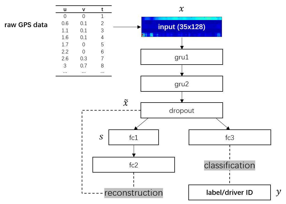
Figure 1: ARNet architecture for driving style representation learning. Dash lines indicate supervisory information.

We study two problems as benchmarks on a large real dataset. The first one is a new and challenging real-world problem raised from the auto insurance industry, called driver number estimation. The objective is to identify the true number of drivers from a set of anonymous trips. Importantly, these drivers are new and unseen to the training phase. Large-scale experimental studies show that ARNet significantly outperforms alternative methods. On a wide range of tests (from 1 to 10 drivers), the average absolute error between the estimation and the ground truth is just 0.68 (less than one driver). In contrast, other candidate methods lead to errors much larger than 1. The second problem is the classical driver identification problem, measured by the classification accuracy on unseen trips of seen drivers. Experiments on a 50-class problem show that, ARNet reaches the highest classification accuracy by at least 3% improvement compared with several existing classification-based methods.

2 Autoencoder Regularized Network (ARNet) And Trip2vec Encoding

We first introduce ARNet that reads GPS data as inputs and learns a compact driving style feature representation. Then, we introduce trip2vec, a trip encoding framework, which extends the learnt driving style representation to trip-level.

2.1 GPS Data Transformation

A trip (i.e., GPS trajectory) can be defined by a varied-length sequence of tuples ($u,v,t$), where ($u,v$) denotes a geo-location and $t$ denotes time. We follow the data transformation method proposed by Dong et al. (2016) to construct neural network inputs from raw GPS data, which has been proved an effective way of extending deep learning to working on GPS data. A trip is first windowed into segments of a fixed length $L_{s}$ with a shift $L_{s}/2$, each of which encodes five instantaneous car movement features, namely basic features, derived from neighboring GPS data: speed norm, difference of speed norm, acceleration norm, difference of acceleration norm, and angular speed. Then, each segment is further applied a sliding window of length $L_{f}$ ($L_{f}<L_{s}$) with a shift $L_{f}/2$. Each window produces a frame encoding seven statistics of the basic features: mean, minimum, maximum, 25%, 50% and 75% quartiles, and standard deviation. As a result, a set of statistical feature matrices of $5\times 7=35$ rows and $2\times L_{s}/L_{f}$ columns can be obtained from a given trip. A feature matrix describing one trip segment defines an input sample to neural networks. For instance, given GPS data sampled once per second as in the experiments, using $L_{s}=256s,L_{f}=4s$, we define feature matrices of size $35\times 128$ as network inputs. The label of a sample inherits from the trip to which the corresponding segment belongs.

2.2 Autoencoder Regularized Network (ARNet)

The proposed ARNet architecture is depicted in Figure 1, which consists of three parts: a stacked RNN, an autoencoder for reconstruction, and a softmax for classification.

2.2.1 Stacked RNN

Let $x$ denote the $35\times 128$ input, i.e., a trip segment. A stacked RNN (gru1+gru2+dropout in Figure 1) reads $x$ to extract higher-level features. As driving style is typically the temporal combination of driving actions, we regard $x$ as a sequence of length 128 and each element of which as a 35-d vector. Here we employs a 2-layer stacked GRU (Gated Recurrent Unit) Cho et al. (2014) architecture to exploit the sequential dependencies. GRU network has been proved an effective RNN design Chung et al. (2014). Our empirical studies show that GRU works slightly better than several popular RNN architectures on our problem, including LSTM Hochreiter and Schmidhuber (1997) and bi-directional RNN Schuster and Paliwal (1997), hence we adopt GRU in the design. The first GRU layer (gru1) reads $35\times 128$ input $x$ with unrolling itself 128 steps along the time axis, and outputs a sequence of a same length 128, each element of which is a vector. The size of the vector (i.e., dimension) equals to the number of hidden units in gru1. The second GRU layer (gru2) is appended to gru1. It also unrolls 128 steps, but outputs a vector instead of a sequence. The size of the vector equals to the number of hidden units in gru2. A dropout layer is applied to gru2 to reduce overfitting Hinton et al. (2012). This dropout layer plays as the shared hidden feature layer bridging the supervised and unsupervised learning. Let $\tilde{x}$ denote its output given an input $x$.

2.2.2 Autoencoder

A 3-layer autoencoder (dropout+fc1+fc2 in Figure 1) is employed for feature reconstruction. Notably, we use the autoencoder to reconstruct $\tilde{x}$ instead of $x$, which is critical for learning better generalized driving style representation. A fully-connected bottleneck layer (fc1) is used to learn a compressed representation $s$ of $\tilde{x}$. ReLU nonlinearity $f(z)=\max(0,z)$ is used in fc1 to ensure $s$ non-negative, which will be used in the trip2vec encoding (see Eq (6)). $l_{1}$ sparsity regularization is applied on $s$ (see Eq (1)). A fully-connected layer (fc2) is the output layer of the autoencoder, where $f(z)=\tanh(z)$ activations are used to approximate $\tilde{x}$ for reconstruction.

2.2.3 Softmax Regression

A fully-connected layer (fc3 in Figure 1) appending to the dropout layer is defined for classification. A softmax regression is applied to produce a distribution over class labels. The number of classes (denoted by $c$) equals to the number of drivers in the training set.

2.2.4 Objective Function and Approximation

Given a training set $\{x_{i},y_{i}\}$ where $i\in\{1,\ldots,n\},y_{i}\in\{1,\ldots,c\}$, the overall objective function is defined as a combination of reconstruction and classification objectives. The reconstruction loss is defined as:

$$\mathcal{J}_{r}=\sum_{i}^{n}||\mathcal{D}s_{i}-\tilde{x}_{i}||_{2}^{2}+\lambda||s_{i}||_{1}\vspace{-0.05in}$$ (1)

where $\tilde{x}_{i}$ is the output of the RNN dropout layer, $\mathcal{D}\in\mathcal{R}^{(n\times k)}$ is a “dictionary” of $k$ vectors, $s_{i}\in\mathcal{R}^{k}$ is a “code vector” associated with the $\tilde{x}_{i}$. The first term of $\mathcal{J}_{r}$ is the reconstruction error, which intends to find a dictionary $\mathcal{D}$ and a new representation $s_{i}$ to reconstruct $\tilde{x}_{i}$, the learnt feature from RNN. $l_{1}$ regularization is used to encourage $s_{i}$ to be sparse. Eq (1) is a sparse coding objective Olshausen and others (1996). The classification loss is defined as the standard cross-entropy:

$$\mathcal{J}_{c}=-\frac{1}{n}\sum_{i}^{n}\sum_{j}^{c}1\{y_{i}=j\}\log\frac{e^{\theta_{j}^{T}\tilde{x}_{i}}}{\sum_{l}^{c}e^{\theta_{l}^{T}\tilde{x}_{i}}}\vspace{-0.05in}$$ (2)

where $1\{\cdot\}$ is the indicator function and $\theta=\{\theta_{1},\ldots,\theta_{c}\}$ are the softmax regression parameters. Overall, the combined objective function is defined as:

$$\min\mathcal{J}_{r}+\mathcal{J}_{c}$$ (3)

The motivation of Eq (1) is as follows. If excluding the autoencoder layers (fc1+fc2), the network becomes a stacked RNN and $\tilde{x}$ can be used as a feature representation of $x$. In this way, the learning of $\tilde{x}$ is guided only by supervisory information of trip labels (i.e., driver IDs). The dropout can help reduce overfitting, but considering the number of unseen drivers can be extremely large, given limited training data, the learning is still prone to overfit to the seen drivers in the training set. Therefore, $\tilde{x}$ can hardly be a good representation for unseen drivers. As a straightforward extension, we want to learn a representation which has the clustering characteristic and be more compact to have better generalization performance. Minimizing $\mathcal{J}_{r}$ can help to achieve this goal. Let us look at the objective of a classical clustering algorithm, K-means Coates and Ng (2012):

$$\min_{\mu}\sum_{k}(||x_{i}-\mu_{k}||^{2})$$ (4)

which intends to find cluster centroids $u_{k}$ that minimize the distance between data points and the nearest centroid. Equally to Eq (4), K-means can be viewed as a way of reconstructing $x_{i}$ Coates and Ng (2012):

$$\min_{\mathcal{D},s}\sum_{i}(||\mathcal{D}s_{i}-x_{i}||^{2}),\quad s.t.\hskip 3.61371pt||s_{i}||_{0}\leq 1,\forall i$$ (5)

Compare Eq (1) and Eq (5), they optimize the same type of reconstruction objective. The only difference is that Eq (1) allows more than one non-zero entry in each $s_{i}$, enabling a much more accurate representation of each $x_{i}$ while still requiring each $s_{i}$ to be simple. Therefore, minimizing $\mathcal{J}_{r}$ can make the learnt representation have clustering characteristics and be more compact.

To achieve the goal of minimizing Eq (1), in ARNet, we use the layers dropout+fc1+fc2 to approximate so as to make the unified architecture easier to train. Known as the sparse coding objective, Eq (1) intends to learn a sparse reconstruction and an efficient coding for $\tilde{x}_{i}$, which shares the spirit of sparse autoencoders Ng (2011). The dropout+fc1+fc2 is a typical autoencoder structure, and we use $l_{1}$ regularization on the output of fc1 so that the coding for $\tilde{x}_{i}$ is sparse.

We can read ARNet from two perspectives. On one hand, we can view $\mathcal{J}_{r}$ (Eq (1)) as regularization terms if regarding $\mathcal{J}_{c}$ (Eq (2)) as the main loss. The autoencoder structure plays as a regularizer to the classification feature $\tilde{x}$, and should improve classification performance. On the other hand, we can view $\mathcal{J}_{c}$ as a term introducing prior knowledge to the unsupervised feature learning guided by $\mathcal{J}_{r}$. The finally learnt feature $s$ thus should work better than features learnt from purely unsupervised learning. Experimental studies in the next section will verify these from both sides.

2.3 Trip2vec: A Trip Encoding Framework

Once we have trained the ARNet, we can use the layers gru1+gru2+dropout+fc1 as a trip segment encoder. But still, it extracts driving style information only from trip data on segment-level, which can be impacted by local factors such as road shapes and traffic conditions, etc. Therefore, we need a more robust representation that describes trip-level driving styles. In order to do so, we propose a trip encoding framework, called trip2vec, which adopts the Bag-of-Words (BoW) feature construction strategy Fei-Fei and Perona (2005) based on the trained trip segment encoder. Roughly speaking, we can treat a varied-length trip as an “article” and each segment as a “paragraph”. The overall “topic” of an article can be derived from aggregating the paragraph-level information. Similarly, based on the segment-level driving styles, we propose to define the trip-level driving style representation by the normalized sum of all the segment-level feature vectors. Figure 2 illustrates the trip2vec framework. Suppose a trip $tr$ is divided into $q$ segments, and the encoded segment features are $\{s^{tr}_{i}\},i\in\{1,\ldots,q\}$. The trip-level driving style feature representation is defined as:

$$S^{tr}=\frac{\sigma^{tr}}{\max_{j}\{\sigma_{j}^{tr}\}}$$ (6)

where $\sigma^{tr}=\sum_{i}^{q}s^{tr}_{i}$ is the vector sum, and $\sigma_{j}^{tr}$ denotes its $j$-th dimension ($\sigma_{j}^{tr}>=0,\forall tr,j$).

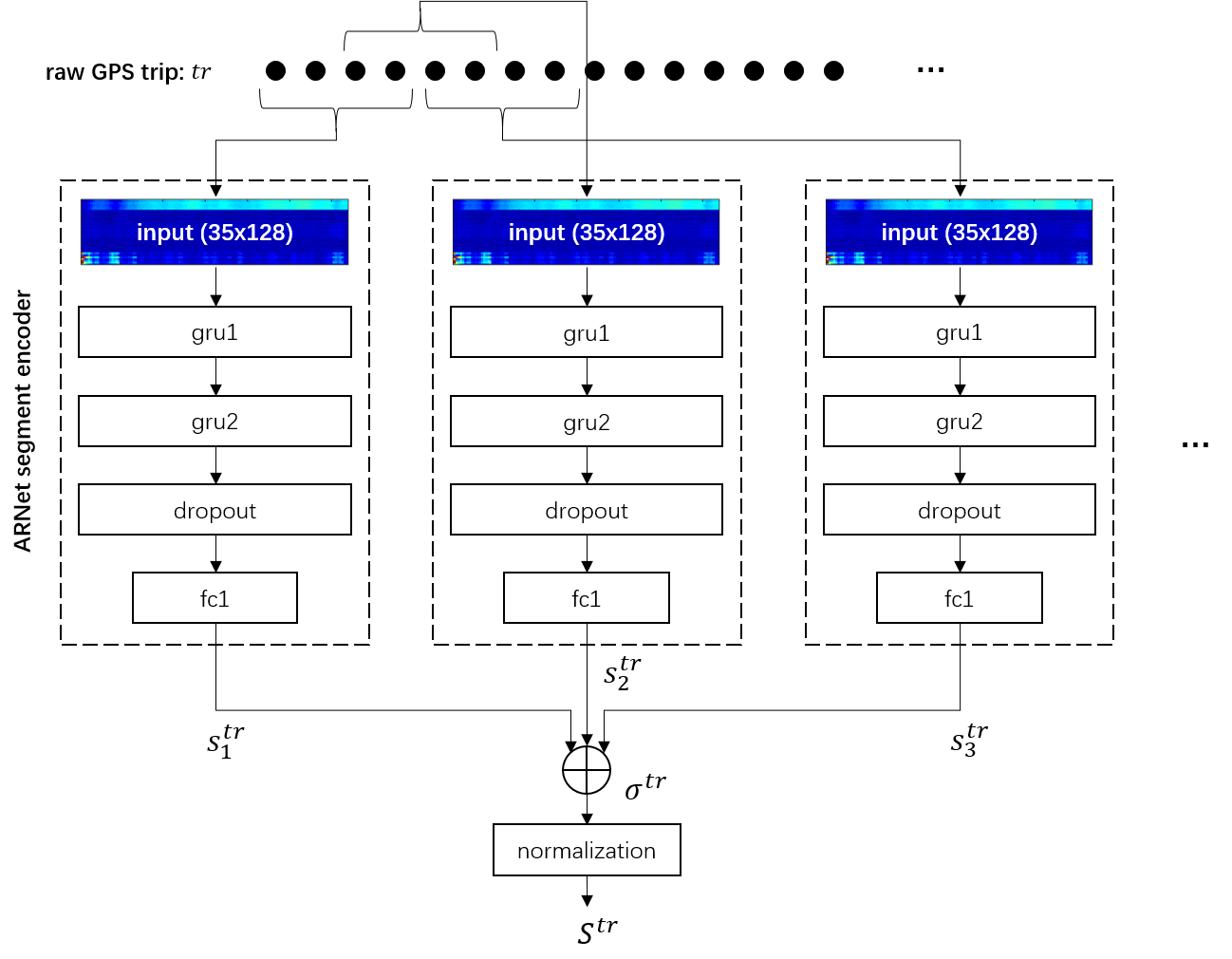
Figure 2: Trip2vec framework

3 Experiments

We use a large real yet private dataset in experiments. The dataset is collected by an insurance company, containing over 500,000 GPS trips from over 2,500 drivers. Each driver has 200 trips that record the car’s location every second.

3.1 Driver Number Estimation Problem

We first study the driver number estimation problem. The aim is to estimate the number of drivers from a set of anonymous trips. The driving style representation learning is based on labeled trips of a set of known drivers, but the testing trips are from unseen new drivers. This is to mimic the situations in real-world, where the auto insurance companies are interested to know how many drivers share a car given this car’s recorded trips. However, the driver ID is unknown for the trips. More importantly, the potential drivers are most likely new, meaning their data are not available in model training, which makes the problem a challenging one. A precise estimation can help improve the risk modeling and pricing policies and to generate direct business values.

3.1.1 Experimental Settings

For comparisons, we include two alternative architectures: a reconstruction-only network (RONet) and a classification-only network (CONet), which are defined by removing one of the two losses from ARNet. For all the nets, we set 256 hidden units in gru1 and gru2, thus dropout output $\tilde{x}$ and fc2 output are both 256-d. We use dropout probability 0.5. We set 50 hidden units in fc1, thus the final driving style representation learnt by ARNet is a 50-d vector. We use $\lambda$=1e-5, ADADELTA optimizer Zeiler (2012) with learning rate 1.0, $\rho$=0.95 and $\epsilon$=1e-8, and batch size 2560 in training these networks. The training is based on the trip data from the first 50 drivers in the dataset. For each driver, we use 80% trips as training data, and the rest 20% as classification validation data. Training ARNet and CONet stops until the validation accuracy is maximized (at epochs 33 and 116, respectively). Training RONet stops when the reconstruction loss $\mathcal{J}_{r}$ converges around 0.001 (at epoch 100). We use fc1 as the driving style feature layer for ARNet and RONet, and use the dropout layer for CONet. Trip features are computed using the proposed trip2vec framework for all the nets.

We also include a 57-d handcrafted trip feature representation proposed by Dong et al. (2016) as another baseline, which demonstrated good classification performance working with GBDT (Gradient Boosting Decision Tree) Friedman (2001). We denote it by TripGBDT feature. The 57 features include global and local driving behavior statistics. The global ones are trip-level statistics of speed, acceleration, and angular speed, total trip time duration, total trip length, trip average speed, and size of the minimal bounding rectangle describing trip geometry. The local ones are statistics of movement features calculated on different time scales with correlation to binned local road shapes. We will compare it with those trip features learnt by the deep architectures.

Based on the trip features, we employ Affinity Propagation (AP) Frey and Dueck (2007) to cluster the trips and estimate the number of drivers. Assuming different drivers should have different driving styles, each obtained cluster refers to the trips belong to one driver, and thus the number of clusters reflects the number of drivers. AP has the advantage of automatically determining the number of clusters. We employ the scikit-learn implementation of AP Pedregosa et al. (2011) using the Euclidean affinity, where a preference parameter is needed. We tuned this parameter for each candidate, and chose preference values -5, -8.5, -12, and -3.5 for ARNet, RONet, CONet, and TripGBDT features, respectively. This is to reduce the effect of clustering algorithm and to fairly compare different feature representations. We use the default damping factor 0.5 in AP, since empirical studies showed that the results are insensitive to this parameter.

3.1.2 Design of Testing

We sample from the unseen drivers (ID greater than 50) who are absent in training to construct testing sets. We build 10 test groups. Each corresponds to a fixed number of drivers, ranging from 1 to 10. For each test group, we randomly sample 25 times from the unseen drivers. As a result, each test group contains 25 trip sets, and each trip set refers to a random combination of drivers. We compute two metrics: (1) the absolute error between the true number of drivers and the estimates, and (2) the AMI (Adjusted Mutual Information) score Vinh et al. (2010) measuring the clustering quality, which returns a value of 1 when the cluster partitions are perfectly matched with the true labels, while random partitions have an expected AMI around 0. For each test group, we report mean and standard deviation of these two metrics on the 25 runs. We also report the overall averaged mean performance across the 10 test groups for each candidate feature representation.

3.1.3 Results

Results are shown in Tables 2 and 2. The best entries in each test group (row) are bolded. We can see that as the number of driver grows, the problem becomes harder. Overall, clustering based on ARNet feature demonstrates the best performance among all. Table 2 shows that ARNet feature leads to the mean error less than one driver in 9 out of the 10 tests. It wins 5 out of the 10 tests with the least mean error, and places the second best in the 5 lost ones all by a small margin (0.12 at most). Its averaged mean error of all the tests is just 0.68. In contrast, the single-loss networks’ features and the TripGBDT feature more often leads to larger errors. They all have the averaged mean error greater than 1. Table 2 shows that ARNet feature also leads to the best clustering quality. It wins 9 (including a tie) of the 10 tests with the highest mean AMI, only with lost the 9-th test by 0.01. Its averaged mean AMI 0.32 is the highest, while other candidates’ are much worse. We depict the box plots of the results in Figures 4 and 4, where A, R, C and T stand for ARNet, RONet, CONet and TripGBDT features, respectively. From the comparisons, we can conclude that the ARNet results are often significantly better. The handcrafted TripGBDT feature performs the worst, implying the superiority of learning representations by deep networks.

Table 1: Driver number estimation: abs. error

# driver	ARNet	RONet	CONet	TripGBDT
1	0.24 $\pm$ 0.43	0.40 $\pm$ 0.49	0.56 $\pm$ 0.50	6.92 $\pm$ 27.4
2	0.48 $\pm$ 0.70	0.76 $\pm$ 0.59	1.12 $\pm$ 0.71	0.44 $\pm$ 0.50
3	0.52 $\pm$ 0.70	0.48 $\pm$ 0.50	1.24 $\pm$ 0.76	0.60 $\pm$ 0.49
4	0.52 $\pm$ 0.57	0.40 $\pm$ 0.50	1.52 $\pm$ 0.90	1.52 $\pm$ 0.50
5	0.48 $\pm$ 0.57	0.40 $\pm$ 0.57	1.72 $\pm$ 1.00	2.32 $\pm$ 0.61
6	0.64 $\pm$ 0.48	0.80 $\pm$ 0.50	1.40 $\pm$ 0.98	3.28 $\pm$ 0.53
7	0.80 $\pm$ 0.63	1.32 $\pm$ 0.61	1.40 $\pm$ 0.89	4.48 $\pm$ 0.50
8	0.72 $\pm$ 0.72	1.52 $\pm$ 0.57	1.52 $\pm$ 1.17	5.40 $\pm$ 0.69
9	0.92 $\pm$ 0.74	2.40 $\pm$ 0.57	1.52 $\pm$ 0.70	50.7 $\pm$ 216∗
10	1.44 $\pm$ 0.75	2.52 $\pm$ 0.75	1.36 $\pm$ 0.84	7.68 $\pm$ 0.55
avg	0.68	1.10	1.34	8.34

^∗Huge outliers exist here, but the samples are not shown in Figure 4 box plot’s scope due to that displaying them in the graph will make the comparisons hard to read at the small scale. # driver ARNet RONet CONet TripGBDT 1 0.76 $\pm$ 0.47 0.60 $\pm$ 0.49 0.44 $\pm$ 0.50 0.12 $\pm$ 0.33 2 0.24 $\pm$ 0.14 0.03 $\pm$ 0.03 0.19 $\pm$ 0.11 0.02 $\pm$ 0.04 3 0.28 $\pm$ 0.14 0.05 $\pm$ 0.03 0.25 $\pm$ 0.12 0.03 $\pm$ 0.04 4 0.31 $\pm$ 0.14 0.04 $\pm$ 0.02 0.29 $\pm$ 0.12 0.02 $\pm$ 0.03 5 0.27 $\pm$ 0.09 0.05 $\pm$ 0.03 0.25 $\pm$ 0.09 0.03 $\pm$ 0.04 6 0.28 $\pm$ 0.07 0.04 $\pm$ 0.02 0.25 $\pm$ 0.07 0.03 $\pm$ 0.04 7 0.27 $\pm$ 0.07 0.05 $\pm$ 0.02 0.25 $\pm$ 0.06 0.02 $\pm$ 0.03 8 0.28 $\pm$ 0.08 0.05 $\pm$ 0.02 0.27 $\pm$ 0.07 0.02 $\pm$ 0.02 9 0.26 $\pm$ 0.05 0.04 $\pm$ 0.01 0.27 $\pm$ 0.05 0.01 $\pm$ 0.02 10 0.27 $\pm$ 0.04 0.05 $\pm$ 0.02 0.27 $\pm$ 0.04 0.01 $\pm$ 0.01 avg 0.32 0.10 0.27 0.03

Table 2: Driver number estimation: AMI score

We studied how the estimation error changes with the AP preference setting, as shown in Figure 5. We can see that the chosen thresholds lead to the best performance for each candidate, revealing that the advantage of ARNet feature is not due to the thresholding of clustering.

We further use t-SNE Maaten and Hinton (2008) to project the trip feature representations onto a 2-d space for visual comparisons. Again, we employ the scikit-learn Pedregosa et al. (2011) t-SNE implementation with all parameters kept default. Figure 6 shows typical results on both seen and unseen drivers. We can see that the ARNet feature is robust: Trips of a same driver show relatively similar driving styles to each other, exhibiting clear clustering patterns, no matter the drivers are seen or unseen. In contrast, due to the absence of supervisory information, RONet learns “too generalized” feature that cannot differentiate drivers well, leading to poor clustering quality (small AMI scores in Table 2). The CONet feature is highly discriminative on seen trips and drivers. Nonetheless, on unseen drivers, it more easily split same-class trips faraway (driver ID 1267 in red color). Similar to RONet result, the TripGBDT feature does not reflect clear clustering patterns, explaining its poor performance. In a word, ARNet learns a better generalized driving style representation, resulting in interpretable better performance on the driver number estimation problem.

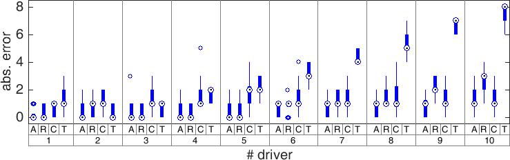
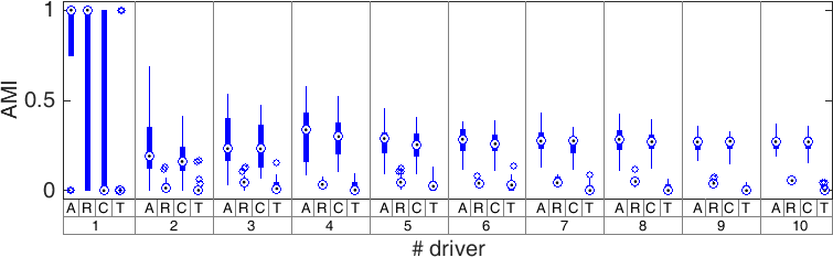
Figure 3: Box plot of abs. error

Figure 4: Box plot of AMI score

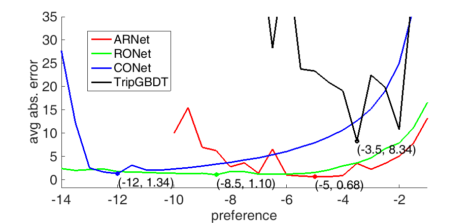
Figure 5: Averaged mean abs. error vs. AP preference. The least-error points are highlighted for each curve.

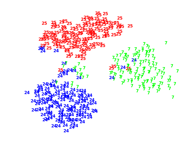
(a) ARNet on seen data

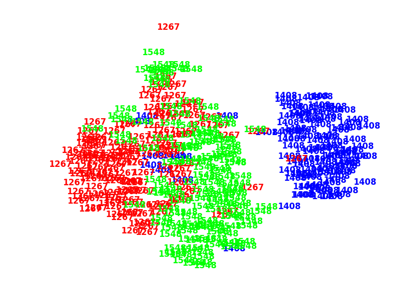
(b) ARNet on unseen data

(c) RONet on seen data

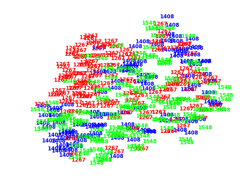
(d) RONet on unseen data

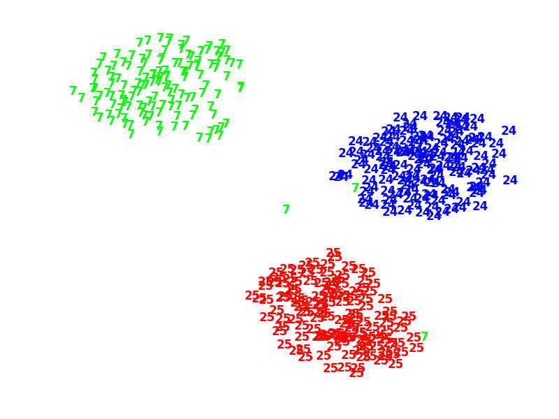
(e) CONet on seen data

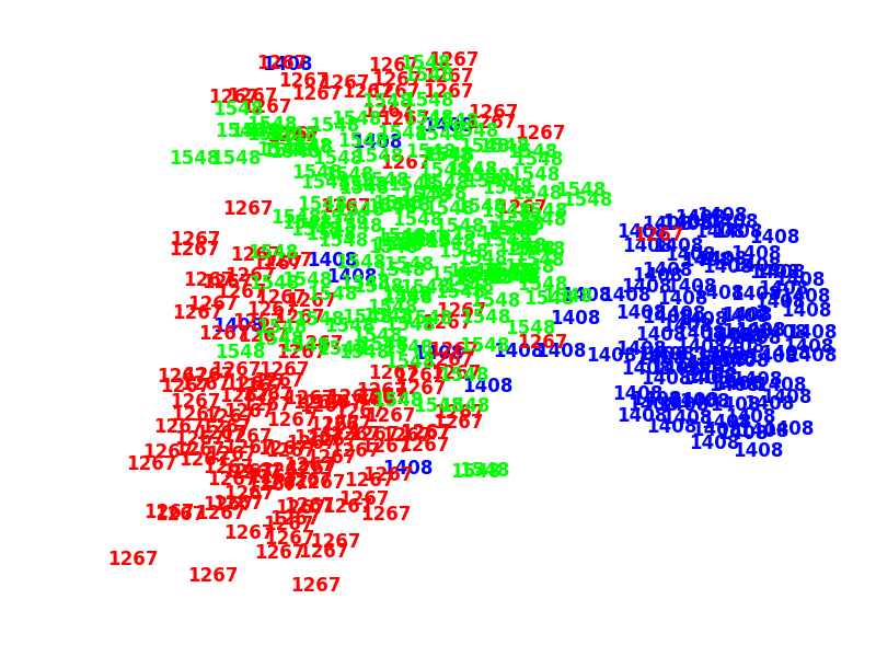
(f) CONet on unseen data

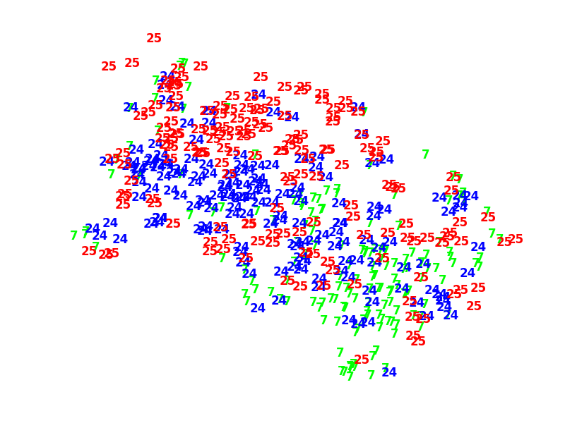
(g) TripGBDT on seen data

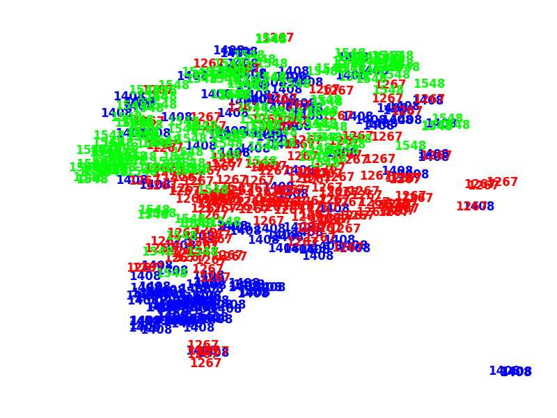
(h) TripGBDT on unseen data

Figure 6: t-SNE projections of trip features, labeled by driver ID. Left column: results on training trips from 3 seen drivers (ID: 7, 24, and 25). Right column: results on trips from 3 unseen drivers (ID: 1267, 1408, and 1548).

3.2 Driver Identification Problem

We now study the classical driver identification problem to demonstrate that ARNet also helps to improve the driver identification (i.e., classification) accuracy. Based on the same 50 drivers used in training on the driver number estimation problem, we train different candidate models and compare both segment-level and trip-level driver classification accuracies (50-class), where the predictions indicate to which driver the segment/trip belongs. A trip-level prediction is obtained by summing up the predictions on segments of this trip to give a vote weighted by the confidence scores. For each driver, we use 80% trips for training and the rest 20% for testing. Note that here the testing trips are all from seen drivers, though the trips are excluded in training.

3.2.1 Candidate Methods

In addition to ARNet and CONet, we compare five different supervised learning deep networks, NoPoolCNN, CNN, PretrainIRNN, IRNN and StackedIRNN studied in Dong et al. (2016) and two GBDT methods, the TripGBDT and a GBDT reading the $35\times 128$ input as a flattened feature vector for learning. ARNet and CONet settings are kept unchanged as in the driver number estimation experiments. In ARNet, the fc3 output is used for prediction.

3.2.2 Results

Table 3: Driver identification accuracy (in %)

method	segment	trip top-1	trip top-5
NoPoolCNN	16.9	28.3	56.7
CNN	21.6	34.9	63.7
PretrainIRNN	28.2	44.6	70.4
IRNN	34.7	49.7	76.9
StackedIRNN	34.8	52.3	77.4
GBDT	18.3	29.1	55.9
TripGBDT	-	51.2	74.3
CONet	37.5	56.1	74.9
ARNet	40.4	58.2	78.3

Table 3 summarizes both segment and trip level accuracies. ARNet outperforms all the other candidates with the highest accuracies, segment 40.4%, trip top-1 58.2%, and trip top-5 78.3%. It improves the accuracies by roughly 3% compared with CONet, which performs the second best in terms of segment and trip top-1 performance. This verifies that ARNet also helps learn a better classification feature representation that improves the supervised learning performance.

4 Related Work

Existing approaches on driving style learning usually follow the supervised learning paradigm, whether or not the input is GPS data. Many methods based on non-deep-learning classifiers and reinforcement learning were proposed, e.g., by López et al. (2012); Quintero M. et al. (2012); Quek and Ng (2013); Van Ly et al. (2013); Kuderer et al. (2015). Recently, Dong et al. (2016) extended deep learning to GPS data and proposed several CNNs and RNNs that can learn interpretable driving style features. But still, these are typical supervised classification networks.

Though in literatures, there are plenty of neural networks combining supervised and unsupervised learning, e.g., Lee and Lin (1992); Karayiannis and Mi (1997); Raina et al. (2007); Collobert and Weston (2008), few attempts were made on employing the autoencoder structure as a special regularizer to supervised learning as in ARNet. Especially, the autoencoder in ARNet is not for pre-training or applying unsupervised/supervised learning in turn, but for guiding the feature learning simultaneously with supervisory signals.

ARNet can also be viewed as a special case of multi-task learning (MTL) if regarding classification and reconstruction as two tasks. However, MTL typically aims to learn a shared representation across tasks Caruana (1997); Argyriou et al. (2007), and in most (if not all) cases, the tasks are either all supervised or all unsupervised. The only MTL method combining unsupervised reconstruction with supervised learning that we are aware of is the Semi-supervised Autoencoder for Multi-task Learning (SAML) Zhuang et al. (2015). In SAML, each task is a combination of reconstruction and classification, and a shared autoencoder reconstructs the network input via shared feature layers used also for classification. Most differently, the autoencoder in ARNet reconstructs the shared hidden-layer feature instead of the network input. Also, the two tasks in ARNet (reconstruction and classification) use different (fc1 and fc3, respectively) but not a shared representation. Besides, SAML is not designed for learning from GPS data. To the best of our knowledge, ARNet is the first attempt on combining unsupervised autoencoder and supervised learning in a unified deep architecture for learning from GPS data.

5 Conclusion

In this paper, we study learning driving style representation from GPS data, and propose a novel deep architecture, Autoencoder Regularized Network (ARNet), which combines unsupervised and supervised feature learning by introducing an autoencoder as a special regularizer to supervised feature learning. ARNet can also be viewed as adding supervisory information to unsupervised feature learning of the autoencoder. In both ways, it improves the quality of learnt driving style representation. We further propose trip2vec, a trip encoding framework using ARNet as the base encoder to extract trip-level driving styles. Experiments on benchmark problems verify the advantages of ARNet over existing methods, especially on characterizing new drivers. Future work includes studying the performance of ARNet on other related problems such as to early detect abnormal driving status (e.g., drunk, fatigue, and drowsy) and those representation learning problems in other domains.

References

- Argyriou et al. [2007] A. Argyriou, T. Evgeniou, and M. Pontil. Multi-task feature learning. Advances in neural information processing systems (NIPS), 19:41–48, 2007.
- Caruana [1997] Rich Caruana. Multitask learning. Mach. Learn., 28(1):41–75, July 1997.
- Cho et al. [2014] Kyunghyun Cho, Bart Van Merriënboer, Dzmitry Bahdanau, and Yoshua Bengio. On the properties of neural machine translation: Encoder-decoder approaches. arXiv preprint arXiv:1409.1259, 2014.
- Chung et al. [2014] Junyoung Chung, Caglar Gulcehre, KyungHyun Cho, and Yoshua Bengio. Empirical evaluation of gated recurrent neural networks on sequence modeling. arXiv preprint arXiv:1412.3555, 2014.
- Coates and Ng [2012] Adam Coates and Andrew Y Ng. Learning feature representations with k-means. In Neural Networks: Tricks of the Trade, pages 561–580. Springer, 2012.
- Collobert and Weston [2008] Ronan Collobert and Jason Weston. A unified architecture for natural language processing: Deep neural networks with multitask learning. In ICML, pages 160–167. ACM, 2008.
- Dong et al. [2016] Weishan Dong, Jian Li, Renjie Yao, Changsheng Li, Ting Yuan, and Lanjun Wang. Characterizing driving styles with deep learning. arXiv preprint arXiv:1607.03611, 2016.
- Elman [1990] Jeffrey L Elman. Finding structure in time. Cognitive science, 14(2):179–211, 1990.
- Fei-Fei and Perona [2005] Li Fei-Fei and Pietro Perona. A bayesian hierarchical model for learning natural scene categories. In CVPR, volume 2, pages 524–531. IEEE, 2005.
- Frey and Dueck [2007] Brendan J. Frey and Delbert Dueck. Clustering by passing messages between data points. Science, 315:972–976, 2007.
- Friedman [2001] Jerome H Friedman. Greedy function approximation: a gradient boosting machine. Annals of statistics, pages 1189–1232, 2001.
- Hinton et al. [2012] Geoffrey E Hinton, Nitish Srivastava, Alex Krizhevsky, Ilya Sutskever, and Ruslan R Salakhutdinov. Improving neural networks by preventing co-adaptation of feature detectors. arXiv preprint arXiv:1207.0580, 2012.
- Hochreiter and Schmidhuber [1997] Sepp Hochreiter and Jürgen Schmidhuber. Long short-term memory. Neural computation, 9(8):1735–1780, 1997.
- Karayiannis and Mi [1997] N. B. Karayiannis and G. W. Mi. Growing radial basis neural networks: merging supervised and unsupervised learning with network growth techniques. IEEE Transactions on Neural Networks, 8(6):1492–1506, Nov 1997.
- Kuderer et al. [2015] Markus Kuderer, Shilpa Gulati, and Wolfram Burgard. Learning driving styles for autonomous vehicles from demonstration. In 2015 IEEE International Conference on Robotics and Automation (ICRA), pages 2641–2646. IEEE, 2015.
- Laurie [2011] Alex Laurie. Telematics: the new auto insurance. Towers Watson, 2011.
- Lee and Lin [1992] C. S. G. Lee and C. T. Lin. Supervised and unsupervised learning with fuzzy similarity for neural-network-based fuzzy logic control systems. In IEEE International Conference on Systems, Man and Cybernetics, pages 688–693 vol.1, 1992.
- Lin et al. [2014] Na Lin, Changfu Zong, Masayoshi Tomizuka, Pan Song, Zexing Zhang, and Gang Li. An overview on study of identification of driver behavior characteristics for automotive control. Mathematical Problems in Engineering, 2014, 2014.
- López et al. [2012] José Oñate López, Andrés C Cuervo Pinilla, et al. Driver behavior classification model based on an intelligent driving diagnosis system. In The 15th International IEEE Conference on Intelligent Transportation Systems, pages 894–899, 2012.
- Maaten and Hinton [2008] Laurens van der Maaten and Geoffrey Hinton. Visualizing data using t-sne. Journal of Machine Learning Research, 9(Nov):2579–2605, 2008.
- Ng [2011] Andrew Ng. Sparse autoencoder. CS294A Lecture notes, 72:1–19, 2011.
- Olshausen and others [1996] Bruno A Olshausen et al. Emergence of simple-cell receptive field properties by learning a sparse code for natural images. Nature, 381(6583):607–609, 1996.
- Pedregosa et al. [2011] F. Pedregosa, G. Varoquaux, A. Gramfort, V. Michel, B. Thirion, O. Grisel, M. Blondel, P. Prettenhofer, R. Weiss, V. Dubourg, J. Vanderplas, A. Passos, D. Cournapeau, M. Brucher, M. Perrot, and E. Duchesnay. Scikit-learn: Machine learning in Python. Journal of Machine Learning Research, 12:2825–2830, 2011.
- Quek and Ng [2013] Zhan Fan Quek and Eldwin Ng. Driver identification by driving style. Technical report, technical report in CS 229 Project, Stanford university, 2013.
- Quintero M. et al. [2012] C. G. Quintero M., José Oñate López, and Andrés C Cuervo Pinilla. Driver behavior classification model based on an intelligent driving diagnosis system. In The 15th International IEEE Conference on Intelligent Transportation Systems, pages 894–899, 2012.
- Raina et al. [2007] Rajat Raina, Alexis Battle, Honglak Lee, Benjamin Packer, and Andrew Y Ng. Self-taught learning: transfer learning from unlabeled data. In ICML, pages 759–766. ACM, 2007.
- Schuster and Paliwal [1997] Mike Schuster and Kuldip K Paliwal. Bidirectional recurrent neural networks. IEEE Transactions on Signal Processing, 45(11):2673–2681, 1997.
- Van Ly et al. [2013] Minh Van Ly, Sujitha Martin, and Mohan M Trivedi. Driver classification and driving style recognition using inertial sensors. In Intelligent Vehicles Symposium (IV), pages 1040–1045. IEEE, 2013.
- Vinh et al. [2010] Nguyen Xuan Vinh, Julien Epps, and James Bailey. Information theoretic measures for clusterings comparison: Variants, properties, normalization and correction for chance. Journal of Machine Learning Research, 11(Oct):2837–2854, 2010.
- Zeiler [2012] Matthew D Zeiler. Adadelta: an adaptive learning rate method. arXiv preprint arXiv:1212.5701, 2012.
- Zhuang et al. [2015] Fuzhen Zhuang, Dan Luo, Xin Jin, Hui Xiong, Ping Luo, and Qing He. Representation learning via semi-supervised autoencoder for multi-task learning. In ICDM, pages 1141–1146. IEEE, 2015.