Textual Entailment with Structured Attentions and Composition

Abstract

Deep learning techniques are increasingly popular in the textual entailment task, overcoming the fragility of traditional discrete models with hard alignments and logics. In particular, the recently proposed attention models [Rocktäschel et al., 2015, Wang and Jiang, 2015] achieves state-of-the-art accuracy by computing soft word alignments between the premise and hypothesis sentences. However, there remains a major limitation: this line of work completely ignores syntax and recursion, which is helpful in many traditional efforts. We show that it is beneficial to extend the attention model to tree nodes between premise and hypothesis. More importantly, this subtree-level attention reveals information about entailment relation. We study the recursive composition of this subtree-level entailment relation, which can be viewed as a soft version of the Natural Logic framework [MacCartney and Manning, 2009]. Experiments show that our structured attention and entailment composition model can correctly identify and infer entailment relations from the bottom up, and bring significant improvements in accuracy.

1 Introduction

Automatically recognizing sentence entailment relations between a pair of sentences has long been believed to be an ideal testbed for discrete approaches using alignments and rigid logic inferences [Zanzotto et al., 2009, MacCartney and Manning, 2009, Wang and Manning, 2010, Watanabe et al., 2012, Tian et al., 2014, Filice et al., 2015]. All of these methods are based on sparse features, making them brittle for unseen phrases and sentences.

Recent advances in deep learning reveal another promising direction to solve this problem. Instead of discrete features and logics, continuous representation of the sentence is more robust to unseen features without sacrificing performance [Bowman et al., 2015]. In particular, the attention model based on LSTM can successfully identify the word-by-word correspondences between the two sentences that lead to entailment or contradiction, which makes the entailment relation inference more focused on local information and less vulnerable to misleading information from other parts of the sentence [Rocktäschel et al., 2015, Wang and Jiang, 2015].

However, conventional neural attention models for entailment recognition problem treat sentences as sequences, ignoring the fact that sentences are formed from the bottom up with syntactic tree structures, which inherently associate with the semantic meanings. Thus, using the tree structure of the sentences will be beneficial in inducing the entailment relations between parts of the two sentences, and then further improving the sentence-level entailment relation classification [Watanabe et al., 2012].

Furthermore, as ?) point out, the entailment relation between sentences is modular, and can be modeled as the composition of subtree-level entailment relations. These subtree-level entailment relations are induced by comparing subtrees between the two sentences, which are by nature a perfect match to be modeled by the attention model over trees.

In this paper we propose a recursive neural network model that calculates the attentions following the tree structures, which helps determine entailment relations between parts of the sentences. We model the entailment relation with a continuous representation.The relation representations of non-leaf nodes are recursively computed by composing their children’s relations. This approach can be viewed as a soft version of Natural Logic [MacCartney and Manning, 2009] for neural models, and can make the recognized entailment relation easier to interpret.

We make the following contributions:

1. We adapt the sequence attention model to the tree structure. This attention model directly works on meaning representations of nodes in the syntactic trees, and provides a more precise guidance for subtree-level entailment relation inference. (Section 2.2)

2. We propose a continuous representation for entailment relation that is specially designed for entailment composition over trees. This entailment relation representation is recursively composed to induce the overall entailment relation, and is easy to interpreted. (Section 2.3)

3. Inspired by the forward and reverse alignment technique in machine translation, we propose dual-attention that considers both the premise-to-hypothesis and hypothesis-to-premise directions, which makes the attention more robust to confusing alignments. (Section 2.4)

4. Experiments show that our model brings significant performance boost based on a Tree-LSTM model. Our dual-attention can provide superior guidance for the entailment relation inference (Figure 4). The entailment composition follows the intuition of Nature Logic and can provide a vivid illustration of how the final entailment conclusion is formed from bottom up (Figure 5). (Section 4)

Figure 1: Exemplary trees for the premise sentence “two women are hugging one another” and the hypothesis sentence “the women are sleeping”. The syntactic labels (NP, VP, CD, etc.) are not used in the model. The dashed and dotted lines show the lowest level of alignments from the hypothesis tree nodes to the premise tree nodes. The blue dashed lines mark the entailment relations, and the red dotted line marks the contradiction relation. In the hypothesis tree, tree nodes in blue squares are identified to be entailment from the premise, and nodes in red squared are identified to contradicts the premise. By composing these relations from the bottom up, we reach a conclusion that the sentence-level entailment relation is contradiction. Please also refer to Figure 5 for real examples taken from our experiments.

2 Structured Attentions & Entailment Composition

Here we first give an overview and formalization of our model, and then describe its components.

2.1 Formalization

We assume both the premise tree and the hypothesis tree are binarized.

We use the premise tree and hypothesis tree in Figure 1 to demonstrate the process of our approach. The premise sentence is “two women are hugging one another”, and the hypothesis sentence is “the women are sleeping”.

Following the traditional approaches [MacCartney and Manning, 2009, Watanabe et al., 2012], we first find the alignments from hypothesis tree nodes to premise tree nodes (i.e., the dashed or dotted curves in Figure 1). Then we explore inducing the sentence-level entailment relations by 1) first computing the entailment relation at each node of the hypothesis tree based on the alignments, and then 2) composing the entailment relations at the internal hypothesis nodes from bottom up to the root in a recursive way. Our model resembles the work of Natural Logic [MacCartney and Manning, 2009] in the spirit that the entailment relation is inferred modularly, and composed recursively.

We formalize this entailment task as a structured prediction problem similar to ?), ?), and ?). The inputs are two trees: premise tree $P$, and hypothesis tree $Q$. The goal is to predict a label $y\in\{\text{contradiction},\text{neutral},\text{entailment}\}$. Note that although the output label $y$ is not structured, we can still consider the problem as a structured prediction problem, because: 1) the input is a pair of trees; and 2) the internal alignments are structured.

More formally, we aim to minimize the negative log likelihood of the gold label given the two trees. The objective can be written in the online fashion as:

$$\ell= -\log\mathrm{Pr}(y|P,Q)=-\log\sum_{\mathbf{A}}\mathrm{Pr}(y,\mathbf{A}|P,Q)$$

$$= -\log\sum_{\mathbf{A}}\mathrm{Pr}(\mathbf{A}|P,Q)\cdot\mathrm{Pr}(y|\mathbf{A},P,Q)=-\log\mathbb{E}_{\mathrm{Pr}(\mathbf{A}|P,Q)}[\mathrm{Pr}(y|\mathbf{A},P,Q)],$$

where the structured latent variable $\mathbf{A}\in\{0,1\}^{|Q|\times|P|}$ represents an alignment. $\lvert\cdot\rvert$ is the number of nodes in the tree. $\mathbf{A}_{ij}=1$ if and only if node $i$ in $Q$ is aligned to node $j$ in $P$, otherwise $\mathbf{A}_{ij}=0$.

However, enumerating over all possible alignments $\mathbf{A}$ takes exponential time, we need to efficiently approximate the above log expectation.

Fortunately, as ?) point out, as long as the calculation $\mathrm{Pr}(y|\mathbf{A},P,Q)$ only consists of linear calculation, simple nonlinearities like $\tanh$, and softmax, we can have following simplification via first-order Taylor approximation:

$$\ell=-\log\mathbb{E}_{\mathrm{Pr}(\mathbf{A}|P,Q)}[\mathrm{Pr}(y|\mathbf{A},P,Q)]\approx-\log\mathrm{Pr}(y|\mathbb{E}_{\mathrm{Pr}(\mathbf{A}|P,Q)}[\mathbf{A}],P,Q)],$$

which means instead of enumerating over all alignments and calculating the label probability for each alignment, we can use the label probability for the expected alignment as an approximation:

$$\tilde{\mathbf{A}}\stackrel{{\scriptstyle\Delta}}{{=}}\mathbb{E}_{\mathrm{Pr}(\mathbf{A}|P,Q)}[\mathbf{A}]\quad\in\mathbb{R}^{\lvert Q\rvert\times\lvert P\rvert}$$ (1)

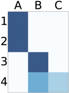
Figure 2(a) shows an example of expected alignment calculation. The objective is simplified to

$$\ell\approx-\log\mathrm{Pr}(y|\tilde{\mathbf{A}},P,Q).$$ (2)

  

$\quad\ \ \ \frac{1}{3}\cdot$ $\quad+\quad\frac{1}{2}\cdot$
$\quad+\quad\frac{1}{6}\cdot$ $\quad=\quad\ \ \$

(a) Expected alignment over 3 alignments with probability distribution of $(\frac{1}{3},\frac{1}{2},\frac{1}{6})$. Each alignment is a matrix of $\{0,1\}^{4\times 4}$, and the expected alignment is a matrix of $\mathbb{R}^{4\times 4}$.

(b) Architecture of our neural network. Layers with the same color share the same parameters. The alignment module calculates the expected alignment $\tilde{\mathbf{A}}$. The Entailment Composition module infers the final entailment $y$.

Figure 2: Expected alignments calculation (a) and overview of the network architecture (b).

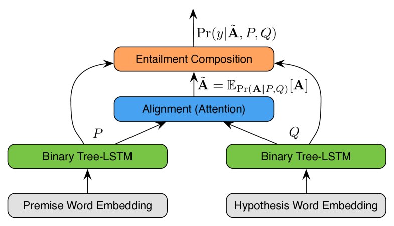
With this observation, we split our calculation into two steps as the top two modules in Figure 2(b). First in the Alignment module, we calculate the expected alignments $\tilde{\mathbf{A}}$ using Equation 1 (Section 2.2). Then we calculate the node-wise entailment relation, propagate and compose the relation from bottom up to find out the final entailment relation (Equation 2) in the Entailment Composition module (Section 2.3). Both of these two modules rely on the composition of tree node meaning representations (Section 3).

2.2 Attention over Tree Nodes

First we calculate the expected alignments $\tilde{\mathbf{A}}$ between the hypothesis $Q$ and the premise $P$ (Equation 1):

$$\tilde{\mathbf{A}}=\mathbb{E}_{\mathrm{Pr}(\mathbf{A}|P,Q)}[\mathbf{A}].$$

To simplify the calculation, we further approximate the global (binary) alignment $\mathbf{A}$ to be consisted of the alignment $\mathbf{A}_{i}\in\{0,1\}^{1\times|P|}$ of each tree node $i\in Q$ independently. $\mathbf{A}_{i}$ is the $i$th row of $\mathbf{A}$:

$$\mathbf{A}=[\mathbf{A}_{1}^{T};\mathbf{A}_{2}^{T};\dots;\mathbf{A}_{\lvert Q\rvert}^{T}]^{T},$$

$$\mathrm{Pr}(\mathbf{A}|P,Q)=\prod_{i}^{\lvert Q\rvert}\mathrm{Pr}(\mathbf{A}_{i}|P,Q).$$

$\mathrm{Pr}(\mathbf{A}_{i,j}=1|P,Q)$ is the probability of the node $i\in Q$ being aligned to node $j\in P$, which is defined as:

$$\mathrm{Pr}(\mathbf{A}_{i,j}=1|P,Q)\stackrel{{\scriptstyle\Delta}}{{=}}\frac{\exp(T_{2k,1}([\mathbf{h}_{i};\mathbf{h}_{j}]))}{\sum_{k}\exp(T_{2k,1}([\mathbf{h}_{i};\mathbf{h}_{k}]))}.$$ (3)

$\mathbf{h}_{i},\mathbf{h}_{j}\in\mathbb{R}^{k}$ are vectors representing the semantic meanings of node $i$, $j$, respectively, whose calculation will be described in Section 3. $T_{2k,1}$ is an affine transformation from $\mathbb{R}^{2k}$ to $\mathbb{R}$. This formulation essentially is equivalent to the widely used attention calculation in neural networks [Bahdanau et al., 2014], i.e., for each node $i\in Q$, we find the relevant nodes $j\in P$ and use the softmax of the relevances as a probability distribution. In the rest of the paper, we use “expected alignment” and “attention” interchangeably.

The expected alignment of node $i$ being aligned to node $j$, by definition, is:

$$\tilde{\mathbf{A}}_{i,j}=\mathrm{Pr}(\mathbf{A}_{i,j}=1|P,Q)\cdot 1=\mathrm{Pr}(\mathbf{A}_{i,j}=1|P,Q).$$

2.3 Entailment Composition

Now we can calculate the entailment relation at each tree node and propagate the entailment relation following the hypothesis tree from bottom up, assuming the expected alignment is given (Equation 2):

$$\ell\approx-\log\mathrm{Pr}(y|\tilde{\mathbf{A}},P,Q).$$

Let vector $\mathbf{e}_{i}\in\mathbb{R}^{r}$ denote the entailment relation in a latent relation space at hypothesis tree node $i\in Q$. At the root of the hypothesis tree. We can induce the final entailment relation from entailment relation vector $\mathbf{e}_{\text{root}}$. We use a simple $\tanh$ layer to project the entailment relation to the 3 relations defined in the task, and use a softmax layer to calculate the probability for each relation:

$$\mathrm{Pr}(y|\tilde{\mathbf{A}},P,Q)=\text{softmax}(\tanh(T_{r,3}(\mathbf{e}_{\text{root}}))).$$

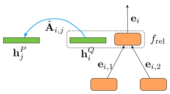
At each hypothesis node $i$, $\mathbf{e}_{i}$ is calculated recursively given the meaning representation at this tree node $\mathbf{h}_{i}$, the meaning representation of every node in the premise tree $\mathbf{h}_{j},j\in P$, and the entailment from $i$’s children, $\mathbf{e}_{i,1},\mathbf{e}_{i,2}$:

$$\mathbf{e}_{i}=f_{\text{rel}}([\mathbf{h}_{i};\sum_{j\in P}\tilde{\mathbf{A}}_{i,j}\mathbf{h}_{j}],\mathbf{e}_{i,1},\mathbf{e}_{i,2})$$ (4)

Figure 3(a) illustrates the calculation of the entailment composition. We will discuss $f_{\text{rel}}$ in Section 3.

(a) Entailment composition at hypothesis tree node $i$. The composition is based on the meaning representation of current node $\mathbf{h}_{i}^{Q}$, the expected alignment for node $i$, $\tilde{\mathbf{A}}_{i}$, expected meaning representation of aligned premise tree node $\sum_{j\in P}\tilde{\mathbf{A}}_{i,j}h_{j}^{P}$, and known entailment relations from children nodes $\mathbf{e}_{i,1},\mathbf{e}_{i,2}$.

$\Bigg{(}$$\Bigg{)}^{\text{T}}\quad\mathbf{\centerdot}\quad$ $\quad=\quad$

(b) An example of dual-attention eliminating uncertainty in the alignment. In the left attention matrix, word “4” can be aligned to either “B” or “C”. In the middle attention matrix, word “C” can be aligned to either “2” or “4”. The element-wise product eliminates these uncertainty and results in the right attention matrix.

  

Figure 3: Entailment composition (a) and dual-attention calculation (b).

2.4 Dual-attention Over Tree Nodes

We can further improve our alignment approximation in Section 2.2, which does not consider any structural information of current tree, nor any alignment information from the premise tree.

We can take a closer look at our conceptual example in Figure 1. Note that the alignments have, to some extent, a symmetric property: if a premise node $j$ is most relevant to a hypothesis node $i$, then the hypothesis node $i$ should also be most relevant to premise node $j$. For example, in Figure 1, the premise phrase “hugging one another” contradicts the hypothesis word “sleeping”. In the perspective of the premise tree, the hypothesis word “sleeping” contradicts by the known claim “hugging one another”. This suggests us to calculate the alignments from both side, and eliminate the unlikely alignment if it only exists in one side. This technique is similar to the widely used forward and reversed alignment technique in the machine translation area.

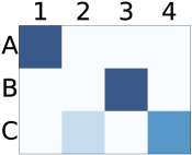
In detail, we calculate the expected alignments $\tilde{\mathbf{A}}$ from hypothesis to premise, and also the expected alignments $\tilde{\mathbf{A}}^{R}$ from premise to hypothesis, and use their element-wise product

$$\tilde{\mathbf{A}}^{*}=\tilde{\mathbf{A}}\cdot\tilde{\mathbf{A}}^{R}$$

as the attention to feed into the Entailment Composition module. This element-wise product is a mimic of the intersection of two alignments in machine translation. Figure 3(b) shows an example.

In addition to our dual-attention, ?) also explore to use the structural information to improve the alignment. However, their approach requires introducing some extra terms in the objective function, and is not straightforward to integrate into our model. We leave adding more structural constraints to further improve the attention as an open problem to explore in the future.

3 Review: Recursive Tree Meaning Representations

Here we describe the final building block of our neural model.

In Section 2.2, we did not mention the calculation of the meaning representation $\mathbf{h}_{i}$ for node $i$ in Equation 3, which represents the semantic meaning of the subtree rooted at node $i$. In general, $\mathbf{h}_{i}$ should be calculated recursively from the meaning representations $\mathbf{h}_{i,1}$, $\mathbf{h}_{i,2}$ of its two children if node $i$ is an internal node, otherwise $\mathbf{h}_{i}$ should be calculated based on the word $\mathbf{x}\in\mathbb{R}^{d}$ in the leaf.

$$\mathbf{h}_{i}=f_{\text{MR}}(\mathbf{x}_{i},\mathbf{h}_{i,1},\mathbf{h}_{i,2}).$$ (5)

Similar is Equation 4, where the relation $\mathbf{e}_{i}$ is recursively calculated from the relation of its two children, as well as the meaning $\mathbf{h}_{i}$ comparing with the meaning of the premise tree:

$$\mathbf{e}_{i}=f_{\text{rel}}([\mathbf{h}_{i};\sum_{j\in P}\tilde{\mathbf{A}}_{i,j}\mathbf{h}_{j}],\mathbf{e}_{i,1},\mathbf{e}_{i,2}).$$ (6)

Note the resemblance between these two equations, which indicates that we can handle them similarly with the same form of composition function $f(\cdot)$.

We have various choices for composition function $f$. For example, we can use simple RNN functions as in ?). Alternatively, we can use a convolutional layer to extract features from $\mathbf{x}_{i},\mathbf{h}_{i,1},\mathbf{h}_{i,2}$ and use pooling as aggregation to form $\mathbf{h}_{i}$. In this paper we choose Tree-LSTM model [Tai et al., 2015]. Our model is independent to this composition function and any high-quality composition function is sufficient for us to infer the meaning representations and entailments.

Here we use Equation 5 as an example. Equation 6 can be handled similarly. Similar to the classical LSTM model [Hochreiter and Schmidhuber, 1997], in the binary Tree-LSTM model of ?), each tree node has a state represented by a pair of vectors: the output vector $\mathbf{h}\in\mathbb{R}^{1\times k}$, and the memory cell $\mathbf{c}\in\mathbb{R}^{1\times k}$, where $k$ is the length of the Tree-LSTM output representation. We use $\mathbf{h}$ as the meaning representation of the tree node in the attention model. The LSTM transition calculates the state $(\mathbf{h}_{i},\mathbf{c}_{i})$ of node $i$ with leaf word $\mathbf{x}_{i}\in\mathbb{R}^{d}$, and two children with states $(\mathbf{h}_{i,1},\mathbf{c}_{i,1})$ and $(\mathbf{h}_{i,2},\mathbf{c}_{i,2})$ respectively.

We can abuse the mathematics a little bit, and write the transition at an LSTM unit as a function:

$$[\mathbf{h}_{i};\mathbf{c}_{i}]=\mathrm{LSTM}(\mathbf{x}_{i},[\mathbf{h}_{i,1};\mathbf{c}_{i,1}],[\mathbf{h}_{i,2};\mathbf{c}_{i,2}])$$

In practice, we use the above $\mathrm{LSTM}(\cdot,\cdot,\cdot)$ function as $f_{\text{MR}}(\cdot,\cdot,\cdot)$, and $f_{\text{rel}}(\cdot,\cdot,\cdot)$. But we only expose the output $\mathbf{h}_{i}$ to the above layers, and keep the memory $\mathbf{c}_{i}$ visible only to the $\mathrm{LSTM}(\cdot,\cdot,\cdot)$ function.

Following ?), function $\mathrm{LSTM}(\cdot,\cdot,\cdot)$ is summarized by Equations 7-9:

$$\left(\begin{array}[]{c}\mathbf{i}_{i}\\ \mathbf{f}_{i,1}\\ \mathbf{f}_{i,2}\\ \mathbf{o}_{i}\\ \mathbf{u}_{i}\end{array}\right)=\left(\begin{array}[]{c}\sigma\\ \sigma\\ \sigma\\ \sigma\\ \tanh\end{array}\right)T_{d+2k,k}\left(\begin{array}[]{c}\mathbf{x}_{i}\\ \mathbf{h}_{i,1}\\ \mathbf{h}_{i,2}\end{array}\right)$$ (7)

$$\mathbf{c}_{i} =\mathbf{i}_{i}\odot\mathbf{u}_{i}+\mathbf{f}_{i,1}\odot\mathbf{c}_{i,1}+\mathbf{f}_{i,2}\odot\mathbf{c}_{i,2},$$ (8)

$$\mathbf{h}_{i} =\mathbf{o}_{i}\odot\tanh(\mathbf{c}_{i}),$$ (9)

where $\mathbf{i}_{i}$, $\mathbf{f}_{i,1}$, $\mathbf{f}_{i,2}$, $\mathbf{o}_{i}$ represent the input gate, two forget gates for two children nodes, and the output gate respectively. $T_{d+2k,k}$ is an affine transformation from $\mathbb{R}^{d+2k}$ to $\mathbb{R}^{k}$.

Method	$k$	$\lvert\theta\rvert_{M}$	Train		Test
LSTM sent. embedding [Bowman et al., 2015]	100	221k	84.8		77.6
Sparse Features + Classifier [Bowman et al., 2015]	-	-	99.7		78.2
LSTM + word-by-word attention [Rocktäschel et al., 2015]	100	252k	85.3		83.5
mLSTM [Wang and Jiang, 2015]	300	1.9m	92.0		86.1
LSTM-network [Cheng et al., 2016]	450	3.4m	88.5		86.3
LSTM sent. embedding (our implement. of ?))	100	241k	79.0		78.4
Binary Tree-LSTM (our implementation of ?))	100	211k	82.4		79.9
Binary Tree-LSTM + simple RNN w/ attention	150	220k	82.4		81.8
Binary Tree-LSTM + Structured Attention & Composition	150	0.9m	87.0		86.4
+ dual-attention	150	0.9m	87.7		87.2

Table 1: Comparison between our structured model with other existing methods. Column $k$ specifies the length of the meaning representations. $\lvert\theta\rvert_{M}$ is the number of parameters without the word embeddings.

4 Empirical Evaluations

We evaluate the performances of our structured attention model and structured entailment model on the Stanford Natural Language Inference (SNLI) dataset [Bowman et al., 2015]. The SNLI dataset contains $\sim 570$k sentence pairs. We use the binarized trees in SNLI dataset in our experiments.

(a) attention	(b) dual-attention
(c) attention	(d) dual-attention

Figure 4: Attention matrices for exemplary sentence pairs. Note that, for brevity we only show the attentions between each word pair, and skip the attentions of tree nodes. Some important tree node alignments calculated by our model are highlighted using the colored boxes, where the colors of the boxes represent the entailment relations (see Figure 5). (a) (b) Premise: several younger people sitting in front of a statue. Hypothesis: several young people sitting in an auditorium. Dual-attention fixes the misaligned word “auditorium”. (c) (d) Premise: A person taking pictures of a young brunette girl. Hypothesis: A young model has her first photoshoot. Dual-attention fixes the uncertain alignments for “photoshoot” and “model”.

(a)

(b)

Figure 5: Examples illustrating entailment relation composition. (a) for Figure 4 (b); (b) for Figure 4 (d). For each hypothesis tree node, the dashed line shows to its most confident alignment. The three color stripes in each node indicate the confidences of the corresponding entailment relation estimation: red for contradiction, green for neutral, and blue for entailment. The colors of the node borders show the dominant estimation. Note: there is no strong alignment for hypothesis word “are” in (a).

4.1 Experiment Settings

Network Architecture

The general structure of our model is illustrated in Figure 2(b). We omitted a dropout layer between the word embedding layers and the tree LSTM layers in Figure 2(b). We use cross-entropy as the training objective.

Parameter Initialization & Hyper-parameters

We use GloVe [Pennington et al., 2014] to initialize the word embedding layer. In the training we do not change the embeddings, except for the OOV words in the training set. For the parameters of the rest layers, we use a uniform distribution between $-0.05$ and $0.05$ as initialization.

Our model is trained in an end-to-end manner with adam [Kingma and Ba, 2014] as the optimizer. We set the learning rate to 0.001, $\beta_{1}$ to 0.9, and $\beta_{2}$ to 0.999. We use minibatch of size 32 in the training. The dropout rate is 0.2. The length for the Tree-LSTM meaning representation $k=150$. The length of the entailment relation vector $r=150$.

4.2 Quantitative Evaluation

We present a comparison of structured model with existing methods of LSTM-based sentence embedding [Bowman et al., 2015], LSTM with attention [Rocktäschel et al., 2015], Binary Tree-LSTM sentence embedding (our implementation of ?)), mLSTM [Wang and Jiang, 2015], and LSTM-network [Cheng et al., 2016] in Table 1.

We first try Binary-Tree LSTM with a composition function $f_{\text{rel}}$ of a recurrent network with attention as in ?), which achieves an accuracy of 81.8. We find the training of this RNN is difficult due to the vanishing gradient problem.

Using Binary-Tree LSTM for entailment relation composition instead of the simple RNN brings $\sim$4.6 improvement. We observe that the vanishing gradient problem is greatly alleviated. Dual-attention further improves the tree node alignment, achieving another 0.8 improvement.

Our structured entailment composition model outperforms the similar mLSTM model, which essentially also uses an LSTM layer to propagate the “matching” information, but sequentially. With the help of dual-attention, our model outperforms mLSTM with a 1.1 point margin.

4.3 Qualitative Evaluation

Due to space constraints, here we highlight two examples in Figure 4 for both standard attention and dual-attention, and Figure 5 for entailment composition. To pick the most representative examples from the dataset needs careful consideration. Ideally random selection is most convincing. However, due to the fact that most correctly classified examples in the datasets are trivial sentence pairs with only word insertion, deletion, or replacement, and many incorrectly classified examples in the datasets involves common knowledge, (e.g., “waiting in front of a red light” entails “waiting for green light”, or “splashing through the ocean” contradicts “is in Kansas”,) it is time-consuming to find meaningful insights from randomly selected examples. Here we manually choose two examples from the test set of the SNLI corpus, with consideration of both generality and non-triviality. They both involve complex syntactic structures and compositions of several relations. In addition, some examples that need more subtle linguistic insights are discussed in Section 4.4.

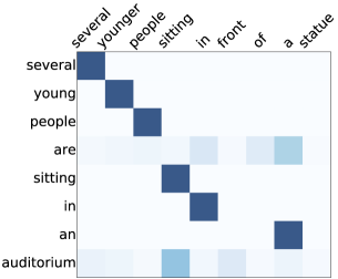
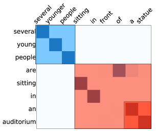
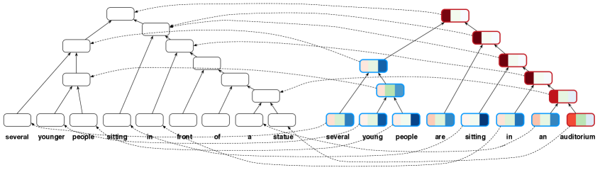
Our first example is shown in Figure 4 (a) and (b), with premise “several younger people sitting in front of a statue”, and hypothesis “several young people sitting in an auditorium”. Figure 4 (a) and (b) only show the word-level attention for brevity. In this example, note the hypothesis word “auditorium”, which has no explicit correspondence in the premise sentence, but indeed has an implicit correspondence “statue” that indicates the conflict relation. The standard attention model aligns “auditorium” to “sitting” since they more frequently co-occur, leading to an incorrect relation of “entailment” (not shown in Figure 5). The dual-attention model correctly finds the alignment between “auditorium” and “statue” since “sitting” is more likely to be aligned to the same word in the premise. The colored boxes in Figure 4 (b) show some important tree node alignment calculated by our model. The colors represent the entailment relation based on the alignment, as shown in Figure 5 (a).

In Figure 5 (a), each tree node is filled with three color stripes, whose darknesses show the confidences of the corresponding entailment relations. For this example, the contradiction relation from “statue” and “auditorium” flips every tree node from bottom up and finally make the final result contradiction, similar to our concept example in Figure 1.

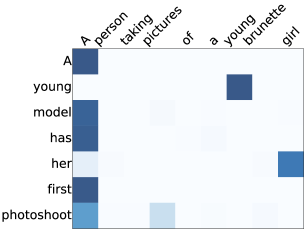
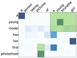
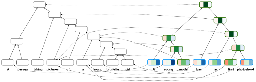
Another example with premise “a person taking pictures of a young brunette girl”, and hypothesis “a young model has her first photoshoot”. The word-level attentions are shown in Figure 4 (c) (d). The standard attention is uncertain about two words: 1) word “model” has several meanings, making it hard to find the right alignment, but in the perspective of from premise to hypothesis, it is easier since a girl is more likely to be a model. 2) Similar is for hypothesis word “photoshoot”, which can either be aligned to “a” or “pictures” but since “a” is aligned to other words, dual-attention aligns “photoshoot” to “pictures”.

In Figure 5 (b), we can see that there are two parts in the hypothesis indicates that the relation should be neutral: 1) “a young brunette girl” is not necessarily a “a young model”; and 2) the “pictures” taken are not necessarily “her first photoshoot”.

4.4 Discussion

Although many attention-based models, including our model, achieve superior results in the Stanford Natural Language Inference dataset, we still need to circumvent some problems to apply these neural models to more general textual entailment problems.

Despite those sentence pairs that require more common knowledge to find the entailment relations as we mentioned in Section 4.3, we are more interested in sentences that are difficult because they involve non-trivial linguistic properties.

Consider the following two pairs of sentences that are difficult for current attention and composition based models:

1. • Premise: The boy loves the girl.

   • Hypothesis: The girl loves the boy.

   Here the only difference between the two sentences is the order/structure of the words. To handle this problem the attention-based models should take the reordering into consideration when composing entailment relations.

2. • Premise: A stuffed animal on the couch.

   • Hypothesis: An animal on the couch.

   In this example, almost every hypothesis word occurs in the premise sentence, but it is difficult to infer that “a stuffed animal” is not “an animal”. While in most cases the monotonicity of entailment suggests that a word deletion in the premise sentence either leads to entailment, e.g., “a cute animal” entails “an animal”, or a reverse entailment, e.g., “some animal” reverse entails “animal” (See ?) for more details), but for words like “stuffed” it is quite different: their monotonicity directions depend on the nouns being modified, e.g., “a stuffed animal” does not entails “an animal”, but “a stuffed toy” entails “a toy”. This observation suggests that we might need to consider phrases like “stuffed animal” as a whole instead of treating the two words separately and then composing the entailment relations.

In addition, training of the neural models rely on large training corpora, which makes it difficult to directly apply neural models on traditional RTE datasets, e.g., the Pascal RTE dataset [Dagan et al., 2006] and the FraCaS dataset [Cooper et al., 1996], which are usually small and contain many named entities that are hard for neural models to identify.

5 Conclusion

We have presented an approach to model the composition of the entailment relation following the tree structure for the sentence entailment task. We adapted the attention model for tree structures. Experiments show that our model bring significant improvements in accuracy, and is easy to interpret.

References

- [Ba et al., 2015] Jimmy Ba, Ruslan R Salakhutdinov, Roger B Grosse, and Brendan J Frey. 2015. Learning wake-sleep recurrent attention models. In Advances in Neural Information Processing Systems, pages 2575–2583.
- [Bahdanau et al., 2014] Dzmitry Bahdanau, Kyunghyun Cho, and Yoshua Bengio. 2014. Neural machine translation by jointly learning to align and translate. arXiv preprint arXiv:1409.0473.
- [Bowman et al., 2015] Samuel R. Bowman, Gabor Angeli, Christopher Potts, and Christopher D. Manning. 2015. A large annotated corpus for learning natural language inference. In Proceedings of the 2015 Conference on Empirical Methods in Natural Language Processing, pages 632–642, Lisbon, Portugal, September. Association for Computational Linguistics.
- [Cheng et al., 2016] Jianpeng Cheng, Li Dong, and Mirella Lapata. 2016. Long short-term memory-networks for machine reading. arXiv preprint arXiv:1601.06733.
- [Cohn et al., 2016] Trevor Cohn, Cong Duy Vu Hoang, Ekaterina Vymolova, Kaisheng Yao, Chris Dyer, and Gholamreza Haffari. 2016. Incorporating structural alignment biases into an attentional neural translation model. arXiv preprint arXiv:1601.01085.
- [Cooper et al., 1996] Robin Cooper, Dick Crouch, Jan Van Eijck, Chris Fox, Johan Van Genabith, Jan Jaspars, Hans Kamp, David Milward, Manfred Pinkal, Massimo Poesio, et al. 1996. Using the framework. Technical report, Technical Report LRE 62-051 D-16, The FraCaS Consortium.
- [Dagan et al., 2006] Ido Dagan, Oren Glickman, and Bernardo Magnini. 2006. The pascal recognising textual entailment challenge. In Machine learning challenges. evaluating predictive uncertainty, visual object classification, and recognising tectual entailment, pages 177–190. Springer.
- [Filice et al., 2015] Simone Filice, Giovanni Da San Martino, and Alessandro Moschitti. 2015. Structural representations for learning relations between pairs of texts. In Proceedings of the 53rd Annual Meeting of the Association for Computational Linguistics, Beijing, China, July. Association for Computational Linguistics.
- [Hochreiter and Schmidhuber, 1997] Sepp Hochreiter and Jürgen Schmidhuber. 1997. Long short-term memory. Neural computation, 9(8):1735–1780.
- [Kingma and Ba, 2014] Diederik Kingma and Jimmy Ba. 2014. Adam: A method for stochastic optimization. arXiv preprint arXiv:1412.6980.
- [MacCartney and Manning, 2009] Bill MacCartney and Christopher D Manning. 2009. An extended model of natural logic. In Proceedings of the eighth international conference on computational semantics, pages 140–156. Association for Computational Linguistics.
- [Mnih et al., 2014] Volodymyr Mnih, Nicolas Heess, Alex Graves, et al. 2014. Recurrent models of visual attention. In Advances in Neural Information Processing Systems, pages 2204–2212.
- [Pennington et al., 2014] Jeffrey Pennington, Richard Socher, and Christopher D. Manning. 2014. Glove: Global vectors for word representation. In Proceedings of the 2014 Conference on Empirical Methods in Natural Language Processing (EMNLP 2014), pages 1532–1543.
- [Rocktäschel et al., 2015] Tim Rocktäschel, Edward Grefenstette, Karl Moritz Hermann, Tomáš Kočiskỳ, and Phil Blunsom. 2015. Reasoning about entailment with neural attention. arXiv preprint arXiv:1509.06664.
- [Socher et al., 2013] Richard Socher, Alex Perelygin, Jean Y Wu, Jason Chuang, Christopher D Manning, Andrew Y Ng, and Christopher Potts. 2013. Recursive deep models for semantic compositionality over a sentiment treebank. In Proceedings of the conference on empirical methods in natural language processing (EMNLP), volume 1631, page 1642. Citeseer.
- [Tai et al., 2015] Kai Sheng Tai, Richard Socher, and Christopher D. Manning. 2015. Improved semantic representations from tree-structured long short-term memory networks. In Proceedings of the 53rd Annual Meeting of the Association for Computational Linguistics and the 7th International Joint Conference on Natural Language Processing (Volume 1: Long Papers), pages 1556–1566, Beijing, China, July. Association for Computational Linguistics.
- [Tian et al., 2014] Ran Tian, Yusuke Miyao, and Takuya Matsuzaki. 2014. Logical inference on dependency-based compositional semantics. In Proceedings of ACL, pages 79–89.
- [Wang and Jiang, 2015] Shuohang Wang and Jing Jiang. 2015. Learning natural language inference with lstm. arXiv preprint arXiv:1512.08849.
- [Wang and Manning, 2010] Mengqiu Wang and Christopher D Manning. 2010. Probabilistic tree-edit models with structured latent variables for textual entailment and question answering. In Proceedings of the 23rd International Conference on Computational Linguistics, pages 1164–1172. Association for Computational Linguistics.
- [Watanabe et al., 2012] Yotaro Watanabe, Junta Mizuno, Eric Nichols, Naoaki Okazaki, and Kentaro Inui. 2012. A latent discriminative model for compositional entailment relation recognition using natural logic. In COLING, pages 2805–2820.
- [Xu et al., 2015] Kelvin Xu, Jimmy Ba, Ryan Kiros, Aaron Courville, Ruslan Salakhutdinov, Richard Zemel, and Yoshua Bengio. 2015. Show, attend and tell: Neural image caption generation with visual attention. arXiv preprint arXiv:1502.03044.
- [Zanzotto et al., 2009] Fabio Massimo Zanzotto, Marco Pennacchiotti, and Alessandro Moschitti. 2009. A machine learning approach to textual entailment recognition. Natural Language Engineering, 15(04):551–582.
- [Zaremba et al., 2014] Wojciech Zaremba, Ilya Sutskever, and Oriol Vinyals. 2014. Recurrent neural network regularization. arXiv preprint arXiv:1409.2329.