Reynolds-number dependence of the dimensionless dissipation rate in homogeneous magnetohydrodynamic turbulence

Abstract

This paper examines the behavior of the dimensionless dissipation rate $C_{\varepsilon}$ for stationary and nonstationary magnetohydrodynamic (MHD) turbulence in presence of external forces. By combining with previous studies for freely decaying MHD turbulence, we obtain here both the most general model equation for $C_{\varepsilon}$ applicable to homogeneous MHD turbulence and a comprehensive numerical study of the Reynolds number dependence of the dimensionless total energy dissipation rate at unity magnetic Prandtl number. We carry out a series of medium to high resolution direct numerical simulations of mechanically forced stationary MHD turbulence in order to verify the predictions of the model equation for the stationary case. Furthermore, questions of nonuniversality are discussed in terms of the effect of external forces as well as the level of cross- and magnetic helicity. The measured values of the asymptote $C_{\varepsilon,\infty}$ lie between $0.193\leqslant C_{\varepsilon,\infty}\leqslant 0.268$ for free decay, where the value depends on the initial level of cross- and magnetic helicities. In the stationary case we measure $C_{\varepsilon,\infty}=0.223$.

I Introduction

The dynamics of conducting fluids is relevant to many areas in geo- and astrophysics as well as in engineering and industrial applications. Often the flow is turbulent, and the interaction of the turbulent flow with the magnetic field leads to considerable complexity. Being a multi-parameter problem, techniques that have been successfully applied to turbulence in nonconducting fluids sometimes fail to deliver unambiguous predictions in magnetohydrodynamic (MHD) turbulence. This concerns e.g. the prediction of inertial range scaling exponents by extension of Kolmogorov’s arguments Kolmogorov (1941) to MHD, and considerable effort has been put into the further understanding of inertial range cascade(s) in MHD turbulence Iroshnikov (1964); Kraichnan (1965); Goldreich and Sridhar (1995); Boldyrev (2005, 2006); Beresnyak and Lazarian (2006); Mason et al. (2006); Gogoberidze (2007). The difficulties are partly due to the many different configurations that can arise in MHD turbulence because of e.g. anisotropy, different levels of vector field correlations, different values of the dissipation coefficients and different types of external forces, and as such are connected to the question of universality in MHD turbulence Dallas and Alexakis (2013a, b); Wan et al. (2012); Schekochihin et al. (2008); Mininni (2011); Grappin et al. (1983); A. Pouquet and P. Mininni and D. Montgomery and A. Alexakis (2008); Beresnyak (2011); Boldyrev et al. (2011); Grappin and Müller (2010); Lee et al. (2010); Servidio et al. (2008). The behavior of the (dimensionless) dissipation rate is representative of this problem, in the sense that the aforementioned properties of MHD turbulence influence the energy transfer across the scales, i.e. the cascade dynamics Frisch et al. (1975); Pouquet et al. (1976); Pouquet and Patterson (1978); Biskamp (1993); Dallas and Alexakis (2013b); Alexakis (2013), and thus the amount of energy that is eventually dissipated at the small scales.

The behavior of the total dissipation rate in a turbulent non-conducting fluid is a well-studied problem. As such it has been known for a long time that the total dissipation rate in both stationary and freely decaying homogeneous isotropic turbulence tends to a constant value with increasing Reynolds number following a well-known characteristic curve Sreenivasan (1984, 1998); McComb (2014); McComb et al. (2015a); Yeung et al. (2015); Jagannathan and Donzis (2016). For statistically steady isotropic turbulence this curve can be approximated by the real-space stationary energy balance equation, where the asymptote is connected to the maximal inertial flux of kinetic energy McComb et al. (2015a). The corresponding problem in MHD has received much less attention, however, recent numerical results for freely decaying MHD turbulence at unity magnetic Prandtl number report similar behavior. Mininni and Pouquet Mininni and Pouquet (2009) carried out direct numerical simulations (DNSs) of freely decaying homogeneous MHD turbulence without a mean magnetic field, showing that the temporal maximum of the total dissipation rate $\varepsilon(t)$ became independent of Reynolds number at a Taylor-scale Reynolds number $R_{\lambda}$ (measured at the peak of $\varepsilon(t)$) of about 200. Dallas and Alexakis Dallas and Alexakis (2014) measured the dimensionless dissipation rate $C_{\varepsilon}$ also from DNS data for free decay for random initial fields with strong correlations between the velocity field and the current density. Again, it was found that $C_{\varepsilon}\to const.$ with increasing Reynolds number. Interestingly, a comparison with the data of Ref. Mininni and Pouquet (2009) showed that the approach to the asymptote was slower than for the data of Ref. Mininni and Pouquet (2009), suggesting an influence of the level of certain vector field correlations on the approach to the asymptote. A theoretical model for dissipation rate scaling in freely decaying MHD turbulence was put forward recently Linkmann et al. (2015) based on the von Kármán-Howarth energy balance equations (vKHE) in terms of Elsässer fields Politano and Pouquet (1998). For unity magnetic Prandtl number it predicts the dependence of $C_{\varepsilon}$ on a generalized Reynolds number $R_{-}\equiv z^{-}L^{+}/(\nu+\mu)$, with $z^{-}$ denoting the root-mean-square value of one Elsässer field, $L^{+}$ the integral scale corresponding to the other Elsässer field, while $\nu$ and $\mu$ are the kinematic viscosity and the magnetic resistivity, respectively. The model equation has the following form

$$C_{\varepsilon}=C_{\varepsilon,\infty}+\frac{C}{R_{-}}+\frac{D}{R_{-}^{2}}+O(R_{-}^{-3})\ ,$$ (1)

where $C$ and $D$ are time-dependent coefficients depending on several parameters, which themselves depend on the magnetic, cross- and kinetic helicities. The predictions of this equation were subsequently tested against data obtained from medium to high resolution DNSs of freely decaying homogeneous MHD turbulence leading to a very good agreement between theory and data.

In summary, there is compelling numerical and theoretical evidence for finite dissipation in freely decaying MHD turbulence at least for unity magnetic Prandtl number $Pm=\nu/\mu$, while so far no systematic results for the stationary case have been reported. In this paper we extend the derivation carried out in Ref. Linkmann et al. (2015) to include the effects of external forces and we present the first systematic study of dissipation rate scaling for stationary MHD turbulence. In order to be able to test the model equation against DNS data for a large range of generalized Reynolds numbers, we concentrate on the case $Pm=1$. The most general form of Eq. (1) for nonstationary flows with large-scale external forcing is derived, which can be applied to freely decaying and stationary flows by setting the corresponding terms to zero. This generalization of Eq. (1) is the first main result of the paper, it is applicable to both freely decaying and stationary MHD turbulence. It implies that the dissipation rate of total energy is finite in the limit $R_{-}\to\infty$ in analogy to hydrodynamics, and highlights the dependence of the coefficients $C$ and $D$ on the external forces. As such, Eq. (1) predicts nonuniversal values of the asymptotic value $C_{\varepsilon,\infty}$ of the dimensionless dissipation rate in the infinite Reynolds number limit and of the approach to the asymptote for a variety of MHD flows. The resulting theoretical predictions for the stationary case are compared to DNS data for stationary MHD turbulence for three different types of mechanical forcing while the results for the freely decaying case Linkmann et al. (2015) are reviewed for completeness. The DNS data shows good agreement with Eq. (1) and the different forcing schemes have no measurable effect on the values of the coefficients in Eq. (1). The measured values of $C_{\varepsilon,\infty}$ lie between $0.193\leqslant C_{\varepsilon,\infty}\leqslant 0.268$ for free decay, where the value depends on the initial level of cross- and magnetic helicities. In the stationary case we measure $C_{\varepsilon,\infty}=0.223$.

This paper is organized as follows. We begin by reviewing the formulation of the MHD equations in terms of Elsässer fields in Sec. II where we introduce the basic quantities we aim to study in both formulations of the MHD equations. In Section III we extend the derivation put forward in Ref. Linkmann et al. (2015) to nonstationary MHD turbulence. The model equation is verified against DNS data for statistically steady MHD turbulence and the comparison to data for freely decaying MHD turbulence presented in Ref. Linkmann et al. (2015) is reviewed in Sec. IV, where special emphasis is given to the question of nonuniversality of MHD turbulence in the context of external forces and the level of cross- and magnetic helicities. Our results are summarized and discussed in the context of related work in hydrodynamic and MHD turbulence in Sec. V, where we also outline suggestions for further work.

II The total dissipation in terms of Elsässer fields

In this paper we consider statistically homogeneous MHD turbulence in the absence of a background magnetic field. The flow is taken to be incompressible, leading to the following set of coupled partial differential equations

$$\partial_{t}\bm{u} =-\frac{1}{\rho}\nabla P-(\bm{u}\cdot\nabla)\bm{u}+\frac{1}{\rho}(\nabla\times\bm{b})\times\bm{b}+\nu\Delta\bm{u}+\bm{f}_{u}\ ,$$ (2)

$$\partial_{t}\bm{b} =(\bm{b}\cdot\nabla)\bm{u}-(\bm{u}\cdot\nabla)\bm{b}+\mu\Delta\bm{b}+\bm{f}_{b}\ ,$$ (3)

$$\nabla\cdot\bm{u}=0\ \ \mbox{and}\ \ \nabla\cdot\bm{b}=0\ ,$$ (4)

where $\bm{u}$ denotes the velocity field, $\bm{b}$ the magnetic induction expressed in Alfvén units, $\nu$ the kinematic viscosity, $\mu$ the magnetic resistivity, $P$ the thermodynamic pressure, $\bm{f}_{u}$ and $\bm{f}_{b}$ are external mechanical and electromagnetic forces, which may be present, and $\rho$ denotes the density which is set to unity for convenience. Equations (2)-(4) are considered on a three-dimensional domain $\Omega$, which due to homogeneity can either be the full space $\mathbb{R}^{3}$ or a subdomain $[0,L_{box})^{3}$ with periodic boundary conditions. The MHD equations (2)-(4) can be formulated more symmetrically using Elsässer variables $\bm{z^{\pm}}=\bm{u}\pm\bm{b}$ Elsässer (1950)

$$\partial_{t}\bm{z}^{\pm} =-\frac{1}{\rho}\nabla\tilde{P}-(\bm{z}^{\mp}\cdot\nabla)\bm{z}^{\pm}+(\nu+\mu)\Delta\bm{z}^{\pm}+(\nu-\mu)\Delta\bm{z}^{\mp}+\bm{f}^{\pm}\ ,$$ (5)

$$\nabla\cdot\bm{z}^{\pm}=0\ ,$$ (6)

where $\bm{f}^{\pm}=\bm{f}_{u}\pm\bm{f}_{b}$ and the pressure $\tilde{P}$ consists of the sum of the thermodynamic pressure $P$ and the magnetic pressure $\rho|\bm{b}|^{2}/2$. Which formulation of the MHD equations is chosen often depends on the physical problem, for some problems the Elsässer formalism is technically convenient, while the formulation using the primary fields $\bm{u}$ and $\bm{b}$ facilitates physical understanding. The ideal invariants total energy $E(t)$, cross-helicity $H_{c}(t)$ and magnetic helicity $H_{m}(t)$ are given in the respective formulations of the MHD equation by

$$E(t) =\frac{1}{2}\int_{\Omega}d\bm{k}\ \langle|\hat{\bm{u}}(\bm{k},t)|^{2}+|\hat{\bm{b}}(\bm{k},t)|^{2}\rangle=\frac{1}{4}\int_{\Omega}d\bm{k}\ \langle|\hat{\bm{z}}^{+}(\bm{k},t)|^{2}+|\hat{\bm{z}}^{-}(\bm{k},t)|^{2}\rangle\ ,$$ (7)

$$H_{c}(t) =\int_{\Omega}d\bm{k}\ \langle\hat{\bm{u}}(\bm{k},t)\cdot\hat{\bm{b}}(-\bm{k},t)\rangle=\frac{1}{4}\int_{\Omega}d\bm{k}\ \langle|\hat{\bm{z}}^{+}(\bm{k},t)|^{2}-|\hat{\bm{z}}^{-}(\bm{k},t)|^{2}\rangle\ ,$$ (8)

$$H_{m}(t) =\int_{\Omega}d\bm{k}\ \langle\hat{\bm{a}}(\bm{k},t)\cdot\hat{\bm{b}}(-\bm{k},t)\rangle=\frac{1}{4}\int_{\Omega}d\bm{k}\ \left\langle\left[\frac{i\bm{k}}{k^{2}}\times(\hat{\bm{z}}^{+}(\bm{k},t)-\hat{\bm{z}}^{-}(\bm{k},t))\right]\cdot(\hat{\bm{z}}^{+}(-\bm{k},t)-\hat{\bm{z}}^{-}(-\bm{k},t))\right\rangle\ ,$$ (9)

with $\hat{\bm{b}}$, $\hat{\bm{u}}$ and $\hat{\bm{z}}^{\pm}$ denoting the respective Fourier transforms of the magnetic, velocity and Elsässer fields, while $\hat{\bm{a}}$ is the Fourier transform of the magnetic vector potential $\bm{a}$. The angled brackets indicate an ensemble average. Equation (9) is gauge-independent as shown in Appendix A.

We now motivate the use of the Elsässer formulation for the study of the dimensionless dissipation coefficient in MHD. In hydrodynamics, the dimensionless dissipation coefficient $C_{\varepsilon,u}$ is defined in terms of the Taylor surrogate expression for the total dissipation rate, $U^{3}/L_{u}$, where $U$ denotes the root-mean-square (rms) value of the velocity field and $L_{u}$ the integral scale defined with respect to the velocity field, as

$$C_{\varepsilon,u}\equiv\varepsilon_{kin}\frac{L_{u}}{U^{3}}\ .$$ (10)

However, in MHD there are several quantities that may be used to define an MHD analogue to the Taylor surrogate expression, such as the rms value $B$ of the magnetic field, one of the different length scales defined with respect to either $\bm{b}$ or $\bm{u}$, or the total energy.

Since the total dissipation in MHD turbulence should be related to the flux of total energy through different scales, one may think of defining a dimensionless dissipation coefficient for MHD in terms of the total energy. However, this would lead to a nondimensionalization of the hydrodynamic transfer term $\bm{u}\cdot(\bm{u}\cdot\nabla)\bm{u}$ with a magnetic quantity. This can be seen by considering the analog of the von Kármán-Howarth energy balance equation in real space Chandrasekhar (1951) stated here for the case of free decay

$$-d_{t}E(t)=\varepsilon(t)= -\partial_{t}(B_{LL}^{uu}(r,t)+B_{LL}^{bb}(r,t))+\frac{3}{2r^{4}}\partial_{r}\left(\frac{r^{4}}{6}B_{LLL}^{uuu}(r,t)+r^{4}C_{LLL}^{bbu}(r,t)\right)$$

$$\ \ \ +\frac{6}{r}C^{bub}(r,t)+\frac{1}{r^{4}}\partial_{r}\left(r^{4}\partial_{r}(\nu B_{LL}^{uu}(r,t)+\mu B_{LL}^{bb}(r,t))\right)\ ,$$ (11)

where $B_{LL}^{uu}$, $B_{LL}^{bb}$ and $B_{LLL}^{uuu}$ are the longitudinal structure functions, $C_{LLL}^{bbu}$ the longitudinal correlation function and $C^{bub}$ another correlation function. The longitudinal structure and correlation functions are given by

$$B_{LL}^{uu}(r,t) =\langle(\delta u_{L}(\bm{r},t))^{2}\rangle\ ,$$ (12)

$$B_{LL}^{bb}(r,t) =\langle(\delta b_{L}(\bm{r},t))^{2}\rangle\ ,$$ (13)

$$B_{LLL}^{uuu}(r,t) =\langle(\delta u_{L}(\bm{r},t))^{3}\rangle\ ,$$ (14)

$$C_{LLL}^{bbu}(r,t) =\langle u_{L}(\bm{x},t)b_{L}(\bm{x},t)b_{L}(\bm{x}+\bm{r},t)\rangle\ ,$$ (15)

where $r=|\bm{r}|$ and $v_{L}=\bm{v}\cdot\bm{r}/r$ denotes the longitudinal component of a vector field $\bm{v}$, that is its component parallel to the displacement vector $\bm{r}$, and

$$\delta v_{L}(\bm{r})=[\bm{v}(\bm{x}+\bm{r})-\bm{v}(\bm{x})]\cdot\frac{\bm{r}}{r}\ ,$$ (16)

its longitudinal increment. The function $C^{bub}$ is defined through the third-order correlation tensor

$$C_{ij,k}^{bub}(\bm{r},t) =\langle(u_{i}(\bm{x})b_{j}(\bm{x})-b_{i}(\bm{x})u_{j}(\bm{x}))b_{k}(\bm{x}+\bm{r})\rangle=C^{bub}(r,t)\left(\frac{r_{j}}{r}\delta_{ik}-\frac{r_{i}}{r}\delta_{jk}\right).\$$ (17)

As can be seen from their respective definitions, the functions $C_{LLL}^{bbu}$ and $C^{bub}$ scale with $B^{2}U$ while the function $B_{LLL}^{uuu}$ scales with $U^{3}$. If Eq. (11) were to be nondimensionalized with respect to the total energy then the purely hydrodynamic term $B_{LLL}^{uuu}$ would be scaled partially by a magnetic quantity.

This problem of inconsistent nondimensionalization can be avoided by working with Elsässer fields, which requires an expression for the total dissipation rate $\varepsilon(t)$ in terms of Elsässer fields. The total rate of energy dissipation in MHD turbulence is given by the sum of Ohmic and viscous dissipation

$$\varepsilon(t)=\varepsilon_{mag}(t)+\varepsilon_{kin}(t)\ ,$$ (18)

where

$$\varepsilon_{mag}(t) =\mu\int_{\Omega}d\bm{k}\ k^{2}\langle|\hat{\bm{b}}(\bm{k},t)|^{2}\rangle\ ,$$ (19)

$$\varepsilon_{kin}(t) =\nu\int_{\Omega}d\bm{k}\ k^{2}\langle|\hat{\bm{u}}(\bm{k},t)|^{2}\rangle\ .$$ (20)

Similarly, the total dissipation rate can be decomposed into its respective contributions from the Elsässer dissipation rates

$$\varepsilon(t)=\frac{1}{2}\big{(}\varepsilon_{+}(t)+\varepsilon_{-}(t)\big{)}\ ,$$ (21)

where the Elsässer dissipation rates are defined as

$$\varepsilon^{\pm}(t)=\nu_{+}\int_{\Omega}d\bm{k}\ k^{2}\langle|\hat{\bm{z}}^{\pm}(\bm{k},t)|^{2}\rangle+\nu_{-}\int_{\Omega}d\bm{k}\ k^{2}\langle\hat{\bm{z}}^{\pm}(\bm{k},t)\cdot\hat{\bm{z}}^{\mp}(-\bm{k},t)\rangle\ ,$$ (22)

with $\nu_{\pm}=(\nu\pm\mu)$. The total dissipation rate relates to the sum of the Elsässer dissipation rates

$$\varepsilon^{+}(t)+\varepsilon^{-}(t)=\varepsilon(t)+\varepsilon_{H_{c}}(t)+\varepsilon(t)-\varepsilon_{H_{c}}(t)=2\varepsilon(t)\ ,$$ (23)

where the cross-helicity dissipation rate $\varepsilon_{H_{c}}$ is given by

$$\varepsilon_{H_{c}}(t)=\frac{1}{2}\big{(}\varepsilon^{+}(t)-\varepsilon^{-}(t)\big{)}\ .$$ (24)

Since this paper is concerned with both stationary and nonstationary flows, the total energy input rate $\iota$ must also be considered. Similar to the dissipation rate, the input rate can be split up into either kinetic and magnetic contributions or the Elsässer contributions $\iota^{\pm}(t)$

$$\iota(t) =\iota_{mag}(t)+\iota_{kin}(t)$$ (25)

$$\iota(t) =\frac{1}{2}\big{(}\iota^{+}(t)+\iota^{-}(t)\big{)}\ .$$ (26)

The latter equation can be rewritten as

$$\iota^{+}(t)=\iota(t)+\frac{1}{2}\left(\iota^{+}(t)-\iota^{-}(t)\right)=\iota(t)+\iota_{H_{c}}(t)\ ,$$ (27)

where $\iota_{H_{c}}$ denotes the input rate of the cross-helicity.

III Derivation of the equation

Since the total dissipation rate can be expressed either in terms of the Elsässer fields or the primary fields $\bm{u}$ and $\bm{b}$, it should be possible to describe it also by the vKHE for $\bm{z}^{\pm}$ Politano and Pouquet (1998). For the freely decaying case no further complication arises as the rate of change of total energy, which figures on the left-hand side of the energy balance, equals the total dissipation rate. However, in the more general case the rate of change of the total energy is given by the difference of energy input and dissipation. That is, in the most general case the total energy dissipation rate is given by

$$\varepsilon(t)=\iota(t)-d_{t}E(t)\ .$$ (28)

For the stationary case $d_{t}E(t)=0$ and one obtains $\varepsilon(t)=\iota(t)$. For the freely decaying case $\iota(t)=0$ and the change in total energy is due to dissipation only, that is $-d_{t}E(t)=\varepsilon(t)$. In terms of Elsässer variables $\varepsilon(t)$ can also be expressed as

$$\varepsilon(t)=\iota(t)-d_{t}E(t)=\iota(t)-d_{t}E^{\pm}(t)\mp d_{t}H_{c}(t)\ ,$$ (29)

where $E^{\pm}(t)$ denote the Elsässer energies. Since we have related the total dissipation rate to the rate of change of the Elsässer energies, we are now in a position to consider the energy balance equations for $\bm{z}^{\pm}$, which are stated here for the most general case of homogeneous forced nonstationary MHD flows without a mean magnetic field

$$-\partial_{t}E^{\pm}(t)+I^{\pm}(r,t)= -\frac{3}{4}\partial_{t}B_{LL}^{\pm\pm}(r,t)-\frac{\partial_{r}}{r^{4}}\left(\frac{3r^{4}}{2}C^{\pm\mp\pm}_{LL,L}(r,t)\right)$$

$$\ \ \ +\frac{3}{4r^{4}}\partial_{r}\left(r^{4}\partial_{r}(\nu+\mu)B^{\pm}_{LL}(r,t)\right)$$

$$\ \ \ +\frac{3}{4r^{4}}\partial_{r}\left(r^{4}\partial_{r}(\nu-\mu)B^{\mp}_{LL}(r,t)\right)\ ,$$ (30)

where $I^{\pm}(r,t)$ are (scale-dependent) energy input terms and

$$C^{\pm\mp\mp}_{LL,L}(r,t) =\langle z_{L}^{\pm}(\bm{x},t)z_{L}^{\mp}(\bm{x},t)z_{L}^{\pm}(\bm{x}+\bm{r},t)\rangle\ ,$$ (31)

$$B_{LL}^{\pm\pm}(r,t) =\langle(\delta z_{L}^{\pm}(\bm{r},t))^{2}\rangle\ ,$$ (32)

$$B_{LL}^{\pm\mp}(r,t) =\langle\delta z_{L}^{\pm}(\bm{r},t)\delta z_{L}^{\mp}(\bm{r},t)\rangle\ ,$$ (33)

are the third-order longitudinal correlation function and the second-order structure functions of the Elsässer fields, respectively. As can be seen from the definition, the third-order correlation function scales with $(z^{\pm})^{2}z^{\mp}$, where $z^{\pm}$ denote the respective rms values of the Elsässer fields. This permits a consistent nondimensionalization of the Elsässer vKHE using the appropriate quantities defined in terms of Elsässer variables. As such the complication that arose if the energy balance was written in terms of $\bm{b}$ and $\bm{u}$ can be circumvented. This motivates the definition of the dimensionless Elsässer dissipation rates as

$$C_{\varepsilon}^{\pm}(t)\equiv\frac{\varepsilon(t)L_{\pm}(t)}{z^{\pm}(t)^{2}z^{\mp}(t)}\ ,$$ (34)

where

$$L_{\pm}(t)=\frac{3\pi}{8E^{\pm}(t)}\int_{\Omega}d\bm{k}\ k^{-1}\langle|\bm{z}^{\pm}(\bm{k},t)|^{2}\rangle\ ,$$ (35)

are the integral scales defined with respect to $\bm{z}^{\pm}$ . For balanced MHD turbulence, i.e. $H_{c}=0$, one should expect $C_{\varepsilon}^{+}(t)=C_{\varepsilon}^{-}(t)$, since

$$E^{\pm}(t)=2E(t)\pm 2H_{c}(t)=2E(t)\ .$$ (36)

Therefore all quantities defined with respect to the rms fields $z^{+}$ and $z^{-}$ should be the same in this case. Finally, the dimensionless dissipation rate $C_{\varepsilon}(t)$ is defined as

$$C_{\varepsilon}(t)=C_{\varepsilon}^{+}(t)+C_{\varepsilon}^{-}(t)\equiv\frac{\varepsilon(t)L_{+}(t)}{{z^{+}(t)}^{2}z^{-}(t)}+\frac{\varepsilon(t)L_{-}(t)}{{z^{-}(t)}^{2}z^{+}(t)}\ .$$ (37)

Using the definition given in Eq. (34), the Elsässer energy balance equations (30) can now be consistently nondimensionalized. For conciseness the explicit time and spatial dependences are from now on omitted, unless there is a particular point to make.

III.1 Dimensionless von Kármán-Howarth equations

By introducing the nondimensional variables $\sigma_{\pm}=r/L_{\pm}$ Wan et al. (2012) and non-dimensionalising Eq. (30) as proposed in the definitions of $C_{\varepsilon}^{\pm}$ given in Eq. (34) one obtains

$$-\left(d_{t}E^{\pm}-I^{\pm}\right)\frac{L_{\pm}}{{z^{\pm}}^{2}z^{\mp}}= -\frac{1}{\sigma_{\pm}^{4}}\partial_{\sigma_{\pm}}\left(\frac{3\sigma_{\pm}^{4}C^{\pm\mp\pm}_{LL,L}}{2{z^{\pm}}^{2}z^{\mp}}\right)-\frac{L_{z^{\pm}}}{{z^{\pm}}^{2}z^{\mp}}\partial_{t}\frac{3B_{LL}^{\pm\pm}}{4}$$

$$+\frac{\mu+\nu}{L_{\pm}z^{\mp}}\frac{3}{4\sigma_{\pm}^{4}}\left(\sigma_{\pm}^{4}\partial_{\sigma_{\pm}}\frac{B_{LL}^{\pm\pm}}{{z^{\pm}}^{2}}\right)$$

$$+\frac{\nu-\mu}{L_{\pm}z^{\pm}}\frac{3}{4\sigma_{\pm}^{4}}\left(\sigma_{\pm}^{4}\partial_{\sigma_{\pm}}\frac{B_{LL}^{\pm\mp}}{{z^{\pm}}z^{\mp}}\right)\ .$$ (38)

Before proceeding further, the scale-dependent forcing term on the left-hand side of this equation needs to be analyzed in some detail in order to clarify its relation to the energy input rates $\iota$ and $\iota^{\pm}$. The Elsässer energy input $I^{\pm}$ is given by

$$I^{\pm}(r)=\frac{3}{r^{3}}\int_{0}^{r}dr^{\prime}r^{\prime 2}\langle\bm{z}^{\pm}(\bm{x}+\bm{r}^{\prime})\cdot\bm{f}^{\pm}(\bm{x})\rangle\ .$$ (39)

Since the energy input rate is given by $\iota^{\pm}=\langle\bm{z}^{\pm}(\bm{x})\cdot\bm{f}^{\pm}(\bm{x})\rangle$, the correlation function can be expressed as

$$\langle\bm{z}^{\pm}(\bm{x}+\bm{r})\cdot\bm{f}^{\pm}(\bm{x})\rangle=\iota^{\pm}\phi^{\pm}(r/L_{f})\ ,$$ (40)

where $\phi^{\pm}$ are dimensionless even functions of $r/L_{f}$ satisfying $\phi^{\pm}(0)=1$ and $L_{f}$ the characteristic scale of the forcing. At scales much smaller than the forcing scale, i.e. for $r/L_{f}<<1$, for suitable types of forces $\phi^{\pm}(r/L_{f})$ can be expanded in a Taylor series Novikov (1965), leading to the following expression for the energy input

$$I^{\pm}(r)=\frac{3}{r^{3}}\int_{0}^{r}dr^{\prime}r^{\prime 2}\iota^{\pm}\left[1+\left(\frac{r}{L_{f}}\right)^{2}\frac{\partial^{2}\phi^{\pm}}{2\partial(r/L_{f})^{2}}\Big{|}_{r/L_{f}=0}+O\left(\left(\frac{r}{L_{f}}\right)^{4}\right)\right]\ .$$ (41)

In the limit of infinite Reynolds number the inertial range extends through all wavenumbers, formally implying that $L_{f}\to\infty$, where Eq. (41) implies $I^{\pm}(r)\to\iota^{\pm}$. Therefore it should be possible to split the term $I^{\pm}(r)$ into a constant, $\iota^{\pm}$, and a scale-dependent term $J^{\pm}(r)$, which encodes the additional scale dependence introduced by realistic, finite Reynolds number forcing. For consistency, this scale-dependent term must vanish in the formal limit $Re\to\infty$. This can be achieved by writing $I^{\pm}(r)$ in terms of the correlation of the force and Elsässer field increments

$$I^{\pm}(r)=\iota^{\pm}-\frac{3}{2r^{3}}\int_{0}^{r}dr^{\prime}r^{\prime 2}\langle\delta\bm{z}^{\pm}\cdot\delta\bm{f}^{\pm}\rangle\ .$$ (42)

Therefore we define

$$J^{\pm}(r)=-\frac{3}{2r^{3}}\int_{0}^{r}dr^{\prime}r^{\prime 2}\langle\delta\bm{z}^{\pm}\cdot\delta\bm{f}^{\pm}\rangle\ ,$$ (43)

where $\lim_{Re\to\infty}J^{\pm}(r)=0$. Hence the energy input $I^{\pm}(r)$ can be expressed as the sum of the scale-independent energy input rate $\iota^{\pm}$ and a scale-dependent term which vanishes in the formal limit $Re\to\infty$

$$I^{\pm}(r)=\iota^{\pm}+J^{\pm}(r)\ ,$$ (44)

with $\lim_{Re\to\infty}J^{\pm}(r)=0$. Substitution of Eq. (44) into the nondimensionalized energy balance Eq. (III.1) leads to the dimensionless version of the Elsässer vKHE for homogeneous MHD turbulence in the most general case for nonstationary flows at any magnetic Prandtl number

$$C_{\varepsilon}^{\pm}= -\frac{\partial_{\sigma_{\pm}}}{\sigma_{\pm}^{4}}\left(\frac{3\sigma_{\pm}^{4}C^{\pm\mp\pm}_{LL,L}}{2{z^{\pm}}^{2}z^{\mp}}\right)+\frac{L_{\pm}}{{z^{\pm}}^{2}z^{\mp}}\left(\pm d_{t}H_{c}-\partial_{t}\frac{3B_{LL}^{\pm\pm}}{4}-J^{\pm}\mp\iota_{H_{c}}\right)$$

$$+\frac{1}{R_{\mp}}\frac{3\partial_{\sigma_{\pm}}}{2\sigma_{\pm}^{4}}\left(\sigma_{\pm}^{4}\partial_{\sigma_{\pm}}\frac{B_{LL}^{\pm\pm}}{{z^{\pm}}^{2}}\right)+\frac{1}{R^{\prime}_{\pm}}\frac{3\partial_{\sigma_{\pm}}}{2\sigma_{\pm}^{4}}\left(\sigma_{\pm}^{4}\partial_{\sigma_{\pm}}\frac{B_{LL}^{\pm\mp}}{{z^{\pm}}z^{\mp}}\right)\ ,$$ (45)

where $R_{\mp}$ and $R^{\prime}_{\pm}$ denote generalized large-scale Reynolds numbers given by

$$R_{\mp} =z^{\mp}L_{\pm}/(\nu+\mu)\ \ \mbox{and}\ \ R^{\prime}_{\pm}=z^{\pm}L_{\pm}/(\nu-\mu)\ .$$ (46)

In order to express Eq. (45) more concisely, the following dimensionless functions are defined

$$g^{\pm\mp\pm} =\frac{C^{\pm\mp\pm}_{LL,L}}{{z^{\pm}}^{2}z^{\mp}}\ ,$$ (47)

$$h^{\pm\pm} =\frac{B_{LL}^{\pm\pm}}{{z^{\pm}}^{2}}\ ,$$ (48)

$$h^{\pm\mp} =\frac{B_{LL}^{\pm\mp}}{{z^{\pm}}z^{\mp}}\ ,$$ (49)

$$H^{\pm\pm} =\frac{L_{\pm}}{{z^{\pm}}^{2}z^{\mp}}\partial_{t}B_{LL}^{\pm\pm}\ ,$$ (50)

$$F^{\pm} =\frac{L_{\pm}}{{z^{\pm}}^{2}z^{\mp}}J^{\pm}\ ,$$ (51)

$$G^{\pm} =\frac{L_{\pm}}{{z^{\pm}}^{2}z^{\mp}}d_{t}H_{c}\ ,$$ (52)

$$Q^{\pm} =\frac{L_{\pm}}{{z^{\pm}}^{2}z^{\mp}}\iota_{H_{c}}\ ,$$ (53)

such that Eq. (45) can be written as

$$C_{\varepsilon}^{\pm}= -\frac{\partial_{\sigma_{\pm}}}{\sigma_{\pm}^{4}}\left(\frac{3\sigma_{\pm}^{4}}{2}g^{\pm\mp\pm}\right)\pm G^{\pm}-\frac{3}{4}H^{\pm\pm}-F^{\pm}\mp Q^{\pm}$$

$$+\frac{3}{R_{\mp}}\frac{\partial_{\sigma_{\pm}}}{\sigma_{\pm}^{4}}\left(\sigma_{\pm}^{4}\partial_{\sigma_{\pm}}h^{\pm\pm}\right)+\frac{3}{R^{\prime}_{\mp}}\frac{\partial_{\sigma_{\pm}}}{\sigma_{\pm}^{4}}\left(\sigma_{\pm}^{4}\partial_{\sigma_{\pm}}h^{\pm\mp}\right)\ .$$ (54)

This equation can be applied to the two simpler cases of freely decaying and stationary MHD turbulence by setting the corresponding terms to zero. For the case of free decay there are no external forces therefore $F^{\pm}=0$, while for the stationary case the terms $G^{\pm}$ and $H^{\pm}$ vanish. A further simplification concerns the case $Pm=1$, that is $\nu=\mu$, where the inverse of the generalized Reynolds numbers $R^{\prime}_{\pm}$ vanish. In this case the evolution of $C_{\varepsilon}^{\pm}$ depends only on $R_{\mp}$, and an approximate analysis using asymptotic series is possible. Most numerical results are concerned with this case due to computational constraints, hence it would be very difficult to test an approximate equation against DNS data if not only $Re$ but also $Pm$ needs to be varied. From now on the magnetic Prandtl number is therefore set to unity, keeping in mind that the analysis could be extended to $Pm\neq 1$ provided the approximate equation derived in the following section is consistent with DNS data.

III.2 Asymptotic analysis for the case $Pm=1$

Equation (54) suggests a dependence of $C_{\varepsilon}^{\pm}$ on $1/R_{\mp}$, however, the structure and correlation functions also have a dependence on Reynolds number, which describes their deviation from their respective inertial-range forms. The highest derivative in Eq. (54) is multiplied by the small parameter $1/R_{\mp}$, which suggests that this equation may be viewed as singular perturbation problem amenable to asymptotic analysis Lundgren (2002). The Elsässer vKHE was rescaled by the rms values of the Elsässer fields and the corresponding integral length scales, where the integral scales are by definition the large-scale quantities, the interpretation in hydrodynamics usually being that they represent the size of the largest eddies. As such, the nondimensionalization was carried out with respect to quantities describing the large scales, that is, with respect to ‘outer’ variables. Hence outer asymptotic expansions of the nondimensional structure and correlation functions are considered with respect to the inverse of the (large-scale) generalized Reynolds numbers $1/R_{\mp}$. We point out that the case $Pm\neq 1$ would require expansions in two parameters, where the cases $Pm>1$ and $Pm<1$ must be treated separately due to a sign change in $R^{\prime}_{\pm}$ between the two cases.

The formal asymptotic series of a generic function $f$ [used for conciseness in place of the functions on the right-hand side of Eq. (54)] up to second order in $1/R_{\mp}$ reads

$$f=f_{0}+\frac{1}{R_{\mp}}f_{1}+\frac{1}{R_{\mp}^{2}}f_{2}+O(R_{\mp}^{-3})\ .$$ (55)

After substitution of the expansions into Eq. (54), collecting terms of the same order in $1/R_{\mp}$, one arrives at equations describing the behavior of $C_{\varepsilon}^{+}$ and $C_{\varepsilon}^{-}$

$$C_{\varepsilon}^{\pm}=C_{\varepsilon,\infty}^{\pm}+\frac{C^{\pm}}{R_{\mp}}+\frac{D^{\pm}}{R_{\mp}^{2}}+O(R_{\mp}^{-3})\ ,$$ (56)

up to second order in $1/R_{\mp}$, using the coefficients $C_{\varepsilon,\infty}^{\pm}$, $C^{\pm}$ and $D^{\pm}$ defined as

$$C_{\varepsilon,\infty}^{\pm} =-\frac{\partial_{\sigma_{\pm}}}{\sigma_{\pm}^{4}}\left(\frac{3\sigma_{\pm}^{4}}{2}g_{0}^{\pm\mp\pm}\right)\pm G^{\pm}-\frac{3}{4}H_{0}^{\pm\pm}\mp Q^{\pm}\ ,$$ (57)

$$C^{\pm} =\frac{3\partial_{\sigma_{\pm}}}{\sigma_{\pm}^{4}}\left[\sigma_{\pm}^{4}\left(\partial_{\sigma_{\pm}}h_{0}^{\pm\pm}-\frac{g_{1}^{\pm\mp\pm}}{2}\right)\right]\mp F_{1}^{\pm}-\frac{3}{4}H_{1}^{\pm\pm}\ ,$$ (58)

$$D^{\pm} =\frac{3\partial_{\sigma_{\pm}}}{\sigma_{\pm}^{4}}\left[\sigma_{\pm}^{4}\left(\partial_{\sigma_{\pm}}h_{1}^{\pm\pm}-\frac{g_{2}^{\pm\mp\pm}}{2}\right)\right]\mp F_{2}^{\pm}-\frac{3}{4}H_{2}^{\pm\pm}\ ,$$ (59)

in order to write Eq. (54) in a more concise way. The zero-order term in the expansion of the function $F^{\pm}$ vanishes, since $F^{\pm}$ corresponds to the scale-dependent part $J^{\pm}$ of the energy input which vanishes in the limit $R_{\mp}\to\infty$, hence $F_{0}^{\pm}=0$. According to the definition of $C_{\varepsilon}$ in Eq. (37), the asymptote $C_{\varepsilon,\infty}$ is given by

$$C_{\varepsilon,\infty}=C_{\varepsilon,\infty}^{+}+C_{\varepsilon,\infty}^{-}\ ,$$ (60)

and using the definition of the generalized Reynolds numbers, which implies $R_{+}=(L_{-}/L_{+})(z^{+}/z^{-})R_{-}$ one can define

$$C=C^{+}+\frac{L_{-}}{L_{+}}\frac{z^{+}}{z^{-}}C^{-}\ ,$$ (61)

($D$ is defined analogously), resulting in the following expression for the dimensionless dissipation rate

$$C_{\varepsilon}=C_{\varepsilon,\infty}+\frac{C}{R_{-}}+\frac{D}{R_{-}^{2}}+O(R_{-}^{-3})\ .$$ (62)

Since the time dependence of the various quantities in this problem has been suppressed for conciseness, it has to be emphasized that Eq. (62) is time dependent, including the Reynolds number $R_{-}$. Equation (62) in conjunction with eqs. (57)-(59) is the most general asymptotic expression for the Reynolds number dependence of $C_{\varepsilon}$ developed so far. It is applicable for freely decaying, stationary and non-stationary MHD turbulence in the presence of external forces, and it may be applied to the corresponding problem in non-conducting fluids by setting $\bm{b}=0$. As such it extends previous results for freely decaying MHD turbulence Linkmann et al. (2015), as well as for the stationary case in homogeneous isotropic turbulence of non-conducting fluids McComb et al. (2015a).

For nonstationary MHD turbulence at the peak of dissipation the term $H_{0}^{\pm\pm}$ in Eq. (57) vanishes for constant flux of cross-helicity (that is, $d_{t}^{2}H_{c}=0$), since in the infinite Reynolds number limit the second-order structure function will have its inertial range form at all scales. By self-similarity the spatial and temporal dependences of e.g. $B_{LL}^{++}$ should be separable in the inertial range, that is

$$B_{LL}^{++}(r,t)\sim(\varepsilon^{+}(t)r)^{\alpha}\ ,$$ (63)

for some value $\alpha$, and

$$\partial_{t}B_{LL}^{++}\sim\alpha\varepsilon^{+}(t)^{\alpha-1}\ d_{t}\varepsilon^{+}r^{\alpha}\ .$$ (64)

At the peak of dissipation

$$d_{t}\varepsilon^{+}|_{t_{peak}}=d_{t}\varepsilon|_{t_{peak}}-d_{t}^{2}H_{c}=d_{t}\varepsilon|_{t_{peak}}=0\ ,$$ (65)

which implies $H_{0}^{++}(t_{peak})=0$. Equation (57) taken for nonstationary flows at the peak of dissipation is thus identical to Eq. (57) for stationary flows, which suggests that at this point in time a nonstationary flow may behave similarly to a stationary flow. We will come back to this point in Sec. IV. Due to selective decay, that is the faster decay of the total energy compared to $H_{c}$ and $H_{m}$ Biskamp (1993), in most situations one could expect $d_{t}H_{c}$ to be small compared to $\varepsilon$ in the infinite Reynolds number limit. In this case $G^{\pm}\simeq 0$ and

$$C_{\varepsilon,\infty}^{\pm}(t_{peak})=-\frac{\partial_{\sigma_{\pm}}}{\sigma_{\pm}^{4}}\left(\frac{3\sigma_{\pm}^{4}}{2}g_{0}^{\pm\mp\pm}\right)\ ,$$ (66)

which recovers the inertial-range scaling results of Ref. Politano and Pouquet (1998) and reduces to Kolmogorov’s four-fifth law for $\bm{b}=0$.

III.3 Relation of $C_{\varepsilon,\infty}$ to energy and cross-helicity fluxes

In analogy to hydrodynamics, the asymptotes $C_{\varepsilon,\infty}^{\pm}$ should describe the total energy flux, that is the contribution of the cross-helicity flux to the Elsässer flux should be canceled by the respective terms $G^{\pm}$ and $Q^{\pm}$ in Eq. (57). However, since this is not immediately obvious from the derivation, further details are given here. For nonstationary turbulence at the peak of dissipation, Eq. (57) for the asymptotes $C_{\varepsilon,\infty}^{\pm}$ reduces to

$$C_{\varepsilon,\infty}^{\pm}=-\frac{\partial_{\sigma_{\pm}}}{\sigma_{\pm}^{4}}\left(\frac{3\sigma_{\pm}^{4}}{2}g_{0}^{\pm\mp\pm}\right)\pm G^{\pm}\mp Q^{\pm}\ .$$ (67)

The dimensional version of this equation is

$$\varepsilon=-\frac{\partial_{r}}{r^{4}}\left(\frac{3r^{4}}{2}C_{LL,L}^{\pm\mp\pm}\right)\pm d_{t}H_{c}\mp\iota_{H_{c}}\ ,$$ (68)

where it is assumed that the function $C_{LL,L}^{\pm\mp\pm}$ has its inertial range form corresponding to $g_{0}^{\pm\mp\pm}$. The function $C_{LL,L}^{\pm\mp\pm}$ can also be expressed through the Elsässer increments Politano and Pouquet (1998)

$$C_{LL,L}^{\pm\mp\pm}=\frac{1}{4}\left(\langle(\delta z_{L}^{\pm}(\bm{r}))^{2}\delta z_{L}^{\mp}(\bm{r})\rangle-2\langle z_{L}^{\pm}(\bm{x})z_{L}^{\pm}(\bm{x})z_{L}^{\mp}(\bm{x}+\bm{r})\rangle\right)\ ,$$ (69)

which can be written in terms of the primary fields $\bm{u}$ and $\bm{b}$ as

$$C_{LL,L}^{\pm\mp\pm} =\frac{1}{4}\frac{2}{3}\langle(\delta u_{L}(\bm{r}))^{3}-6b_{L}(\bm{x})^{2}u_{L}(\bm{x}+\bm{r})\rangle$$

$$\ \ \mp\frac{1}{4}\frac{2}{3}\langle(\delta b_{L}(\bm{r}))^{3}-6u_{L}(\bm{x})^{2}b_{L}(\bm{x}+\bm{r})\rangle\ ,$$ (70)

(see e.g. Ref. Politano and Pouquet (1998)). The two terms on the first line of Eq. (III.3) are the flux terms in the evolution equation of the total energy, while the two terms on last line correspond to the flux terms in the evolution equation of the cross-helicity Politano and Pouquet (1998). Now Eq. (68) can be expressed in terms of the primary fields

$$\varepsilon =-\frac{\partial_{r}}{r^{4}}\left(\frac{3r^{4}}{2}C_{LL,L}^{\pm\mp\pm}\right)\pm d_{t}H_{c}\mp\iota_{H_{c}}$$

$$=-\frac{\partial_{r}}{r^{4}}\left(\frac{r^{4}}{4}\langle(\delta u_{L}(\bm{r}))^{3}-6b_{L}(\bm{x})^{2}u_{L}(\bm{x}+\bm{r})\rangle\right)$$

$$\ \ \ \pm\frac{\partial_{r}}{r^{4}}\left(\frac{r^{4}}{4}\langle(\delta b_{L}(\bm{r}))^{3}-6u_{L}(\bm{x})^{2}b_{L}(\bm{x}+\bm{r})\rangle\right)\pm d_{t}H_{c}\mp\iota_{H_{c}}$$

$$=\varepsilon_{T}\pm\varepsilon_{H_{c}}\pm d_{t}H_{c}\mp\iota_{H_{c}}=\varepsilon_{T}\ ,$$ (71)

where $\varepsilon_{T}$ is the flux of total energy and $\varepsilon_{H_{c}}$ the cross-helicity flux, which must equal $-d_{t}H_{c}+\iota_{H_{c}}$ for nonstationary MHD turbulence. Thus the contribution from the third-order correlator $C_{LL,L}^{\pm\mp\pm}$ resulting in $\varepsilon_{H_{c}}$ is canceled by $d_{t}H_{c}-\iota_{H_{c}}$, or, after nondimensionalization, the cross-helicity flux $\varepsilon_{H_{c}}L_{\pm}/[(z^{\pm})^{2}z^{\mp}]$ is canceled by $G^{\pm}-Q^{\pm}$. The two simpler cases of freely decaying and stationary MHD turbulence are recovered by setting either $Q^{\pm}=0$ (free decay) or $G^{\pm}=0$ (stationary case).

III.4 Nonuniversality

Since $C_{\varepsilon,\infty}$ is a measure of the flux of total energy across different scales in the inertial range, differences for the value of this asymptote should be expected for systems with different initial values for the ideal invariants $H_{m}$ and $H_{c}$. The flux of total energy and thus the asymptote $C_{\varepsilon,\infty}$ is an averaged quantity. This implies that cancellations between forward and inverse fluxes may take place leading on average to a positive value of the flux, that is, forward transfer from the large scales to the small scales. In case of $H_{m}\neq 0$, the value of $C_{\varepsilon,\infty}$ should therefore be less than for $H_{m}=0$ due to a more pronounced inverse energy transfer in the helical case, the result of which is less average forward transfer and thus a smaller value of the (average) flux of total energy. For $H_{c}\neq 0$ the asymptote $C_{\varepsilon,\infty}$ is expected to be smaller than for $H_{c}=0$, since alignment of $\bm{u}$ and $\bm{b}$ weakens the coupling of the two fields in the induction equation, leading to less transfer of magnetic energy across different scales and presumably also less transfer of kinetic to magnetic energy.

Furthermore, from an analysis of helical triadic interactions in ideal MHD carried out in Ref. Linkmann et al. (2016) it may be expected that high values of cross-helicity have a different effect on the asymptote $C_{\varepsilon,\infty}$, depending on the level of magnetic helicity. The analytical results suggested that the cross-helicity may have an asymmetric effect on the nonlinear transfers in the sense that the self-ordering inverse triadic transfers are less quenched by high levels of $H_{c}$ compared to the forward transfers. The triads contributing to inverse transfers were mainly those where magnetic field modes of like-signed helicity interact, and so for simulations with maximal initial magnetic helicity the dynamics will be dominated by these triads. If the inverse fluxes are less affected by the cross-helicity than the forward fluxes, then the expectation is that for a comparison of the value of $C_{\varepsilon,\infty}$ between systems with (i) high $H_{m}$ and $H_{c}$, (ii) high $H_{m}$ and $H_{c}=0$, (iii) $H_{m}=0$ and high $H_{c}$ and finally (iv) $H_{m}=0$ and $H_{c}=0$, the value of $C_{\varepsilon,\infty}$ should diminish more between cases (i) and (ii) compared to between cases (iii) and (iv). Such a comparison is carried out in Sec. IV using DNS data.

As can be seen from Eqs. (57)-(59), the force does not explicitly enter in the asymptote $C_{\varepsilon,\infty}$ but does so in the coefficients $C$ and $D$. Therefore a dependence of $C$ and $D$, and hence of the approach to the asymptote, on the force may be expected, while $C_{\varepsilon,\infty}$ appears to be unaffected by the external force. However, different external forces will lead to different energy transfer scenarios, e.g. mainly dynamo and inertial transfer or mainly conversion of magnetic to kinetic energy due to a strong Lorentz force, therefore the asymptote will be implicitly influenced by that. In short, nonuniversal values of $C_{\varepsilon,\infty}$, $C$ and $D$ are expected depending on the level of the ideal invariants and the type of external force. We will address this point in further detail in Secs. IV and V.

IV Comparison to DNS data

Before comparing Eq. (62) with DNS data the numerical method is briefly outlined. Equations (2)-(4) are solved numerically in a three-dimensional periodic domain of length $L_{box}=2\pi$ using a fully de-aliased pseudospectral MHD code Berera and Linkmann (2014); Linkmann (2016). Both the initial magnetic and velocity fields are random Gaussian with zero mean with energy spectra given by

$$E_{mag,kin}(k)=Ak^{4}\exp(-k^{2}/(2k_{0})^{2})\ ,$$ (72)

where $A\geqslant 0$ is a real number which can be adjusted according to the desired amount of initial energy. The wavenumber $k_{0}$ which locates the peak of the initial spectrum is taken to be $k_{0}=5$ unless otherwise stated. No background magnetic field is imposed.

Several series of simulations have been carried out for stationary and freely decaying MHD turbulence. In the case of free decay the dependence of the asymptote on the initial level of the ideal invariants is studied. For the stationary simulations all helicities are initially negligible while the influence of different forcing methods is assessed by applying three different external mechanical forces labeled $\bm{f}_{1}$, $\bm{f}_{2}$ and $\bm{f}_{3}$ to maintain the simulations in stationary state, resulting in three different series of stationary DNSs. The forces always act at wavenumbers $k\leqslant k_{f}=2.5$, i.e. at the large scales. The first type of mechanical force $\bm{f}_{1}$ corresponds to the DNS series ND in Tbl. 3 and is given by

$$\hat{\bm{f}_{1}}(\bm{k},t) =(\iota_{kin}/2E_{f})\hat{\bm{u}}(\bm{k},t)\quad\text{for}\quad 0<\lvert\bm{k}\rvert<k_{f};$$

$$=0\quad\textrm{otherwise},$$ (73)

where $\hat{\bm{f}_{1}}(\bm{k},t)$ is the Fourier transform of the forcing and $E_{f}$ is the total energy contained in the forcing band. The second type of mechanical force $\bm{f}_{2}$, which corresponds to the DNS series HF in Tbl. 3 is a random $\delta(t)$-correlated process. It is based on a decomposition of the Fourier transform of the force into helical modes and has the advantage that the helicity of the force can be adjusted at each wavevector Brandenburg (2001), which gives optimal control over the helicity injection. For all simulations using this type of forcing the relative helicity of the force was set to zero. The third type of mechanical force Dallas and Alexakis (2015) corresponds to the DNS series SF in Tbl. 3 and is given by

$$\bm{f}_{3}=f_{0}\sum_{k_{f}}\begin{pmatrix}\sin{k_{f}z}+\sin{k_{f}y}\\ \sin{k_{f}x}+\sin{k_{f}z}\\ \sin{k_{f}y}+\sin{k_{f}x}\end{pmatrix}\ ,$$ (74)

where $f_{0}$ is an adjustable constant. This type of force is nonhelical by construction.

All three forces have been used in several simulations of stationary homogeneous MHD turbulence. The scheme labeled $\bm{f}_{1}$ was shown by Sahoo et al. Sahoo et al. (2011) to keep the helicities at negligible levels even though zero helicity injection cannot be guaranteed with this forcing scheme. At very low Reynolds number this conservation of helicities appears to be broken and induces peculiar self-ordering effects McComb et al. (2015b); Linkmann and Morozov (2015). The adjustable helicity forcing $\bm{f}_{2}$ has been extensively used in the literature Brandenburg (2001); Müller et al. (2012); Malapaka and Müller (2013); Linkmann and Dallas (2016), mainly when nonzero levels of kinetic Brandenburg (2001) or magnetic Müller et al. (2012); Malapaka and Müller (2013); Linkmann and Dallas (2016) helicity injection are required. The third forcing scheme $\bm{f}_{3}$ has been employed in the simulations by Dallas and Alexakis Dallas and Alexakis (2015), where it was shown that despite zero injection of all helicities, the system self-organized into large-scale fully helical states as soon as electromagnetic forces were applied.

Run id	$N^{3}$	$k_{max}\eta_{mag}$	$k_{max}\eta_{kin}$	$R_{-}$	$R_{L}$	$R_{\lambda}$	$\varepsilon_{mag}/\varepsilon$	$\varepsilon_{kin}/\varepsilon$	$\mu=\nu$	$k_{0}$	#	$C_{\varepsilon}$	$\sigma$	$\rho_{c}(0)$
H1	$128^{3}$	1.30	1.61	33.37	25.28	14.87	0.70	0.30	$0.009$	5	10	0.756	0.008	0
H2	$256^{3}$	2.42	3.00	37.77	27.81	15.85	0.70	0.30	$0.008$	5	10	0.704	0.007	0
H3	$512^{3}$	1.38	1.70	50.81	35.08	18.55	0.70	0.30	$0.002$	15	10	0.608	0.001	0
H4	$256^{3}$	1.80	2.23	61.14	40.63	20.34	0.70	0.30	0.005	5	10	0.569	0.006	0
H5	$256^{3}$	1.59	1.92	76.72	48.73	23.11	0.68	0.32	0.004	5	10	0.510	0.005	0
H6	$1024^{3}$	1.38	1.53	89.32	55.51	25.76	0.60	0.40	$0.00075$	23	10	0.4589	0.0003	0
H7	$256^{3}$	1.29	1.57	102.53	60.65	26.91	0.69	0.31	$0.003$	5	10	0.450	0.004	0
H8	$512^{3}$	2.33	2.78	123.17	69.40	29.67	0.67	0.33	$0.0025$	5	10	0.419	0.003	0
H9	$512^{3}$	2.01	2.40	154.67	83.06	33.84	0.67	0.33	$0.002$	5	10	0.384	0.003	0
H10	$512^{3}$	1.45	1.66	255.89	123.97	45.21	0.63	0.37	$0.0012$	5	10	0.320	0.004	0
H11	$528^{3}$	1.31	1.51	308.69	143.71	50.18	0.64	0.36	$0.001$	5	10	0.310	0.004	0
H12	$1024^{3}$	2.03	2.28	441.25	194.38	61.39	0.61	0.39	$0.0007$	5	5	0.281	0.002	0
H13	$1032^{3}$	1.38	1.53	771.34	309.08	82.97	0.60	0.40	$0.0004$	5	5	0.268	0.001	0
H14	$1024^{3}$	1.24	1.38	885.05	358.72	88.76	0.61	0.39	$0.00035$	5	5	0.265	0.002	0
H15	$2048^{3}$	1.35	1.48	2042.52	724.71	136.25	0.59	0.41	$0.00015$	5	1	0.250	-	0
CH06H1	$512^{3}$	2.17	2.50	124.89	108.81	49.88	0.64	0.36	$0.002$	5	1	0.380	-	0.6
CH06H2	$512^{3}$	1.57	1.78	207.61	171.87	68.57	0.62	0.38	$0.0012$	5	5	0.309	0.002	0.6
CH06H3	$1024^{3}$	2.21	2.44	351.52	277.21	95.31	0.60	0.40	$0.0007$	5	1	0.260	-	0.6
CH06H4	$1024^{3}$	1.76	1.93	491.50	380.70	116.85	0.59	0.41	$0.0005$	5	1	0.236	-	0.6
CH06H5	$1024^{3}$	1.37	1.50	696.19	523.08	132.48	0.59	0.41	$0.00035$	5	1	0.231	-	0.6

Table 1: Specifications of decaying simulations with maximal initial magnetic helicity The data is publicly available ; Linkmann et al. (2015). $R_{L}$ denotes the integral-scale Reynolds number, $R_{\lambda}$ the Taylor-scale Reynolds number, $R_{-}$ the generalized Reynolds number, $\mu$ the magnetic resistivity, $k_{0}$ the peak wavenumber of the initial energy spectra, $k_{max}$ the largest resolved wavenumber, $\eta_{mag}=(\mu^{3}/\varepsilon_{mag})^{1/4}$ and $\eta_{kin}=(\nu^{3}/\varepsilon_{kin})^{1/4}$ the magnetic and kinetic Kolmogorov microscales, respectively, at the peak of total dissipation, # the ensemble size, $C_{\varepsilon}$ the dimensionless total dissipation rate, $\sigma$ the standard error on $C_{\varepsilon}$ and $\rho_{c}(0)$ the initial relative cross helicity. All Reynolds numbers are measured at the peak of total dissipation.

Run id	$N^{3}$	$k_{max}\eta_{mag}$	$k_{max}\eta_{kin}$	$R_{-}$	$R_{L}$	$R_{\lambda}$	$\varepsilon_{mag}/\varepsilon$	$\varepsilon_{kin}/\varepsilon$	$\mu=\nu$	$k_{0}$	#	$C_{\varepsilon}$	$\sigma$	$\rho_{c}(0)$
NH1	$256^{3}$	1.51	1.69	55.57	53.89	25.57	0.61	0.39	$0.004$	5	10	0.587	0.005	0
NH2	$256^{3}$	1.26	1.38	71.51	68.60	30.11	0.59	0.41	$0.003$	5	10	0.530	0.004	0
NH3	$512^{3}$	1.86	2.09	103.41	96.69	37.68	0.62	0.38	$0.002$	5	10	0.468	0.004	0
NH4	$512^{3}$	1.51	1.71	133.14	122.51	43.94	0.62	0.38	$0.0015$	5	10	0.431	0.004	0
NH5	$512^{3}$	1.29	1.47	161.35	151.76	50.73	0.63	0.37	$0.0012$	5	10	0.394	0.004	0
NH6	$1024^{3}$	2.28	2.55	192.40	168.28	54.44	0.61	0.39	$0.001$	5	5	0.358	0.002	0
NH7	$1024^{3}$	1.76	1.98	259.58	232.10	65.42	0.62	0.38	$0.0007$	5	5	0.358	0.002	0
NH8	$1024^{3}$	1.40	1.56	354.30	301.71	76.73	0.61	0.39	$0.0005$	5	5	0.323	0.002	0
NH9	$2048^{3}$	1.15	1.29	1071.44	823.58	134.73	0.61	0.39	$0.00015$	5	1	0.279	-	0
CH06NH1	$512^{3}$	2.02	2.23	94.39	113.02	49.29	0.60	0.40	$0.002$	5	1	0.482	-	0.6
CH06NH2	$512^{3}$	1.41	1.55	148.86	174.61	65.48	0.59	0.41	$0.0012$	5	5	0.417	0.003	0.6
CH06NH3	$1024^{3}$	1.93	2.13	242.06	272.85	87.50	0.60	0.40	$0.0007$	5	1	0.365	-	0.6
CH06NH4	$1024^{3}$	1.52	1.67	325.62	365.54	104.45	0.59	0.41	$0.0005$	5	1	0.341	-	0.6
CH06NH5	$1024^{3}$	1.16	1.29	450.01	515.23	127.09	0.61	0.39	$0.00035$	5	1	0.313	-	0.6

Table 2: Specifications of decaying simulations The data is publicly available ; Linkmann et al. (2015) for magnetic fields with negligible initial magnetic helicity. $R_{L}$ denotes the integral-scale Reynolds number, $R_{\lambda}$ the Taylor-scale Reynolds number, $R_{-}$ the generalized Reynolds number, $\mu$ the magnetic resistivity, $k_{0}$ the peak wavenumber of the initial energy spectra, $k_{max}$ the largest resolved wavenumber, $\eta_{mag}=(\mu^{3}/\varepsilon_{mag})^{1/4}$ and $\eta_{kin}=(\nu^{3}/\varepsilon_{kin})^{1/4}$ the magnetic and kinetic Kolmogorov microscales, respectively, at the peak of total dissipation, # the ensemble size, $C_{\varepsilon}$ the dimensionless total dissipation rate, $\sigma$ the standard error on $C_{\varepsilon}$ and $\rho_{c}(0)$ the initial relative cross helicity. All Reynolds numbers are measured at the peak of total dissipation.

Run id	$N^{3}$	$k_{max}\eta_{mag}$	$k_{max}\eta_{kin}$	$R_{-}$	$R_{L}$	$R_{\lambda}$	$\varepsilon_{mag}/\varepsilon$	$\varepsilon_{kin}/\varepsilon$	$\mu=\nu$	$C_{\varepsilon}$	$\sigma_{C_{\varepsilon}}$	$t/T$
ND1	128	3.22	2.53	27.93	78.68	42.65	0.28	0.72	0.01	0.280	0.0028	30
ND2	128	2.59	2.52	35.00	90.97	48.24	0.47	0.53	0.009	0.317	0.0065	26
ND3	128	2.48	2.25	38.31	106.34	54.22	0.40	0.60	0.008	0.269	0.008	14
ND4	128	2.12	2.12	45.63	119.92	59.59	0.50	0.50	0.007	0.285	0.0021	27
ND5	128	1.85	1.93	53.12	137.38	65.32	0.54	0.46	0.006	0.290	0.0057	21
ND6	128	1.46	1.58	66.21	173.33	75.83	0.58	0.42	0.0045	0.285	$10^{-5}$	10
ND7	256	2.68	3.10	81.34	209.77	87.33	0.64	0.36	0.004	0.283	0.0029	10
ND8	256	2.14	2.53	114.94	284.48	105.29	0.66	0.34	0.003	0.272	0.015	17
ND9	256	1.74	2.05	123.08	330.73	115.83	0.66	0.34	0.0023	0.260	0.0072	18
ND10	256	1.44	1.75	169.47	447.34	137.50	0.69	0.31	0.0018	0.255	0.0025	27
ND11	512	1.84	2.31	301.07	834.51	196.91	0.71	0.29	0.001	0.239	0.015	16
ND12	512	1.56	1.96	345.32	968.76	211.51	0.71	0.29	0.0008	0.238	0.0017	17
ND13	512	1.45	1.82	359.68	1017.72	219.99	0.71	0.29	0.00073	0.235	0.0025	12
ND14	528	1.37	1.72	454.79	1218.98	234.97	0.71	0.29	0.00067	0.231	0.0072	10
ND15	1024	2.18	2.74	629.44	1593.58	236.97	0.71	0.29	0.0005	0.230	0.0041	12
ND16	1024	1.51	1.86	919.16	2538.24	293.12	0.70	0.30	0.0003	0.226	0.0043	9
SF1	$256$	1.71	2.04	152.95	428.57	140.64	0.67	0.33	0.0035	0.240	0.0056	40
SF2	$256$	1.52	1.85	197.87	481.87	144.61	0.69	0.31	0.003	0.251	0.01	40
SF3	$256$	1.23	1.51	239.91	620.40	165.39	0.69	0.31	0.0023	0.245	0.0028	40
SF4	$256$	1.01	1.25	315.74	812.38	184.64	0.70	0.30	0.0018	0.246	0.0022	40
SF5	$512$	1.69	2.11	392.42	1039.16	213.55	0.71	0.29	0.0014	0.238	0.0035	30
SF6	$512$	1.31	1.65	528.32	1443.83	251.76	0.72	0.28	0.001	0.230	0.0006	30
HF1	256	1.52	1.75	135.81	385.19	123.22	0.64	0.36	0.0018	0.260	0.0055	15
HF2	256	1.04	1.29	262.66	735.98	184.03	0.70	0.30	0.0014	0.237	0.0028	23
HF3	512	0.96	1.17	613.83	1718.40	267.67	0.69	0.31	0.0006	0.228	0.0075	15

Table 3: Specifications of stationary simulations. ND, SF and HF refer to the forcing schemes $\bm{f}_{1}$, $\bm{f}_{2}$ and $\bm{f}_{3}$, respectively. $R_{L}$ denotes the integral-scale Reynolds number, $R_{\lambda}$ the Taylor-scale Reynolds number, $R_{-}$ the generalized Reynolds number given in (46), $\mu$ the magnetic resistivity, $k_{max}$ the largest resolved wavenumber, $\eta_{mag}=(\mu^{3}/\varepsilon_{mag})^{1/4}$ and $\eta_{kin}=(\nu^{3}/\varepsilon_{kin})^{1/4}$ the magnetic and kinetic Kolmogorov microscales, respectively, $C_{\varepsilon}$ the dimensionless total dissipation rate defined in (37), $\sigma_{C_{\varepsilon}}$ the standard error on $C_{\varepsilon}$ and $t/T$ the run time in stationary state in units of large-eddy turnover time $T=L_{u}/U$. All Reynolds numbers are time averages.

IV.1 Decaying MHD turbulence

In this section we review the numerical results of Ref. Linkmann et al. (2015). In order to compare data for nonstationary systems at different generalized Reynolds numbers, we measure all quantities at the peak of dissipation Mininni and Pouquet (2009); Dallas and Alexakis (2013a). Ensembles of up to $10$ runs per data point were used in order to calculate statistics. Evidently, a larger ensemble would be desirable, however, especially at high resolution the computational cost of a single run is already substantial. Therefore we compromised on the ensemble size in favor of running larger simulations, which is essential for the present study. Four series of simulations were carried out which differ between each other in the initial values of the ideal invariants $H_{m}$ and $H_{c}$. Series H refers to a series with maximal initial $H_{m}$ while $H_{c}=0$, series CH06H was initialized with maximal $H_{m}$ and relative cross-helicity $\rho_{c}=H_{c}/(UB)=0.6$. Series NH and CH06NH label simulations initialized with $H_{m}=0$ and differ in the initial level of $\rho_{c}$, with $\rho_{c}=0$ for series NH and $\rho_{c}=0.6$ for series CH06NH. All simulations resolve the magnetic and kinetic Kolmogorov scales $\eta_{mag}=(\mu^{3}/\varepsilon_{mag})^{1/4}$ and $\eta_{kin}=(\nu^{3}/\varepsilon_{kin})^{1/4}$, that is $k_{max}\eta_{mag,kin}\geqslant 1$. Further details of series H and CH06H are given in Tbl. 1 while details corresponding to series NH and CH06NH are shown in Tbl. 2.

Figure 1(a) shows fits of Eq. (62) to DNS data for datasets that differ in the initial value of $H_{m}$ and $H_{c}$. As can be seen, eq. (62) fits the data very well. For the series H runs and for $R_{-}>70$ it is sufficient to consider terms of first order in $R_{-}$, while for the series NH the first-order approximation is valid for $R_{-}>100$, as can be seen from Fig 1(b), where a function of the form $C/R_{-}^{n}$ was fitted to data from series H for $R_{-}>70$ after subtraction of the asymptote $C_{\varepsilon,\infty}$. The fit resulted in the value $n=1.00\pm 0.01$ for the exponent, and the data from series NH, CH06H and CH06NH are consistent with this result. Furthermore, Fig. 1(a) shows that the cross-helical CH06H runs gave consistently lower values of $C_{\varepsilon}$ compared to the series H runs, while little difference was observed between series CH06NH and NH. The asymptotes were $C_{\varepsilon,\infty}=0.241\pm 0.008$ for the H series, $C_{\varepsilon,\infty}=0.265\pm 0.013$ for the NH series, $C_{\varepsilon,\infty}=0.193\pm 0.006$ for the CH06H series and $C_{\varepsilon,\infty}=0.268\pm 0.005$ for the CH06NH series.

As predicted by the qualitative theoretical arguments outlined previously, the measurements show that the asymptote calculated from the nonhelical runs is larger than for the helical case, as can be seen in Fig. 1. The asymptotes of the series H and NH do not lie within one standard error of one another. Simulations carried out with $H_{c}\neq 0$ suggest little difference in $C_{\varepsilon}$ for magnetic fields with initially zero magnetic helicity. For initially helical magnetic fields $C_{\varepsilon}$ is further quenched if $H_{c}\neq 0$. In view of nonuniversality, an even larger variance of $C_{\varepsilon,\infty}$ can be expected once other parameters such as external forcing, plasma $\beta$, $Pm$, etc., are taken into account. Here, attention is restricted to nonuniversality related to different levels of cross- and magnetic helicity. The effect of external forcing will be analyzed in the next section.

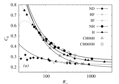
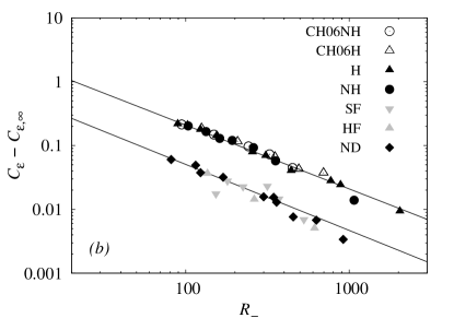
Figure 1: (a) Eq. (62) fitted to the different datasets H, NH, CH06H, CH06NH (free decay) and ND (stationary). Data from the stationary series SF and HF are shown for comparison purposes. The black lines refer to fits using Eq. (62) up to first order, while the gray lines use Eq. (62) up to second order in $1/R_{-}$. The error bars show one standard error. As can be seen, the respective asymptotes differ between the data sets H, NH, CH06H, CH06NH and ND, while data from series SF and HF is compatible with data from series ND. (b) Fit of the expression $C/R_{-}^{n}$ corresponding to eq. (62) after subtraction of the asymptote $C_{\varepsilon,\infty}$ on a logarithmic scale to the datasets H (free decay, top line) and ND (stationary, bottom line). Data from the series NH, CH06H, CH06NH, SF and HF are shown for comparison purposes. The resulting exponents are $n=1.00\pm 0.01$ for free decay and $n=1.00\pm 0.02$ for the stationary case.

IV.2 Stationary MHD turbulence

In this case measurements are taken after the simulations have reached a stationary state. The value of $C_{\varepsilon}$ and the corresponding statistics for each data point are calculated from time-series obtained by evolving the stationary simulations for a minimum of $9$ large-eddy turnover times, as specified in Tbl. 3. All runs of the series ND satisfy $k_{max}\eta_{mag,kin}\geqslant 1.37$ and as such are sufficiently resolved. The runs SF4, HF3 and HF4 are marginally resolved, and we point out that the fitting procedure only involved data obtained from the ND series. The data points obtained from the series SF and HF are included for comparison purposes. Further details of the stationary simulations are given in Tbl. 3. All helicities are initially negligible and remain so during the evolution of the simulations.

Figure 1 (a) shows error-weighted fits of Eq. (62) to DNS data obtained from series ND. As can be seen, Eq. (62) fits the data well, provided terms of second order in $R_{-}$ are included to accommodate the data points at low $R_{-}$. For $R_{-}>80$, it is sufficient to consider terms of first order in $R_{-}$ only. The power law scaling to first order in $R_{-}$ is shown in further detail in Fig. 1 (b), where a function of the form $C/R_{-}^{n}$ was fitted to data from series ND for $R_{-}>80$ after subtraction of the asymptote $C_{\varepsilon,\infty}$. The fit resulted in the value $n=1.00\pm 0.02$ for the exponent, thus confirming that Eq. (62) describes the variation of $C_{\varepsilon}$ at moderate to high $R_{-}$ well already at first order in $R_{-}$. This is similar to results in isotropic hydrodynamic turbulence, where the corresponding hydrodynamic equation ${C_{\varepsilon}}_{u}={C_{\varepsilon,\infty}}_{u}+C_{u}/R_{L}$ agreed well with the data for $R_{L}>80$ McComb et al. (2015a). In this context we point out that the lowest value of $R_{L}$ in Ref. McComb et al. (2015a) was $R_{L}=81.5$. For $R_{-}\leqslant 80$ we find the data to be consistent with Eq. (62) once terms of second order in $R_{-}$ are taken into account. However, it can be very difficult to extract two power laws clearly from numerical data, especially if the leading and the subleading coefficients are of opposite sign Biferale et al. (2004); Mitra et al. (2005). This is the case here, the subleading coefficient $D$ is always negative while the leading coefficient $C$ is always positive.

Figure 1 also shows that the result is independent of the forcing scheme, as the datasets obtained from simulations using the three different forcing functions are consistent with each other. This is likely to change if the strategy of energy input is fundamentally changed, for example if the helical content and/or the characteristic scale of the force are altered, or if an electromagnetic force is used. We will come back to this point in Sec. V. The independence of $C_{\varepsilon}$ of the forcing scheme established here only shows independence of the specific implementation of the forcing. The asymptote has been calculated to be $C_{\varepsilon,\infty}=0.223\pm 0.003$, where the error is obtained from the fit.

A comparison of the measured values for $C_{\varepsilon,\infty}$ obtained from the different simulation series is provided in Tbl. 4. Comparing the results from stationary and decaying simulations with the same level of helicities could shed some light on the effect of external forces in the context of nonuniversality. As such, we compare the measured value of $C_{\varepsilon,\infty}=0.223$ to the value calculated for the series of decaying simulations NH, which results in a difference of about $12\%$. Since $C_{\varepsilon,\infty}$ does not depend explicitly on the external forces, the difference between the measured values may originate from dynamical effects. In relation to the effect of initial cross- and magntic helicities on the value of $C_{\varepsilon,\infty}$ discussed in Sec. IV.1, we expect further variance in the measured value of $C_{\varepsilon,\infty}$ depending on the level of cross- and magnetic helicities of the external forces. As can be seen from a comparison of the curves shown in Fig. 1, the coefficient $C$ in Eq. (62) is not the same for the stationary and decaying cases. This is expected since $C^{\pm}$ and hence $C$ depend explicitly on the energy input, as can be seen from Eq. (58).

Series id	$C_{\varepsilon,\infty}$	$\sigma_{C_{\varepsilon,\infty}}$	description
H	0.241	0.008	decaying, helical
NH	0.265	0.013	decaying, nonhelical
CH06H	0.193	0.006	decaying, helical, cross-helical
CH06NH	0.268	0.005	decaying, nonhelical, cross-helical
ND	0.223	0.003	stationary, nonhelical
Ref. McComb et al. (2015a)	0.468	0.006	non-conducting, stationary

Table 4: Summary of measured values for the asymptotic dimensionless dissipation rate $C_{\varepsilon,\infty}$ from the different simulation series. For comparison the measured values from a series of DNSs of stationary isotropic hydrodynamic turbulence McComb et al. (2015a) are included. The error on $C_{\varepsilon,\infty}$ is denoted by $\sigma_{C_{\varepsilon,\infty}}$ and refers to the error obtained from the error-weighted fitting procedure.

Some further observations can be made from a comparison of the datasets concerning the variance of the magnetic and kinetic contributions, $\varepsilon_{mag}$ and $\varepsilon_{kin}$, to the total energy dissipation rate. The fractions $\varepsilon_{mag}/\varepsilon$ and $\varepsilon_{kin}/\varepsilon$ are given columns 8 and 9, respectively, of Tbls. 1-3 for the different datasets. For the series H and CH06H it can be seen that the kinetic dissipation fraction $\varepsilon_{kin}/\varepsilon$ grows with increasing $R_{-}$ (or $R_{L}$), of course at the expense of the magnetic dissipation fraction $\varepsilon_{mag}/\varepsilon$. The reason for this behaviour could be connected with the inverse cascade of magnetic helicity becoming more efficient at higher $R_{-}$ resulting in a higher residual inverse transfer of magnetic energy and thus slightly less magnetic energy to be dissipated at the small scales. This interpretation is supported by the observation that no such variation is present for the nonhelical series NH and CH06NH, where we measure $\varepsilon_{mag}/\varepsilon\simeq 0.6$ and $\varepsilon_{mag}/\varepsilon\simeq 0.4$ for all data points. For all four datasets corresponding to freely decaying MHD turbulence the magnetic dissipation fraction is always higher than the kinetic dissipation fraction, $\varepsilon_{mag}/\varepsilon>\varepsilon_{kin}/\varepsilon$.

The stationary datasets show yet a different variation of $\varepsilon_{mag}/\varepsilon$ and $\varepsilon_{kin}/\varepsilon$ with $R_{-}$. For $R_{-}<45$ we find $\varepsilon_{mag}/\varepsilon<\varepsilon_{kin}/\varepsilon$, while for $R_{-}>46$ the results are similar to free decay with $\varepsilon_{mag}/\varepsilon>\varepsilon_{kin}/\varepsilon$. The magnetic dissipation fraction increases with $R_{-}$ from $\varepsilon_{mag}/\varepsilon\simeq 0.3$ to $\varepsilon_{mag}/\varepsilon\simeq 0.7$, where it appears to reach a plateau. The fluctuating magnetic field is maintained by the velocity field fluctuations through a nonlinear dynamo process in the present DNSs of stationary MHD turbulence. Hence in the statistically stationary state $\varepsilon_{mag}$ is in balance with the dynamo term $\langle\bm{b}\cdot(\bm{b}\cdot\nabla)\bm{u}\rangle$, and the measured values of $\varepsilon_{mag}/\varepsilon$ and $\varepsilon_{kin}/\varepsilon$ imply that at lower Reynolds number the nonlinear dynamo is less efficient in maintaining small-scale magnetic field fluctuations than at higher Reynolds number. Similar conclusions have been reached in a study of the magnetic Prandtl number dependence of the ratio $\varepsilon_{kin}/\varepsilon_{mag}$ Brandenburg (2014), where the efficiency of the dynamo at different values of $Pm$ was linked to measured values of $\varepsilon_{kin}/\varepsilon_{mag}$.

V Conclusions

The behavior of the dimensionless dissipation coefficient $C_{\varepsilon}$ in homogeneous MHD turbulence with $Pm=1$ and no background magnetic field is well described by

$$C_{\varepsilon}=C_{\varepsilon,\infty}+\frac{C}{R_{-}}+\frac{D}{R_{-}^{2}}+O(R_{-}^{-3})\ .$$ (75)

This equation was derived from the energy balance equation for $\bm{z}^{\pm}$ in real space (the vKHE) by outer asymptotic expansions in powers of $1/R_{\mp}$, leading necessarily to a large-scale description of the behavior of the dimensionless dissipation rate. The approximative equation (75) has been shown to agree well with data obtained from medium to high resolution DNSs of both decaying MHD turbulence at the peak of dissipation and statistically steady MHD turbulence sustained by large-scale forcing. The measurements for $C_{\varepsilon,\infty}$ ranged from $0.193\leqslant C_{\varepsilon,\infty}\leqslant 0.268$ between the different series of simulations. Interestingly, the measured values of $C_{\varepsilon,\infty}$ for MHD are smaller than the measured value of $C_{\varepsilon,\infty}\simeq 0.5$ in hydrodynamic turbulence obtained both from numerical simulations and experiments Sreenivasan (1984); Jiménez et al. (1993); Wang et al. (1996); Yeung and Zhou (1997); Sreenivasan (1998); Cao et al. (1999); Pearson et al. (2002); Kaneda et al. (2003); Pearson et al. (2004); Donzis et al. (2005); Bos et al. (2007); Yeung et al. (2012); McComb et al. (2015a); Yeung et al. (2015), suggesting less energy transfer across scales in MHD turbulence compared to hydrodynamics.

The asymptote in the limit $R_{-}\to\infty$ originates from the sum of the nonlinear terms in the momentum and induction equations, that is, it measures the total transfer flux, which is expected to depend on the values of the ideal invariants. As predicted, the values of the respective asymptotes from the datasets differ, suggesting a dependence of $C_{\varepsilon,\infty}$ on different values of the helicities, and thus a connection to questions of universality in MHD turbulence. For maximally helical magnetic fields $C_{\varepsilon,\infty}$ is smaller than for nonhelical fields. This is expected from the inverse cascade of magnetic helicity. The dependence of $C_{\varepsilon,\infty}$ on the remaining ideal invariant, the cross-helicity, is more complex. Since $C_{\varepsilon,\infty}$ describes the flux of total energy across the scales, this flux is expected to diminish for increasing cross-helicity. This is indeed the case for helical magnetic fields, where $C_{\varepsilon,\infty}$ depends on the cross-helicity in the expected way. Surprisingly, for nonhelical magnetic fields $C_{\varepsilon,\infty}$ does not depend on the cross-helicity. This is consistent with the asymmetric effect of the cross-helicity on forward and inverse fluxes of total energy suggested by the analysis of triad interactions in Ref. Linkmann et al. (2016), where high levels of cross-helicity were found to quench forward transfer more than inverse transfer. A similar effect can be inferred from predictions obtained from statistical mechanics Frisch et al. (1975), where the simultaneous presence of cross- and magnetic helicities resulted in inverse transfers of both magnetic and kinetic energy. In this case, the forward flux of total energy should be lower than for all other cases, which is consistent with the numerical results presented here. Concerning stationary nonhelical MHD turbulence, we found that $C_{\varepsilon,\infty}$ differed by about $12\%$ from the value measured for nonhelical decaying turbulence (series NH) at the peak of dissipation. According to the results from the asymptotic analysis, there is no explicit dependence of $C_{\varepsilon,\infty}$ on the external force. As such, the difference in the measured value of $C_{\varepsilon,\infty}$ between the stationary and the decaying systems may be due to dynamical effects, which may be interpreted as further support for nonuniversal values of $C_{\varepsilon}$. The approach to the asymptote is predicted to differ between decaying and stationary systems due to the explicit dependence of the coefficient $C$ in Eq. (62) on the forcing. This is indeed observed in the simulations.

The numerical results showed that $C_{\varepsilon,\infty}$ is universal with respect to different forcing schemes applied to the same field in the same wavenumber range, thus confirming that the particular functional form and stochasticity of a large-scale force is irrelevant to the small-scale turbulent dynamics as long as the ideal invariants remain the same for the different forcing schemes. However, as mentioned in Sec. IV, this is expected to change if the strategy of energy input is changed. The effect of large-scale magnetic forcing on the scaling of $\varepsilon$ with different rms quantities was investigated recently Alexakis (2013). Numerical results showed that $\varepsilon\sim U^{3}/L_{\bm{f}_{u}}$ for a large region of parameter space even in the presence of electromagnetic forces. Only once the large-scale magnetic field became very strong a different scaling related to the dominance of magnetic shear over mechanical shear was found: $\varepsilon\sim BU^{2}/L_{\bm{f}_{b}}$. Differences may also be expected for forces applied at smaller scales. The analysis presented here relies on taking outer asymptotic expansions of all scale-dependent functions in the vKHE, including the energy input from the forcing. Here it was crucial to assume that the system was forced at the large scales, as the limit of infinite Reynolds number was defined as energy input at the lowest wavenumbers $k\to 0$ and removal of energy at the largest wavenumbers $k\to\infty$. This clearly precludes the application of the present analysis to situations where the system is forced at intermediate or small scales. Therefore, it can be expected that systems forced at intermediate scales deviate from the $1/R_{-}$-scaling of $C_{\varepsilon}$. For hydrodynamics, this is the case Doering (2009); Biferale et al. (2004); Mazzi and Vassilicos (2004). Furthermore, experimental and numerical results for nonstationary flows Valente et al. (2014); Vassilicos (2015) suggest even further variance possibly due to the influence of the time-derivative of the second-order structure function in the vKHE.

The results presented here were restricted to homogeneous MHD turbulence at $Pm=1$ without a mean magnetic field. In general, further variance in the measured value for $C_{\varepsilon,\infty}$ is expected depending on e.g. the magnetic Prandtl number Brandenburg (2014) or the influence of a background magnetic field. The presence of a background magnetic field, which leads to spectral anisotropy and the breakdown of the conservation of magnetic helicity Matthaeus and Goldstein (1982), will introduce several difficulties to be overcome when generalizing the analytical approach. The spectral flux will then depend on the direction of the mean field Wan et al. (2009, 2012) and a more generalized description and role for the magnetic helicity would be needed Berger (1997, 1999). Other questions concern the generalization of this approach to MHD flows with magnetic Prandtl numbers $Pm\neq 1$, the effect of compressive fluctuations or the influence of other vector field correlations on the dissipation rate and/or the approach to the asymptote as observed by Dallas and Alexakis Dallas and Alexakis (2013a).

VI Acknowledgments

We thank V. Dallas for useful discussions. A. B. acknowledges support from the UK Science and Technology Facilities Council, M. L. received support from the UK Engineering and Physical Sciences Research Council (EP/K503034/1) and E. E. G. was supported by a University of Edinburgh Physics and Astronomy Fellowship. This work has made use of the resources provided by the UK National Supercomputing facility ARCHER, (http://www.archer.ac.uk), made available through the Edinburgh Compute and Data Facility (ECDF,
http://www.ecdf.ed.ac.uk). The research leading to these results has received funding from the European Union’s Seventh Framework Programme (FP7/2007-2013) under grant agreement No. 339032.

Appendix A Gauge independence of Equation (9)

In order to prove that Eq. (9) is correct for an arbitrary choice of gauge, we first express the current density $\bm{j}$ in terms of the vector potential $\bm{a}$

$$\bm{j}=\nabla\times(\nabla\times\bm{a})=-\Delta\bm{a}+\nabla(\nabla\cdot\bm{a})\ ,$$ (76)

which holds in any gauge. In Fourier space this relation becomes

$$\hat{\bm{j}}=k^{2}\hat{\bm{a}}+i\bm{k}(i\bm{k}\cdot\hat{\bm{a}}),\$$ (77)

hence one obtains

$$\int_{\Omega}d\bm{k}\ \left\langle\frac{1}{k^{2}}\hat{\bm{j}}\cdot\hat{\bm{b}}^{*}\right\rangle=\int_{\Omega}d\bm{k}\ \left\langle\left(\hat{\bm{a}}+\frac{i\bm{k}}{k^{2}}(i\bm{k}\cdot\hat{\bm{a}})\right)\cdot\hat{\bm{b}}^{*}\right\rangle=\int_{\Omega}d\bm{k}\ \left\langle\hat{\bm{a}}\cdot\hat{\bm{b}}^{*}\right\rangle=H_{m}\ ,$$ (78)

since $\bm{b}$ is a solenoidal vector field. Equation (9) now follows by writing the Fourier coefficients of the magnetic field and the current density in the Elsässer formulation

$$\hat{\bm{b}}=\frac{\hat{\bm{z}}^{+}-\hat{\bm{z}}^{-}}{2}\qquad\mbox{and}\qquad\hat{\bm{j}}=i\bm{k}\times\hat{\bm{b}}=i\bm{k}\times\frac{\hat{\bm{z}}^{+}-\hat{\bm{z}}^{-}}{2}\ .$$ (79)

References

- Kolmogorov (1941) A. N. Kolmogorov, C. R. Acad. Sci. URSS 30, 301 (1941).
- Iroshnikov (1964) P. S. Iroshnikov, Soviet Astronomy 7, 566 (1964).
- Kraichnan (1965) R. H. Kraichnan, Phys. Fluids 8, 1385 (1965).
- Goldreich and Sridhar (1995) P. Goldreich and S. Sridhar, Astrophys. J. 438, 763 (1995).
- Boldyrev (2005) S. Boldyrev, ApJ 626, L37 (2005).
- Boldyrev (2006) S. Boldyrev, Phys. Rev. Lett. 96, 115002 (2006).
- Beresnyak and Lazarian (2006) A. Beresnyak and A. Lazarian, ApJL 640, L175 (2006).
- Mason et al. (2006) J. Mason, F. Cattaneo, and S. Boldyrev, Phys. Rev. Lett. 97, 255002 (2006).
- Gogoberidze (2007) G. Gogoberidze, Phys. Plasmas 14, 022304 (2007).
- Dallas and Alexakis (2013a) V. Dallas and A. Alexakis, Phys. Fluids 25, 105106 (2013a).
- Dallas and Alexakis (2013b) V. Dallas and A. Alexakis, Phys. Rev. E 88, 063017 (2013b).
- Wan et al. (2012) M. Wan, S. Oughton, S. Servidio, and W. H. Matthaeus, J. Fluid Mech. 697, 296 (2012).
- Schekochihin et al. (2008) A. A. Schekochihin, S. C. Cowley, and T. A. Yousef, in IUTAM Symposium on Computational Physics and New Perspectives in Turbulence, edited by Y. Kaneda (Springer, Berlin, 2008) pp. 347–354.
- Mininni (2011) P. D. Mininni, Annu. Rev. Fluid Mech. 43, 377 (2011).
- Grappin et al. (1983) R. Grappin, A. Pouquet, and J. Léorat, Astron. Astrophys. 126, 51 (1983).
- A. Pouquet and P. Mininni and D. Montgomery and A. Alexakis (2008) A. Pouquet and P. Mininni and D. Montgomery and A. Alexakis, in IUTAM Symposium on Computational Physics and New Perspectives in Turbulence, edited by Y. Kaneda (Springer, 2008) pp. 305–312.
- Beresnyak (2011) A. Beresnyak, Phys. Rev. Lett. 106, 075001 (2011).
- Boldyrev et al. (2011) S. Boldyrev, J. C. Perez, J. E. Borovsky, and J. J. Podesta, Astrophys. J. 741, L19 (2011).
- Grappin and Müller (2010) R. Grappin and W.-C. Müller, Phys. Rev. E 82, 026406 (2010).
- Lee et al. (2010) E. Lee, M. E. Brachet, A. Pouquet, P. D. Mininni, and D. Rosenberg, Phys. Rev. E 81, 016318 (2010).
- Servidio et al. (2008) S. Servidio, W. H. Matthaeus, and P. Dmitruk, Phys. Rev. Lett. 100, 095005 (2008).
- Frisch et al. (1975) U. Frisch, A. Pouquet, J. Léorat, and A. Mazure, J. Fluid Mech. 68, 769 (1975).
- Pouquet et al. (1976) A. Pouquet, U. Frisch, and J. Léorat, J. Fluid Mech. 77, 321 (1976).
- Pouquet and Patterson (1978) A. Pouquet and G. S. Patterson, J. Fluid Mech. 85, 305 (1978).
- Biskamp (1993) D. Biskamp, Nonlinear Magnetohydrodynamics., 1st ed. (Cambridge University Press, 1993).
- Alexakis (2013) A. Alexakis, Phys. Rev. Lett. 110, 084502 (2013).
- Sreenivasan (1984) K. R. Sreenivasan, Phys. Fluids 27, 1048 (1984).
- Sreenivasan (1998) K. R. Sreenivasan, Phys. Fluids 10, 528 (1998).
- McComb (2014) W. D. McComb, Homogeneous, Isotropic Turbulence: Phenomenology, Renormalization and Statistical Closures (Oxford University Press, 2014).
- McComb et al. (2015a) W. D. McComb, A. Berera, S. R. Yoffe, and M. F. Linkmann, Phys. Rev. E 91, 043013 (2015a).
- Yeung et al. (2015) P. K. Yeung, X. M. Zhai, and K. R. Sreenivasan, PNAS 112, 12633–12638 (2015).
- Jagannathan and Donzis (2016) S. Jagannathan and D. A. Donzis, J. Fluid Mech. 789, 669 (2016).
- Mininni and Pouquet (2009) P. D. Mininni and A. G. Pouquet, Phys. Rev. E. 80, 025401 (2009).
- Dallas and Alexakis (2014) V. Dallas and A. Alexakis, Astrophys. J. 788, L36 (2014).
- Linkmann et al. (2015) M. F. Linkmann, A. Berera, W. D. McComb, and M. E. McKay, Phys. Rev. Lett. 114, 235001 (2015).
- Politano and Pouquet (1998) H. Politano and A. Pouquet, Phys. Rev. E 57, R21 (1998).
- Elsässer (1950) W. M. Elsässer, Phys. Rev. 79, 183 (1950).
- Chandrasekhar (1951) S. Chandrasekhar, Proc. Roy. Soc. London. Series A 204, 435 (1951).
- Note (1) The scaling is ill-defined for the (measure zero) cases , which correspond to exact solutions to the MHD equations where the nonlinear terms vanish. Thus no turbulent transfer is possible, and these cases are not amenable to an analysis which assumes nonzero energy transfer Politano and Pouquet (1998).
- Novikov (1965) E. A. Novikov, Soviet Physics JETP 20, 1290 (1965).
- Lundgren (2002) T. S. Lundgren, Phys. Fluids 14, 638 (2002).
- Linkmann et al. (2016) M. F. Linkmann, A. Berera, M. E. McKay, and J. Jäger, J. Fluid Mech. 791, 61 (2016).
- Berera and Linkmann (2014) A. Berera and M. F. Linkmann, Phys. Rev. E 90, 041003(R) (2014).
- Linkmann (2016) M. Linkmann, Self-organisation in (magneto)hydrodynamic turbulence, Ph.D. thesis, University of Edinburgh (2016).
- Brandenburg (2001) A. Brandenburg, Astrophys. J. 550, 824 (2001).
- Dallas and Alexakis (2015) V. Dallas and A. Alexakis, Phys. Fluids 27, 045105 (2015).
- Sahoo et al. (2011) G. Sahoo, P. Perlekar, and R. Pandit, New Journal of Physics 13, 013036 (2011).
- McComb et al. (2015b) W. D. McComb, M. F. Linkmann, A. Berera, S. R. Yoffe, and B. Jankauskas, J. Phys. A: Math. Theor. 48, 25FT01 (2015b).
- Linkmann and Morozov (2015) M. F. Linkmann and A. Morozov, Phys. Rev. Lett. 115, 134502 (2015).
- Müller et al. (2012) W. C. Müller, S. K. Malapaka, and A. Busse, Phys. Rev. E 85, 015302 (2012).
- Malapaka and Müller (2013) S. K. Malapaka and W.-C. Müller, Astrophys. J. 778, 21 (2013).
- Linkmann and Dallas (2016) M. Linkmann and V. Dallas, Phys. Rev. E 94, 053209 (2016).
- (53) The data is publicly available, http://dx.doi.org/10.7488/ds/247.
- Biferale et al. (2004) L. Biferale, A. S. Lanotte, and F. Toschi, Phys. Rev. Lett. 92, 094503 (2004).
- Mitra et al. (2005) D. Mitra, J. Bec, R. Pandit, and U. Frisch, Phys. Rev. Lett. 94, 194501 (2005).
- Brandenburg (2014) A. Brandenburg, ApJ 791, 12 (2014).
- Jiménez et al. (1993) J. Jiménez, A. A. Wray, P. G. Saffman, and R. S. Rogallo, J. Fluid Mech. 255, 65 (1993).
- Wang et al. (1996) L.-P. Wang, S. Chen, J. G. Brasseur, and J. C. Wyngaard, J. Fluid Mech. 309, 113 (1996).
- Yeung and Zhou (1997) P. K. Yeung and Y. Zhou, Phys. Rev. E 56, 1746 (1997).
- Cao et al. (1999) N. Cao, S. Chen, and G. D. Doolen, Phys. Fluids 11, 2235 (1999).
- Pearson et al. (2002) B. R. Pearson, P. A. Krogstad, and W. van de Water, Phys. Fluids 14, 1288 (2002).
- Kaneda et al. (2003) Y. Kaneda, T. Ishihara, M. Yokokawa, K. Itakura, and A. Uno, Phys. Fluids 15, L21 (2003).
- Pearson et al. (2004) B. R. Pearson, T. A. Yousef, N. E. L. Haugen, A. Brandenburg, and P. A. Krogstad, Phys. Rev. E 70, 056301 (2004).
- Donzis et al. (2005) D. A. Donzis, K. R. Sreenivasan, and P. K. Yeung, J. Fluid Mech. 532, 199 (2005).
- Bos et al. (2007) W. J. T. Bos, L. Shao, and J.-P. Bertoglio, Phys. Fluids 19, 045101 (2007).
- Yeung et al. (2012) P. K. Yeung, D. A. Donzis, and K. R. Sreenivasan, J. Fluid Mech. 700, 5 (2012).
- Doering (2009) C. R. Doering, Annu. Rev. Fl. Mech. 41, 109 (2009).
- Mazzi and Vassilicos (2004) B. Mazzi and J. C. Vassilicos, J. Fluid Mech. 502, 65 (2004).
- Valente et al. (2014) P. C. Valente, R. Onishi, and C. B. da Silva, Phys. Rev. E 90, 023003 (2014).
- Vassilicos (2015) J. C. Vassilicos, Annu. Rev. Fluid Mech. 47, 95 (2015).
- Matthaeus and Goldstein (1982) W. H. Matthaeus and M. L. Goldstein, J. Geophys. Res. 87, 6011 (1982).
- Wan et al. (2009) M. Wan, S. Servidio, S. Oughton, and W. H. Matthaeus, Phys. Plasmas 16, 090703 (2009).
- Berger (1997) M. A. Berger, J. Geophys. Res. 102, 2637 (1997).
- Berger (1999) M. A. Berger, Plasma Physics and Controlled Fusion 41, B167 (1999).