A re-analysis of the NuSTAR and XMM-Newton broad-band spectrum of Ser X-1

Abstract

Context. High resolution X-ray spectra of neutron star Low Mass X-ray Binaries (LMXBs) in the energy range 6.4-6.97 keV, are often characterized by the presence of K$\alpha$ transition features of iron at different ionization stages. Since these lines are thought to originate by reflection of the primary Comptonization spectrum over the accretion disk, the study of these features allows us to investigate the structure of the accretion flow close to the central source. Thus, the study of these features gives us important physical information on the system parameters and geometry. Ser X-1 is a well studied LMXB which clearly shows a broad iron line. Several attempts to fit this feature as a smeared reflection feature have been performed on XMM-Newton, Suzaku, NuSTAR, and, more recently, on Chandra data, finding different results for the inner radius of the disk and other reflection or smearing parameters. For instance, Miller et al. (2013) have presented broad-band, high quality NuSTAR data of Ser X-1. Using relativistically smeared self-consistent reflection models, they find a value of R_in close to 1.0 R_ISCO (corresponding to 6 R_g, where R_g is the Gravitational radius, defined as usual R${}_{g}=GM/c^{2}$), and a low inclination angle of less than $\sim 10^{\circ}$.

Aims. The aim of this paper is to probe to what extent the choice of reflection and continuum models (and uncertainties therein) can affect the conclusions about the disk parameters inferred from the reflection component. To this aim we re-analyze all the available public NuSTAR and XMM-Newton which have the best sensitivity at the iron line energy observations of Ser X-1. Ser X-1 is a well studied source, its spectrum has been observed by several instruments, and is therefore one of the best sources for this study.

Methods. We use slightly different continuum and reflection models with respect to those adopted in literature for this source. In particular we fit the iron line and other reflection features with self-consistent reflection models as reflionx (with a power-law illuminating continuum modified with a high energy cutoff to mimic the shape of the incident Comptonization spectrum) and rfxconv. With these models we fit NuSTAR and XMM-Newton spectra yielding consistent spectral results.

Results. Our results are in line with those already found by Miller et al. (2013) but less extreme. In particular, we find the inner disk radius at $\sim 13\,R_{g}$ and an inclination angle with respect to the line of sight of $\sim 27^{\circ}$. We conclude that, while the choice of the reflection model has little impact on the disk parameters, as soon as a self-consistent model is used, the choice of the continuum model can be important in the precise determination of the disk parameters from the reflection component. Hence broad-band X-ray spectra are highly preferable to constrain the continuum and disk parameters.

1 Introduction

X-ray spectra emitted by Low Mass X-Ray Binaries (LMXBs) of the atoll class (Hasinger & van der Klis 1989) are usually characterized by two states of emission: the soft and the hard state. During soft states the spectrum can be well described by a soft thermal component, usually a blackbody or a disk multi-color blackbody, possibly originated from the accretion disk, and a harder component, usually a saturated Comptonization spectrum. In some cases, a hard power-law tail has been detected in the spectra of these sources during soft states both in Z sources (Di Salvo et al. 2000), and in atoll sources (e.g., Piraino et al. 2007), usually interpreted as Comptonization off a non-thermal population of electrons. On the other hand, during hard states the hard component of the spectrum can be described by a power law with high energy cutoff, interpreted as unsaturated Comptonization, and a weaker soft blackbody component (e.g., Di Salvo et al. 2015). The hard component is generally explained in terms of inverse Compton scattering of soft photons, coming from the neutron star surface and/or the inner accretion disk, by hot electrons present in a corona possibly located in the inner part of the system, surrounding the compact object (D’Aì et al. 2010).

In addition to the continuum, broad emission lines in the range 6.4-6.97 keV are often observed in the spectra of LMXBs (see e.g. Cackett et al. 2008; Pandel et al. 2008; D’Aì et al. 2009, 2010; Iaria et al. 2009; Di Salvo et al. 2005, 2009; Egron et al. 2013; Di Salvo et al. 2015). These lines are identified as K$\alpha$ transitions of iron at different ionization states and are thought to originate from reflection of the primary Comptonization spectrum over the accretion disk. These features are powerful tools to investigate the structure of the accretion flow close to the central source. In particular, important information can be inferred from the line width and profile, since the detailed profile shape is determined by the ionization state, geometry and velocity field of the emitting plasma (see e.g. Fabian et al. 1989). Indeed, when the primary Comptonization spectrum illuminates a colder accretion disk, other low-energy discrete features (such as emission lines and absorption edges) are expected to be created by photoionization and successive recombination of abundant elements in different ionizations states as well as a continuum emission caused by direct Compton scattering of the primary spectrum off the accretion disk. All these features together form the so-called reflection spectrum, and the whole reflection spectrum is smeared by the velocity-field of the matter in the accretion disk.

Ser X-1 is a persistent accreting LMXB classified as an atoll source, that shows type I X-ray bursts. The source was discovered in 1965 by Friedman et al. (1967). Li et al. (1976) firstly discovered type-I X-ray bursts from this source that was therefore identified as an accreting neutron star. Besides type-I bursts with typical duration of few seconds (Balucinska & Czerny 1985), a super-burst of the duration of about 2 hours has also been reported (Cornelisse et al. 2002). Recently Cornelisse et al. (2013), analyzing spectra collected by GTC, detected a two-hours periodicity. They tentatively identified this periodicity as the orbital period of the binary and hence proposed that the secondary star might be a main sequence K-dwarf.

Church & Balucińska-Church (2001) have performed a survey of LMXBs carried out with the ASCA satellite. The best-fit model used by these authors to fit the spectrum of Ser X-1 was a blackbody plus a cutoff power-law with a Gaussian iron line. Oosterbroek et al. (2001) have analyzed two simultaneous observations of this source collected with BeppoSAX and RXTE. The authors fitted the broad-band (0.1-200 keV) BeppoSAX spectrum with a model consisting of a disk blackbody, a reflection component described by the XSPEC model pexrav, and a Gaussian line. However, in that case the improvement in $\chi^{2}$ with respect to a model consisting of a blackbody, a Comptonization spectrum modeled by compST, and a Gaussian was not significant, and therefore it was not possible to draw any definitive conclusion about the presence of a reflection continuum.

Bhattacharyya & Strohmayer (2007) carried out the analysis of three XMM-Newton observations of this system. They managed to fit the EPIC/pn spectrum with a model consisting of disk blackbody, a Comptonization continuum modeled with compTT and a diskline, i.e. a Gaussian line distorted and smeared by the Keplerian velocity field in the accretion disk (Fabian et al. 1989). They found strong evidence that the Fe line has an asymmetric profile and therefore that the line originates from reflection in the inner rim of the accretion disk. Fitted with a Laor profile (Laor 1991), the line shape gave an inner disk radius of $4-5\,R_{g}$ or $16\,R_{g}$ (depending from the observation) and an inclination angle to the binary system of $40-50^{\circ}$. Cackett et al. (2008), from data collected by SUZAKU, performed a study of the iron line profiles in a sample of three LMXBs including Ser X-1. From the analysis of XIS and PIN spectra, they found a good fit of the broad-band continuum using a blackbody, a disk blackbody and a power-law. Two years later Cackett et al. (2010) re-analyzed XMM-Newton and SUZAKU data of a sample of 10 LMXBs that includes Ser X-1, focusing on the iron line - reflection emission. In particular, for Ser X-1, they analyzed 4 spectra: three Epic-PN spectra obtained with XMM-Newton and one obtained with the XIS and the PIN instruments on board of SUZAKU. Initially, they fitted the spectra of the continuum emission using a phenomenological model, consisting of a blackbody, a disk-blackbody and a power-law. Then, they started the study of the Fe line adding first a diskline component and after a reflection component convolved with rdblur (that takes into account smearing effects due to the motion of the emitting plasma in a Keplerian disk). They obtained different results for the smearing parameters both for different observations and for different models used on the same observation. For sake of clarity these results are summarized in Table 1.

Miller et al. (2013) analyzed two NuSTAR observations carried out on July 2013. They fitted the continuum emission using a model consisting of a blackbody, a disk blackbody and a power-law. With respect to this continuum model, evident residuals were present around 6.40-6.97 keV, suggesting the presence of a Fe line. Therefore they added a kerrdisk component to the continuum to fit the emission line, taking into account a possible non-null spin parameter for the neutron star. They also tried to fit the reflection spectrum (i.e. the iron line and other expected reflection features) with the self-consistent reflection model reflionx, a modified version of reflionx calculated for a blackbody illuminating spectrum, convolved with the kerrconv component. The addition of the reflection component gave a significant improvement of the fit. In most cases the best fit gave low inclination angles (less than $\sim 10^{\circ}$), in agreement with recent optical observations (Cornelisse et al. 2013), inner disk radii compatible with the Innermost Stable Circular Orbit (ISCO), corresponding to about 6 Rg for small values of the spin parameter, a ionization parameter $\log\xi\sim 2.3-2.6$, and a slight preference for an enhanced iron abundance. The fit resulted quite insensitive to the value of the adimensional spin parameter, a, of the neutron star.

More recently, Chiang et al. (2016) analysed a recent 300 ks Chandra/HETGS observation of the source performed in the ”continuous clocking” mode and thus free of photon pile-up effects. They fitted the continuum with a combination of multicolor disk blackbody, blackbody and power-law. The iron line was found significantly broader than the instrumental energy resolution and fitting this feature with a diskline instead of a broad Gaussian gave a significant improvement of the fit. They also tried self-consistent reflection models, namely the reflionx model with a power-law continuum as illuminating source and xillver (see e.g. García et al. 2013), to describe the iron line and other reflection features, yielding consistent results. In particular, this analysis gave a inner radius of $\sim 7-8$ R_g and an inclination angle of about 30 deg.

As described above, different continuum models were used to fit the spectrum of Ser X-1 observed with various instruments at different times. In Table 1 we summarize the results of the spectral analysis of this source obtained from previous studies, and in particular the results obtained for the iron line and the reflection model. Quite different values have been reported for the inclination angle (from less than 10 deg to about 40 deg), for the inner disk radius (from 4 to more than 100 R_g) and for the iron line centroid energy and/or the ionization parameter $\log\xi$ indicating that the disk is formed by neutral or very highly ionized plasma.

In this paper we re-analyzed all the available public NuSTAR observations of Ser X-1, fitting the iron line and other reflection features with both phenomenological and self-consistent reflection models. These data were already analysed by Miller et al. (2013) using a different choice of the continuum and reflection models. We compare these results with those obtained from three XMM-Newton observations (already analyzed by Bhattacharyya & Strohmayer 2007) fitted with the same models. We choose to re-analyse NuSTAR and XMM-Newton spectra because these instruments provide the largest effective area available to date, coupled with a moderately good energy resolution, at the iron line energy, and a good broad-band coverage. Moreover, the source showed similar fluxes during the NuSTAR and XMM-Newton observations. Note also that NuSTAR is not affected by pile-up problems in the whole energy range. The spectral results obtained for NuSTAR and XMM-Newton are very similar to each other and the smearing parameters of the reflection component are less extreme than those found by Miller et al. (2013), and in good agreement with the results obtained from the Chandra observation (Chiang et al. 2016). In particular we find an inner disk radius in the range $10-15\,R_{g}$ and an inclination angle with respect to the line of sight of $25-30^{\circ}$.

2 Observations and Data Reduction

In this paper we analyze data collected by the NuSTAR satellite. Ser X-1 has been observed twice with NuSTAR, obsID: 30001013002 (12-JUL-2013) and obsID: 30001013004 (13-JUL-2013). The exposure time of each observation is about 40 ksec. The data were extracted using NuSTARDAS (NuSTAR Data Analysis Software) v1.3.0. Source data have been extracted from a circular region with 120” radius whereas the background has been extracted from a circular region with 90” radius in a region far from the source. First, we run the ”nupipeline” with default values of the parameters as we aim to get ”STAGE 2” events clean. Then spectra for both detectors, FPMA and FPMB, were extracted using the ”nuproducts” command. Corresponding response files were also created as output of nuproducts. A comparison of the FPMA and FPMB spectra, indicated a good agreement between them. To check this agreement, we have fitted the two separate spectra with all parameters tied to each other but with a constant multiplication factor left free to vary. Since the value of this parameter is $1.00319\pm 0.00145$, our assumption is basically correct. Following the same approach described in Miller et al. (2013), we have therefore created a single added spectrum using the ”addascaspec” command. A single response file has been thus created using ”addrmf”, weighting the two single response matrices by the corresponding exposure time. In this way, we obtain a summed spectrum for the two NuSTAR observations and the two NuSTAR modules. We fitted this spectrum in the 3-40 keV energy range, where the emission from the source dominates over the background.

We have also used non-simultaneous data collected with XMM-Newton satellite on March 2004. The considered obsID are 0084020401, 0084020501 and 0084020601. All observations are in Timing Mode and each of them has a duration of $\sim$ 22 ksec. We extracted source spectra, background spectra and response matrices using the SAS (Science Analysis Software) v.14 setting the parameters of the tools accordingly. We produced a calibrated photon event file using reprocessing tools ”epproc” and ”rgsproc” for PN and RGS data respectively. We also extracted the MOS data; these were operated in uncompressed timing mode. However, the count rate registered by the MOS was in the range $290-340$ c/s, which is above the threshold for avoiding deteriorated response due to photon pile-up. The MOS spectra indeed show clear signs of pile-up and we preferred not to include them in our analysis, since these detectors cover the same energy range of the PN.

Before extracting the spectra, we filtered out contaminations due to background solar flares detected in the 10-12 keV Epic PN light-curve. In particular we have cut out about 600 sec for obsID 0084020401, about 800 sec for obsID 0084020501 and finally about 1600 sec for obsID 0084020601. In order to remove the flares, we applied time filters by creating a GTI file with the task ”tabgtigen”. In order to check for the presence of pile-up we have run the task ”epatplot” and we have found significant contamination in each observation. The count-rate registered in the PN observations was in the range 860-1000 c/s that is just above the limit for avoiding contamination by pile-up. Therefore, we extracted the source spectra from a rectangular region (RAW X$\geq$26) and (RAW X$\leq$46) including all the pixels in the y direction but excluding the brightest columns at RAW X = 35 and RAW X = 36. This reduced significantly the pile up (pile up fraction below a few percent in the considered energy range).

We selected only events with PATTERN $\leq$ 4 and FLAG$=$0 that are the standard values to remove spurious events. We extracted the background spectra from a similar region to the one used to extract the source photons but in a region away from the source included between (RAWX$\geq$1) and (RAWX$\leq$6 ). Finally, for each observation, using the task ’rgscombine’ we have obtained the added source spectrum RGS1+RGS2, the relative added background spectrum along with the relative response matrices. We have fitted RGS spectrum in the 0.35-1.8 keV energy range, whereas the Epic-PN in the 2.4-10 keV energy range.

Spectral analysis has been performed using XSPEC v.12.8.1 (Arnaud 1996). For each fit we have used the phabs model in XSPEC to describe the neutral photoelectric absorption due to the interstellar medium with photoelectric cross sections from Verner et al. (1996) and element abundances from Wilms et al. (2000). For the NuSTAR spectrum, which lacks of low- energy coverage up to 3 keV, we fixed the value of the equivalent hydrogen column, $N_{H}$, to the same value adopted by Miller et al. (2013), namely N${}_{H}\,=4\times 10^{21}$ cm^-2 (Dickey & Lockman 1990), while for the XMM-Newton spectrum we left this parameter free to vary in the fit, finding a slightly higher value (see Tab. 2 and 3). As a further check, we have fitted the NuSTAR spectrum fixing N_H to the same value found for the XMM spectrum, but the fit parameters did not change significantly.

3 Spectral Analysis

3.1 NuSTAR spectral analysis

The NuSTAR observations caught the source in a high-luminosity ($\sim 10^{38}$ erg/s, Miller et al. (2013)) state, therefore most probably in a soft state. As seen in other similar atoll sources, the spectrum of Ser X-1 is characterized by a soft component (i.e. blackbody), interpreted as thermal emission from the accretion disk, a hard component (i.e. a Comptonization spectrum), interpreted as saturated Comptonization from a hot corona, and often by the presence of a broad iron emission line at $6.4-6.97$ keV depending on the iron ionization state. We used the Comptonization model nthComp (Życki et al. 1999) in XSPEC, with a blackbody input seed photon spectrum, to fit the hard component. We used a simple blackbody to describe the soft component. Substituting the blackbody with a multicolor disk blackbody, diskbb in XSPEC, gives a similar quality fit and the best-fit parameters do not change significantly.

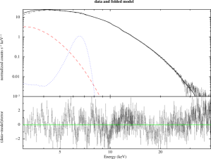
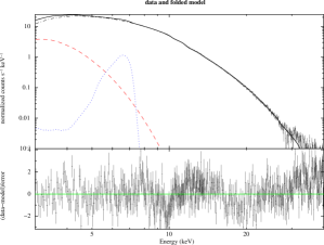
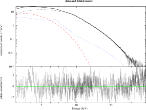
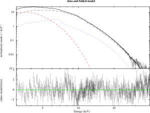
Figure 1: NuSTAR spectra of Ser X-1 and best-fitting model together with residuals in units of sigma for the corresponding model. These are: Top left: ’gauss’ — Top right: ’diskline’ — Bottom left: ’rdb-reflio’ — Bottom right: ’rdb-rfxconv’. Dashed lines indicate the black-body component, dotted lines indicate the reflection components (i.e. the Gaussian or Diskline profile for the iron line, top panels, or the self-consistent reflection component, bottom panels, respectively), and the dashed-dotted lines indicate the comptonized component.

To fit the iron line we first tried simple models such as a Gaussian profile or a diskline (Fabian et al. 1989). The best-fit parameters, obtained using alternatively a Gaussian or diskline profile, are in good agreement with each other (see Tab. 2). Using a diskline instead of a Gaussian profile we get an improvement of the fit corresponding to $\Delta\chi^{2}=54$ for the addition of two parameters. Spectra, along with the best-fit model and residuals are shown in Fig.1. In both cases, the fit results are poor (the relative null hypothesis probability is $2.8\times 10^{-8}$; the reduced $\chi^{2}\,$ are still relatively large, and evident residuals are present, especially above 10 keV, see Fig.1).

In order to fit the residuals at high energy, we added a powerlaw component (a hard tail) to all the models described above. A hard power-law tail is often required to fit high-energy residuals of atoll sources in the soft state (see e.g. Pintore et al. 2015, 2016; Iaria et al. 2001, 2002), and this component may also be present in the spectrum of Ser X-1 (see Miller et al. 2013). Unless it is specified otherwise, for every fit, we froze the power-law photon index to the value found by Miller et al. (2013) for Ser X-1, that is 3.2. The new models are now called gauss-pl and diskline-pl, respectively. The new best fit parameters are reported in Tab 2. While the best-fit parameters do not change significantly with the addition of this component, we get an improvement of the fit corresponding to a reduction of the $\chi^{2}$ by $\Delta\chi^{2}=123$ (for the model with a Gaussian line profile) and $\Delta\chi^{2}=113$ (for the model with a diskline profile) for the addition of one parameter, respectively. The probabilities of chance improvement of the fit are $8.5\times 10^{-24}$ and $8.6\times 10^{-23}$, respectively. Some residuals are still present between 10 and 20 keV probably caused by the presence of an unmodeled Compton hump. Note that the soft blackbody component remains significant even after the addition of the power-law component. If we eliminate this component from the fitting model we get a worse fit, corresponding to a decrease by $\Delta\chi^{2}=245$ for the addition of two parameters when the soft component is included in the fit and a probability of chance improvement of the fit of $\sim 3\times 10^{-44}$.

3.2 Reflection models

We have also tried to fit the NuSTAR spectrum of Ser X-1 with more sophisticated reflection models, performing a grid of fit with self-consistent models such as reflionx or rfxconv. Reflionx and rfxconv models both include the reflection continuum, the so called Compton hump caused by direct Compton scattering of the reflected spectrum, and discrete features (emission lines and absorption edges) for many species of atoms at different ionization stages (Ross & Fabian 2005; Kolehmainen et al. 2011).

The reflionx model depends on 5 parameters, that are the abundance of iron relative to the solar value, the photon index of the illuminating power-law spectrum ($\Gamma$, ranging between 1.0 to 3.0), the normalization of reflected spectrum, the redshift of the source, and the ionization parameter $\xi=L_{X}/(n_{e}r^{2})$ where $L_{X}$ is the X-ray luminosity of the illuminating source, $n_{e}$ is the electron density in the illuminated region and $r$ is the distance of the illuminating source to the reflecting medium. When using reflionx, which uses a power-law as illuminating spectrum, in order to take into account the high-energy roll over of the Comptonization spectrum, we have multiplied it by a high-energy cutoff, highecut, with the folding energy E_fold set to 2.7 times the electrons temperature kT_e and the cutoff energy E_cutoff tied to 0.1 keV. In this way we introduce a cutoff in the reflection continuum, which otherwise resembles a power-law. The cut-off energy fixed at 2.7 times the electron temperature of the Comptonization spectrum (assumed to be similar to a blackbody spectrum), is appropriate for a saturated Comptonization (see e.g. Egron et al. 2013). To fit the Comptonization continuum we used the nthComp model. Moreover we fixed the photon index of the illuminating spectrum, $\Gamma$, to that of the nthComp component. We stress that in our analysis we use a different reflionx reflection model with respect to that used by Miller et al. (2013). In fact we used a model that assumes an input power-law spectrum as the source of the irradiating flux modified, in order to mimic the nthcomp continuum, by introducing the model component highecut. Miller et al. (2013) instead used a modified version of reflionx calculated for a blackbody input spectrum, since that component dominates their phenomenological continuum.

rfxconv is an updated version of the code in Done & Gierliński (2006), using Ross & Fabian (2005) reflection tables. This is a convolution model that can be used with any input continuum and has therefore the advantage to take as illuminating spectrum the given Comptonization continuum. It depends on 5 parameters: the relative reflection fraction (rel-refl defined as $\Omega/2\pi$, namely as the solid angle subtended by the reflecting disk as seen from the illuminating corona in units of $2\pi$), the cosine of the inclination angle, the iron abundance relative to the Solar value, the ionization parameter Log $\xi$ of the accretion disk surface, and the redshift of the source.

Due to its high velocities, the radiation re-emitted from the plasma located in the inner accretion disk undergoes to Doppler and relativistic effects (which smears the whole reflection spectrum). In order to take these effects into account we have convolved the reflection models with the rdblur component (the kernel of the diskline model), which depends on the values of the inner and outer disk radii, in units of the Gravitational radius ($R_{g}=GM/c^{2}$), the inclination angle of the disk (that was kept tied to the same value used for the reflection model), and the emissivity index, Betor, that is the index of the power-law dependence of the emissivity of the illuminated disk (which scales as $r^{Betor}$). Finally, we have also considered the possibility that neutron star has a spin. In this case, the reflection component has been convolved with the Kerrconv component (Brenneman & Reynolds 2006) that through its adimensional spin parameter ’a’ allowed us to implement a grid of models exploring different values of ’a’ (see Appendix A). For this model there is also the possibility to fit the emissivity index of the inner and outer part of the disk independently, although in our fits we used the same emissivity index for the whole disk. For all the fits we have fixed the values of R_out to 2400 $R_{g}$, the iron abundance to solar value, Fe/solar = 1, and the redshift of the source to 0. The best fit parameters are reported in Tab 2–5.

We started to fit the data adding a reflection component, reflionx or rfxconv, convolved with the blurring component rdblur, to the continuum model given by the blackbody and the nthcomp components (models are called rdb-reflio and rdb-rfxconv, respectively). Fit results for both models are acceptable, with $\chi_{red}^{2}\,$ close to 1.09. There are a few differences between the best-fit parameters of the rdb-reflio model with respect to those of the rdb-rfxconv model. In particular the rdb-rfxconv model gives a lower value of R_in, while the rdb-reflio model gives a higher ionization parameter (although with a large uncertainty). Spectra, along with the best-fit model and residuals are reported in Fig.1. The residuals that are very similar for the two models, apart for the 8-10 keV energy range where rdb-reflio model shows flatter residuals than rdb-rfxconv model (see Fig. 1).

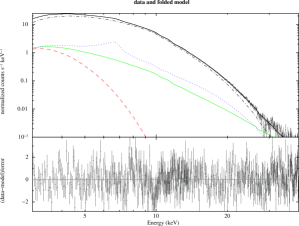
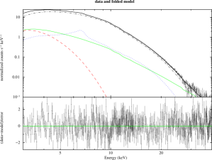
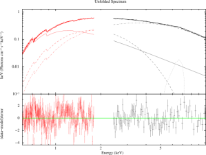
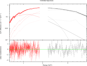
Figure 2: Top panels: NuSTAR spectra of Ser X-1 and best-fitting model together with residuals in units of sigma for the corresponding model. These are: Top left: ’rdb-reflio-pl’ — Top right: ’rdb-rfxconv-pl’. Bottom panels: XMM-Newton spectra and best-fitting model together with residuals in units of sigma for the corresponding model. These are: Bottom left: ’diskline-pl-xmm’ — Bottom right: ’rdb-rfxconv-pl-xmm’. For clarity only the first XMM-Newton observation is shown. Dashed lines indicate the black-body component, dotted lines indicate the reflection components (i.e. the Diskline profile for the iron line or the self-consistent reflection component), the solid line indicates the power-law component, and the dashed-dotted lines indicate the comptonized component.

As before, we also tried to add a power-law component to the models obtained by the convolution of the blurring component (rdblur) with the two different reflection components (rfxconv or reflionx). The two new models are called rdb-rfxconv-pl and rdb-reflion-pl, respectively. In both cases we get a significant improvement of the fit, with $\Delta\chi^{2}=90$ for the addition of two parameters and $\Delta\chi^{2}=66$ for the addition of one parameter, respectively. In these cases, an F-test yields a probability of chance improvement of $3.1\times 10^{-15}$ for rdb-reflion-pl and $6.1\times 10^{-19}$ for rdb-rfxconv-pl model, respectively. Spectra, along with best-fit model and residuals are reported in Fig. 2, whereas values of the best-fit parameters are listed in Tab. 3. Residuals are now flat (see plots reported in upper panels of Fig. 2). Note also that in this way we get more reasonable values of the best-fit parameters, especially for the ionization parameter, $\log\xi$, which is around 2.7 for both models, in agreement with the centroid energy of the iron line at about 6.5 keV, and well below 3.7 (a ionization parameter $\log\xi\sim 3.7$ would imply that the matter of the accretion disk would be fully ionized).

In summary, the best fit of the NuSTAR spectrum of Ser X-1 is obtained fitting the continuum with a soft blackbody component, a Comptonization spectrum, and a hard power-law tail and fitting the reflection features with the rfxconv model smeared by the rdblur component, since the fitting results are quite insensitive to the value of the spin parameter a (see Appendix A). This fit, corresponding to a $\chi^{2}(dof)=912.5(911)$, gives a blackbody temperature of $\simeq 0.54$ keV, a temperature of the seed photons for the Comptonization of $\simeq 0.93$ keV, an electron temperature of the Comptonizing corona of $\simeq 2.70$ keV and a photon index of the primary Comptonized component of $\simeq 2.17$, whereas the photon index of the hard power-law tail is steeper, around 3.2. The reflection component gives a reflection amplitude (that is the solid angle subtended by the accretion disk as seen from the Comptonizing corona) of $\simeq 0.24$ and a ionization parameter of $\log\xi\simeq 2.7$. The smearing of the reflection component gives an inner disk radius of $R_{in}$ ranging between 10 and 16 $R_{g}$, and inclination angle of the disk with respect to the line of sight of $i\simeq 27^{\circ}$, and the emissivity of the disk scaling as $\propto r^{-2.6\pm 0.2}$. Note that the Compton hump is highly significant. To evaluate its statistical significance we can compare the best fit obtained with the model diskline-pl with the best fit given by the model rdb-rfxconv-pl (the main difference between the two models is in fact that rfxconv contains the reflection continuum and diskline does not). Using rfxconv instead of diskline we get a decreases of the $\chi^{2}$ by $\Delta\chi^{2}=87$ for the addition of 1 parameter and an F-test probability of chance improvement of $8\times 10^{-20}$, which is statistically significant.

3.3 XMM-Newton Spectral Analysis

We have also carried out the analysis of XMM-Newton observations of Ser X-1. A previous study, based only on the PN data analysis, has been reported by Bhattacharyya & Strohmayer (2007). We updated the analysis by performing the fit of the RGS spectra in the 0.35–1.8 keV energy range and the PN spectra in the 2.4–10 keV energy range. Following the same approach used for the analysis on NuSTAR data, we assumed a continuum model composed of a blackbody, a hard power-law and the nthComp component. In addition to the continuum components described above, we have also detected several discrete features present in all RGS spectra, both in absorption and in emission that were supposed to be of instrumental origin by Bhattacharyya & Strohmayer (2007). The energies of the most intense features detected in our spectra lie between 0.5 keV and 0.75 keV. To fit these features we have therefore added three additional gaussians to our model: two absorption lines at 0.528 keV and at 0.714 keV, respectively, and one in emission at 0.541 keV. The identification of these lines is not straightforward. The 0.528 keV energy is close to the neutral O K$\alpha$ line, expected at a rest frame energy of 0.524 keV, while the 0.541 keV emission line is close to the expected energy of the O I edge at 0.538 keV. These two lines may be therefore instrumental features caused by a miscalibration of the neutral O edge in the RGS. The other absorption line at 0.714 keV is close to the O VII absorption edge expected at a rest-frame energy of 0.739 keV. Given that the identification of these lines is uncertain, we will not discuss them further in the paper. To this continuum we first added a diskline (model called diskline-pl-xmm, see Table 2) to fit the iron line profile. Then we fitted the spectra substituting the diskline with the self-consistent reflection model that gave the best fit to the NuSTAR data, that is ’rfxconv’, convolved with the smearing component ’rdblur’ (model called rdb-rfxconv-pl-xmm, results are reported in Table 3).

We have performed the fit of the spectrum obtained from these three observations simultaneously, tying parameters of the RGS with the all parameters of the PN from the same observation. The spectra of the three XMM observations are very similar with each other, except for the soft black body temperature that was left free to vary in different datasets. Values of the best-fit parameters of the model diskline-pl-xmm result to be in good agreement with what we have found from the fit of the NuSTAR spectra with the same model.

We have also performed the fit with a model including the reflection component rfxconv, called rdb-rfxconv-pl-xmm. As before, in order to take into account structures visible in the RGS spectra, we have added three gaussians to the model. As before we have tied parameters of the RGS to the corresponding parameters of the PN from the same observation except for the parameter kT_bb that was left free to vary among the three observations. Note also that for the these fits the inclination angle is fixed to the corresponding values we found from the NuSTAR spectra. Results are reported in Table 3, and are in good agreement with those obtained for the NuSTAR spectrum.

4 Discussion

Ser X-1 is a well studied LMXB showing a broad emission line at $6.4-6.97$ keV interpreted as emission from iron at different ionization states and smeared by Doppler and relativistic effects caused by the fast motion of matter in the inner accretion disk. Moderately high energy resolution spectra of this source have been obtained from XMM-Newton, Suzaku, NuSTAR, and Chandra. However, as described in Sec. 1, spectral results for the reflection component are quite different for different observations or for different models used to fit the continuum and/or the reflection component. While spectral differences in different observations may be in principle justified by intrinsic spectral variations of the source, differences caused by different continuum or reflection models should be investigated in detail in order to give a reliable estimate of the parameters of the system. For instance, in a recent NuSTAR observation analyzed by Miller et al. (2013), assuming a modified version of reflionx calculated for a black-body input spectrum, the authors report a significant detection of a smeared reflection component in this source, from which they derive an inner radius of the disk broadly compatible with the disk extending to the ISCO (corresponding to 6 Rg in the case $a=0$) and an inclination angle with respect to the line of sight $<10^{\circ}$. On the other hand, Chiang et al. (2016), analysing a recent 300 ks Chandra/HETGS observation of the source obtained a high-resolution X-ray spectrum which gave a inner radius of $R_{in}\sim 7-8\,R_{g}$ and an inclination angle of $\sim 30^{\circ}$.

In this paper we analyzed all the available NuSTAR and XMM-Newton observations of Ser X-1. These observations have been already analyzed by Miller et al. (2013) and Bhattacharyya & Strohmayer (2007), respectively, who used different continuum and reflection models and report different results for the reflection component. The same XMM-Newton observations have also been analyzed by Cackett et al. (2010) who also report different results for the reflection component, with higher inner disk radii (between 15 and more than $45\,R_{g}$) and quite low inclinations angles ($<10^{\circ}$) when using a blurred reflection model, and inclination angle between 10 and $35^{\circ}$ when using a diskline component to fit the iron line profile (see Tab. 1 for more details). We have shown that we can fit the NuSTAR and XMM-Newton spectra independently with the same continuum model and with a phenomenological model (i.e. diskline) or a self-consistent reflection model (i.e. reflionx or rfxconv) for the reflection component, finding in all our fit similar (compatible within the associated uncertainties) smearing parameters for the reflection component.

To fit these spectra we have used a continuum model composed by a blackbody component (bbody) and a comptonization continuum (nthcomp), which has been widely used in literature to fit the spectra of neutron star LMXBs both in the soft and in the hard state (see e.g. Egron et al. 2013). With respect to the continuum model used by Miller et al. (2013) we have substituted one of the two blackbody components, the hottest one, with a Comptonization spectrum. Since this component gives the most important contribution to the source flux, especially above 5 keV, we have subsequently used this component as the source of the reflection spectrum. In all our fit the addition of a hard power-law component, with a photon index $\sim 3$ significantly improved the fit. The presence of a hard power-law component is often found in the spectra of bright LMXBs in the soft state (see e.g. Piraino et al. 2007; Pintore et al. 2015, 2016), and has been interpreted as comptonization of soft photons off a non-thermal population of electrons (see e.g. Di Salvo et al. 2000).

To fit the reflection component, which is dominated by a prominent iron line, we have first used a phenomenological model consisting of a Gaussian line or a diskline, with a diskline providing a better fit than a Gaussian profile (cf. fitting results reported in Table 2). All the diskline parameters obtained from the fitting of the NuSTAR and XMM-Newton spectra are compatible with each other, except for the line flux which appears to be lower during the XMM-Newton observations.

In order to fit the reflection spectrum with self-consistent models, which take into account not only the iron line but also other reflection features, we have used both reflionx and rfxconv reflection models. In both these models, emission and absorption discrete features from the most abundant elements are included, as well as the reflected continuum. We have convolved the reflection spectrum with the relativistic smearing model rdblur, taking into account Doppler and relativistic effects caused by the fast motion of the reflecting material in the inner accretion disk. We have also investigated the possibility that the neutron star has a significant spin parameter. We have therefore performed a grid of fits using the kerrconv smearing model, instead of rdblur, freezing the spin parameter ’a’ at different values: 0, 0.12, 0.14 and letting it free to vary in an additional case (see Appendix A for more details). In agreement with the results reported by Miller et al. (2013) we find that the fit is almost insensitive to the spin parameter but prefers low values of the spin parameter ($a<0.04$).

The results obtained using reflionx or rfxconv are somewhat different in the fits not including the hard power-law component. However, the reflection and smearing parameters become very similar when we add this component to the continuum model (cf. results in Tabs. 3, 4, 5). The addition of this component also significantly improves all the fits. We consider as our best fit model the one including the hard power-law component, rfxconv as reflection component smeared by the rbdblur component (model named rdb-rfxconv-pl in Tab. 3). The fit of the XMM-Newton spectra with the same model gave values of the parameters that overall agree with those obtained fitting the NuSTAR spectra. In this case, we have found values of the ionization parameter log($\xi$) ranging between 2.58 and 2.71 (a bit higher, around 3, for the XMM-Newton spectra) and reflection amplitudes between 0.2 and 0.3, indicating a relatively low superposition between the source of the primary Comptonization continuum and the disk (a value of 0.3 would be compatible with a spherical geometry of a compact corona inside an outer accretion disk). For the smearing parameters of the reflection component we find values of the emissivity index of the disk ranging from -2.8 to -2.48, an inner radius of the disk from 10.6 to $16.2\,R_{g}$, and an inclination angle of the system with respect to the line of sight of $25-30^{\circ}$. In our results the inclination angle is higher than that found by Miller et al. (2013) (who report an inclination angle less than $10^{\circ}$), but is very similar to that estimated from Chandra spectra ($25-35^{\circ}$, see Chiang et al. (2016). Moreover, the inner disk radius we find is not compatible with the ISCO. Assuming a $1.4\,M_{\odot}$ for the neutron star, the inner radius of the disk is located at $22-34$ km from the neutron star center. Note that this value is compatible to the estimated radius of the emission region of the soft blackbody component, which is in the range $19-31$ km. We interpret this component as the intrinsic emission from the inner disk since this is the coldest part of the system and because the temperature of the blackbody component appears to be too low to represent a boundary layer.

5 Conclusions

The main aim of this paper is to test the robustness of disk parameters inferred from the reflection component in the case of neutron star LMXBs; to this aim we used broad-band, moderately high resolution spectra of Serpens X-1, a neutron star LMXB of the atoll type with a very clear reflection spectrum that has been studied with several instruments. In particular, we have carried out a broad-band spectral analysis of this source using data collected by NuSTAR and XMM-Newton satellites, which have the best sensitivity at the iron-line energy. These data have been already analyzed in literature. In particular Miller et al. (2013) have analyzed the NuSTAR spectra and have obtained a low inclination angle of about 8^∘, an inner disk radius compatible with the ISCO, a ionization parameter $\log\xi$ between 2.3 and 2.6 along with an iron abundance of about 3.

In the following we summarize the results presented in this paper:

• We have performed the fitting using slightly different continuum and reflection models with respect to that used by other authors to fit the X-ray spectrum of this source. Our the best fit of the NuSTAR spectrum of Ser X-1 is obtained fitting the continuum with a soft blackbody, a Comptonization spectrum, a hard power-law tail in addition to the reflection features. To fit the reflection features present in the spectrum we used both empirical models and self-consistent reflection components as reflionx and rfxconv, as well as two different blurring components that are rdblur andkerrconv. From the analysis carried out using kerrcov we have obtained that our fit is insensitive to the value assumed by the adimensional spin parameter ’a’, in agreement with what is found by Miller et al. (2013) in their analysis.

• With regard the reflection features, we obtain consistent results using phenomenological models (such as diskline) or self-consistent models to fit the NuSTAR spectrum of the source. In particular, the reflection component gives a reflection amplitude of $\Omega/2\pi\sim 0.2-0.3$ (where $\Omega$ is the solid angle of the disk as seen from the corona in units of $2\pi$) and a ionization parameter of $\log(\xi)\sim 2.6-2.7$. The smearing of the reflection component gives an inner disk radius of $R_{in}\sim 10.6-16.2\,R_{g}$, an emissivity index of the disk in the range $-(2.5-2.8)$, whereas the inclination angle of the disk with respect to the line of sight results in the range $25-29^{\circ}$. We note that the inner disk radius derived from the reflection component results compatible with the radius inferred from the soft blackbody component, which results in the range $19-31$ km.

• The analysis of XMM-Newton spectra, carried out using the same models adopted to fit the NuSTAR spectra, gave values of the parameters compatible to those described above, although the two observations are not simultaneous. The only differences are the reflection amplitude, $\Omega/2\pi\sim 0.18-0.19$, which results slightly lower, although still marginally consistent within the errors, and the ionization parameter, $\log(\xi)\sim 2.9-3.1$, which results somewhat higher with respect to the non-simultaneous NuSTAR observations.

In conclusion, in this paper we performed an investigation of to which extent the disk parameters inferred from reflection fitting depend on the chosen spectral models for both the continuum and the reflection component. Despite the fact that several authors in previous work have used basically the same continuum model, the resulting reflection parameters, such as the inner disk radius, $R_{in}$, and the inclination angle are scattered over a large range of values. In this paper we have re-analyzed all the available public NuSTAR and XMM-Newton observations of Ser X-1, fitting the continuum with a slightly different, physically motivated model and the iron line with different reflection models. By performing a detailed spectral analysis of NuSTAR and XMM-Newton data of the LMXB Ser X-1 using both phenomenological and self-consistent reflection models, and using a continuum model somewhat different from that used in literature for this source, the best fit parameters derived from the two spectra are in good agreement between each other. These are also broad agreement with the findings of Miller et al. (2013) although we find values of the inner disk and the inclination angle that are less extreme. Hence, the use of broad-band spectra and of self-consistent reflection models, together with an investigation of the continuum model, are highly desirable to infer reliable parameters from the reflection component.

Table 1: Results of Spectral Analysis of Ser X-1 from Previous Studies

Instrument	Continuum Model	Reflection Model	Line Model	Line Energy (keV)	Equivalent width	Rin (Rg)	Incl (deg)	Emissivity index log ($\xi$)	Flux (ergs/cm2/sec)	Reference
ASCA	bbody+cutpowerlaw	—	gaussian	$6.6\pm 0.17$	81 eV	—	—	—	—	Ref(1)
RXTE	bbody	pexrav	gaussian	–	–	—	—	—	—	Ref(2)
BeppoSAX	bbody+compTT	—	gaussian	6.46 ${}^{+0.12}_{-0.14}$	275 ${}^{75}_{-55}$ eV	—	—	—	—	Ref(2)
XMM-Newton	diskbb+compTT	—	laor	6.40 ${}^{+0.08}_{-0.00}$	86-105 eV	4-16	40-50	—	2-10 keV: (3.3-4.2)$\times$10-9	Ref(3)
SUZAKU	bbody+diskbb+powerlaw	—	diskline	6.83 ${}^{+0.15}_{-0.06}$	132$\pm$12 eV	7.7$\pm$0.5	26$\pm$2	—	0.5-10 keV: 5.9$\pm$0.9)$\times$10-9	Ref(4)
SUZAKU	bbody+diskbb+powerlaw	—	diskline	6.97 ${}^{+0.15}_{-0.02}$	98 eV	8.0$\pm$0.3	24$\pm$1	—	0.5-25 keV: (1.19$\pm$0.01)$\times$10-8	Ref(5)
SUZAKU	bbody+diskbb+powerlaw	reflionx	—	—	—	6$\pm$1	16$\pm$1	2.6$\pm$0.1	0.5-25 keV: (1.32$\pm$0.08)$\times$10-8	Ref(5)
XMM-Newton	bbody+diskbb+powerlaw	—	diskline	6.66 - 6.97	38 - 50 eV	14 - 26	13 - 32	—	0.5-25 keV: (0.6-0.7)$\times$10-8	Ref(5)
XMM-Newton	bbody+diskbb+powerlaw	reflionx	—	—	—	15 - 107	3 - 9	2.6 - 2.8	0.5-25 keV: (0.6-0.7)$\times$10-8	Ref(5)
NuSTAR	bbody+diskbb+powerlaw	—	kerrdisk	6.97$\pm$0.01	91$\pm$2 eV	10.6$\pm$0.6	18$\pm$2	—	(0.5-40 keV: 1.5$\times$10-8	Ref(6)
NuSTAR	bbody+diskbb+powerlaw	reflionx	—	—	—	6 - 8.3	¡10	2.30 - 2.60	—	Ref(6)
Chandra	bbody+diskbb+powerlaw	—	diskline	6.97$\pm$0.02	149$\pm$15 eV	7.7$\pm$0.1	24$\pm$1	—	—	Ref(7)
Chandra	bbody+diskbb+powerlaw	reflionx	—	—	—	7.1${}^{+1.1}_{-0.6}$	29$\pm$1	2.5${}^{+0.9}_{-0.6}$	—	Ref(7)
Chandra	bbody+diskbb+powerlaw	xillver	—	—	—	8.4${}^{+1.1}_{-0.3}$	33$\pm$1	2.2${}^{+0.7}_{-0.5}$	—	Ref(7)

Table 2: Results of the fit of NuSTAR and XMM-Newton spectra of Ser X-1 using Gaussian and Diskline models

Component	Parameter	gauss	diskline	gauss-pl	diskline-pl	diskline-pl-xmm
phabs	N${}_{H}\,$($\times 10^{22}$ cm-2)	0.4 (f)	0.4 (f)	0.4 (f)	0.4 (f)	0.863$\pm$0.008
bbody	$kT_{bb}\,$(keV)	0.47$\pm$0.03	0.54$\pm$0.06	0.44$\pm$0.04	0.47$\pm$0.05	0.47$\pm$0.02
RBB	(km)	46.1$\pm$6.3	34.3$\pm$7.7	45.5$\pm$9.5	39.2$\pm$8.7	35.1$\pm$3.2
bbody	Norm ($\times 10^{-3}$)	22.6$\pm$2.3	21.8$\pm$0.8	16.9 $\pm$3.4	16.3$\pm$2.2	13.1$\pm$0.9
gaussian	E (keV)	6.57$\pm$0.05	—	6.56$\pm$0.05	—
gaussian	Sigma (keV)	0.37$\pm$0.04	—	0.39$\pm$0.04	—
gaussian	Norm ($\times 10^{-3}$)	4.03$\pm$0.35	—	4.48$\pm$0.34	—
diskline	line E (keV)	—	6.54$\pm$0.04	—	6.54$\pm$0.03	6.48$\pm$0.06
diskline	Betor	—	-2.59$\pm$0.12	—	-2.54$\pm$0.13	-2.58$\pm$0.18
diskline	R${}_{in}\,$ ($R_{g}$)	—	18.6$\pm$4.9	—	19.2$\pm$4.7	22.0${}^{+2.7}_{-5.2}$
diskline	R${}_{out}\,$ ($R_{g}$)	—	2400(f)	—	2400(f)	2400(f)
diskline	Incl (deg)	—	40.1$\pm$3.6	—	41.5$\pm$3.9	46.1$\pm$5.6
diskline	Norm ($\times 10^{-3}$)	—	4.38$\pm$0.47	—	4.54$\pm$0.35	2.89$\pm$0.28
nthComp	Gamma	2.41$\pm$0.04	2.43$\pm$0.04	2.26$\pm$0.04	2.27$\pm$0.04	2.10${}^{+0.14}_{-0.06}$
nthComp	$kT_{e}\,$(keV)	2.95$\pm$0.05	2.98$\pm$0.04	2.75$\pm$0.05	2.76$\pm$0.05	2.27$\pm$0.16
nthComp	$kT_{bb}\,$(keV)	0.96$\pm$0.03	0.99$\pm$0.04	0.90$\pm$0.04	0.92$\pm$0.04	0.92$\pm$0.06 ; 0.82$\pm$0.05 ; 0.88$\pm$0.06
nthComp	Norm ($\times 10^{-3}$)	219$\pm$11	200$\pm$15	229$\pm$12	217$\pm$18	160$\pm$13
powerlaw	Index_pl	—	—	3.20(f)	3.20(f)	3.20(f)
powerlaw	Norm	—	—	0.84$\pm$0.12	0.82$\pm$0.13	0.72$\pm$0.04
gau-rgs	E (keV)	—	—	—	—	0.528 (f)
gau-rgs	Sigma ($\times 10^{-3}$ keV)	—	—	—	—	2.19 (f)
gau-rgs	Norm ($\times 10^{-3}$)	—	—	—	—	-18.4 (f)
gau-rgs	E (keV)	—	—	—	—	0.541 (f)
gau-rgs	Sigma ($\times 10^{-3}$ keV)	—	—	—	—	1.36 (f)
gau-rgs	Norm ($\times 10^{-3}$)	—	—	—	—	57.1 (f)
gau-rgs	E (keV)	—	—	—	—	0.714$\pm$0.02
gau-rgs	Sigma ($\times 10^{-3}$ keV)	—	—	—	—	5.8$\pm$0.6
gau-rgs	Norm ($\times 10^{-3}$)	—	—	—	—	-12.1$\pm$0.7
-	Eq.W (eV)	76$\pm$6	85$\pm$7	84$\pm$6	89$\pm$9	72$\pm$16 ; 93$\pm$18 ; 79$\pm$16
-	Obs. Flux	5.25$\pm$0.03	5.27$\pm$0.03	5.27$\pm$0.02	5.27$\pm$0.02	3.68$\pm$0.24
-	Luminosity	3.72$\pm$0.02	3.72$\pm$0.02	3.73$\pm$0.02	3.73$\pm$0.02	2.62$\pm$0.17
$\chi^{2}_{red}\,$(d.o.f.)	-	1.2750(915)	1.2186(913)	1.14134(914)	1.0961(912)	1.3521(4546)

Table 3: Results of the fit of NuSTAR and XMM-Newton spectra of Ser X-1 using rdblur combined with rfxconv or reflionx

Component	Parameter	rdb-rfxconv	rdb-reflio	rdb-rfxconv-pl	rdb-reflio-pl	rdb-rfxconv-pl-xmm
phabs	N${}_{H}\,$($\times 10^{22}$ cm-2)	0.4 (f)	0.4 (f)	0.4 (f)	0.4 (f)	0.896$\pm$0.005
bbody	$kT_{bb}\,$(keV)	0.71$\pm$0.02	0.80$\pm$0.02	0.54${}^{+0.05}_{-0.02}$	0.54$\pm$0.06	0.39$\pm$0.04
RBB	(km)	23.6$\pm$1.3	15.9$\pm$0.8	24.7$\pm$7.9	19.2$\pm$4.6	49.4$\pm$10.6
bbody	Norm ($\times 10^{-3}$)	30.9$\pm$0.5	22.5 $\pm$0.6	11.3${}^{+3.3}_{-6.1}$	6.8 $\pm$1.2	12.3 $\pm$1.6
highecut	E${}_{cut}\,$(keV)	—	0.1 (f)	—	0.1 (f)	—
highecut	E${}_{fold}\,$(keV)	—	8.61$\pm$0.19	—	5.04$\pm$0.09	—
rdblur	Betor	-3.02$\pm$0.36	-2.49$\pm$0.15	-2.64$\pm$0.16	-2.53$\pm$0.14	-2.46${}^{+0.56}_{-0.42}$
rdblur	R${}_{in}\,$ ($R_{g}$)	7.7$\pm$1.3	15.5$\pm$4.6	13.4$\pm$2.8	13.2$\pm$3.1	14.2${}^{+9.5}_{-4.6}$
rdblur	R${}_{out}\,$ ($R_{g}$)	2400(f)	2400(f)	2400(f)	2400(f)	2400(f)
rdblur	Incl (deg)	29.2$\pm$1.8	32.2$\pm$1.7	27.1$\pm$1.9	28.8$\pm$2.4	27(f)
reflionx	Gamma	—	2.88$\pm$0.08	—	1.51$\pm$0.03	—
reflionx	$\xi$	—	4990${}^{+695}_{-2350}$	—	490${}^{+21}_{-98}$	—
reflionx	Norm ($\times 10^{-5}$)	—	1.97$\pm$0.59	—	10.7$\pm$3.5	—
rfxconv	rel_refl	0.55$\pm$0.04	—	0.24$\pm$0.04	—	0.183$\pm$0.022
rfxconv	cosIncl	0.88(f)	—	0.88(f)	—	0.891(f)
rfxconv	log($\xi$)	2.68$\pm$0.05	—	2.69${}^{+0.02}_{-0.11}$	—	3.04$\pm$0.11
nthComp	Gamma	3.55$\pm$0.18	2.88$\pm$0.08	2.17$\pm$0.04	1.51$\pm$0.03	2.45$\pm$0.22
nthComp	$kT_{e}\,$(keV)	4.36${}^{+0.57}_{-0.23}$	3.19$\pm$0.08	2.70$\pm$0.04	5.05$\pm$0.09	3.83${}^{+1.91}_{-1.02}$
nthComp	$kT_{bb}\,$(keV)	1.51$\pm$0.04	1.43$\pm$0.05	0.93$\pm$0.07	1.04$\pm$0.18	0.85$\pm$0.05 ; 0.76$\pm$0.06 ; 0.82$\pm$0.06
nthComp	Norm ($\times 10^{-3}$)	71.2$\pm$7.2	69.7$\pm$4.2	192$\pm$24	286${}^{+18}_{-22}$	205$\pm$21
powerlaw	Index_pl	—	—	3.21$\pm$0.24	3.20(f)	3.98$\pm$0.31
powerlaw	Norm	—	—	1.08${}^{+1.12}_{-0.72}$	0.82$\pm$0.13	0.68$\pm$0.05
-	Obs. Flux	5.26$\pm$0.15	5.27$\pm$0.17	5.27$\pm$0.62	5.27$\pm$0.55	4.12$\pm$0.38
-	Luminosity	3.73$\pm$0.11	3.74$\pm$0.12	3.74$\pm$0.44	3.74$\pm$0.39	2.93$\pm$0.27
$\chi^{2}_{red}\,$(d.o.f.)	-	1.0983(913)	1.0838(913)	1.0017(911)	1.0123(912)	1.33762(4546)

Appendix A Models including kerrconv

From the spectral analysis described in Sec. 3.1, we find that our best fit obtained using rdblur as smearing component gives a soft blackbody temperature of 0.54$\pm$0.06 keV and a radius of the emitting region of $25\pm 6$ km, a temperature of the seed photons for the Comptonization of 0.93$\pm$0.07 keV, an electron temperature of the Comptonizing corona of 2.70$\pm$0.04 keV and a photon index of the primary Comptonized component of 2.17$\pm$0.04, whereas the photon index of the hard power-law tail is steeper, around 3.2. The reflection component gives a reflection amplitude of 0.24$\pm$0.04 and a ionization parameter of log($\xi$) = 2.69${}^{+0.02}_{-0.11}$. Finally, the smearing of the reflection component gives an inner disk radius of R_in = 13.4$\pm$ 2.8R_g, compatible with the radius inferred from the blackbody component, and an emissivity index of the disk equal to -2.64$\pm$0.16, whereas the inclination angle of the disk with respect to the line of sight results equal to 27.1$\pm$1.9^∘. The analysis of XMM-Newton spectra, carried out using the same models adopted to fit the NuSTAR spectra, gave values of the parameters compatible to those described above, although the two observations are not simultaneous. In particular in this case we find R_in 14.2${}^{+9.5}_{-4.6}$ R_g, a reflection amplitude of 0.183$\pm$0.003 and an ionization parameter of log($\xi$) = 3.04$\pm$0.11, a temperature of the seed photons in the range $0.76-0.85$ keV, a photon index of the primary Comptonized component of 2.45$\pm$0.22 keV. In other words, the XMM-Newton spectra independently confirm the results obtained for the NuSTAR spectra.

In order to check the presence of a non-null spin parameter of the neutron star, we fitted the NuSTAR spectra using reflection components convolved with kerrconv instead of rdblur. Kerrconv convolves the spectrum with the smearing produced by a kerr disk model. It features the dimensionless ’a’ parameter that characterize the spin of the system. We have performed our fit first leaving ’a’ as a free parameter and then fixing it to the following three values, 0, 0.12, 0.14. The model with reflionx and ’a’ treated as free parameter is called ker-reflio-af, whereas for $a=0$, $a=0.12$ and $a=0.14$ the models are called ker-reflio-a0, ker-reflio-a012, and ker-reflio-a014, respectively. In the same way, the model with rfxconv and ’a’ treated as free parameter is called ker-rfxconv-af, whereas for $a=0$, $a=0.12$ and $a=0.14$ the models are called ker-rfxconv-a0, ker-rfxconv-a012, and ker-rfxconv-a014, respectively. All the models fit the data well; reduced $\chi^{2}\,$ are between 1.08 and 1.18 and residuals are basically identical . Moreover the best-fit values of all parameters are very similar to the case with $a=0$ and to the values we get using rdblur instead of kerrconv. The fit is therefore insensitive to the spin parameter, although there is a slight preference of the fit towards low values ($a<0.04$). It is worth noting that in all best fit residuals a feature is present at about 3.9 keV that could be the resonance line of Ca XIX (3.9 keV). Moreover, again we observe high energy residuals (above 30 keV) indicating the presence of a hard power-law component. Also in this case, we get a very large ionization parameter using reflionx.

To avoid this problem, we therefore added a power-law component to the model obtained by the convolution of kerrconv with the two different reflection components (reflionx or rfxconv). we considered ’a’ free to vary or fixed it to three different values (0, 0.12, 0.14). In all the cases the fits are quite good with values of the reduced $\chi^{2}$ from 1.0 to 1.01. Again the addition of the power-law proved to be highly statistically significant. The F-test probability of chance improvement for the addition of two parameters is, for instance, $7.5\times 10^{-15}$ and $9\times 10^{-33}$ for the addition of a power-law to the model ker-reflio-af and ker-rfxconv-af, respectively. As before, the fit is quite insensitive to the value assumed by the spin parameter ’a’. Values of the best-fit parameters are listed in Tab 4 and 5.

Table 4: Results of the fit of the NuSTAR spectra using kerrconv combined with rfxconv or reflionx components

Component	Parameter	ker-reflio-af	ker-reflio-a0	ker-reflio-a012	ker-reflio-a014	ker-rfxconv-af	ker-rfxconv-a0	ker-rfxconv-a012	ker-rfxconv-a014
bbody	$kT_{bb}\,$(keV)	0.79$\pm$0.02	0.80$\pm$0.02	0.80$\pm$0.03	0.80$\pm$0.03	0.70$\pm$0.02	0.71$\pm$0.02	0.71$\pm$0.03	0.67$\pm$0.04
bbody	Norm ($\times 10^{-3}$)	22.4$\pm$0.3	22.5$\pm$0.4	22.5$\pm$0.7	22.4$\pm$0.8	30.1$\pm$0.11	31.2$\pm$0.3	30.8$\pm$0.2	29.9$\pm$0.5
highecut	E${}_{cut}\,$(keV)	0.1 (f)	0.1 (f)	0.1 (f)	0.1 (f)	—	—	—	—
highecut	E${}_{fold}\,$(keV)	8.54$\pm$0.06	8.56$\pm$0.13	8.52$\pm$0.29	8.59$\pm$0.21	—	—	—	—
kerrconv	Index	2.38$\pm$0.25	2.53$\pm$0.16	2.49$\pm$0.19	2.46$\pm$0.18	3.65$\pm$0.27	3.35$\pm$0.48	2.7$\pm$0.25	6.5$\pm$1.6
kerrconv	a	0.019${}^{+0.019}_{-0.021}$	0.0 (f)	0.12 (f)	0.14(f)	0.036$\pm$0.008	0.0(f)	0.12(f)	0.14(f)
kerrconv	Incl (deg)	32.2$\pm$1.9	32.1$\pm$1.3	31.9$\pm$1.6	32.1$\pm$2.1	30.4$\pm$0.4	30.4$\pm$1.6	29.4$\pm$0.4	35.7$\pm$1.6
kerrconv	R${}_{in}\,$ ($R_{g}$)	14.5$\pm$1.8	18.1$\pm$5.7	16.3$\pm$5.4	15.7(f)	7.8$\pm$0.4	7.8$\pm$1.6	$<12.5$	6.8$\pm$0.3
kerrconv	R${}_{out}\,$ ($R_{g}$)	2400(f)	2400(f)	2400(f)	2400(f)	2400(f)	2400(f)	2400(f)	2400(f)
reflionx	Gamma	2.85$\pm$0.05	2.86$\pm$0.05	2.85$\pm$0.12	2.87$\pm$0.08	—	—	—	—
reflionx	$\xi$	3722$\pm$61	3784${}^{+2050}_{-1100}$	3580${}^{+2140}_{-1430}$	4980${}^{+990}_{-2270}$	—	—	—	—
reflionx	Norm ($\times 10^{-5}$)	2.38$\pm$0.55	2.36$\pm$0.95	2.47$\pm$1.25	1.91${}^{+1.62}_{-0.58}$	—	—	—	—
rfxconv	rel_refl	—	—	—	—	0.58$\pm$0.06	0.58$\pm$0.03	0.54$\pm$0.02	0.69$\pm$0.03
rfxconv	cosIncl	—	—	—	—	0.88(f)	0.88(f)	0.88(f)	0.88(f)
rfxconv	log($\xi$)	—	—	—	—	2.71$\pm$0.03	2.68$\pm$0.04	2.68$\pm$0.03	2.69$\pm$0.04
nthComp	Gamma	2.85$\pm$0.05	2.86$\pm$0.05	2.85$\pm$0.12	2.87$\pm$0.08	3.74$\pm$0.02	3.75$\pm$0.07	3.69$\pm$0.06	3.76$\pm$0.12
nthComp	$kT_{e}\,$(keV)	3.16$\pm$0.03	3.17$\pm$0.05	3.16$\pm$0.11	3.19${}^{+0.09}_{-0.05}$	4.53$\pm$0.06	4.51$\pm$0.25	4.40$\pm$0.16	4.62${}^{+0.35}_{-0.24}$
nthComp	$kT_{bb}\,$(keV)	1.42$\pm$0.03	1.43$\pm$0.02	1.43$\pm$0.03	1.43$\pm$0.04	1.53$\pm$0.03	1.53$\pm$0.03	1.52$\pm$0.05	1.55$\pm$0.03
nthComp	Norm ($\times 10^{-3}$)	70.9$\pm$1.9	70.3$\pm$3.5	69.9${}^{+6.6}_{-2.2}$	70.2${}^{+4.5}_{-3.3}$	69.7${}^{+2.9}_{-12.2}$	69.6${}^{+1.1}_{-5.5}$	71.1${}^{+5.9}_{-3.3}$	71.3${}^{+1.8}_{-5.2}$
-	RBB (km)	14.9$\pm$0.9	14.5$\pm$0.8	14.6$\pm$1.1	14.5$\pm$1.5	21.1$\pm$1.3	21.8$\pm$1.2	21.6$\pm$1.7	21.9$\pm$2.9
$\chi^{2}_{red}\,$(d.o.f.)	-	1.0876(912)	1.0876(913)	1.0859(913)	1.0835(914)	1.1797(914)	1.0981(913)	1.1111(913)	1.0849(913)

Table 5: Fitting results adding a power-law to the models of Table

Component	Parameter	ker-reflio-af-pl	ker-reflio-a0-pl	ker-reflio-a012-pl	ker-reflio-a014-pl	ker-rfxconv-af-pl	ker-rfxconv-a0-pl	ker-rfxconv-a012-pl	ker-rfxconv-a014-pl
bbody	$kT_{bb}\,$(keV)	0.54$\pm$0.18	0.52$\pm$0.12	0.56$\pm$0.08	0.53$\pm$0.13	0.55$\pm$0.03	0.59$\pm$0.08	0.55$\pm$0.03	0.50$\pm$0.07
bbody	Norm ($\times 10^{-3}$)	6.8$\pm$0.3	8.4$\pm$1.1	6.7$\pm$0.7	8.4$\pm$0.8	11.9$\pm$1.6	14.1$\pm$0.8	11.9$\pm$0.4	10.8$\pm$1.2
highecut	E${}_{cut}\,$(keV)	0.1 (f)	0.1 (f)	0.1 (f)	0.1 (f)	—	—	—	—
highecut	E${}_{fold}\,$(keV)	5.05$\pm$0.08	5.08$\pm$0.07	5.04$\pm$0.05	5.08$\pm$0.08	—	—	—	—
kerrconv	Index	2.59$\pm$0.14	2.51$\pm$0.12	2.54$\pm$0.08	2.51$\pm$0.19	2.72$\pm$0.27	2.78$\pm$0.12	2.71$\pm$0.13	2.66$\pm$0.18
kerrconv	a	$<0.019$	0.0 (f)	0.12 (f)	0.14(f)	0.06${}^{+0.67}_{-0.02}$	0.0(f)	0.12(f)	0.14(f)
kerrconv	Incl (deg)	28.3$\pm$1.7	28.4$\pm$0.9	28.3$\pm$0.5	28.3$\pm$1.4	26.0$\pm$0.9	26.1$\pm$0.9	26.1$\pm$0.8	26.1$\pm$0.8
kerrconv	R${}_{in}\,$ ($R_{g}$)	13.6$\pm$4.8	12.6$\pm$1.5	14.5$\pm$0.4	13.8$\pm$4.5	15.3$\pm$3.9	13.2$\pm$3.1	15.6$\pm$3.8	15.9$\pm$3.6
kerrconv	R${}_{out}\,$ ($R_{g}$)	2400(f)	2400(f)	2400(f)	2400(f)	2400(f)	2400(f)	2400(f)	2400(f)
reflionx	Gamma	1.51$\pm$0.04	1.52$\pm$0.03	1.50$\pm$0.04	1.52$\pm$0.04	—	—	—	—
reflionx	$\xi$	497${}^{+23}_{-81}$	496$\pm$17	501$\pm$19	497${}^{+14}_{-79}$	—	—	—	—
reflionx	Norm ($\times 10^{-5}$)	10.5$\pm$1.8	9.9$\pm$0.8	10.4$\pm$3.2	9.9${}^{+2.8}_{-1.1}$	—	—	—	—
rfxconv	rel_refl	—	—	—	—	0.24$\pm$0.04	0.27$\pm$0.03	0.25$\pm$0.03	0.24$\pm$0.03
rfxconv	cosIncl	—	—	—	—	0.88(f)	0.88(f)	0.88(f)	0.88(f)
rfxconv	log($\xi$)	—	—	—	—	2.71$\pm$0.03	2.69$\pm$0.04	2.71$\pm$0.05	2.69$\pm$0.05
nthComp	Gamma	1.51$\pm$0.04	1.52$\pm$0.03	1.50$\pm$0.04	1.52$\pm$0.04	2.19$\pm$0.04	2.24$\pm$0.05	2.19$\pm$0.05	2.15$\pm$0.04
nthComp	$kT_{e}\,$(keV)	5.04$\pm$0.08	5.08$\pm$0.07	5.04$\pm$0.05	5.08$\pm$0.08	2.71$\pm$0.05	2.76$\pm$0.08	2.71${}^{+0.02}_{-0.06}$	2.68${}^{+0.07}_{-0.03}$
nthComp	$kT_{bb}\,$(keV)	1.04$\pm$0.22	1.05$\pm$0.06	1.04$\pm$0.04	1.04$\pm$0.14	0.94$\pm$0.07	1.01$\pm$0.16	0.94$\pm$0.05	0.90$\pm$0.09
nthComp	Norm ($\times 10^{-3}$)	287$\pm$19	289$\pm$77	501$\pm$15	289$\pm$38	187${}^{+5}_{-11}$	161${}^{+46}_{-5}$	187${}^{+9}_{-18}$	210${}^{+7}_{-38}$
powerlaw	Index_pl	3.20${}^{+0.33}_{-1.02}$	3.20(f)	3.20(f)	3.09${}^{+0.57}_{-1.02}$	3.20(f)	3.20(f)	3.20(f)	3.20(f)
powerlaw	Norm	0.81$\pm$0.42	0.82$\pm$0.12	0.80$\pm$0.08	0.54${}^{+2.13}_{-0.34}$	1.04$\pm$0.09	0.98$\pm$0.08	1.04$\pm$0.13	1.06$\pm$0.11
-	RBB (km)	17.6$\pm$10.8	20.9$\pm$8.9	16.2$\pm$5.3	20.3$\pm$8.9	22.4$\pm$2.9	21.2$\pm$5.1	22.4$\pm$2.4	25.8$\pm$7.4
$\chi^{2}_{red}\,$(d.o.f.)	-	1.0148(910) f	1.0123(912)	1.0083(912)	1.0138(911)	1.0016(911)	1.0023(912)	1.0008(912)	1.0006(912)

References

- Arnaud (1996) Arnaud, K. A. 1996, in Astronomical Society of the Pacific Conference Series, Vol. 101, Astronomical Data Analysis Software and Systems V, ed. G. H. Jacoby & J. Barnes, 17
- Balucinska & Czerny (1985) Balucinska, M. & Czerny, M. 1985, Acta Astron., 35, 291