Enforcing conservation laws in nonequilibrium cluster perturbation theory

Abstract

Using the recently introduced time-local formulation of the nonequilibrium cluster perturbation theory (CPT), we construct a generalization of the approach such that macroscopic conservation laws are respected. This is achieved by exploiting the freedom for the choice of the starting point of the all-order perturbation theory in the inter-cluster hopping. The proposed conserving CPT is a self-consistent propagation scheme which respects the conservation of energy, particle number and spin, which treats short-range correlations exactly up to the linear scale of the cluster, and which represents a mean-field-like approach on length scales beyond the cluster size. Using Green’s functions, conservation laws are formulated as local constraints on the local spin-dependent particle and the doublon density. We consider them as conditional equations to self-consistently fix the time-dependent intra-cluster one-particle parameters. Thanks to the intrinsic causality of the CPT, this can be set up as a step-by-step time propagation scheme with a computational effort scaling linearly with the maximum propagation time and exponentially in the cluster size. As a proof of concept, we consider the dynamics of the two-dimensional, particle-hole-symmetric Hubbard model following a weak interaction quench by simply employing two-site clusters only. Conservation laws are satisfied by construction. We demonstrate that enforcing them has strong impact on the dynamics. While the doublon density is strongly oscillating within plain CPT, a monotonic relaxation is observed within the conserving CPT.

I Introduction

A major challenge of the theory of strongly correlated lattice-fermion models is to predict the real-time dynamics of local observables on a long time scale. Polkovnikov et al. (2011); Aoki et al. (2014) Using exact-diagonalization techniques, i.e., full diagonalization or Krylov-space methods, Hochbruck and Lubich (1997) only lattices with a small number of sites can be addressed such that artificial boundary effects start to dominate the dynamics after a few elementary hopping processes. Much larger systems are in principle accessible by means of quantum Monte-Carlo methods, at least in thermal equilibrium. Blankenbecler et al. (1981); White et al. (1989); Assaad and Evertz (2008) As concerns real-time dynamics, however, the sign (or complex phase) problem still prevents a computationally efficient simulation, even for impurity-type models which are typically sign-problem-free at thermal equilibrium, and despite substantial progress in the recent past. Mühlbacher and Rabani (2008); P. Werner (2009); Schiró and Fabrizio (2009); Cohen et al. (2015) For impurity and for one-dimensional systems, recent extensions of the numerical renormalization group Anders and Schiller (2005) and of the density-matrix renormalization group White and Feiguin (2004); Vidal (2004); Haegeman et al. (2016) to the time domain have been shown to be highly efficient and accurate.

For lattice models in two or higher dimensions, on the other hand, one has to resort to approximations, e.g., to the time-dependent variational principle evaluated with Gutzwiller Sandri et al. (2012) or with Jastrow-like variational wave functions. Ido et al. (2015); Carleo et al. (2012) Using a Green’s-function-based approach, on the other hand, one may also treat the problem within weak-coupling perturbation theory. Naive perturbative techniques, however, usually violate the macroscopic conservation laws that result from the continuous symmetries of the lattice-fermion model. As has been shown by Baym and Kadanoff, Baym and Kadanoff (1961); Baym (1962) “conserving approximations” can be constructed diagrammatically by deriving the self-energy from a (truncated) Luttinger-Ward functional Luttinger and Ward (1960) involving, e.g., certain infinite re-summations of diagram classes, and by calculating the single-particle Green’s function self-consistently. Due to the necessary approximation of the $\Phi$ functional, however, certain low-order diagrams are neglected which implies that, strictly speaking, such conserving approximations are usually restricted to the weak-coupling limit. Bickers et al. (1989); Joura et al. (2015)

Nonperturbative conserving approximations can either be constructed with the help of the many-body wave function,Sandri et al. (2012); Ido et al. (2015) or, using Green’s functions, within the framework of the nonequilibrium generalization Hofmann et al. (2013) of self-energy-functional theory (SFT). Potthoff (2003a, 2012) Here, the Green’s function is self-consistently obtained from an optimal self-energy which makes the grand potential of the initial thermal state, expressed as a functional of the nonequilibrium self-energy, stationary. The equilibrium SFT comprises different approximations, such as the variational cluster approximation Potthoff et al. (2003); Dahnken et al. (2004) and the dynamical impurity approximation. Potthoff (2003b) These techniques have been extended to real-time dynamics and have been applied recently to study the dynamical Mott transition Eckstein et al. (2009) in the Hubbard model Hofmann et al. (2016a, b) and a variant of the periodic Anderson model. Hofmann and Potthoff (2016)

Another nonperturbative conserving approach, which can be derived within the SFT framework but has actually been proposed much earlier, is the (nonequilibrium) dynamical mean-field theory. Schmidt and Monien (2002); Freericks et al. (2006); Aoki et al. (2014) Being the exact theory in the limit of infinite spatial dimensions, conservation laws are in principle naturally satisfied in this case. In practice, however, this requires the exact solution of a highly nontrivial quantum-impurity model out of equilibrium. First cluster extensions of the DMFT have been reported as well. Tsuji et al. (2014); Herrmann et al. (2016) Those combine the mean-field concept with an improved description of spatial correlations.

The nonequilibrium extension Balzer and Potthoff (2011); Jurgenowski and Potthoff (2013); Gramsch and Potthoff (2015) of cluster-perturbation theory (CPT) Sénéchal et al. (2000); Gros and Valenti (1993) is a strongly simplified variant of a cluster-embedding approach. Still, the numerical solution of the basic CPT equation is complicated by the presence of memory effects which are encoded in real-time Green’s functions within the Keldysh formalism. This is very similar to the nonequilibrium Dyson or Kadanoff-Baym equations in other diagrammatic approaches. As has been shown recently, Gramsch et al. (2013); Balzer and Eckstein (2014) however, the problem can be mapped exactly onto a noninteracting problem with additional auxiliary degrees of freedom. Adopting this idea, we could demonstrate Gramsch and Potthoff (2015) that the CPT real-time dynamics can be understood as a simple Markovian dynamics of a system of noninteracting fermions but in a much larger time-dependent bath of virtual degrees of freedom. Using this reformulation of the CPT, it has been possible to formally study the real-time dynamics of an inhomogeneous setup in the two-dimensional Hubbard model consisting of $10\times 10$ sites up to times of the order of $10^{4}$ where the inverse nearest-neighbor hopping serves as the time unit.

Those plain CPT calculations, however, suffer from a couple of conceptual problems. The drawback of any mean-field theory is the missing feedback of certain correlations on the dynamics of the observables of interest, such as, e.g., the missing feedback of nonlocal spatial correlations on the local self-energy in the case of the DMFT. In the case of plain CPT, the situation is even worse as there is no feedback at all. In particular, plain CPT calculations cannot be expected to respect the macroscopic conservation laws emerging from the symmetries of the underlying Hamiltonian. This can be traced back to the fact that the plain CPT does not contain any element of self-consistency. Therefore, it is not surprising that a violation of, e.g., total-energy conservation has been observed. Gramsch and Potthoff (2015)

With the present study we give a proof of principle that this drawback can be overcome. We make use of the fact that the CPT can be viewed as an all-order perturbation theory Balzer and Potthoff (2011) in the inter-cluster hopping around a system of decoupled clusters, where the starting point, i.e., the intra-cluster Hamiltonian, is not at all predetermined. The idea is to formulate the macroscopic conservation laws as local constraints on the spin-dependent particle and doublon density. These equations are then used to fix the intra-cluster one-particle parameters and thereby to optimize the starting point for the cluster-perturbation expansion. This defines a novel “conserving cluster-perturbation theory.” The theory is conserving by construction, it is nonperturbative, and in principle controlled by the inverse cluster size as a small parameter. In practice, however, the accessible cluster size is limited by the exponential growth of the cluster Hilbert space. Hence, conserving CPT must be seen as a typical cluster mean-field theory which correctly accounts for nonlocal correlations up to the linear scale of the cluster. Opposed to standard mean-field theories, the “mean-field” or the renormalization of the one-particle parameters is determined by imposing local constraints expressing conservation laws, i.e., it is finally the symmetries of the lattice model which dictates the time-dependent cluster embedding. As the theory relies on local self-consistency or conditional equations, it can easily be extended to inhomogeneous models or inhomogeneous initial states.

While the underlying idea is conceptually simple, its practical realization requires a couple of new theoretical concepts which are discussed here in detail. In particular, the implementation of a causal time-stepping algorithm requires a careful analysis to which order the renormalization of the intra-cluster parameters at a certain time slice enters the conditional equations. We are able to demonstrate that an efficient numerical implementation of the theory is possible and discuss first results for weak interaction quenches in a two-dimensional Hubbard model. The algorithm scales linearly with the propagation time and exponentially in the cluster size. Conservation laws are satisfied with numerical accuracy. Yet, long time scales cannot be achieved with the present implementation due to singular points which are found to evolve during the time propagation.

The next section briefly states the model and the necessary elements of the Keldysh formalism. Section III introduces the CPT and discusses the formulation of the local constraints. The mapping onto a noninteracting auxiliary problem is described in Sec. IV. The main theoretical work addresses the solution of the local constraints for the optimal starting point of the all-order perturbation theory. This is presented in Sec. V. Numerical results are discussed in Sec. VI, and the conclusions are summarized in Sec. VII.

II Model and nonequilibrium formalism

We consider the single-band, fermionic Hubbard model on an arbitrary lattice with a time-dependent hopping matrix $T(t)$ and interaction strength $U(t)$. The hopping is assumed as spin-diagonal for simplicity. The Hamiltonian reads

$$H_{T,U}(t)=\sum_{ij\sigma}(T_{ij\sigma}(t)-\delta_{ij}\mu)c^{\dagger}_{i\sigma}c_{j\sigma}+U(t)\sum_{i}n_{i\uparrow}n_{i\downarrow},$$ (1)

where the operators $c^{\dagger}_{i\sigma}$ ($c_{j\sigma}$) create (annihilate) a fermion with spin $\sigma\in\{\uparrow,\downarrow\}$ at site $i$ ($j$), and where $n_{i\sigma}=c^{\dagger}_{i\sigma}c_{i\sigma}$ denotes the spin-dependent local density operator. At time $t=0$, the system is assumed to be in thermal equilibrium with inverse temperature $\beta$ and chemical potential $\mu$. Nonequilibrium real-time dynamics for $t>0$ is initiated by the time dependence of the hopping matrix or the interaction strength. In principle, this covers challenging experimental setups such as time-resolved photoemission spectroscopyPerfetti et al. (2006) or experiments with ultracold gases in optical lattices.Bloch et al. (2008)

Our central quantity of interest is the one-particle Green’s function which is defined as

$$[G_{T,U}]_{ij\sigma}(t,t^{\prime}) =-i\langle{\mathcal{T}_{C}\,\hat{c}_{i\sigma}(t)\hat{c}^{\dagger}_{j\sigma}(t^{\prime})}\rangle_{H_{T,U}}$$ (2)

$$\equiv\frac{-i}{Z}\mathrm{tr}\left({\mathrm{exp}\left({-\beta H_{T,U}(0)}\right)\left[\mathcal{T}_{C}\,\hat{c}_{i\sigma}(t)\hat{c}^{\dagger}_{j\sigma}(t^{\prime})\right]}\right).$$

Here “$\text{tr}(\dots)$” traces over the Fock space, i.e., we take averages using the grand-canonical ensemble. $Z=\mathrm{tr}\left({\mathrm{exp}\left({-\beta H_{T,U}(0)}\right)}\right)$ defines the grand-canonical partition function and $\mathcal{T}_{C}$ the time-ordering operator on the Keldysh-Matsubara contour $C$. The time variables $t$ and $t^{\prime}$ are thus understood as contour times. An in-depth introduction to the Keldysh formalism Keldysh (1964) can be found in Refs. Rammer, 2007, van Leeuwen et al., 2006. Throughout the text we use the convention that operators with a hat carry a time dependence according to the Heisenberg picture, i.e., $\hat{c}_{i}(t)=\mathcal{U}^{\dagger}(t,0)c_{i}\mathcal{U}(t,0)$, where $\mathcal{U}(t,t^{\prime})=\mathcal{T}\mathrm{exp}\left({-i\int^{t}_{t^{\prime}}H_{T,U}(t_{1})\mathrm{d}t_{1}}\right)$, for $t>t^{\prime}$, is the system’s time-evolution operator and $\mathcal{T}$ the time-ordering operator. The dependence of the Green’s function on $T(t)$ and $U(t)$ is made explicit in the notation using subscripts, i.e., $G_{T,U}$, where convenient. A similar notation is also used for other quantities.

Through Dyson’s equation, the Green’s function is linked to the self-energy

$$G_{T,U}=G_{T,0}+G_{T,0}\circ\Sigma_{T,U}\circ G_{T,U},$$ (3)

where $G_{T,0}$ is the noninteracting propagator. Its (contour) inverse is

$$[G_{T,0}^{-1}]_{ij\sigma}(t,t^{\prime})=\left[\delta_{ij}(i\partial_{t}+\mu)-T_{ij\sigma}(t))\right]\delta_{C}(t,t^{\prime}).$$ (4)

In Eq. (3) we made use of the shorthand notation “$\circ$” for the convolution of contour matrices. In particular

$$[\Sigma_{T,U}\circ G_{T,U}]_{ij\sigma}(t,t^{\prime})=\int_{C}\mathrm{d}t_{1}\sum_{l}[\Sigma_{T,U}]_{il\sigma}(t,t_{1})[G_{T,U}]_{lj\sigma}(t_{1},t^{\prime}).$$ (5)

Note that in this context we implicitly assume a contour Dirac delta function $\delta_{C}(t,t^{\prime})$ present in case of time-local quantities. For example, $T(t)$ should be replaced by $T(t)\delta_{C}(t,t^{\prime})$ in a contour convolution, so that

$$[T\circ G_{T,U}]_{ij\sigma}(t,t^{\prime}) =\int_{C}\mathrm{d}t_{1}\sum_{l}T_{il\sigma}(t)\delta_{C}(t,t_{1})[G_{T,U}]_{lj\sigma}(t_{1},t^{\prime})$$

$$=\sum_{l}T_{il\sigma}(t)[G_{T,U}]_{lj\sigma}(t,t^{\prime}).$$ (6)

Combining Dyson’s equation with the equation of motion for the one-particle Green’s function, we get

$$[\Sigma_{T,U}\circ G_{T,U}]_{ij\sigma}(t,t^{\prime})=-iU(t)[G_{T,U}^{(2l)}]_{ij\sigma}(t,t^{\prime}),$$ (7)

where $G^{(2l)}$ is the two-particle Green’s function

$$[G_{T,U}^{(2l)}]_{ij\sigma}(t,t^{\prime})=\langle{\mathcal{T}_{C}\,\hat{n}_{i\bar{\sigma}}(t)\hat{c}_{i\sigma}(t)\hat{c}^{\dagger}_{j\sigma}(t^{\prime})}\rangle,$$ (8)

and where $\bar{\sigma}$ indicates a flip of the spin index $\sigma$, i.e., $\bar{\uparrow}=\downarrow$ and vice versa. Analogously to Eq. (8), we furthermore have

$$-i[G^{(2r)}_{T,U}]_{ij\sigma}(t,t^{\prime})U(t^{\prime})=[G_{T,U}\circ\Sigma_{T,U}]_{ij\sigma}(t,t^{\prime}),$$ (9)

where $G^{(2r)}$ is defined as

$$[G_{T,U}^{(2r)}]_{ij\sigma}(t,t^{\prime})=\langle{\mathcal{T}_{C}\,\hat{c}_{i\sigma}(t)\hat{n}_{j\bar{\sigma}}(t^{\prime})\hat{c}^{\dagger}_{j\sigma}(t^{\prime})}\rangle.$$ (10)

The local doublon density $d_{i}(t)$ can be expressed through the two-particle Green’s functions as

$$d_{i}(t) \equiv\langle{\hat{n}_{i\uparrow}(t)\hat{n}_{i\downarrow}(t)}\rangle_{H_{T,U}}$$ (11)

$$=-[G^{(2l)}_{T,U}]_{ii\sigma}(t,t^{+})=-[G^{(2r)}_{T,U}]_{ii\sigma^{\prime}}(t,t^{+}),$$

with $t^{+}$ being infinitesimally “later” than $t$ in the sense of time ordering on the Keldysh-Matsubara contour.

III Preparations

To enforce conservation laws within cluster perturbation theory (CPT), we proceed in two steps. First, we work out that the CPT approach is not unique and that there are free parameters at one’s disposal. Second, to fix these parameters, we suggest to employ local constraints expressing the conservation laws that result from continuous symmetries of the Hubbard model. We start with a discussion of the main idea of the CPT and of the local constraints on the spin-dependent particle and doublon density.

III.1 Conventional cluster perturbation theory

The idea of the CPT Sénéchal et al. (2000); Gros and Valenti (1993) is to partition the lattice into clusters small enough to be treated exactly, e.g., using Krylov-space methods or full diagonalization, and to subsequently include the connections between the clusters perturbatively. On the level of the Hamiltonian one starts by partitioning the full hopping matrix $T$ into the intra-cluster hopping $T^{\prime}$ and the inter-cluster hopping $V$ so that $T^{\prime}$ only contains terms which connect lattice sites within the individual clusters, while $V$ contains all remaining terms such that $T=T^{\prime}+V$, see Fig. 1. Corresponding to the intra-cluster hopping, we define a cluster Hamiltonian $H_{T^{\prime},U}(t)$ which describes the system of isolated clusters, also referred to as the reference system. Its Green’s function and self-energy are denoted as $G_{T^{\prime},U}$ and $\Sigma_{T^{\prime},U}$, respectively.

For the equilibrium as well as for the nonequilibrium case, Balzer and Potthoff (2011); Jurgenowski and Potthoff (2013); Gramsch and Potthoff (2015) the CPT can be seen as an all-order perturbation theory in the inter-cluster hopping $V$ which provides the one-particle Green’s function of the original system by expanding around the cluster Green’s function:

$$G^{\mathrm{CPT}}=G_{T^{\prime},U}+G_{T^{\prime},U}\circ V\circ G_{T^{\prime},U}+\dots=\frac{1}{G_{T^{\prime},U}^{-1}-V}.$$ (12)

We also have:

$$G^{\mathrm{CPT}}=\frac{1}{G_{T,0}^{-1}-\Sigma_{T^{\prime},U}}.$$ (13)

In the noninteracting case, this is exact since $\Sigma_{T^{\prime},0}=0$. For finite $U(t)$, however, the CPT Green’s function $G^{\mathrm{CPT}}$ represents an approximation of the exact Green’s function $G_{T,U}$.

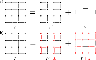
Figure 1: Sketch of plain CPT (a) and conserving CPT (b). Plain CPT: the hopping matrix $T$ is decomposed as $T=T^{\prime}+V$ into the intra-cluster ($T^{\prime}$) and the inter-cluster hopping $V$. The problem defined by $T^{\prime}$ (and the local Hubbard-type interaction) is solved exactly. $V$ is treated by all-order perturbation theory (neglecting vertex corrections), see Eq. (12). Conserving CPT: the same as plain CPT but with “renormalized” intra- ($T^{\prime}-\lambda$) and inter-cluster hopping $V+\lambda$, where the time-dependent renormalization $\lambda$ (indicated in red) is used to enforce conservation laws. Note that $\lambda$ may also comprise the on-site energies.

A closer look reveals that the CPT is not unique since one may consider a different starting point for the all-order perturbation theory in $V$. To this end, consider a starting point with a renormalized intra-cluster hopping, $T^{\prime}\rightarrow T^{\prime}-\lambda$, resulting in a renormalized cluster Green’s function $G_{T^{\prime}-\lambda,U}$ and self-energy $\Sigma_{T^{\prime}-\lambda,U}$. Correspondingly, also the inter-cluster hopping $V$ must be renormalized as $V\rightarrow V+\lambda$. Summation of the geometrical series yields

$$G^{\mathrm{CPT}}[\lambda]=\frac{1}{G_{T^{\prime}-\lambda,U}^{-1}-(V+\lambda)}=\frac{1}{G_{T,0}^{-1}-\Sigma_{T^{\prime}-\lambda,U}},$$ (14)

where we emphasized the special role of the renormalization parameter $\lambda$ by square brackets. For $U(t)=0$, we have $G^{\text{CPT}}[\lambda]=G_{T,0}$ for any $\lambda$. For an interacting system, however, the choice for $\lambda$ is crucial, i.e., the resulting CPT Green’s function does depend on the starting point of the all-order perturbation theory in the inter-cluster hopping.

This ambiguity in the definition of the CPT seems to be problematic on first sight, yet it can be turned into an advantage by interpreting the renormalization $\lambda$ as an optimization parameter. This has been worked out systematically in the context of the (nonequilibrium) self-energy functional theory (SFT), Hofmann et al. (2013); Hofmann et al. (2016a, b); Hofmann and Potthoff (2016) where the optimal $\lambda$ is derived from a variational principle based on the self-energy. Here, we will take a different route and use the freedom in $\lambda$ to enforce the local constraints on spin-dependent particle and doublon density. Physically, the parameter set $\lambda$ must be interpreted as a nonlocal mean-field and the resulting conserving CPT as a cluster mean-field theory.

III.2 Formulation of the conservation laws as local constraints

While conservation laws like particle-number or energy conservation are naturally fulfilled if one is able to treat a physical problem exactly, this is not necessarily the case when working with approximate methods. For Green’s-function-based methods it was shown by Baym and Kadanoff Baym and Kadanoff (1961); Baym (1962) that respecting certain symmetry relations for the two-particle Green’s function is sufficient to ensure that an approximation is conserving.

Here, we build on an equivalent formulation of the macroscopic conservation laws for the particle number, spin and energy and reformulate them as local constraints for the spin-dependent particle density and the doublon density, respectively. This is in the spirit of expressing conservation laws of a classical field theory as continuity equations and follows the work of Baym and Kadanoff. Baym and Kadanoff (1961); Baym (1962) One should note, however, that in our case the local constraints cannot be written in the standard form of continuity equations, as here we aim at an approach for a discrete lattice model.

To discuss the local constraints, we first consider the exact time evolution of a system described by the Hubbard Hamiltonian $H_{T,U}(t)$. We write $G\equiv G_{T,U}$, $G^{(2l)}\equiv G^{(2l)}_{T,U}$ and $G^{(2r)}\equiv G^{(2r)}_{T,U}$ in this subsection to keep the notation simple. The exact time evolution of the system will preserve the total particle number and the $z$-component of the total spin as can be expressed by the following local constraint for the spin-dependent density:

$$0 =\partial_{t}\langle{\hat{n}_{i\sigma}(t)}\rangle_{H_{T,U}}-[G\circ T-T\circ G]_{ii\sigma}(t,t^{+}),$$

$$\Leftrightarrow\quad F_{i\sigma}(t) \equiv G^{(2l)}_{ii\sigma}(t,t^{+})-G^{(2r)}_{ii\sigma}(t,t^{+})=0\;,$$ (15)

as can be verified directly using Eq. (11).

The first line of Eq. (15) constitutes the discrete-lattice analog of the continuity equation for the spin-dependent particle density. Opposed to a continuum theory, however, the divergence of the spin-dependent particle-current density is replaced by the commutator. The second line of Eq. (15) is an equivalent formulation of the same constraint as has originally been mentioned by Baym and Kadanoff. Baym and Kadanoff (1961); Baym (1962)

Next, we consider the following local constraint for the doublon density [cf. Eq. (11)]:

$$C_{i\sigma}(t)\equiv\,\, i\partial_{t}\left[G^{(2l)}_{ii\sigma}(t,t^{+})+G^{(2r)}_{ii\sigma}(t,t^{+})\right]$$ (16)

$$-2\sum_{j\sigma}\left[T_{ij\sigma}(t)G^{(2r)}_{ji\sigma}(t,t^{+})-G^{(2l)}_{ij\sigma}(t,t^{+})T_{ji\sigma}(t)\right]=0.$$

In the exact theory, this constraint together with the above constraint $F_{i\sigma}(t)=0$ expresses the necessity that the doublon density can be derived consistently from either $G^{(2l)}$ or $G^{(2r)}$ and for each spin component $\sigma$ in Eq. (11).

More important, in case of a time-independent Hamiltonian, i.e., if $H_{T,U}(t)=\mathrm{const.}$ for $t>t_{0}$, Eq.  (16) implies total-energy conservation. This is explicitly shown in the Appendix A where, for completeness, also a formal derivation of Eq. (16) is carried out.

While in the exact theory the equations $F_{i\sigma}(t)=0$ and $C_{i\sigma}(t)=0$ must hold necessarily, this is no longer guaranteed in an approximate approach. In particular, the equations are usually violated within the conventional CPT.

The important point is that via Eqs. (7) and (9) both, $G^{(2l)}$ and $G^{(2r)}$, can be expressed in terms of the single-particle Green’s function and the self-energy and thus both equations $F_{i\sigma}(t)=0$ and $C_{i\sigma}(t)=0$ can be expressed in terms of the central quantities of the CPT. Furthermore, as is shown below, they can be incorporated in the Markovian time-propagation scheme based on the Hamiltonian formulation of the CPT. The latter is essential for the numerical treatment.

Our main idea is thus to enforce the local constraints $F_{i\sigma}(t)=0$ and $C_{i\sigma}(t)=0$ within the context of the CPT by exploiting the above-discussed freedom in the choice of the CPT starting point, i.e., by choosing an appropriate renormalization $\lambda=\lambda^{\mathrm{opt}}$. If $\lambda^{\mathrm{opt}}$ can be found, this automatically ensures the conservation of particle number, spin and energy.

IV Hamiltonian-based formulation

In the last section we have introduced the CPT in its usual form, i.e., based on the self-energy $\Sigma_{T^{\prime}-\lambda,U}$ of the reference system and Dyson’s equation. A major drawback of this approach is its limitation for the maximum propagation time that can be reached in a practical numerical calculation. This is due to the fact that the CPT Green’s function and the self-energy of the reference system are nonlocal in time through their dependence on two contour times. The necessary storage for these quantities scales quadratically with the maximum propagation time, the effort for solving Dyson’s equation scales cubically. This intrinsic limitation can be overcome if a so-called Lehmann representation of the self-energy is available. This allows us to solve the Dyson equation by means of a Markovian propagation scheme which permits to reach much longer time scales. Balzer and Eckstein (2014); Gramsch and Potthoff (2015) In the following, we consider this Lehmann representation of the self-energy as given. Its existence for an arbitrary, fermionic lattice system out of equilibrium has been shown in Ref. Gramsch and Potthoff, 2015 where also a constructive numerical scheme has been presented. It can be used in case of small clusters accessible to exact-diagonalization techniques. In the following we briefly recall the main results and then discuss the application to conservation laws and the respective local constraints.

IV.1 Convolution-free definition of $G^{(2l)}$ and $G^{(2r)}$

The nonequilibrium self-energy $\Sigma\equiv\Sigma_{T,U}$ of any lattice-fermion model has a unique Lehmann representation: Gramsch and Potthoff (2015)

$$\Sigma_{ij\sigma}(t,t^{\prime}) =\delta_{C}(t,t^{\prime})\Sigma^{\mathrm{HF}}_{ij\sigma}(t)+\sum_{s\sigma}h_{is\sigma}(t)g(h_{ss\sigma};t,t^{\prime})h^{*}_{js\sigma}(t^{\prime})\>.$$ (17)

Here, $\Sigma_{ij\sigma}^{\mathrm{HF}}(t)$ is the time-local Hartree-Fock term. The second term has a hybridization-function-like structure Gramsch et al. (2013); Balzer and Eckstein (2014) where $h_{is\sigma}(t)$ denotes the hopping between a physical site $i$ and an additional virtual site labeled by the index $s$. The time-independent on-site energy of the virtual site is given by $h_{ss}$. Furthermore, $g(\epsilon;t,t^{\prime})$ is the noninteracting Green’s function of an isolated one-particle mode ($h_{\mathrm{mode}}=\epsilon c^{\dagger}c$) with excitation energy $\epsilon$:

$$g(\epsilon;t,t^{\prime})=i[f(\epsilon)-\Theta_{C}(t,t^{\prime})]e^{-i\epsilon(t-t^{\prime})}.$$ (18)

Here, $f(\epsilon)=(e^{\beta\epsilon}+1)^{-1}$ denotes the Fermi-function, and $\Theta_{C}(t,t^{\prime})$ refers to the contour variant of the Heaviside step function, i.e., $\Theta_{C}(t,t^{\prime})=1$ for $t\geq_{C}t^{\prime}$, and $\Theta_{C}(t,t^{\prime})=0$ otherwise.

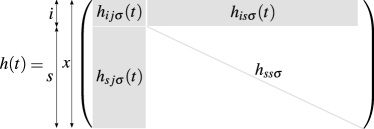
Figure 2: The effective, one-particle Hamiltonian, (21), has three distinct kind of elements. The hybridization elements $h_{is\sigma}(t)=h^{*}_{si\sigma}(t)$, the elements $h_{ij\sigma}(t)$ of the physical sector and the time-independent elements $h_{ss^{\prime}\sigma}\propto\delta_{ss^{\prime}}$ of the virtual sector.

The hybridization-function-like structure is the immediate and important advantage of the Lehmann representation. It allows to write down an effective, noninteracting model specified by the Hamiltonian

$$H^{\mathrm{eff}}(t)=\sum_{ij\sigma} \left(T_{ij\sigma}(t)-\delta_{ij}\mu+\Sigma^{\mathrm{HF}}_{ij\sigma}(t)\right)c^{\dagger}_{i\sigma}c_{j\sigma}$$ (19)

$$+ \sum_{is\sigma}\left(h_{is\sigma}(t)c^{\dagger}_{i\sigma}c_{s\sigma}+\mathrm{h.c.}\right)+\sum_{s}h_{ss\sigma}c^{\dagger}_{s\sigma}c_{s\sigma},$$

which reproduces the one-particle Green’s function $G\equiv G_{T,U}$ exactly when evaluated at the physical sites $i,j$. We emphasize that $H^{\mathrm{eff}}(t)$ includes all correlation effects through the hybridization strengths $h_{is\sigma}(t)$ and on-site energies $h_{ss\sigma}$ of the virtual sites. Furthermore, the previously mentioned interpretation of the $s$-degrees of freedom as additional virtual sites becomes obvious in Eq. (19).

For a given arbitrary self-energy one would typically have to consider a continuum of virtual sites. Here, however, the situation is much simpler since $\Sigma_{ij\sigma}(t,t^{\prime})$ is the CPT self-energy, i.e., the self-energy of our reference model consisting of a system of decoupled clusters. In this case the total number of physical and of necessary virtual sites equals the number of single-particle excitations with nonzero weight. Gramsch and Potthoff (2015) As the latter grows exponentially with the size of the individual cluster, the exact mapping and the exact numerical construction of the effective Hamiltonian is limited to clusters small enough to allow for an exact numerical diagonalization. The computation of the parameters of the effective Hamiltonian (19) is nontrivial but straightforward and numerically completely stable. Details are described in Ref. Gramsch and Potthoff, 2015.

For clarity, we use the following convention throughout the paper:

physical sites: $$~{}~{}i,j,k,l,\qquad\qquad$$ (20)

virtual sites: $$~{}~{}s,s^{\prime},$$

physical or virtual sites: $$~{}~{}x,y.$$

Defining $h_{ij\sigma}(t)\equiv T_{ij\sigma}(t)-\delta_{ij}\mu+\Sigma^{\mathrm{HF}}_{ij\sigma}(t)$, the effective Hamiltonian can be written as (cf. Fig. 2)

$$H^{\mathrm{eff}}(t)=\sum_{xy\sigma}h_{xy\sigma}(t)c^{\dagger}_{x\sigma}c_{y\sigma}.$$ (21)

The corresponding Green’s function is given on the physical but also on the virtual sites,

$$G_{xy\sigma}(t,t^{\prime})=-i\langle{\mathcal{T}_{C}\,\hat{c}_{x\sigma}(t)\hat{c}^{\dagger}_{y\sigma}(t^{\prime})}\rangle_{H^{\mathrm{eff}}},$$ (22)

so that the original, physical Green’s function $G_{ij\sigma}(t,t^{\prime})$ is obtained if we restrict $x,y$ to physical sites only, i.e., $(x,y)=(i,j)$.

Many-particle correlation functions, e.g., spin-spin correlations, are in general not accessible from the effective Hamiltonian. There is, however, one important exception. Namely, the two-particle Green’s functions $G^{(2l)}$ and $G^{(2r)}$ can be expressed as contour convolutions of the system’s self-energy with the Green’s function, cf. Eqs. (7) and (9). In the Hamiltonian-based formalism this convolution is greatly simplified and becomes a straightforward matrix multiplication. By comparing Dyson’s equation (3) with the equation of motion that follows from Eq. (22), one readily finds the identity

$$[\Sigma\circ G]_{ij\sigma}(t,t^{\prime})= \sum_{l}\left[h_{il\sigma}(t)-T_{il\sigma}(t)+\delta_{il}\mu\right]G_{lj\sigma}(t,t^{\prime})$$

$$+\sum_{s}h_{is\sigma}(t)G_{sj\sigma}(t,t^{\prime}).$$ (23)

An analogous relation can be derived for $G\circ\Sigma$.

The result can be written in a more compact form by defining a new quantity $\eta_{xy\sigma}(t)$ via

$$h_{ij\sigma}(t) =U(t)\eta_{ij\sigma}(t)+T_{ij\sigma}(t)-\delta_{ij}\mu,$$ (24)

$$h_{is\sigma}(t) =U(t)\eta_{is\sigma}(t),$$

and $\eta_{ss^{\prime}\sigma}(t)\equiv 0$. This is consistent with the alternative definition given in Appendix B which also holds for $U(t)=0$. In the physical sector it implies

$$\eta_{ij\sigma}(t)=\delta_{ij}\langle{\hat{n}_{i\bar{\sigma}}(t)}\rangle_{H_{T,U}},$$ (25)

as follows from $U(t)\eta_{ij\sigma}(t)=\Sigma^{\text{HF}}_{ij\sigma}(t)$ [cf. Eqs. (19), (21) and (24)]. With this definition for $\eta$ and with the relations $\Sigma\circ G=-iU\circ G^{(2l)}$ and $G\circ\Sigma=-iG^{(2r)}\circ U$ we get

$$G^{(2l)}_{ij\sigma}(t,t^{\prime}) =i\sum_{x}\eta_{ix\sigma}(t)G_{xj\sigma}(t,t^{\prime}),$$ (26)

$$G^{(2r)}_{ij\sigma}(t,t^{\prime}) =i\sum_{x}G_{ix\sigma}(t,t^{\prime})\eta^{*}_{ix\sigma}(t^{\prime}),$$ (27)

Recall at this point that quantities like $h(t)=h_{T,U}(t)$ or $\eta(t)=\eta_{T,U}(t)$ (as well as $H^{\mathrm{eff}}(t)$, $G^{(2l)}$, etc.) are functionals of $T$ and $U$.

IV.2 Hamiltonian-based formulation of the CPT

Let us now discuss how the CPT Green’s function can be obtained from an effective one-particle Hamiltonian and how to set up a Markovian time-propagation scheme. Gramsch and Potthoff (2015) As discussed in Sec. III.1, we have $T=T^{\prime}+V$ where $T^{\prime}-\lambda$ is the renormalized intra-cluster and $V+\lambda$ the renormalized inter-cluster hopping. For each set of parameters $\lambda$, an effective one-particle CPT Hamiltonian can be defined by adding the inter-cluster hopping to the effective Hamiltonian (19) of the reference system:

$$H^{\text{CPT}}[\lambda](t) =H^{\mathrm{eff}}_{T^{\prime}-\lambda,U}(t)+\sum_{ij\sigma}[V_{ij\sigma}(t)+\lambda_{ij\sigma}(t)]c^{\dagger}_{i\sigma}c_{j\sigma}$$

$$\equiv\sum_{xy\sigma}h^{\text{CPT}}_{xy\sigma}(t)c^{\dagger}_{x\sigma}c_{y\sigma}.$$ (28)

The CPT Green’s function, as computed from $H^{\text{CPT}}[\lambda](t)$,

$$G^{\text{CPT}}[\lambda]_{xy\sigma}(t,t^{\prime})=-i\langle{\mathcal{T}_{C}\hat{c}_{x\sigma}(t)\hat{c}^{\dagger}_{y\sigma}(t^{\prime})}\rangle_{H^{\text{CPT}}[\lambda]}$$ (29)

then coincides with the original definition in Eq. (14) if only the physical sector is considered, i.e., $(x,y)=(i,j)$. This can be verified easily by integrating out the virtual, $s$ degrees of freedom from $H^{\mathrm{CPT}}$. Eq. (IV.2) reflects the freedom we have in the CPT construction as the $\lambda$-terms cancel in the physical sector. $\lambda$ only enters implicitly through the hybridization strengths $h^{\prime}_{is\sigma}(t)$, through the on-site energies $h^{\prime}_{ss\sigma}$ (where $h^{\prime}\equiv h_{T^{\prime}-\lambda,U}$) and through the Hartree-Fock term $\Sigma_{T^{\prime}-\lambda,U}^{\mathrm{HF}}$ of the reference system’s Hamiltonian $H_{T^{\prime}-\lambda,U}$.

For each set of parameters $\lambda$, the two-particle correlation function $G^{(2l)}$ is approximated within the context of the CPT as

$$G^{(2l)}[\lambda]_{ij\sigma}(t,t^{\prime}) =i\sum_{x}\eta^{\prime}[\lambda]_{ix\sigma}(t)G^{\text{CPT}}[\lambda]_{xj\sigma}(t,t^{\prime}),$$ (30)

where we have defined

$$\eta^{\prime}[\lambda]\equiv\eta_{T^{\prime}-\lambda,U}.$$ (31)

Eq. (30) corresponds to the exact expression given by Eq. (26). $G^{(2r)}[\lambda]$ is defined analogously, and thus the symmetry relation

$$G^{(2r)}[\lambda]_{ji\sigma}(t,t^{+})=\left[G^{(2l)}[\lambda]_{ij\sigma}(t,t^{+})\right]^{*}$$ (32)

is ensured within the CPT independently of $\lambda$. Note that this symmetry is not sufficient to allow for an unambiguous definition of the doublon density based on $G^{(2l)}$ and $G^{(2r)}$ [cf. Eq. (11)]. Instead, it requires both constraints to be respected as discussed in Sec. III.2. In case of an arbitrary, non-conserving set of parameters $\lambda$ this ambiguity needs to be circumvented by defining the doublon density as an average

$$d_{i}[\lambda](t)=-\frac{1}{4}\sum_{\sigma}\left[G^{(2l)}[\lambda]_{ii\sigma}(t,t^{+})+G^{(2l)}[\lambda]_{ii\sigma}(t,t^{+})\right].$$ (33)

For $\lambda=\lambda^{\text{opt}}$, however, we have

$$d_{i}[\lambda^{\text{opt}}](t)=-G^{(2l)}[\lambda^{\text{opt}}]_{ii\sigma}(t,t^{+})=-G^{(2r)}[\lambda^{\text{opt}}]_{ii\sigma^{\prime}}(t,t^{+}).$$ (34)

The final forms of the conditional equations for $\lambda^{\text{opt}}$ are obtained by replacing $G^{(2r)}$ and $G^{(2l)}$ by their CPT approximations $G^{(2l)}[\lambda]$ and $G^{(2r)}[\lambda]$ in the expressions for $F$ and $C$ given by Eqs. (15) and (16):

$$F[\lambda^{\text{opt}}]_{i\sigma}(t)\stackrel{{\scriptstyle!}}{{=}}0,\quad C[\lambda^{\text{opt}}]_{i\sigma}(t)\stackrel{{\scriptstyle!}}{{=}}0.$$ (35)

We note that the number of free parameters $\lambda$ must be chosen to match the number of linear independent constraints defined by Eq. (35) to ensure the existence of a unique solution $\lambda^{\text{opt}}$.

V Solving the self-consistency equations

Having formulated the self-consistency conditions (35), it remains to explicitly solve these equations for $\lambda^{\text{opt}}$. An important simplification arises from the fact that the CPT is by construction a fully causal theory, i.e., the time-local elements $G^{\text{CPT}}(t,t^{+})$ of the CPT Green’s function at time $t$, for example, only depend on quantities at earlier times. The same holds for $G^{(2l)}(t,t^{+})$ and for $h^{\text{CPT}}_{xy\sigma}(t)$. This allows us to construct a strategy for the solution of Eq. (35) in the form of a time-propagation algorithm. Let us therefore assume that $\lambda^{\text{opt}}$ is known for all time points on a discrete time grid and that only the parameters $\lambda^{\text{opt}}(t)$ at the latest point of time $t$ are unknown.

Therewith, the actual task is to solve Eq. (35) for $\lambda^{\text{opt}}(t)$ only at the given latest point of time $t$. To this end we have to analyze at time $t$ the $\lambda(t)$ dependence of the relevant quantities, i.e., of $G^{(2l)}(t,t^{+})$ and $G^{(2r)}(t,t^{+})$, see Eqs. (15) and (16). First of all, the dependence of $G^{(2l)}(t,t^{+})$ (and $G^{(2r)}(t,t^{+})$) on $\lambda(t)$ at time $t$ is due to the CPT Hamiltonian $h^{\text{CPT}}_{xy\sigma}(t)$ [see Eq. (IV.2) and see Eqs. (29) and (30)]. The $\lambda(t)$-dependence of the latter is exclusively due to the time-evolution operator $\mathcal{U}^{\prime}[\lambda]\equiv\mathcal{U}_{T^{\prime}-\lambda,U}$ of the reference system. The detailed construction of $h^{\text{CPT}}_{xy\sigma}(t)$ is not important here, and we refer to Ref. Gramsch and Potthoff, 2015 for a comprehensive discussion. Finally, the functional dependence of $U^{\prime}[\lambda](t,0)$ on $\lambda$ is through an integration over all times between $0$ and $t$. With this information at hand, we are in fact able to characterize the dependence on $\lambda(t)$ at time $t$ of the quantities $G^{(2l)}(t,t^{+})$ and $G^{(2r)}(t,t^{+})$ which enter the local constraints (35) that serve to enforce the conservation laws.

The most important point for the following discussion is the fact that, in the limit of vanishing time step $\Delta t\to 0$, the parameter set $\lambda(t)$ at the latest point of time enters basically all central quantities as a null set only: Consider, for example, $G^{(2l)}(t,t^{+})$. Its first-order response due to a variation of $\lambda(t)$ at time $t$ vanishes (as shown below). On the one hand, this missing sensitivity implies a complication of the theory since one has to account for this mathematical property explicitly when setting up a numerical implementation. On the other hand, once one has recognized the property, it actually helps to the solve Eqs. (35). Consider a given arbitrary causal functional $M[\lambda](t)$. The main trick is to enhance the sensitivity of $M[\lambda](t)$ to variations of $\lambda(t)$ at time $t$ by taking its time derivative. Typically, if the first-order response of $M[\lambda](t)$ vanishes, $\partial_{t}M[\lambda](t)$ is a linear function of $\lambda(t)$ at time $t$. Clearly, this is the key to solve an equation like $M[\lambda](t)=0$ for $\lambda^{\text{opt}}(t)$.

In the following subsections V.1 – V.4 the above-sketched ideas are worked out on a more technical level. Finally, the section V.5 addresses the initial state at time $t=0$.

V.1 Time-local variations

Assume that we have found the optimal renormalization $\lambda^{\text{opt}}(t)$ for $t\leq t_{n}\equiv n\,\Delta t$. We introduce a variation $\delta_{\mathrm{loc}}^{n}$ which affects the current (the $n$-th) time step only:

$$\delta_{\mathrm{loc}}^{n}\lambda_{ij\sigma}(t)=\delta\lambda_{ij\sigma}(t)\Theta^{n}_{\mathrm{loc}}(t),\quad\Theta^{n}_{\mathrm{loc}}(t)=\left\{\begin{aligned} 1\,\,\,\,&\text{if}\,\,\,\,{t\in\left[t_{n},t_{n+1}\right]},\\ 0\,\,\,\,&\text{else}.\end{aligned}\right.$$ (36)

For simplicity, we require the variations to be symmetric, i.e., $\delta\lambda_{ij\sigma}(t)=\delta\lambda_{ji\sigma}(t)$. This implies a restriction to symmetric solutions $\lambda^{\text{opt}}$. Consider now an arbitrary, causal functional $M[\lambda](t)$, i.e., a functional that at time $t$ only depends on $\lambda(t^{\prime})$ with $t^{\prime}\leq t$. For such an object, the variational operator $\delta_{\mathrm{loc}}^{n}$ is related to the conventional functional derivative through

$$\delta_{\mathrm{loc}}^{n}M[\lambda](t) =\sum_{\sigma}\sum_{i\geq j}\int_{t_{n}}^{t}\mathrm{d}t^{\prime}\frac{\delta M[\lambda](t)}{\delta\lambda_{ij\sigma}(t^{\prime})}\delta\lambda_{ij\sigma}(t^{\prime}),$$ (37)

where the restriction $i\geq j$ is necessary because of the symmetry requirement $\lambda_{ij\sigma}=\lambda_{ji\sigma}$.

We now take the combined limit $n\rightarrow\infty,\,\Delta t\rightarrow 0$ such that we always have $t\in[t_{n},t_{n+1}]$ to define the time-local variation $\delta_{\mathrm{loc}}$ in the continuum limit

$$\delta_{\mathrm{loc}}M[\lambda](t) =\lim_{\begin{subarray}{c}\Delta t\rightarrow 0\\ n\rightarrow\infty\end{subarray}}\delta_{\mathrm{loc}}^{n}M[\lambda](t),$$ (38)

with the corresponding variational quotient

$$\frac{\delta_{\mathrm{loc}}M[\lambda](t)}{\delta_{\mathrm{loc}}\lambda_{ij\sigma}(t)}\equiv\lim_{\begin{subarray}{c}\Delta t\rightarrow 0\\ n\rightarrow\infty\end{subarray}}\int_{t_{n}}^{t}\mathrm{d}t^{\prime}\frac{\delta M[\lambda](t)}{\delta\lambda_{ij\sigma}(t^{\prime})}.$$ (39)

This variational quotient describes the linear response of $M[\lambda](t)$ when varying the parameters at the latest time step:

$$\delta_{\mathrm{loc}}M[\lambda](t)=\sum_{\sigma}\sum_{i\geq j}\frac{\delta_{\mathrm{loc}}M[\lambda](t)}{\delta_{\mathrm{loc}}\lambda_{ij\sigma}(t)}\delta\lambda_{ij\sigma}(t).$$ (40)

V.2 Integrated quantities in $\lambda$

With the appropriate variation for our purposes at hand, we can study the effect of the variation on the main quantities within the CPT framework. We first consider the time-evolution operator (“propagator”) of the reference system $\mathcal{U}^{\prime}[\lambda]\equiv\mathcal{U}_{T^{\prime}-\lambda,U}$. It is instructive to study the effect of the operator $\delta_{\mathrm{loc}}^{n}$ first, i.e., the effect of a time-local variation with finite time step $\Delta t$. Keeping only terms of the order $O(\Delta t)$ one finds

$$\delta_{\mathrm{loc}}^{n}\mathcal{U}^{\prime}[\lambda](t,0) =-i\left[\sum_{ij\sigma}\int_{t_{n}}^{t}\delta\lambda_{ij\sigma}(t^{\prime})\hat{c}^{\dagger}_{i\sigma}\hat{c}_{j\sigma}\mathrm{d}t^{\prime}\right]\mathcal{U}^{\prime}[\lambda](t_{n},0)$$

$$\phantom{=}\,\,+O(\Delta t^{2}).$$ (41)

In lowest order we thus have $\delta_{\mathrm{loc}}^{n}\mathcal{U}_{T^{\prime}-\lambda,U}(t,0)\propto\Delta t\,\delta\lambda(t)$. This means that the linear response vanishes identically in the limit $\Delta t\rightarrow 0$. This property originates from the fact that $\lambda(t)$ is integrated over time within the propagator $\mathcal{U}_{T^{\prime}-\lambda,U}(t,0)$, and that the contribution of a single time step, $t\in[t_{n},t_{n+1}]$, to this integral is of zero measure in the limit $\Delta t\rightarrow 0$.

A finite time-local variation is obtained for the first time derivative of the propagator rather than for the propagator itself. Namely, the corresponding time-local variational quotient remains non-zero in the continuum limit:

$$\frac{\delta_{\mathrm{loc}}[i\partial_{t}\mathcal{U}^{\prime}[\lambda](t,0)]}{\delta_{\mathrm{loc}}\lambda_{ij\sigma}(t)}=-\bigl{[}c^{\dagger}_{j\sigma}c_{i\sigma}+c^{\dagger}_{i\sigma}c_{j\sigma}-\delta_{ij}c^{\dagger}_{i\sigma}c_{i\sigma}\bigr{]}\mathcal{U}^{\prime}[\lambda](t,0).$$ (42)

Multiplying this equation with $\lambda_{ij\sigma}(t)$, summing over $i,j,\sigma$ and comparing with the standard equation of motion $i\partial_{t}\mathcal{U}^{\prime}[\lambda](t,0)=H_{T^{\prime}-\lambda,U}(t)\mathcal{U}^{\prime}[\lambda](t,0)$, shows that the time derivative of the propagator is of the general form

$$i\partial_{t}\mathcal{U}^{\prime}[\lambda](t,0)=\sum_{\sigma}\sum_{i\geq j}\frac{\delta_{\mathrm{loc}}[i\partial_{t}\mathcal{U}^{\prime}[\lambda](t,0)]}{\delta_{\mathrm{loc}}\lambda_{ij\sigma}(t)}\lambda_{ij\sigma}(t)+\xi_{\mathcal{U}^{\prime}}[\lambda](t),$$ (43)

where $\xi_{\mathcal{U}^{\prime}}[\lambda](t)=H_{T^{\prime},U}(t)\mathcal{U}^{\prime}[\lambda](t,0)$. Note that the dependence on $\lambda_{ij\sigma}(t)$ at time $t$ is strictly linear in the limit $\Delta t\to 0$.

With this definition and with Eq. (42), it is obvious that the variational derivative and $\xi_{\mathcal{U}^{\prime}}[\lambda](t)$ on the right-hand side of Eq. (43) depend on $\lambda(t)$ only through an integration over time within the propagator $\mathcal{U}^{\prime}[\lambda](t,0)$. We will call such quantities integrated quantities in $\lambda$. Integrated quantities in $\lambda$ inherit an important property from the cluster propagator $\mathcal{U}^{\prime}[\lambda]$, see Eq. (41): Their time-local variation vanishes in the limit $\Delta t\rightarrow 0$.

Furthermore, the time derivative of any quantity $M[\lambda]$ that is integrated in $\lambda$, i.e., the time derivative of a functional of the form $M[\lambda](t)=M(\mathcal{U}^{\prime}[\lambda](t,0))$, can be brought into a form analogous to Eq. (43). This follows immediately from the chain rule in calculus as $i\partial_{t}M[\lambda](t)=\frac{i\partial M(\mathcal{U}^{\prime})}{\partial\mathcal{U}^{\prime}}\frac{\partial\mathcal{U}^{\prime}[\lambda](t,0)}{\partial t}$. Explicitly this result reads

$$i\partial_{t}M[\lambda](t)=\sum_{\sigma}\sum_{i\geq j}\frac{\delta_{\mathrm{loc}}[i\partial_{t}M[\lambda](t)]}{\delta_{\mathrm{loc}}\lambda_{ij\sigma}(t)}\lambda_{ij\sigma}(t)+\xi_{M}[\lambda](t),$$ (44)

where $\frac{\delta_{\mathrm{loc}}[i\partial_{t}M[\lambda](t)]}{\delta_{\mathrm{loc}}\lambda_{ij\sigma}(t)}$ and $\xi_{M}[\lambda]$ are again integrated quantities in $\lambda$. We furthermore conclude that a time-local variation of the time derivative of an integrated quantity in $\lambda$ is non-zero in general.

The main idea in the following is to combine the conditional equations (35) into a single equation $\Gamma[\lambda^{\text{opt}}](t)\stackrel{{\scriptstyle!}}{{=}}0$ such that $\Gamma[\lambda]$ is of the form $\Gamma[\lambda](t)=J[\lambda](t)\lambda(t)+\xi_{\Gamma}[\lambda](t)$ where $J[\lambda]$ and $\xi_{\Gamma}[\lambda]$ are integrated quantities in $\lambda$. This is formally easily solved for $\lambda^{\text{opt}}(t)$ by matrix inversion and allows to derive an efficient propagation scheme for numerical purposes.

V.3 $\lambda$-dependence of $G^{(2l)}$ and $G^{(2r)}$

The main building blocks of the local constraints on the spin-dependent density, Eq.  (15), and the doublon density, Eq. (16), are given by the two-particle correlation functions $G^{(2l)}$ and $G^{(2r)}$. Within the CPT approximation they are defined through Eq.  (30). We therefore have to understand the $\lambda$ dependence of $\eta^{\prime}[\lambda]\equiv\eta_{T^{\prime}-\lambda,U}$ and $G^{\text{CPT}}[\lambda]$.

One can easily see that $\eta^{\prime}[\lambda]$ is an integrated quantity in $\lambda$. Consider, for example, the physical sector. From Eq. (25) we have $\eta^{\prime}_{ij\sigma}[\lambda](t)=\delta_{ij}\langle{\hat{n}_{i\bar{\sigma}}(t)}\rangle_{H_{T^{\prime}-\lambda,U}}$. The only $\lambda$-dependence of this expression indeed stems from the propagator $\mathcal{U}^{\prime}[\lambda]$. To obtain a non-vanishing time-local variation we thus have to consider the first derivative with respect to time. This is worked out in Appendix C:

$$\delta_{\mathrm{loc}}[i\partial_{t}\eta^{\prime}_{ij\sigma}(t)] =\eta^{\prime}_{ii\sigma}(t)\delta\lambda_{ij\sigma}(t)-\sum_{l\sigma^{\prime}}[\delta\lambda_{il\sigma^{\prime}}(t)]\gamma^{l\sigma^{\prime}}_{ij\sigma}(t),$$

$$\delta_{\mathrm{loc}}[i\partial_{t}\eta^{\prime}_{is\sigma}(t)] =-\sum_{l\sigma^{\prime}}[\delta\lambda_{il\sigma^{\prime}}(t)]\gamma^{l\sigma^{\prime}}_{is\sigma}(t),$$ (45)

where the newly introduced tensor $\gamma[\lambda]^{l\sigma^{\prime}}_{is\sigma}(t)$ is cluster-diagonal, i.e., $\gamma[\lambda]^{l\sigma^{\prime}}_{is\sigma}(t)\neq 0$ if and only if $i$ and $l$ refer to lattice sites within the same cluster. It furthermore follows that $i\partial_{t}\eta^{\prime}[\lambda](t)$ can be brought into the form specified by Eq. (44), where the variational derivative $\frac{\delta_{\mathrm{loc}}[i\partial_{t}\eta^{\prime}[\lambda]_{ix\sigma}(t)]}{\delta\lambda_{jl\sigma}(t)}$, as given by Eq. (45), and $\xi_{\eta^{\prime}}[\lambda]_{ix\sigma}(t)$ are integrated quantities in $\lambda$. An explicit expression for the latter is not needed for our purposes.

Let us now take a look at the CPT Green’s function. It depends on $\lambda$ through the Hamiltonian $H^{\mathrm{CPT}}[\lambda]$, which in turn depends on $\lambda$ through the hybridization strengths $h^{\prime}[\lambda]_{is\sigma}(t)=U(t)\eta^{\prime}[\lambda]_{is\sigma}(t)$ and the Hartree-Fock term $\Sigma^{\prime}[\lambda]^{\text{HF}}_{ij\sigma}(t)=U(t)\eta^{\prime}[\lambda]_{ij\sigma}(t)$. The Hamiltonian $H^{\text{CPT}}(t)$ is therefore an integrated quantity in $\lambda$. As the propagator $\mathcal{U}^{\text{CPT}}[\lambda](t,0)=T\mathrm{exp}\left({-i\int_{0}^{t}\mathrm{d}t^{\prime}H^{\text{CPT}}[\lambda](t^{\prime})}\right)$ involves a second integral over time, we conclude that $\delta_{\mathrm{loc}}^{n}G^{\text{CPT}}(t,t^{+})\propto\Delta t^{2}\,\delta\lambda(t)$. In this sense, $G^{\text{CPT}}$ must be seen as an integrated quantity in $\lambda$ of second order. Consequently, the time-local variation of its first derivative with respect to time vanishes:

$$\delta_{\mathrm{loc}}[i\partial_{t}G^{\text{CPT}}[\lambda](t,t^{+})]=0.$$ (46)

We note that the time derivative involves the product of the matrix elements of the CPT Hamiltonian, Eq. (IV.2), with $G^{\text{CPT}}[\lambda](t,t^{+})$, i.e., the product of an integrated quantity in $\lambda$ with an integrated quantity in $\lambda$ of second order, respectively. Obviously, the product scales like an ordinary integrated quantity in $\lambda$ when a time-local variation is applied, i.e., $\delta_{\mathrm{loc}}^{n}h^{\text{CPT}}(t)G^{\text{CPT}}(t,t^{+})\propto\Delta t\delta\lambda(t)$ in lowest order in $\Delta t$.

Concluding, to get a non-vanishing time-local variation, one must consider the first time derivative of the two-particle Green’s functions $G^{(2l)}$ and $G^{(2r)}$. We find

$$\delta_{\mathrm{loc}}\left[i\partial_{t}G^{(2l)}_{ij\sigma}(t,t^{+})\right]=\sum_{x}\left(\delta_{\mathrm{loc}}[i\partial_{t}\eta^{\prime}_{ix\sigma}(t)]\right)G^{\text{CPT}}_{xj\sigma}(t,t^{+})$$ (47)

and an analogous expression for $G^{(2r)}$. Only the $\eta^{\prime}$-term contributes to the variation, cf. Eq. (45), while the variation of the CPT Green’s function vanishes, cf. Eq. (46). We also note that Eq. (45) may be used at this point and that $i\partial_{t}G^{(2l)}(t,t^{+})$ [and analogously $i\partial_{t}G^{(2r)}(t,t^{+})$] is of the form

$$i\partial_{t}G^{(2l)}_{ij\sigma}(t,t^{+})=\sum_{\sigma^{\prime}}\sum_{k\geq l}\frac{\delta_{\mathrm{loc}}G^{(2l)}_{ij\sigma}(t,t^{+})}{\delta_{\mathrm{loc}}\lambda_{kl\sigma^{\prime}}(t)}\lambda_{kl\sigma^{\prime}}(t)+[\xi_{G^{(2l)}}]_{ij\sigma}(t),$$ (48)

where both, the variational derivative $\frac{\delta_{\mathrm{loc}}G^{(2l)}(t,t^{+})}{\delta_{\mathrm{loc}}\lambda(t)}$, as given by Eq. (47), and the quantity $\xi_{G^{(2l)}}(t)$, which is not needed in explicit form for our purposes, scale like integrated quantities in $\lambda$ under time-local variations. This follows from the fact that $i\partial_{t}G^{\text{CPT}}(t,t^{+})$ scales like an integrated quantity in $\lambda$ under time-local variations and the related discussion above.

V.4 $\lambda$-dependence of the local constraints

The local constraint on the spin-dependent density, Eq. (15), is formulated in terms of the difference between $G^{(2l)}$ and $G^{(2r)}$. Therefore its first derivative with respect to time must be considered to obtain a non-vanishing time-local variation:

$$\delta_{\mathrm{loc}}[i\partial_{t}F[\lambda]_{i\sigma}(t)]=\delta_{\mathrm{loc}} \left[i\partial_{t}G^{(2l)}[\lambda]_{ii\sigma}(t,t^{+})\right.$$ (49)

$$\quad\quad\quad\quad\left.-i\partial_{t}G^{(2r)}[\lambda]_{ii\sigma}(t,t^{+})\right],$$

For the time-local variation of the local constraint on the doublon density, Eq. (16), on the other hand, one finds

$$\delta_{\mathrm{loc}}C[\lambda]_{i\sigma}(t)=\delta_{\mathrm{loc}} \left[i\partial_{t}G^{(2l)}[\lambda]_{ii\sigma}(t,t^{+})\right.$$ (50)

$$\quad\quad\quad\quad\left.+i\partial_{t}G^{(2r)}[\lambda]_{ii\sigma}(t,t^{+})\right],$$

since $\delta_{\mathrm{loc}}[T\circ G^{(2r)}-G^{(2l)}\circ T](t,t^{+})=0$, where we made use of the fact that $T=T^{\prime}+V$ is the hopping of the original system and thus independent of $\lambda$.

To treat both constraints in a combined formal frame, we define the functional $\Gamma[\lambda]$:

$$\Gamma[\lambda]_{a}(t)=\left\{\begin{aligned} &i\partial_{t}F[\lambda]_{i\sigma}(t)\quad\text{if}\quad 0\leq a<2L\>,\\ &C[\lambda]_{i\sigma}(t)\quad\text{if}\quad 2L\leq a<4L\>,\end{aligned}\right.$$ (51)

where $L$ is the number of lattice sites. With this, the conditional equation for the optimal renormalization reads $\Gamma[\lambda^{\text{opt}}]\stackrel{{\scriptstyle!}}{{=}}0$. From the previous discussion and Eq. (48) it follows that $\Gamma[\lambda]_{a}(t)$ is of the form

$$\Gamma[\lambda]_{a}(t)=\sum_{b}J[\lambda]_{ab}(t)\lambda_{b}(t)+\xi_{\Gamma}[\lambda]_{a}(t),$$ (52)

where we introduced the super-index $b$ which labels the set of free parameters: $\lambda_{b}=\lambda_{ij\sigma}$, $i\geq j$. Both $J[\lambda]$ and $\xi_{\Gamma}[\lambda]$ scale like integrated quantities in $\lambda$ under time-local variations. The Jacobian matrix $J$ is defined as

$$J[\lambda]_{ab}(t)\equiv\frac{\delta_{\mathrm{loc}}\Gamma_{a}[\lambda](t)}{\delta_{\mathrm{loc}}\lambda_{b}(t)}.$$ (53)

The matrix $J[\lambda](t)$ is quadratic if the number of free parameters $\lambda_{b}$ is chosen such that it equals the number of conditional equations [see Eq. (51)]. Assuming that $J[\lambda](t)$ is regular, one can formally solve the conditional equation for the optimal renormalization:

$$\Gamma[\lambda^{\text{opt}}](t)\stackrel{{\scriptstyle!}}{{=}}0\quad\Leftrightarrow\quad\lambda^{\mathrm{opt}}(t)=-\left[J[\lambda^{\text{opt}}](t)\right]^{-1}\xi_{\Gamma}[\lambda^{\text{opt}}](t)\>,$$ (54)

see Eq. (52). This completes our derivation.

Let us emphasize that the single point $\lambda^{\mathrm{opt}}(t)$ represents a null set with respect to the time-integrations in $J[\lambda^{\text{opt}}](t)$ and $\xi_{\Gamma}[\lambda^{\text{opt}}](t)$. This can be exploited to derive an efficient numerical scheme to obtain $\lambda^{\text{opt}}(t)$ step by step on the time axis as detailed in Appendix D. There we also argue why finding an explicit expression for $\xi_{\Gamma}[\lambda](t)$ can in fact be circumvented. An explicit expression for $J[\lambda](t)$ in terms of known quantities, on the other hand, is available via Eqs. (45), (47), (49) and (50).

V.5 The equilibrium initial state

Initially, at time $t=0$ the system is assumed to be in a thermal state. The CPT approximation for the initial thermal state suffers from the fact that the starting point of the all-order perturbation theory in the inter-cluster hopping is not unique. This is completely analogous to the CPT description of the real-time dynamics. Unlike the real-time dynamics, however, the local constraints cannot be used to fix the renormalization parameters $\lambda_{\mathrm{eq}}\equiv\lambda(0)$ for the initial state, and thus a nontrivial self-consistency condition is not available, unfortunately.

This can be seen as follows: Let us assume that the hopping matrix $T$, and consequently $T^{\prime}$ and $V$, are real and symmetric. Consider $G^{(2l)}$ at times $t=t^{\prime}=0$. Via Eq. (30) this is given as $G^{(2l)}[\lambda]_{ij\sigma}(0,0^{+})=i\sum_{x}\eta^{\prime}[\lambda]_{ix\sigma}(0)G^{\text{CPT}}[\lambda]_{xj\sigma}(0,0^{+})$. In Appendix B it is shown that at time $t=0$ the imaginary part $\mathrm{Im}\,\{\eta^{\prime}[\lambda]_{ix\sigma}(0)\}$ vanishes, independently of $\lambda_{\mathrm{eq}}$. Hence, Eq.  (24) implies that $H^{\text{CPT}}[\lambda](0)$ is real and symmetric, and therefore $G^{\text{CPT}}[\lambda]_{xy\sigma}(0,0^{+})=i\langle{\hat{c}^{\dagger}_{y\sigma}(0)\hat{c}_{x\sigma}(0)}\rangle_{H^{\text{CPT}}[\lambda]}$ is purely imaginary. Consequently, $G^{(2l)}[\lambda](0,0^{+})$ is real. Finally, we conclude with Eq. (32) that

$$G^{(2l)}[\lambda]_{ij\sigma}(0,0^{+})=G^{(2r)}[\lambda]_{ji\sigma}(0,0^{+}).$$ (55)

This directly proves that $F[\lambda]_{i\sigma}(0)=0$, and furthermore

$$C[\lambda]_{i\sigma}(0)=2\sum_{j\sigma}T_{ij\sigma}(0) \left[G^{(2r)}[\lambda]_{ji\sigma}(0,0^{+})\right.$$ (56)

$$\quad\quad\left.-G^{(2l)}[\lambda]_{ij\sigma}(0,0^{+})\right]=0$$

irrespective of $\lambda_{\mathrm{eq}}$, i.e., both constraints hold trivially.

For the concrete numerical calculations we therefore circumvent this issue and consider a noninteracting initial state. In this case the CPT is exact, independent of the choice of $\lambda$. The initial value $\lambda_{\mathrm{eq}}$ is then fixed by requiring $\lambda$ to be continuous so that $\lambda_{\mathrm{eq}}=\lambda(0^{+})$.

VI Numerical results

The conserving CPT has been implemented numerically. First results are discussed for the two-dimensional Hubbard model on an $L=10\times 10$ square lattice with periodic boundary conditions. As these results shall serve as a proof of concept only, we restrict ourselves to the most simple approximation, i.e., to the smallest meaningful cluster as the building block of the reference system, namely a cluster consisting of $2\times 1$ sites. Hence, the entire system is partitioned into $50$ clusters in total, see Fig. 3.

Initially, the system is prepared in its noninteracting ground state at half-filling by choosing $\mu=0$. Note that the CPT description of this initial state is exact (and independent of the renormalization). The hopping of the original system is restricted to nearest neighbors, and we set the nearest-neighbor hopping $T=1$ to fix energy and time units. To drive the system out of equilibrium we consider an interaction quench where the Hubbard-$U$ is suddenly, at time $t=0$, switched on to a finite value $U_{\text{fin}}$:

$$U(t)=\Theta(t)U_{\text{fin}}.$$ (57)

Here, $\Theta(t)$ denotes the Heaviside step function. For times $t>0$ the interaction strength is constant. To maintain particle-hole symmetry and half-filling, the chemical potential is quenched as well, from $\mu=0$ to $\mu=U/2$ in the final state.

Studying the model at the particle-hole symmetric point is convenient since the conservation of the total particle number is trivially respected in this case. Jurgenowski and Potthoff (2013) For a spin-independent parameter quench, as considered here, the CPT also trivially respects the conservation of the total spin. Total-energy conservation, on the other hand, is violated in a conventional CPT approach as has been explicitly demonstrated recently. Gramsch and Potthoff (2015) For the present setup we will therefore employ the nearest-neighbor hopping within the $2\times 1$ reference system to enforce the energy-conservation law. This specifies the time-dependent renormalization parameter $\lambda(t)$ (see Fig. 3).

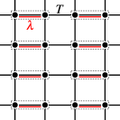
Figure 3: Partitioning of the Hubbard model with nearest-neighbor hopping on the two-dimensional square lattice used for the numerical calculations. Original system: $L=10\times 10$ lattice with periodic boundary conditions. Reference system: $50$ clusters of size $2\times 1$. The figure shows a $4\times 4$ excerpt. Clusters are indicated by dashed rectangles. Nearest-neighbor hopping $T$ and optimization parameter $\lambda(t)$ are indicated by black and red lines. The time-dependent renormalization $\lambda(t)$ is employed to enforce the conservation of energy in the real-time dynamics following an interaction quench.

We note that the computational effort to self-consistently evaluate the presented theory numerically is essentially determined by the underlying solver for the conventional nonequilibrium CPT with little overhead. Here, we use the time-local, Hamiltonian-based solver developed in Ref. Gramsch and Potthoff, 2015 which constructs the effective Hamiltonian of each cluster by exact diagonalization. For the $2\times 1$ reference system under consideration, only two virtual sites are needed for an exact mapping. This gives us four sites per cluster so that the CPT-Hamiltonian comprises $200$ sites in total. Furthermore, regarding computational demands, our approach inherits a constant memory consumption from the CPT solver as well as the linear scaling in the maximum propagation time. In particular, we have used a time step of $\Delta t=0.001$ to propagate the system up to $26,500$ steps up to a maximum propagation time of $t_{\text{max}}=26.5$. For each such time step $t_{n}$, the scheme developed in Appendix D has been employed with $n_{p}=1$, i.e., we have calculated the Taylor coefficients $\lambda_{n,0}$ and $\lambda_{n,1}$.

While the required computational resources are very moderate, accessing longer time scales has turned out to be hindered by mathematical complications. As is obvious from Eq. (54), an inversion of the Jacobian matrix $J(t)$ is necessary to obtain $\lambda^{\text{opt}}(t)$ at each time step. However, with increasing $U_{\text{fin}}$ this matrix exhibits singular points of non-invertibility at earlier and earlier times. In fact, one finds numerically that also the starting point $t=0^{+}$ is singular, namely the Jacobian matrix vanishes: $J(0^{+})=0$. Fortunately, one also has $\xi_{\Gamma}(0^{+})=0$, such that this problem is fixed by applying L’Hôpital’s rule. At time $t=0^{+}$, the defining equation for $\lambda^{\text{opt}}(0^{+})$ becomes

$$\lambda^{\mathrm{opt}}(0^{+})=-\left[\partial_{t}J[\lambda^{\text{opt}}](0^{+})\right]^{-1}[\partial_{t}\xi_{\Gamma}[\lambda^{\text{opt}}](0^{+})].$$ (58)

While this solves the problem at time $t=0^{+}$, finding a systematic and convenient way to propagate beyond the singular points of the Jacobian matrix at finite times remains topic for future investigations.

Apart from this technical problem, the suggested scheme works as expected. Results for the time evolution of the doublon density are shown in Fig. 4. It is evident that the renormalization $\lambda$ has a strong influence on the dynamics and leads to qualitatively different results when comparing the plain unoptimized CPT calculation with the novel conserving CPT. While the dynamics is characterized by ongoing oscillations when using plain CPT, there is a monotonic decay of the doublon density in case of the conserving CPT. The longest maximum propagation time is achieved for the quench $U=0\rightarrow 0.5$. Here, the first singular point of the Jacobian shows up at $t_{\text{max}}\approx 26.5$. On this time scale, the doublon density seems to relax to a stationary state with little to no oscillations.

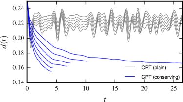
Figure 4: Time evolution of the local doublon density after an interaction quench $U=0\rightarrow U_{\text{fin}}$. Grey lines: plain CPT. Blue lines: conserving CPT. Results for different $U_{\text{fin}}$ ranging from $U_{\text{fin}}=0.5$ (top curve) to $U_{\text{fin}}=1.0$ (bottom) with equidistant steps $\Delta U_{\text{fin}}=0.1$. For the conserving CPT calculations, propagation times are limited by singular Jacobians.

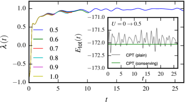
Figure 5: Time evolution of the optimal renormalization parameter $\lambda^{\text{opt}}(t)$ for different $U_{\text{fin}}$ as indicated and corresponding to Fig. 4. Inset: time dependence of the total energy (plain and conserving CPT).

The qualitatively different time dependence of the doublon density reflects the qualitatively different behavior found for the total energy in the plain and the conserving CPT: This is shown in the inset of Fig. 5. For the conserving CPT, the total energy is perfectly conserved within numerical accuracy – by construction of the approach. In the plain CPT calculation, however, the total energy shows unphysical oscillations. Here, maxima and minima of $E_{\rm tot}(t)$ nicely correspond to maxima and minima in the plain-CPT doublon density seen in Fig. 4. It must be concluded that those are artifacts of the plain CPT approach. We also note that small unphysical oscillations of the total energy density $E_{\rm tot}(t)/L$ (with $L=100$) with amplitudes less than $0.01$ lead to much stronger oscillations in the doublon density with amplitudes of about 0.04.

The main part of Fig. 5 displays the results for the time evolution of the renormalization parameter $\lambda(t)$. Its dependence on $U_{\text{fin}}$ turns out to be rather weak on a time scale of a few inverse hoppings. Irrespective to the final interaction strength $U_{\rm fin}$, the initial equilibrium value is found as $\lambda_{\mathrm{eq}}\approx-0.86$. For $t>0$ and for all $U_{\rm fin}$, the renormalization parameter rapidly increases to $\lambda\approx 0.6$ within a very short time $t\approx 0.7$. This corresponds to the rapid initial drop of the doublon density (cf. Fig. 4). Results for longer times are again only available for the quench $U=0\rightarrow 0.5$. On the time scale up to $t_{\rm max}\approx 26.5$, we observe a subsequent slow relaxation of $\lambda(t)$ toward an average final value $\lambda_{\infty}\approx 1.0$ with small superimposed oscillations. It seems reasonable to assume that a similar behavior would also be found for the other quenches, given that the short-time dynamics is very similar for the different $U_{\rm fin}$.

One should note that $\lambda_{\infty}=1$ amounts $T^{\prime}-\lambda_{\infty}=0$, i.e., a vanishing renormalized intra-cluster hopping. Apart from the remaining oscillations of the renormalization parameter around $\lambda_{\mathrm{\infty}}=1$, this means that the system “chooses” the atomic limit of the Hubbard model as the optimal starting point for the all-order perturbation theory in the inter-cluster hopping for long times. This may be interpreted as follows: First of all, the remaining oscillations are understood as being necessary to keep the total energy constant within the conserving CPT. Disregarding the oscillations, the value $\lambda_{\mathrm{\infty}}=1$ means that, on the level of the reference system, the doublon density becomes a conserved quantity for long times. This, however, is in fact a plausible starting point if the doublon density of the full lattice model approaches a constant in the course of time. As is seen in Fig. 4, this is almost the case. The remaining time dependence of the doublon density of the lattice model is weak and would be exclusively due to the inter-cluster hopping (if $\lambda(t)=\lambda_{\mathrm{\infty}}=1$ exactly).

Let us compare the CPT result for the doublon density with the results of previous calculations for the one-dimensional Hubbard model Rausch and Potthoff (2016) using the density-matrix renormalization group (DMRG) and for the model in infinite dimensions using the dynamical mean-field theory (DMFT). Eckstein et al. (2009) In both cases, a very fast relaxation of the doublon density on a time scale of one inverse hopping has been found in fact. Typically, however, the doublon density first develops a minimum before it saturates to an almost constant value. This minimum is absent in the conserving CPT calculations (see Fig. 4). Note, that for weak quenches and on the intermediate time scale discussed here and in the DMRG and DMFT studies, the doublon density does not relax to its thermal value due to kinematic constraints becoming active after the ultrashort initial relaxation step. Moeckel and Kehrein (2008); Kennes et al. (2017) Indeed, one expects a subsequent relaxation on a much longer time scale. Let us emphasize that while our data in Fig. 4 are compatible with these expectations, serious predictions using the conserving CPT are not yet possible. This would require a much more systematic study involving different and in particular larger clusters, an analysis of the dependence on the cluster shape and also a systematic discussion of the different possibilities to choose renormalization parameters for the self-consistent procedure.

VII Conclusions

Cluster-perturbation theory, as proposed originally, represents the most simple way to construct a mean-field theory which incorporates to some extent the effects of short-range correlations. We have emphasized that the starting point of the perturbational expansion in the inter-cluster hopping is by no means predetermined and that the according freedom in the choice of the intra-cluster hopping parameters can be exploited to “optimize” the mean-field theory. There are different conceivable optimization schemes. One way is to add an additional self-consistency condition as, for example, a self-consistent renormalization of the on-site energies which would be very much in the spirit of the Hubbard-I approximation. The disadvantage of such ideas is their ad hoc character. An optimization following a general variational principle is much more satisfying and physically appealing. This is the route that is followed up by self-energy-functional theory. Unfortunately, total-energy conservation is not straightforwardly implemented within the SFT context. An appealing idea is thus to use the above-mentioned freedom to enforce energy conservation, and actually any conservation law dictated by the symmetries of the problem at hand. This leads to the conserving CPT proposed in the present paper.

As we have argued (see Sec. V.5), this idea can exclusively be used to constrain the CPT real-time dynamics while other concepts must be invoked for the initial thermal state. On the other hand, there is an urgent need for numerical approaches, even for comparatively simple cluster mean-field concepts, which are able to address the real-time dynamics of strongly correlated lattice fermion models beyond the more simple extreme limits of one and infinite lattice dimension.

With the present paper we could give a proof of principle that a nonequilibrium conserving cluster-perturbation theory is possible and can be evaluated numerically in practice. An highly attractive feature of this approach is the linear scaling with the propagation time, while the exponential scaling with the cluster size is the typical bottleneck of any cluster mean-field theory.

The mapping of the original nonequilibrium CPT onto an effective auxiliary problem specified by a noninteracting Hamiltonian with additional virtual (“bath”) degrees of freedom is crucial for the practical implementation of the approach. One should note that the number of virtual sites is related to the number of one-particle excitations and thus grows exponentially with the original cluster size. Hence, any practical calculation is limited to a few (say, at most 10) cluster sites only. This implies that a systematic finite-size scaling analysis will be problematic if long-range correlations dominate the essential physical properties – this is the above-mentioned drawback that is shared with any available cluster-mean-field theory. We therefore expect that the field of applications of conserving CPT is limited to problems with possibly strong but short-ranged correlations.

Due to its formulation in terms of Green’s functions with time arguments on the Keldysh contour, the CPT has an inherently causal structure. With the present paper we could in particular demonstrate how to exploit this causality for an efficient time-stepping algorithm where updates of the parameter renormalization can be limited to the respective last time slice during time propagation. The essential problem that had to be solved here consists in controlling the order (in the sense of a Taylor series) at which the parameter renormalization on a single time slice enters other physical quantities, such as the basic time-evolution operator, Green’s functions, etc. This has allowed us to set up a highly accurate numerical algorithm where conservation laws are respected with machine precision.

For convenience, first numerical results have been generated for interaction quenches of the two-dimensional Hubbard model on a square lattice at half-filling, where particle-number and spin conservation are respected trivially. Energy conservation has been enforced by time-dependent renormalization of the intra-cluster hopping in the $2\times 1$ reference cluster. It is worth pointing out that even with this simple approximation (small cluster) the impact of the self-consistency condition is substantial. Comparing the conserving against plain CPT, there is a qualitative change of the time-dependence of the doublon density which is plausible and improves the theory: Artificial oscillations due to the finite cluster size are almost completely suppressed, and an ultrafast relaxation to a (prethermal) state with nearly constant doublon density is predicted as might be expected from previous computations for one- and infinite-dimensional lattices.

Let us emphasize once more that the purpose of the present paper has been to formally develop the very idea of a constrained CPT and to provide a proof of principle for its practicability. There are a couple of future tasks that suggest themselves immediately but are beyond the scope of the present paper: First of all, a more systematic study of the dependence on the cluster size and shape is needed. Note that this also includes the necessity to take into account more than a single optimization parameter as there are four local constraints to be satisfied in the present formulation of the theory [see Eq. (35)], corresponding to the conservation of spin and particle density as well as two constraints for the doublon density (implying energy conservation). Hence, for a cluster consisting of $L_{c}$ sites, at most $4L_{c}$ parameters are needed. In addition, both the number of constraints and the optimization parameters depend on the spatial symmetries and other symmetries, e.g., particle-hole symmetry, of the original and the reference system. If necessary, more degrees of freedom and correspondingly more parameters can be generated by coupling uncorrelated “bath” sites to the physical sites in the reference system in the spirit of (cluster) dynamical mean-field theory. Systematic studies addressing the mentioned issues are necessary before a systematic and quantitative comparison with other approaches or with experiments is meaningful.

Interestingly, the conditional equations for the renormalization parameters feature singular points of non-invertibility. Technically, this currently restricts our investigations to quenches with small final interaction and short propagation times. It is not clear at the moment whether or not a physical meaning can be attributed to those singular points; also this requires further systematic studies. According to our present experience, it is well conceivable that, with a suitable regularization scheme, time propagation through a singularity of the Jacobian is possible and has no apparent impact on the time dependence of physical observables. Developing such a regularization scheme is the next task for future studies and the most important issue to make the conserving CPT a powerful numerical tool to address, e.g., real-time magnetization dynamics, even of inhomogeneous models and on long time scales.

Appendix A Local constraint on the doublon density

Within this subsection we will use the shorthand notation $G^{(2l)}\equiv G^{(2l)}_{T,U}$ and $G^{(2r)}\equiv G^{(2r)}_{T,U}$. To prove the local constraint on the doublon density, we consider

$$-i\partial_{t}d_{i}(t) =\langle{[\hat{H}_{T,U}(t),\hat{n}_{i\uparrow}(t)\hat{n}_{i\downarrow}(t)]}\rangle_{H_{T,U}}$$

$$=\sum_{\sigma}\langle{\left[\sum_{jk}T_{jk\sigma}(t)\hat{c}^{\dagger}_{j\sigma}(t)\hat{c}_{k\sigma}(t),\hat{n}_{i\sigma}(t)\right]\hat{n}_{i\bar{\sigma}}(t)}\rangle_{H_{T,U}},$$ (59)

where we used that the double occupation operator commutes with the interaction term of the Hamiltonian $H_{T,U}$. Using further that

$$\sum_{jk}T_{jk\sigma}(t) \left[\hat{c}^{\dagger}_{j\sigma}(t)\hat{c}_{k\sigma}(t),\hat{n}_{i\sigma}(t)\right]$$ (60)

$$=\sum_{jk}T_{jk\sigma}(t)\left(\delta_{ki}\hat{c}^{\dagger}_{j\sigma}(t)\hat{c}_{i\sigma}(t)-\delta_{ji}\hat{c}^{\dagger}_{i\sigma}(t)\hat{c}_{k\sigma}(t)\right),$$

we find the final form by comparing with Eqs. (8) and (10) and using the relation $d_{i}(t)=-G^{(2l)}_{ii\sigma}(t,t^{+})=-G^{(2r)}_{ii\sigma^{\prime}}(t,t^{+})$. This implies

$$-2i\partial_{t}d_{i}(t) =i\partial_{t}\left[G^{(2l)}_{ii\sigma}(t,t^{+})+G^{(2r)}_{ii\sigma}(t,t^{+})\right]$$ (61)

$$=2\sum_{j\sigma}\left[T_{ij\sigma}(t)G^{(2r)}_{ji\sigma}(t,t^{+})-G^{(2l)}_{ij\sigma}(t,t^{+})T_{ji\sigma}(t)\right],$$

which completes our derivation of Eq. (16).

To prove that Eq. (61) indeed ensures energy conservation, let us consider a time-independent Hamiltonian with $T_{ij\sigma}(t)=T_{ij\sigma}$ and $U(t)=U$. We consider the time-derivative of the kinetic energy first. Since the kinetic part of the Hamiltonian trivially commutes with itself, one obtains

$$i\partial_{t}E_{\text{kin}}(t) =\langle{\sum_{ij\sigma}T_{ij\sigma}\hat{c}^{\dagger}_{i\sigma}\hat{c}_{j\sigma},U\sum_{l}n_{l\uparrow}n_{l\downarrow}}\rangle$$ (62)

$$=U\sum_{ij\sigma}\left[T_{ij\sigma}G^{(2r)}_{ji\sigma}(t,t^{+})-G^{(2l)}_{ij\sigma}(t,t^{+})T_{ji\sigma}\right],$$

This term cancels with $i\partial_{t}E_{\text{int}}(t)=U\sum_{i}i\partial_{t}d_{i}(t)$ assuming Eq. (61) holds thus proving energy conservation for a time-independent Hamiltonian.

Appendix B Mathematical structure of the effective Hamiltonian

In Eq. (19) we have stated the effective one-particle Hamiltonian $H^{\mathrm{eff}}(t)\equiv H^{\mathrm{eff}}_{T,U}(t)$ for an interacting lattice system. Its corresponding matrix elements are given by $h(t)\equiv h_{T,U}(t)$, cf.  Eq. (21). In Ref. Gramsch and Potthoff, 2015 it is shown that $h$ can be constructed from the Lehmann representation of the one-particle Green’s function $G\equiv G_{T,U}$. It is given by

$$h_{xy\sigma}(t)=\sum_{m,n}[i\partial_{t}O_{x\sigma(m,n)}(t)]O^{*}_{y\sigma(m,n)}(t).$$ (63)

The matrix $O(t)$ can explicitly be stated within the physical sector only (i.e., $(x,y)=(i,j)$). There it takes the form

$$O_{i\sigma(m,n)}(t)=\sqrt{\frac{e^{-\beta E_{m}}+e^{-\beta E_{n}}}{Z}}\langle m|\hat{c}_{i\sigma}(t)|n\rangle,$$ (64)

where $|m\rangle$ denotes the $m$-th eigenstate with corresponding eigenenergy $E_{m}$ of the initial Hamiltonian, i.e., $H_{T,U}(0)|m\rangle=E_{m}|m\rangle$. $Z$ denotes the grand-canonical partition function, $\beta$ the inverse temperature of the equilibrium initial state. The remaining matrix elements $O_{s\sigma(m,n)}(t)$ are defined uniquely, up to rotations in invariant subspaces, by requiring $O(t)$ to be a unitary transform, see Ref. Gramsch and Potthoff, 2015 for details. Eq. (24) is now easily derived from

$$i\partial_{t}O_{i\sigma(m,n)}(t) =\sum_{j}\left(T_{ij\sigma}(t)-\delta_{ij}\mu\right)O_{j\sigma(m,n)}(t)$$ (65)

$$\phantom{=}\,\,\,+U(t)R_{i\sigma(m,n)}(t),$$

where

$$R_{i\sigma(m,n)}(t)=\sqrt{\frac{e^{-\beta E_{m}}+e^{-\beta E_{n}}}{Z}}\langle m|\hat{n}_{i\bar{\sigma}}(t)\hat{c}_{i\sigma}(t)|n\rangle.$$ (66)

With the definition

$$\eta_{ix\sigma}(t)=\sum_{mn}R_{i\sigma(m,n)}(t)O_{x\sigma(m,n)}^{*}(t)$$ (67)

we arrive at Eq. (24). It is instructive to note that the elements $\eta_{ij\sigma}(t)$ in the physical sector are easily evaluated as

$$\eta_{ij\sigma}(t)=\langle{\hat{n}_{i\bar{\sigma}}(t)\left\{\hat{c}_{i\sigma}(t),\hat{c}^{\dagger}_{j\sigma}(t)\right\}}\rangle_{H_{T,U}}=\delta_{ij}\langle{\hat{n}_{i\bar{\sigma}}(t)}\rangle_{H_{T,U}},$$ (68)

where $\{A,B\}=AB+BA$ denotes the anti-commutator. From a numerical point of view we note, that $\eta(t)$ as well as its derivatives with respect to time of arbitrary order can be easily evaluated using the exact-diagonalization-based scheme presented in Ref. Gramsch and Potthoff, 2015.

Regarding our discussion of the initial state in Sec. V.5 it is now easy to proof that $\mathrm{Im}\{\eta_{ix\sigma}(0)\}=0$. At time $t=0$ the elements $R_{i\sigma(m,n)}(t)$ can be chosen as real, since the Hamiltonian $H_{T,U}(0)$ is symmetric and therefore has real eigenvectors $|m\rangle$. Similarly, the physical sector $O_{i\sigma(m,n)}(t)$ is real in this case and completion to a unitary matrix $O(t)$ allows for an orthogonal, i.e., real $O(t)$. It then follows that $\mathrm{Im}\{\eta_{ix\sigma}(0)\}=0$ from Eq. (67). We note that any non-real choice $\tilde{O}(t)$ can be brought into the form $\tilde{O}(0)=O(0)S$, where the matrix $S$ contains the phase factors and possibly rotations in invariant subspaces. However, from Eq. (65) it follows that $\tilde{R}(0)=R(0)S$ and therefore the $S$ matrix cancels. The same proof holds for the reference system, i.e., $\mathrm{Im}\{\eta^{\prime}[\lambda]_{ix\sigma}(0)\}=0$, assuming $\lambda$ is real.

Appendix C Calculating the time-local variation of $\eta$

Let $h^{\prime}=h_{T^{\prime}-\lambda,U}$ denote the matrix elements of the effective Hamiltonian of the reference system $H^{\mathrm{eff}}_{T^{\prime}-\lambda,U}$, cf. Eqs. (19) and (21). Through Eq. (24), or equivalently Eq.  (67), a corresponding matrix $\eta^{\prime}\equiv\eta_{T^{\prime}-\lambda,U}$ is defined. We are interested in how it transforms under time-local variations. Since $\eta^{\prime}$ is an integrated quantity in $\lambda$, we first calculate its derivative with respect to time. Eq. (67) implies

$$i\partial_{t}\eta^{\prime}_{ix\sigma}(t) =-\sum_{y}\eta^{\prime}_{iy\sigma}(t)h^{\prime}_{yx\sigma}(t)$$ (69)

$$\phantom{=}\,\,\,+\sum_{mn}\left[i\partial_{t}R^{\prime}_{i\sigma(m,n)}(t)\right][O^{\prime}]^{\dagger}_{(m,n)x\sigma}(t),$$

where $R^{\prime}\equiv R_{T^{\prime}-\lambda,U}$ and $O^{\prime}\equiv O_{T^{\prime}-\lambda,U}$. With $H^{\prime}=H_{T^{\prime}-\lambda,U}$, the time-local variation of $i\partial_{t}R^{\prime}_{i\sigma(m,n)}(t)$ is given by

$$\delta_{\mathrm{loc}} \left[i\partial_{t}R^{\prime}_{i\sigma(m,n)}(t)\right]=z^{(m,n)}\langle m|\delta_{\mathrm{loc}}\left[\hat{n}_{i\bar{\sigma}}(t)\hat{c}_{i\sigma}(t),\hat{H}^{\prime}(t)\right]|n\rangle$$

$$=-z^{(m,n)}\sum_{j}\langle m|\delta\lambda_{ij\sigma}(t)\hat{n}_{i\bar{\sigma}}(t)\hat{c}_{j\sigma}(t)$$

$$\phantom{=}\quad\quad+\delta\lambda_{ij\bar{\sigma}}(t)\left[\hat{c}^{\dagger}_{i\bar{\sigma}}(t)\hat{c}_{j\bar{\sigma}}(t)-\hat{c}^{\dagger}_{j\bar{\sigma}}(t)\hat{c}_{i\bar{\sigma}}(t)\right]\hat{c}_{i\sigma}(t)|n\rangle,$$ (70)

where we further introduced $z^{(m,n)}=\sqrt{(e^{-\beta E_{m}}+e^{-\beta E_{n}})/Z}$ and exploited $\delta\lambda_{ij\sigma}=\delta\lambda_{ji\sigma}$. The time-local variation of $O^{\prime}(t)$, on the other hand, vanishes since it is an integrated quantity in $\lambda$. This follows directly from the definition of its physical sector, cf. Eq. (64). We define

$$\gamma_{ix\sigma}^{l\sigma}(t) =\sum_{mn}z^{(m,n)}\langle m|\hat{n}_{i\bar{\sigma}}(t)\hat{c}_{l\sigma}(t)|n\rangle[O^{\prime}]^{*}_{x\sigma(m,n)}(t),$$ (71)

$$\gamma_{ix\sigma}^{l\bar{\sigma}}(t) =\sum_{mn}z^{(m,n)}\langle m|\left[\hat{c}^{\dagger}_{i\bar{\sigma}}(t)\hat{c}_{l\bar{\sigma}}(t)\right.$$ (72)

$$\qquad\qquad\qquad\left.-\hat{c}^{\dagger}_{l\bar{\sigma}}(t)\hat{c}_{i\bar{\sigma}}(t)\right]\hat{c}_{i\sigma}(t)|n\rangle[O^{\prime}]^{*}_{x\sigma(m,n)}(t),$$

and therewith obtain Eq. (45).

Appendix D High-order time propagation scheme

Finally, we like to set up an efficient numerical scheme to determine $\lambda^{\text{opt}}(t)$. This should be based on a time-propagation algorithm where the error is of high order in the basic time step $\Delta t$. Let us assume that for each time step the Taylor expansion of $\lambda^{\text{opt}}(t)$ is well defined. For each time interval and for arbitrary $t\in[t_{n},t_{n+1}]$ we then have

$$\lambda^{\text{opt}}(t)=\left\{\begin{aligned} &\lambda^{(0)}(t)=\sum_{p=0}^{n_{p}}\frac{\lambda_{0,p}}{p!}t^{p}+O(\Delta t^{n_{p}+1})\quad\text{if}\;t\in[0,t_{1}[,\\ &\lambda^{(1)}(t)=\sum_{p=0}^{n_{p}}\frac{\lambda_{1,p}}{p!}(t-t_{1})^{p}+O(\Delta t^{n_{p}+1})\\ &\,\,\,\,\,\quad\qquad\qquad\qquad\qquad\qquad\qquad\text{if}\;t\in[t_{1},t_{2}[,\\ &\dots\end{aligned}\right.$$ (73)

where each $\lambda$-term must be considered as a tuple with components labelled by the super-index $b$, e.g., $\lambda_{n,p}=([\lambda_{n,p}]_{b})$, where $n$ refers to the $n$-th time interval, and where $p$ runs from $p=0$ up to the maximum order of the polynomial $n_{p}$. During the time propagation, the polynomial approximation must be updated after each time step. This is done by fixing the coefficients at each interfacing time $t_{n}$ such that $\Gamma[\lambda^{\text{opt}}](t_{n})=0$. For times $t\neq t_{n}$ we then have $\Gamma[\lambda^{\text{opt}}](t)=O(\Delta t^{n_{p}+1})$. Writing $J(t)\equiv J[\lambda^{\text{opt}}](t)$ and $\xi_{\Gamma}(t)\equiv\xi_{\Gamma}[\lambda^{\text{opt}}](t)$ for short and applying the product rule to $J(t)\lambda^{\text{opt}}(t)=\xi_{\Gamma}(t)$, the self-consistency condition (54) is readily rewritten in terms of the Taylor coefficients:

$$\lambda_{n,p}=J^{-1}(t_{n})\left(\sum_{r=0}^{p-1}\binom{p}{r}[\partial_{t}^{p-r}J(t)]_{t=t_{n}}\lambda_{n,r}-[\partial_{t}^{p}\xi_{\Gamma}(t)]_{t=t_{n}}\right).$$ (74)

Suppose that $\lambda^{(q)}(t)$ is known for all $q<n$, i.e., suppose that the propagation has been completed over the interval $[0,t_{n}[$. The next step is to update the coefficients. At this point we can exploit that $J(t)$ and $\xi_{\Gamma}(t)$ scale like integrated quantities in $\lambda$ under time-local variations which implies $\delta_{\mathrm{loc}}J(t)=0$ and $\delta_{\mathrm{loc}}\xi_{\Gamma}(t)=0$. Hence, at $t=t_{n}$, both are independent of $\lambda^{\text{opt}}(t_{n})$. We define

$$\tilde{\lambda}(t)=\left\{\begin{aligned} &\lambda^{\text{opt}}(t)\quad\text{if}\quad t<t_{n},\\ &0\quad\text{else}.\end{aligned}\right.$$ (75)

Then,

$$\xi_{\Gamma}(t_{n})=\Gamma[\tilde{\lambda}](t_{n}),$$ (76)

and we are now able to solve Eq. (74) for $\lambda_{n,0}$. The first derivatives $\partial_{t}J(t)\bigr{|}_{t=t_{n}}$ and $\partial_{t}\xi_{\Gamma}(t)\bigr{|}_{t=t_{n}}$ explicitly depend on $\lambda^{\text{opt}}(t_{n})=\lambda_{n,0}$, which is now known, but are integrated quantities in the first derivative $\partial_{t}\lambda^{\text{opt}}(t)$, i.e., they are independent of $\partial_{t}\lambda^{\text{opt}}(t)\bigr{|}_{t=t_{n}}=\lambda_{n,1}$. Therefore, the same idea can be applied and in fact be repeated again and again until finally $\lambda^{(n)}(t)$ is known up to the desired order. We emphasize that the presented algorithm gives a fully converged $\lambda^{\text{opt}}(t)=\lambda^{(n)}(t)+O(\Delta t^{n_{p}+1})$ for $t\in[t_{n},t_{n+1}[$ within a single iteration.

References

- Polkovnikov et al. (2011) A. Polkovnikov, K. Sengupta, A. Silva, and M. Vengalattore, Rev. Mod. Phys. 83, 863 (2011).
- Aoki et al. (2014) H. Aoki, N. Tsuji, M. Eckstein, M. Kollar, T. Oka, and P. Werner, Rev. Mod. Phys. 86, 779 (2014).
- Hochbruck and Lubich (1997) M. Hochbruck and C. Lubich, SIAM J. Numerical Anal. 34, 1911 (1997).
- Blankenbecler et al. (1981) R. Blankenbecler, D. Scalapino, and R. L. Sugar, Phys. Rev. D 8, 2278 (1981).
- White et al. (1989) S. R. White, D. J. Scalapino, R. L. Sugar, and N. E. Bickers, Phys. Rev. Lett. 63, 1523 (1989).
- Assaad and Evertz (2008) F. F. Assaad and H. G. Evertz, in: Computational Many-Particle Physics, Vol. 739 of Lecture Notes in Physics, edited by H. Fehske, R. Schneider, and A. Weiße, pp. 277 (Springer, Berlin, 2008).
- Mühlbacher and Rabani (2008) L. Mühlbacher and E. Rabani, Phys. Rev. Lett. 100, 176403 (2008).
- P. Werner (2009) P. Werner, T. Oka, and A. J. Millis, Phys. Rev. B 79, 035320 (2009).
- Schiró and Fabrizio (2009) M. Schiró and M. Fabrizio, Phys. Rev. B 79, 153302 (2009).
- Cohen et al. (2015) G. Cohen, E. Gull, D. R. Reichman, and A. J. Millis, Phys. Rev. Lett. 115, 266802 (2015).
- Anders and Schiller (2005) F. B. Anders and A. Schiller, Phys. Rev. Lett. 95, 196801 (2005).
- White and Feiguin (2004) S. R. White and A. E. Feiguin, Phys. Rev. Lett. 93, 076401 (2004).
- Vidal (2004) G. Vidal, Phys. Rev. Lett. 93, 40502 (2004).
- Haegeman et al. (2016) J. Haegeman, C. Lubich, I. Oseledets, B. Vandereycken, and F. Verstraete, Phys. Rev. B 94, 165116 (2016).
- Sandri et al. (2012) M. Sandri, M. Schiró, and M. Fabrizio, Phys. Rev. B 86, 075122 (2012).
- Ido et al. (2015) K. Ido, T. Ohgoe, and M. Imada, Phys. Rev. B 92, 245106 (2015).
- Carleo et al. (2012) G. Carleo, F. Becca, M. Schiró, and M. Fabrizio, Sci. Rep. 2, 243 (2012).
- Baym and Kadanoff (1961) G. Baym and L. P. Kadanoff, Phys. Rev. 124, 287 (1961).
- Baym (1962) G. Baym, Phys. Rev. 127, 1391 (1962).
- Luttinger and Ward (1960) J. M. Luttinger and J. C. Ward, Phys. Rev. 118, 1417 (1960).
- Bickers et al. (1989) N. E. Bickers, D. J. Scalapino, and S. R. White, Phys. Rev. Lett. 62, 961 (1989).
- Joura et al. (2015) A. V. Joura, J. K. Freericks, and A. I. Lichtenstein, Phys. Rev. B 91, 245153 (2015).
- Hofmann et al. (2013) F. Hofmann, M. Eckstein, E. Arrigoni, and M. Potthoff, Phys. Rev. B 88, 165124 (2013).
- Potthoff (2003a) M. Potthoff, Euro. Phys. J. B 32, 429 (2003a).
- Potthoff (2012) M. Potthoff, In: Strongly Correlated Systems: Theoretical Methods, Ed. by A. Avella and F. Mancini, Springer Series in Solid-State Sciences, Vol. 171, p. 303 (Springer, Berlin, 2012).
- Potthoff et al. (2003) M. Potthoff, M. Aichhorn, and C. Dahnken, Phys. Rev. Lett. 91, 206402 (2003).
- Dahnken et al. (2004) C. Dahnken, M. Aichhorn, W. Hanke, E. Arrigoni, and M. Potthoff, Phys. Rev. B 70, 245110 (2004).
- Potthoff (2003b) M. Potthoff, Euro. Phys. J. B 36, 335 (2003b).
- Eckstein et al. (2009) M. Eckstein, M. Kollar, and P. Werner, Phys. Rev. Lett. 103, 056403 (2009).
- Hofmann et al. (2016a) F. Hofmann, M. Eckstein, and M. Potthoff, J. Phys.: Conf. Ser. 696, 012002 (2016a).
- Hofmann et al. (2016b) F. Hofmann, M. Eckstein, and M. Potthoff, Phys. Rev. B 93, 235104 (2016b).
- Hofmann and Potthoff (2016) F. Hofmann and M. Potthoff, Euro. Phys. J. B 89, 178 (2016).
- Schmidt and Monien (2002) P. Schmidt and H. Monien, cond-mat/0202046.
- Freericks et al. (2006) J. K. Freericks, V. M. Turkowski, and V. Zlatić, Phys. Rev. Lett. 97, 266408 (2006).
- Tsuji et al. (2014) N. Tsuji, P. Barmettler, H. Aoki, and P. Werner, Phys. Rev. B 90, 075117 (2014).
- Herrmann et al. (2016) A. J. Herrmann, N. Tsuji, M. Eckstein, and P. Werner, Phys. Rev. B 94, 245114 (2016).
- Balzer and Potthoff (2011) M. Balzer and M. Potthoff, Phys. Rev. B 83, 195132 (2011).
- Jurgenowski and Potthoff (2013) P. Jurgenowski and M. Potthoff, Phys. Rev. B 87, 205118 (2013).
- Gramsch and Potthoff (2015) C. Gramsch and M. Potthoff, Phys. Rev. B 92, 235135 (2015).
- Sénéchal et al. (2000) D. Sénéchal, D. Pérez, and M. Pioro-Ladrière, Phys. Rev. Lett. 84, 522 (2000).
- Gros and Valenti (1993) C. Gros and R. Valenti, Phys. Rev. B 48, 418 (1993).
- Gramsch et al. (2013) C. Gramsch, K. Balzer, M. Eckstein, and M. Kollar, Phys. Rev. B 88, 235106 (2013).
- Balzer and Eckstein (2014) K. Balzer and M. Eckstein, Phys. Rev. B 89, 035148 (2014).
- Perfetti et al. (2006) L. Perfetti, P. A. Loukakos, M. Lisowski, U. Bovensiepen, H. Berger, S. Biermann, P. S. Cornaglia, A. Georges, and M. Wolf, Phys. Rev. Lett. 97, 067402 (2006).
- Bloch et al. (2008) I. Bloch, J. Dalibard, and W. Zwerger, Rev. Mod. Phys. 80, 885 (2008).
- Keldysh (1964) L. V. Keldysh, J. Exptl. Theoret. Phys. 47, 1515 (1964) [Sov. Phys. JETP 20, 1018 (1965)].
- Rammer (2007) J. Rammer, Quantum Field Theory of Non-equilibrium States (Cambridge University Press, Cambridge, UK, 2007).
- van Leeuwen et al. (2006) R. van Leeuwen, N. E. Dahlen, G. Stefanucci, C.-O. Almbladh, and U. von Barth, Introduction to the Keldysh formalism, vol. 706 of Lecture Notes in Physics (Springer, Heidelberg, Germany, 2006).
- Rausch and Potthoff (2016) R. Rausch and M. Potthoff, Phys. Rev. B 95, 045152 (2017)
- Moeckel and Kehrein (2008) M. Moeckel and S. Kehrein, Phys. Rev. Lett. 100, 175702 (2008).
- Kennes et al. (2017) D. M. Kennes, J. C. Pommerening, J. Diekmann, C. Karrasch, and V. Meden, Phys. Rev. B 95, 035147 (2017).