MultivariateResidues: a Mathematica package
for computing multivariate residues

Abstract

Multivariate residues appear in many different contexts in theoretical physics and algebraic geometry. In theoretical physics, they for example give the proper definition of generalized-unitarity cuts, and they play a central role in the Grassmannian formulation of the S-matrix by Arkani-Hamed et al. In realistic cases their evaluation can be non-trivial. In this paper we provide a Mathematica package for efficient evaluation of multidimensional residues based on methods from computational algebraic geometry. The package moreover contains an implementation of the global residue theorem, which produces relations between residues at finite locations and residues at infinity.

basicstyle=, numbers=none, numbersep=1em, frame=single, framesep=framerule=xleftmargin=xrightmargin=breaklines=true, breakindent=0pt, tabsize=5, columns=flexible, showstringspaces=false, captionpos=b,abovecaptionskip=0.2 style=Common, language=Mathematica, alsolanguage=[LaTeX]TeX, keywordstyle=, identifierstyle=, numberstyle=, commentstyle=, stringstyle=, morekeywords= MultivariateResidues, MultivariateResidue, MultiResInputChecks, MultiResInternalChecks, FindMinimumDelta, MultiResUseSingular, MultiResSingularPath, GlobalResidueTheoremCPn, , morecomment=[l]Out: style=Mathematica,

Nikhef-2016-058, TTP16-062

PROGRAM SUMMARY

Program Title: MultivariateResidues
Licensing provisions: GNU General Public License (GPL)
Programming language: Wolfram Mathematica version 7.0 or higher
Nature of problem: Evaluation of multivariate complex residues
Solution method: Mathematica implementation

1 Introduction

Multivariate residues appear in many different contexts in theoretical physics and algebraic geometry. In theoretical physics, they for example give the proper definition of generalized-unitarity cuts [1, 2, 3, 4, 5, 6], and they play a central role in the Grassmannian formulation of the S-matrix by Arkani-Hamed et al. [7, 8, 9, 10, 11, 12, 13, 14, 15]. A recent paper [16] uses multivariate residues to construct Bern-Carrasco-Johansson numerators [17, 18] for gauge theory loop integrands. In algebraic geometry, multivariate residues play an important role in elimination theory in the context of solving systems of multivariate polynomial equations [19].

In practice, the evaluation of multivariate residues can be non-trivial. Nevertheless, implementations of their evaluation have not been made publically available. In this paper we provide the Mathematica package MultivariateResidues for efficient evaluation of multivariate residues based on methods from computational algebraic geometry. Related work has recently appeared in the package Rings [20] which provides a library for computing factorization, GCDs etc. of multivariate polynomials over arbitrary coefficient rings.

This paper is organized as follows. In section 2 we give the definition of the multivariate residue along with some of its basic properties, in particular the transformation formula. We explain an algorithm for how the latter can be utilized to compute multivariate residues in general. In section 3 we explain an alternative approach which makes use of powerful methods from modern commutative algebra. Both of these methods are implemented in MultivariateResidues. In section 4 we apply the formalism of section 3 to a specific example to illustrate how residues are computed in practice. In section 5 we discuss the global residue theorem. In section 6 we discuss the application of multivariate residues to the calculation of generalized-unitarity cuts in the context of computations of scattering amplitudes in perturbative quantum field theory. Section 7 provides a manual for MultivariateResidues along with benchmarks of the performance, comparisons between the various options and tips for the user to improve performance. In section 8 we give our conclusions. A provides a topological explanation of why multivariate residues, in contrast to the univariate case, are not uniquely determined by the location of a pole, but have some dependence on the integration cycle.

2 General theory

In this section we give the definition of multivariate complex residues and discuss the transformation formula and how this may be utilized to compute residues in practice.

Our setup is as follows. Let $f(z)=\big{(}f_{1}(z),\ldots,f_{n}(z)\big{)}:\mathbb{C}^{n}\to\mathbb{C}^{n}$ and $h:\mathbb{C}^{n}\to\mathbb{C}$ be holomorphic functions, and consider the meromorphic $n$-form,

$$\omega=\frac{h(z)\hskip 1.13809pt{\rm d}z_{1}\wedge\cdots\wedge{\rm d}z_{n}}{f_{1}(z)\cdots f_{n}(z)}\,.$$ (1)

The case where the form has $m$ denominator factors with $m>n$ can be treated as a special case of the above by grouping the $m$ factors into precisely $n$ factors. We will elaborate on the ambiguity of this process and its underlying topological explanation further below. Likewise, the case of $m<n$ denominator factors will be discussed below.

In the multivariate setting, we define a pole as a point $p\in\mathbb{C}^{n}$ where $f$ has an isolated zero—that is, $f(p)=0$ and $f^{-1}(0)\cap U=\{p\}$ for a sufficiently small neighborhood $U$ of $p$. We are interested in computing the residue of $\omega$ at its poles. The multivariate residue is defined as a multidimensional generalization of a contour integral: an integral taken over a product of $n$ circles, that is an $n$-torus,

$$\mathop{\mathrm{Res}}_{\{f_{1},\dots,f_{n}\},\hskip 1.70717ptp}(\omega)=\frac{1}{(2\pi i)^{n}}\oint_{\Gamma_{\epsilon}}\frac{h(z)\hskip 1.70717pt{\rm d}z_{1}\wedge\cdots\wedge{\rm d}z_{n}}{f_{1}(z)\cdots f_{n}(z)}\,,$$ (2)

where $\Gamma_{\epsilon}=\{z\in\mathbb{C}^{n}:|f_{i}(z)|=\epsilon_{i}\}$ and the $\epsilon_{i}$ have infinitesimal positive values. Furthermore, the integration cycle is oriented by the condition,

$${\rm d}(\mathrm{arg}\hskip 1.70717ptf_{1})\wedge\cdots\wedge{\rm d}(\mathrm{arg}\hskip 1.70717ptf_{n})\geq 0\,.$$ (3)

We note that the definition of the integration cycle differs from the univariate case: rather than being defined directly in terms of the variables $z$, $\Gamma_{\epsilon}$ is defined in terms of the denominator factors $f_{i}(z)$.

The Jacobian determinant evaluated at the pole

$$J(p)\equiv\det_{i,j}\left(\frac{\partial f_{i}}{\partial z_{j}}\right)\bigg{|}_{z=p}\,,$$ (4)

plays an important role, since if $J(p)\neq 0$, we can evaluate the residue directly by the coordinate transformation $w=f(z)$,

$$\mathop{\mathrm{Res}}_{\langle f_{1},\dots,f_{n}\rangle,p}(\omega)=\frac{1}{(2\pi i)^{n}}\oint_{|w_{i}|\leq\epsilon_{i}}\frac{h\big{(}f^{-1}(w)\big{)}\hskip 1.70717pt{\rm d}w_{1}\wedge\cdots\wedge{\rm d}w_{n}}{J(p)\hskip 1.70717ptw_{1}\cdots w_{n}}=\frac{h(p)}{J(p)}\,.$$ (5)

In this case, the residue is termed nondegenerate.

In general, however, a residue may be degenerate, such as is the case for higher-order poles. In this situation, the above coordinate transformation does not suffice to compute it. A central and completely general property of residues is the transformation formula (cf. section 5.1 of ref. [21]). As we will shortly see, this property can be utilized to compute any residue, degenerate or nondegenerate.

Theorem 1.

(Transformation formula). Let $I=\langle f_{1}(z),\ldots,f_{n}(z)\rangle$ be a zero-dimensional ideal generated by a finite set of holomorphic functions $f_{i}(z):\mathbb{CP}^{n}\to\mathbb{C}$ with $f_{i}(p)=0$. Furthermore, let $J=\langle g_{1}(z),\ldots,g_{n}(z)\rangle$ be a zero-dimensional ideal such that $J\subseteq I$; that is, whose generators are related to those of $I$ by $g_{i}(z)=\sum_{j=1}^{n}a_{ij}(z)f_{j}(z)$ with the $a_{ij}(z)$ being holomorphic functions. Letting $A(z)=\big{(}a_{ij}(z)\big{)}_{i,j=1,\ldots,n}$ denote the transformation matrix, the residue at $p$ satisfies,

$$\mathop{\mathrm{Res}}_{\langle f_{1},\ldots,f_{n}\rangle,\hskip 0.85358ptp}\left(\frac{h(z)\hskip 1.13809pt{\rm d}z_{1}\wedge\cdots\wedge{\rm d}z_{n}}{f_{1}(z)\cdots f_{n}(z)}\right)\hskip 2.84526pt=\hskip 2.84526pt\mathop{\mathrm{Res}}_{\langle g_{1},\ldots,g_{n}\rangle,\hskip 0.85358ptp}\left(\frac{h(z)\hskip 0.28453pt\det A(z)\hskip 1.13809pt{\rm d}z_{1}\wedge\cdots\wedge{\rm d}z_{n}}{g_{1}(z)\cdots g_{n}(z)}\right)\,.$$ (6)

In cases where the form $\omega$ has fewer denominator factors than variables, the notion of residue defined in eq. (2) does not apply, and this case is therefore outside the scope of this paper. Nevertheless, we mention that a notion of residue which does apply in this situation is that of residual forms. To illustrate the idea, let us consider the following example, taken from section 7.2 of ref. [7],

$$\omega=\frac{{\rm d}z_{1}\wedge{\rm d}z_{2}\wedge{\rm d}z_{3}}{z_{1}(z_{1}+z_{2}z_{3})}\,.$$ (7)

As $\omega$ has three variables, but only two denominator factors, the residue in eq. (2) is not well-defined. However, we observe that we can define the 2-form

$$\widetilde{\omega}\hskip 2.27621pt=\hskip 2.27621pt\mathop{\mathrm{Res}}_{z_{1}=0}\hskip 1.13809pt\omega\hskip 2.27621pt=\hskip 2.27621pt\frac{{\rm d}z_{2}\wedge{\rm d}z_{3}}{z_{2}z_{3}}\,.$$ (8)

This form has two variables and two denominator factors, and hence the notion of residue in eq. (2) applies to $\widetilde{\omega}$.

2.1 Computation of residues via the transformation formula

To apply the transformation formula (6) to the computation of residues, we must first find a useful transformation of the set of ideal generators. Here we restrict attention to the case where the generators $f_{i}(z)$ are polynomials and follow the approach explained in section 1.5.4 of ref. [19]. The idea is to choose the $g_{i}$ to be univariate—that is, $g_{i}(z_{1},\ldots,z_{n})=g_{i}(z_{i})$. Then the residue can simply be evaluated as a product of univariate residues.

A set of univariate polynomials $g_{i}$ can be obtained by generating a Gröbner basis of $\{f_{1}(z),\ldots,f_{n}(z)\}$ with lexicographic monomial order. Specifying the variable ordering $z_{i+1}\succ z_{i+2}\succ\cdots\succ z_{n}\succ z_{1}\succ z_{2}\cdots\succ z_{i}$ will produce a Gröbner basis whose first element is a polynomial which depends only on $z_{i}$. We let $g_{i}(z_{i})$ denote this polynomial. Now, by considering all $n$ cyclic permutations of the variable ordering $z_{1}\succ z_{2}\succ\cdots\succ z_{n}$ in this way we generate a set of $n$ univariate polynomials $\{g_{1}(z_{1}),\ldots,g_{n}(z_{n})\}$.

To illustrate the above method, we consider as an example the following differential form,

$$\omega=\frac{z_{1}\hskip 1.70717pt{\rm d}z_{1}\wedge{\rm d}z_{2}}{z_{2}(a_{1}z_{1}+a_{2}z_{2})(b_{1}z_{1}+b_{2}z_{2})}\,,$$ (9)

which at the same time will serve to explain how to compute residues in cases with more distinct denominator factors than variables. As eq. (9) depends on two variables and has three distinct denominator factors, we must consider all possible ways of partitioning the denominator into two factors. Denoting the denominator factors of eq. (9) as follows,

$$\varphi_{1}(z_{1},z_{2}) =z_{2}$$ (10)

$$\varphi_{2}(z_{1},z_{2}) =a_{1}z_{1}+a_{2}z_{2}$$

$$\varphi_{3}(z_{1},z_{2}) =b_{1}z_{1}+b_{2}z_{2}\,,$$

we observe that this can be done in three distinct ways, namely

$$\{\varphi_{1},\varphi_{2}\varphi_{3}\}\,,\hskip 14.22636pt\{\varphi_{2},\varphi_{3}\varphi_{1}\}\hskip 14.22636pt\mathrm{and}\hskip 14.22636pt\{\varphi_{3},\varphi_{1}\varphi_{2}\}\,.$$ (11)

We are interested in computing the residues of $\omega$ at the pole $p=(0,0)$ corresponding to each of these partitionings. We note that all of these residues are degenerate.

Let us evaluate the residue for the denominator partitioning $\{\varphi_{1},\varphi_{2}\varphi_{3}\}$. The lexicographically-ordered Gröbner basis of $\{\varphi_{1},\varphi_{2}\varphi_{3}\}$ in the variable ordering $z_{2}\succ z_{1}$ is $\{a_{1}b_{1}z_{1}^{2},z_{2}\}$; in the variable ordering $z_{1}\succ z_{2}$ it is $\{z_{2},a_{1}b_{1}z_{1}^{2}\}$. Choosing the first element of each Gröbner basis we obtain,

$$g_{1}(z_{1},z_{2}) =a_{1}b_{1}z_{1}^{2}$$ (12)

$$g_{2}(z_{1},z_{2}) =z_{2}\,.$$ (13)

We can obtain the transformation matrix $A$ as a byproduct of finding the Gröbner basis (or using the approach implemented in ref. [22]). In the simple case considered here, ordinary multivariate polynomial division produces the same result,

$$A\hskip 1.99168pt=\hskip 1.99168pt\begin{pmatrix}-(a_{1}b_{2}+a_{2}b_{1})z_{1}-a_{2}b_{2}z_{2}&\hskip 4.2679pt1\\[2.84526pt] 1&\hskip 4.2679pt0\end{pmatrix}\,,$$ (14)

that relates the two sets of ideal generators,

$$A\cdot\hskip 1.13809pt\begin{pmatrix}\varphi_{1}(z_{1},z_{2})\\[2.84526pt] \varphi_{2}(z_{1},z_{2})\varphi_{3}(z_{1},z_{2})\end{pmatrix}\hskip 2.84526pt=\hskip 2.84526pt\begin{pmatrix}g_{1}(z_{1},z_{2})\\[2.84526pt] g_{2}(z_{1},z_{2})\end{pmatrix}\,.$$ (15)

From the transformation law (6) we then find that the residue of $\omega$ at $p=(0,0)$ with respect to the ideal generators $\{\varphi_{1},\varphi_{2}\varphi_{3}\}$ is

$$\mathop{\mathrm{Res}}_{\{\varphi_{1},\varphi_{2}\varphi_{3}\},\hskip 2.27621ptp}\omega\hskip 4.2679pt=\hskip 4.2679pt\mathop{\mathrm{Res}}_{p}\frac{z_{1}\hskip 1.42262pt\det A\hskip 4.55244pt{\rm d}z_{1}\wedge{\rm d}z_{2}}{g_{1}(z_{1},z_{2})\hskip 1.42262ptg_{2}(z_{1},z_{2})}\hskip 4.2679pt=\hskip 4.2679pt-\mathop{\mathrm{Res}}_{p}\frac{{\rm d}z_{1}\wedge{\rm d}z_{2}}{a_{1}b_{1}z_{1}z_{2}}\,.$$ (16)

As desired, the denominator on the right-hand side of eq. (16) is a product of univariate polynomials. Hence the residue can be computed as a product of univariate residues and yields,

$$R_{1}\hskip 2.27621pt\equiv\hskip 2.27621pt\mathop{\mathrm{Res}}_{\{\varphi_{1},\varphi_{2}\varphi_{3}\},\hskip 1.42262ptp}\omega\hskip 2.84526pt =\hskip 2.84526pt-\frac{1}{a_{1}b_{1}}$$ (17)

$$R_{2}\hskip 2.27621pt\equiv\hskip 2.27621pt\mathop{\mathrm{Res}}_{\{\varphi_{2},\varphi_{3}\varphi_{1}\},\hskip 1.42262ptp}\omega\hskip 2.84526pt =\hskip 2.84526pt-\frac{a_{2}}{a_{1}(a_{1}b_{2}-a_{2}b_{1})}$$ (18)

$$R_{3}\hskip 2.27621pt\equiv\hskip 2.27621pt\mathop{\mathrm{Res}}_{\{\varphi_{3},\varphi_{1}\varphi_{2}\},\hskip 1.42262ptp}\omega\hskip 2.84526pt =\hskip 2.84526pt\frac{b_{2}}{b_{1}(a_{1}b_{2}-a_{2}b_{1})}\,,$$ (19)

where the residues for the two other denominator partitionings $\{\varphi_{2},\varphi_{3}\varphi_{1}\}$ and $\{\varphi_{3},\varphi_{1}\varphi_{2}\}$ were computed analogously. We remark that in general one must keep in mind that the residue is antisymmetric under interchanges of the denominator factors of $\omega$. This follows from the dependence of the residue on the orientation of the integration cycle, cf. eq. (3).

We observe that only two out of the three residues $R_{1},R_{2},R_{3}$ in eqs. (17)–(19) are independent, as the residues satisfy the identity,

$$R_{1}+R_{2}+R_{3}=0\,.$$ (20)

Identities of this kind are common for multivariate residues.

In A we give a topological explanation of why the multivariate residues in eqs. (17)–(19) are not uniquely determined by the pole $p$, but rather also depend on the choice of partitionings in eq. (11).

3 Evaluation of residues by use of dual structure of quotient ring

The evaluation of residues by use of the transformation formula explained in section 2.1 is completely general. However, in realistic cases the computation of the transformation matrix $A$ can be intensive, and as a result this method is not optimal in all situations.

In this section we explain a more efficient method for residue computations, which we have implemented in MultivariateResidues. Our setup is as follows. As in section 2, we restrict ourselves to the case where the denominator factors of $\omega$ in eq. (1) are polynomials. We denote these polynomials by $P_{1}(z),\ldots,P_{n}(z)$ and assume that the ideal $I=\langle P_{1}(z),\ldots,P_{n}(z)\rangle$ is zero-dimensional; i.e., that the associated variety $V=\{z\in\mathbb{C}^{n}:\hskip 1.99168ptP_{1}(z)=\cdots=P_{n}(z)=0\}$ consists of a finite number of points,

$$V=\{p_{1},\ldots,p_{m}\}\,.$$ (21)

This method exploits that the residue map defines a non-degenerate inner product $\langle\cdot,\cdot\rangle$ on the quotient ring

$$Q\equiv\mathbb{C}[z_{1},\ldots,z_{n}]/I$$ (22)

of the ring $\mathbb{C}[z_{1},\ldots,z_{n}]$ of all polynomials in the variables $z_{1},\ldots,z_{n}$ with coefficients in $\mathbb{C}$ modulo the ideal $I$. As $I$ is zero-dimensional, $Q$ has a finite dimension (cf. section 2.2 of ref. [23]) which we denote by $D$.

By decomposing the numerator of $\omega$ in a canonical (linear) basis of the quotient ring, and the constant 1 in the dual basis wrt. $\langle\cdot,\cdot\rangle$, the global residue

$$\mathop{\mathrm{Res}}_{I}\hskip 1.42262pt\omega\hskip 3.41432pt=\hskip 5.12149pt\sum_{i=1}^{m}\hskip 1.70717pt\mathop{\mathrm{Res}}_{I,\hskip 1.70717ptp_{i}}\hskip 1.42262pt\omega$$ (23)

can be computed as the dot product of the corresponding coefficient vectors. The corresponding local residue at each pole $p_{i}$ can then be computed by multiplying the integrand by appropriate polynomials which are unity in the vicinity of $p_{i}$ and vanish in the vicinity of the remaining poles.

In the following we explain how the canonical and dual (linear) bases are computed and how the above-mentioned polynomials are constructed.

3.1 Computing the canonical basis of the quotient ring

Our first aim is to determine a canonical (linear) basis of the quotient ring $Q$. To this end we compute a Gröbner basis $G$ of $I$ and consider the ideal $\langle LT(I)\rangle$ generated by the leading term of each element of $G$. The monomials in the complement of $\langle LT(I)\rangle$ then form a basis of $Q$. (Cf. proposition 1 of section 5.3 of ref. [24].)

We can rephrase this statement as the following algorithm.

1. Decide on a monomial order $\prec$ and compute a Gröbner basis $G=\{g_{1},\ldots,g_{s}\}$ of $I$ wrt. $\prec$.
   

2. Obtain the leading term of each Gröbner basis element,

   $$h_{i}=\mathrm{LT}(g_{i})\,.$$ (24)

3. Extract the exponent vectors of the leading terms

   $$h_{i}=z_{1}^{\alpha_{i,1}}\cdots z_{n}^{\alpha_{i,n}}\hskip 17.07164pt\longmapsto\hskip 17.07164pt(\alpha_{i,1},\ldots,\alpha_{i,n})\,.$$ (25)

4. The elements of

   $$E\hskip 2.84526pt=\hskip 2.84526pt\mathbb{Z}_{\geq 0}^{n}\Big{\backslash}\hskip 3.41432pt\bigcup_{i=1}^{s}\big{(}(\alpha_{i,1},\ldots,\alpha_{i,n})+\mathbb{Z}_{\geq 0}^{n}\big{)}$$ (26)

   then define exponent vectors of the canonical basis elements. That is,

   $$\mathcal{C}=\big{\{}z_{1}^{\beta_{1,1}}\cdots z_{n}^{\beta_{1,n}},\hskip 5.69054pt\ldots,\hskip 5.69054ptz_{1}^{\beta_{D,1}}\cdots z_{n}^{\beta_{D,n}}\big{\}}\hskip 14.22636pt\mathrm{where}\hskip 11.38109pt(\beta_{j,1},\ldots,\beta_{j,n})\in E\,,$$ (27)

   is the desired canonical basis of the quotient ring $Q$ wrt. $\prec$.

3.2 Computing the dual basis of the quotient ring

Our next aim is to determine the dual (wrt. $\mathcal{C}$) basis of $Q$. This basis can be extracted from the determinant of the Bezoutian matrix of the polynomials $P_{1}(z),\ldots,P_{n}(z)$. Accordingly, we proceed with the following steps.

1. Compute the Bezoutian matrix of the polynomials $P_{1}(z),\ldots,P_{n}(z)$,

   $$\mathrm{Bez}_{ij}(z,y)\hskip 2.84526pt=\hskip 2.84526pt\frac{P_{i}(y_{1},\ldots,y_{j-1},z_{j},\ldots,z_{n})-P_{i}(y_{1},\ldots,y_{j},z_{j+1},\ldots,z_{n})}{z_{j}-y_{j}}\,.$$ (28)

   The entries of the Bezoutian matrix are elements of the direct product $Q\otimes Q$.

2. Take the determinant of the Bezoutian matrix

   $$\mathcal{B}(z,y)\hskip 1.42262pt\equiv\hskip 1.42262pt\det(\mathrm{Bez})\,.$$ (29)

3. Compute the remainder of $\mathcal{B}(z,y)$ in $Q\otimes Q$. This is carried out in practice by first performing polynomial division of $\mathcal{B}(z,y)$ wrt. the Gröbner basis $G=\{g_{1}(z),\ldots,g_{s}(z)\}$ where the elements are taken as polynomials in $z_{1},\ldots,z_{n}$, and then performing polynomial division of the result wrt. $G$ whose elements are now taken as polynomials in $y_{1},\ldots,y_{n}$,

   $$\mathcal{B}(z,y)\hskip 2.84526pt =\hskip 2.84526ptq_{1}(z,y)g_{1}(z)+\cdots+q_{s}(z,y)g_{s}(z)+\mathcal{B}_{Q}(z,y)\,,$$ (30)

   $$\mathcal{B}_{Q}(z,y)\hskip 2.84526pt =\hskip 2.84526pt\widehat{q}_{1}(z,y)g_{1}(y)+\cdots+\widehat{q}_{s}(z,y)g_{s}(y)+\mathcal{B}_{Q\otimes Q}(z,y)\,.$$ (31)

4. Label the elements of the canonical basis as $\mathcal{C}=\{c_{1}(z),\ldots,c_{D}(z)\}$ and decompose the Bezoutian determinant as,

   $$\mathcal{B}_{Q\otimes Q}(z,y)=c_{1}(z)d_{1}(y)+\cdots+c_{D}(z)d_{D}(y)\,.$$ (32)

   $\mathcal{B}_{Q\otimes Q}$ has a unique such decomposition, and the dual basis of $Q$ (wrt. the canonical basis $\mathcal{C}$) can now be read off (cf. section 1.5.4 of ref. [19]),

   $$\mathcal{D}=\{d_{1}(z),\ldots,d_{D}(z)\}\,,$$ (33)

   where the variables were relabeled into $z_{1},\ldots,z_{n}$. We remark that the elements $d_{i}(z)$ are in general polynomials rather than monomials (in contrast to the canonical basis elements).

3.3 Constructing partition-of-unity polynomials

One more ingredient is needed to compute residues at all the poles in the variety $V=\{p_{1},\ldots,p_{m}\}$ associated with $I$, namely a set of polynomials $e_{1}(z),\ldots,e_{m}(z)$ which are unity in the vicinity of a given pole and vanishing in the vicinity of the remaining poles.

To this end, we construct a linear form $\ell(z)=a_{1}z_{1}+\cdots+a_{n}z_{n}$ (with $a_{i}\in\mathbb{C}$) such that $\ell(p_{1}),\ldots,\ell(p_{m})$ are all distinct. (In practice, this is done in MultivariateResidues by scanning over a set of coefficient vectors $(a_{1},\ldots,a_{n})$ with integer entries.)

The following set of Lagrange polynomials

$$L_{i}(z)=\prod_{\begin{subarray}{c}j=1,\\ j\neq i\end{subarray}}^{m}\frac{\ell(z-p_{j})}{\ell(p_{i}-p_{j})}$$ (34)

then have the desired property of “projecting onto each pole”,

$$L_{i}(p_{k})=\delta_{ik}\,.$$ (35)

However, this set of polynomials will not quite have the desired property of defining a partition of unity,

$$\sum_{i=1}^{m}e_{i}=1\hskip 8.53581pt\mbox{(mod $I$) \hskip 11.38109pt and}\hskip 17.07164pte_{i}e_{j}=e_{i}\delta_{ij}\hskip 8.53581pt\mbox{(mod $I$)}\,.$$ (36)

Rather (cf. lemma 2.3 of section 4.2 of ref. [23]), a set of polynomials with these additional properties can be obtained as

$$e_{i}(z)=1-(1-L_{i}(z)^{\delta})^{\delta}\,,$$ (37)

where $\delta$ is a positive integer such that for the intersection of the ideals generated by each pole $J\langle\{p_{i}\}\rangle=\langle z_{1}-p_{i,1},\ldots,z_{n}-p_{i,n}\rangle$

$$M\equiv\bigcap_{i=1}^{m}\langle z_{1}-p_{i,1},\ldots,z_{n}-p_{i,n}\rangle\,,$$ (38)

we have that

$$M^{\delta}\subseteq I\,.$$ (39)

To find an appropriate $\delta$ thus requires algorithms to determine the intersection and the product of two ideals and moreover to check if one ideal is contained in another ideal.

To this end, we consider any two ideals in $\mathbb{C}[z_{1},\ldots,z_{n}]$,

$$J_{1}=\langle h_{1},\ldots,h_{r}\rangle\hskip 14.22636pt\mathrm{and}\hskip 14.22636ptJ_{2}=\langle k_{1},\ldots,k_{s}\rangle\,.$$ (40)

To compute the intersection $J_{1}\cap J_{2}$, we introduce a parameter $t$ and consider the ideal

$$\langle th_{1},\ldots,th_{r},\hskip 2.84526pt(1-t)k_{1},\ldots,(1-t)k_{s}\rangle\,.$$ (41)

Now compute a Gröbner basis $G$ of the latter ideal wrt. lexicographic order in which $t$ is greater than the $z_{i}$. The elements of $G$ which do not contain the parameter $t$ will then form a basis of $J_{1}\cap J_{2}$ (cf. section 4.3 of ref. [24]).

The product of $J_{1}$ and $J_{2}$ is generated by the product of the generators,

$$J_{1}J_{2}\hskip 2.84526pt=\hskip 2.84526pt\langle h_{i}k_{j}\hskip 1.42262pt:\hskip 1.42262pt1\leq i\leq r\,,\hskip 5.69054pt1\leq j\leq s\rangle\,,$$ (42)

cf. proposition 6 of section 4.3 of ref. [24].

Finally, to check the inclusion of ideals, for example whether $J_{1}\subseteq J_{2}$, compute a Gröbner basis $H$ of $J_{2}$. Then

$$J_{1}\subseteq J_{2}\hskip 11.38109pt\Longleftrightarrow\hskip 11.38109pt\forall\hskip 1.13809pti=1,\ldots,r\hskip 1.99168pt:\hskip 1.99168pth_{i}\equiv 0\hskip 8.53581pt\mbox{(mod $J_{2}$)}\,.$$ (43)

That is, the inclusion $J_{1}\subseteq J_{2}$ holds if and only if all the generators of $J_{1}$ have a vanishing remainder upon polynomial division wrt. $H$ (cf. exercise 2 of section 1.4 of ref. [24]).

The computation of $\delta$ in eq. (37) following the above steps can in some cases be computationally intensive. This is especially true in cases where $\delta$ is large and $M$ has many generators, so that a large number of polynomial divisions must be carried out in order to compute the generators of $M^{j}$ (where $j=2,\ldots,\delta$) in the intermediate stages.

Alternatively, to compute partition-of-unity polynomials, we may compute the maximum pole multiplicity $d_{\mathrm{max}}$, and use $\delta=d_{\mathrm{max}}$ in eq. (37). Thus, we turn to explaining how to compute the multiplicities of the poles $p_{i}$. To this end we consider a linear form $\ell$ of the type discussed above eq. (34) with the property of mapping all poles $p_{i}\in V$ to distinct values. We aim to find the matrix of the map $P(z)\mapsto\ell(z)P(z)$ acting on polynomials in $Q$ and compute the dimensions of the eigenspaces of the matrix, as these are the desired pole multiplicities (cf. the discussion below Proposition (2.7) of Chapter 4 of ref. [23]).

Let $\mathcal{C}=\big{(}c_{1}(z),\ldots,c_{D}(z)\big{)}$ denote the canonical basis of $Q$. To find the matrix $M_{\ell}$ of $P(z)\mapsto\ell(z)P(z)$, for a fixed $1\leq i\leq D$ decompose (the polynomial remainder of) $\ell(z)c_{i}(z)$ in the basis $\mathcal{C}$, producing a vector $v_{i}$ with $D$ entries. Then, cf. section 2.4 of ref. [23], $(M_{\ell})_{ij}=(v_{i})_{j}$. The eigenvalues of $M_{\ell}$ are $(\lambda_{1},\ldots,\lambda_{m})=\big{(}\ell(p_{1}),\ldots,\ell(p_{m})\big{)}$, and the multiplicity of the pole $p_{i}$ is the (algebraic) multiplicity $d_{i}$ of the eigenvalue $\ell(p_{i})$,

$$\det(\lambda I-M_{\ell})\hskip 2.27621pt=\hskip 2.27621pt\big{(}\lambda-\ell(p_{1})\big{)}^{d_{1}}\cdots\big{(}\lambda-\ell(p_{m})\big{)}^{d_{m}}\,.$$ (44)

In practice, the largest pole multiplicity $d_{\mathrm{max}}=\mathrm{max}\{d_{1},\ldots,d_{m}\}$ is strictly greater than the smallest $\delta$ satisfying eq. (39). As a result, in cases where the dimension of the quotient ring is large, the subsequent computation of the partition-of-unity polynomials in eq. (37) may prove time-consuming, even though the computation of $\delta=d_{\mathrm{max}}$ itself is typically faster.

3.4 Evaluation of residues

With the construction of the canonical basis $\mathcal{C}=\{c_{1}(z),\ldots,c_{D}(z)\}$ and of the corresponding dual basis $\mathcal{D}=\{d_{1}(z),\ldots,d_{D}(z)\}$ of the quotient ring $Q$, along with the partition-of-unity polynomials $e_{i}(z)$, all ingredients are now in place to compute the residues of any given rational $n$-form,

$$\omega=\frac{h(z)\hskip 1.13809pt{\rm d}z_{1}\wedge\cdots\wedge{\rm d}z_{n}}{P_{1}(z)\cdots P_{n}(z)}\,.$$ (45)

The key point is that the residue $\mathop{\mathrm{Res}}_{I}:Q\to\mathbb{C}$ defines a symmetric non-degenerate inner product on $Q$,

$$\langle h_{1}\,,h_{2}\rangle\hskip 1.42262pt\equiv\hskip 1.42262pt\mathop{\mathrm{Res}}_{I}(h_{1}h_{2})\,,$$ (46)

and that $\mathcal{D}$ is dual to $\mathcal{C}$ with respect to this inner product,

$$\mathop{\mathrm{Res}}_{I}(c_{a}d_{b})\hskip 2.84526pt=\hskip 2.84526pt\delta_{ab}\,,$$ (47)

cf. ref. [19].

Thus, if we decompose the numerator $h(z)$ of eq. (45) in the canonical basis,

$$h(z)=\lambda_{1}c_{1}(z)+\cdots+\lambda_{D}c_{D}(z)\,,$$ (48)

and decompose the constant 1 in the dual basis,

$$1=\mu_{1}d_{1}(z)+\cdots+\mu_{D}d_{D}(z)\,,$$ (49)

then we can compute the global residue (cf. eq. (23)) of $\omega$ wrt. $I$ as the dot product of the coefficient vectors,

$$\mathop{\mathrm{Res}}_{I}\omega\hskip 1.99168pt \equiv\hskip 1.99168pt\mathop{\mathrm{Res}}_{I}h(z)=\mathop{\mathrm{Res}}_{I}\big{(}h(z)\cdot 1\big{)}=\mathop{\mathrm{Res}}_{I}\Big{(}\sum_{a=1}^{D}\lambda_{a}c_{a}\sum_{b=1}^{D}\mu_{b}d_{b}\Big{)}$$ (50)

$$=\hskip 1.99168pt\sum_{a,b=1}^{D}\lambda_{a}\mu_{b}\hskip 1.70717pt\mathop{\mathrm{Res}}_{I}(c_{a}d_{b})\hskip 1.99168pt=\hskip 1.99168pt\sum_{a=1}^{D}\lambda_{a}\mu_{a}\,.$$ (51)

This prescription allows us to compute the global residue of $\omega$ wrt. $I$, i.e. the sum of the residues at all poles in the associated variety $V=\{p_{1},\ldots,p_{m}\}$. To compute the residue at any given pole $p_{i}$, we utilize the corresponding partition-of-unity polynomial $e_{i}$,

$$\mathop{\mathrm{Res}}_{I,\hskip 1.70717ptz=p_{i}}\omega\hskip 1.70717pt=\hskip 1.70717pt\mathop{\mathrm{Res}}_{I}(\omega e_{i})\,.$$ (52)

4 Example of residue computation

In this section we aim to apply the theory explained in section 3 to an example. Thus, let us consider the differential form

$$\omega=\frac{(z_{1}-z_{2})\hskip 1.70717pt{\rm d}z_{1}\wedge{\rm d}z_{2}}{z_{1}^{2}(\chi z_{1}+1)^{2}z_{2}^{3}(z_{2}-1)}\,,$$ (53)

where $\chi$ is considered as a parameter. As $\omega$ depends on $n=2$ variables, we must partition the denominator into two distinct factors, cf. the discussion in section 2. We will consider the ideal

$$I\hskip 0.56905pt=\hskip 0.56905pt\langle P_{1}(z),P_{2}(z)\rangle\hskip 1.13809pt=\hskip 1.13809pt\big{\langle}z_{1}^{2}(z_{2}-1),\hskip 2.84526pt(\chi z_{1}+1)^{2}z_{2}^{3}\big{\rangle}\,.$$ (54)

This has the associated variety

$$V=\{p_{1},p_{2}\}=\left\{(0,0),\big{(}{-}\textstyle{\frac{1}{\chi}},1\big{)}\right\}\,.$$ (55)

As $V$ is finite, $I$ is zero-dimensional, so that $\omega$ has well-defined residues at the poles in $V$.

4.1 Computation of canonical basis of $Q$

We choose as the monomial order $\prec$ degree lexicographic order. The Gröbner basis is found to be,

$$G=\big{\{}z_{1}^{2}z_{2}-z_{1}^{2},\hskip 3.41432pt-2\chi^{3}z_{1}^{3}-3\chi^{2}z_{1}^{2}+z_{2}^{3},\hskip 3.41432ptz_{2}^{4}-z_{2}^{3},\hskip 3.41432pt2\chi z_{1}z_{2}^{3}+\chi^{2}z_{1}^{2}+z_{2}^{3}\big{\}}\,.$$ (56)

The leading terms of these elements are,

$$\mathrm{LT}(G)=\big{\{}z_{1}^{2}z_{2},\hskip 3.41432pt-2\chi^{3}z_{1}^{3},\hskip 3.41432ptz_{2}^{4},\hskip 3.41432pt2\chi z_{1}z_{2}^{3}\big{\}}\,,$$ (57)

whose corresponding exponent vectors are

$$\big{\{}(2,1),(3,0),(0,4),(1,3)\big{\}}\,.$$ (58)

From these exponent vectors we can now proceed to construct the set $E$ defined in eq. (26). In the case at hand, the construction is made more transparent with the lattice illustration in fig. 1.

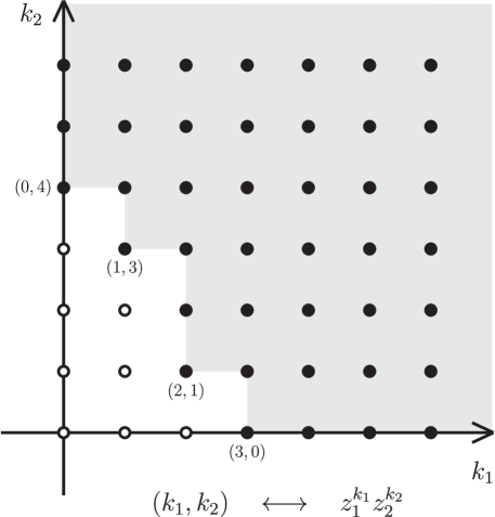
Figure 1: The labeled lattice points are the exponent vectors of the leading term of each element of the Gröbner basis $G$ in eq. (56). The lattice points indicated with white circles are the elements of the set $E$ defined in eq. (26). These elements define exponent vectors of the canonical basis elements.

Hence we find the following exponent vectors of the canonical basis elements,

$$E=\big{\{}(1,2),(0,3),(2,0),(1,1),(0,2),(1,0),(0,1),(0,0)\big{\}}\,.$$ (59)

Thus, the canonical basis takes the following form,

$$\mathcal{C}=\big{(}z_{1}z_{2}^{2},z_{2}^{3},z_{1}^{2},z_{1}z_{2},z_{2}^{2},z_{1},z_{2},1\big{)}\,.$$ (60)

We remark that different choices of monomial order lead to different canonical bases (but of course with the same number of elements). For example, if we choose lexicographic monomial order, we find the following canonical basis,

$$\mathcal{C}_{\mathrm{lex}}=\big{(}z_{1}z_{2}^{3},z_{1}z_{2}^{2},z_{1}z_{2},z_{1},z_{2}^{3},z_{2}^{2},z_{2},1\big{)}\,.$$ (61)

4.2 Computation of dual basis of $Q$

To construct the dual basis of $Q$ wrt. $\mathcal{C}$, we start by computing the Bezoutian matrix of the ideal generators $P_{i}(z)$ in eq. (54). We find, cf. eq. (28),

$$\mathrm{Bez}(z,y)=\left(\begin{array}[]{cc}(y_{1}+z_{1})(z_{2}-1)&y_{1}^{2}\\[8.53581pt] \chi(\chi(y_{1}+z_{1})+2)z_{2}^{3}&(\chi y_{1}+1)^{2}\left(y_{2}^{2}+z_{2}y_{2}+z_{2}^{2}\right)\end{array}\right)\,.$$ (62)

The Bezoutian determinant is thus,

$$\mathcal{B}(z,y) =\chi^{2}y_{1}^{3}\left(y_{2}^{2}(z_{2}-1)+y_{2}(z_{2}-1)z_{2}-z_{2}^{2}\right)$$

$$\hskip 11.38109pt+y_{1}(z_{2}{-}1)\left(y_{2}z_{2}+y_{2}^{2}+z_{2}^{2}\right)(2\chi z_{1}{+}1)+z_{1}(z_{2}{-}1)\left(y_{2}z_{2}+y_{2}^{2}+z_{2}^{2}\right)$$

$$\hskip 11.38109pt+\chi y_{1}^{2}\left(y_{2}^{2}(z_{2}-1)+y_{2}(z_{2}-1)z_{2}-z_{2}^{2}\right)(\chi z_{1}+2)\,.$$ (63)

We now perform polynomial division of $\mathcal{B}(z,y)$ with respect to the Gröbner basis $G$, where the elements are taken as polynomials in the $z_{i}$ variables. This produces the following decomposition, cf. eq. (30),

$$(q_{1},q_{2},q_{3},q_{4}) =\big{(}0,0,0,\textstyle{\frac{1}{2\chi}}+y_{1}\big{)}$$ (64)

$$\mathcal{B}_{Q}(z,y) =(2\chi+\chi^{2}y_{1})\Big{[}y_{1}^{2}\left(y_{2}^{2}(z_{2}-1)+y_{2}(z_{2}-1)z_{2}-z_{2}^{2}\right)$$

$$\hskip 79.66771pt+y_{1}z_{1}\left(y_{2}^{2}(z_{2}-1)+y_{2}(z_{2}-1)z_{2}-z_{2}^{2}\right)-z_{1}^{2}\Big{]}$$

$$\hskip 11.38109pt+(y_{1}+z_{1})\left(y_{2}^{2}(z_{2}-1)+y_{2}(z_{2}-1)z_{2}-z_{2}^{2}\right)-\textstyle{\frac{z_{2}^{3}}{2\chi}}+\textstyle{\frac{3}{2}}\chi z_{1}^{2}\,.$$ (65)

Next we perform polynomial division of the remainder $\mathcal{B}_{Q}(z,y)$ with respect to $G$, where the elements are now taken as polynomials in the $y_{i}$ variables, $P_{i}(z)\to P_{i}(y)$. This produces the decomposition in eq. (31) with

$$(\widehat{q}_{1},\widehat{q}_{2},\widehat{q}_{3},\widehat{q}_{4})=\Big{(}\chi(z_{2}-1)(y_{2}+z_{2}+1)\big{(}\chi(y_{1}+z_{1})+2\big{)},\hskip 3.41432pt\textstyle{\frac{1}{2\chi}},\hskip 1.70717pt0,\hskip 1.70717pt0\Big{)}\,,$$ (66)

where the remainder is $\mathcal{B}_{Q\otimes Q}(z,y)=c_{1}(z)d_{1}(y)+\cdots+c_{D}(z)d_{D}(y)$, with the dual basis elements taking the following form,

$$\mathcal{D} =\Big{(}(z_{2}{-}1)(2\chi z_{1}{+}1),\hskip 4.2679pt-\textstyle{\frac{1}{2\chi}},\hskip 4.2679pt-\chi^{2}z_{1}{-}\textstyle{\frac{\chi}{2}},\hskip 4.2679ptz_{2}(z_{2}{-}1)(2\chi z_{1}{+}1),$$

$$\hskip 22.76219ptz_{1}(z_{2}{-}1),\hskip 4.2679pt-\chi^{2}z_{1}^{2}{-}2\chi z_{1}z_{2}^{2}{-}z_{2}^{2},\hskip 4.2679ptz_{1}z_{2}(z_{2}{-}1),\hskip 4.2679pt-z_{1}z_{2}^{2}{-}\textstyle{\frac{1}{2\chi}}z_{2}^{3}{-}\textstyle{\frac{\chi}{2}}z_{1}^{2}\Big{)}\,,$$ (67)

where we have expressed the elements as functions of the $z_{i}$ variables.

4.3 Constructing partition-of-unity polynomials

To construct the partition-of-unity polynomials in eq. (37), our first aim is to find a linear form which maps the elements $p_{i}$ of the variety (55) to distinct values. We observe that the linear form

$$\ell(z_{1},z_{2})=z_{1}+z_{2}\,,$$ (68)

has this property. From eq. (34) we then obtain the following Lagrange polynomials,

$$(L_{1}(z),L_{2}(z))\hskip 2.84526pt=\hskip 2.84526pt\left(\frac{\chi(z_{1}+z_{2}-1)+1}{1-\chi},\hskip 4.2679pt\frac{\chi(z_{1}+z_{2})}{\chi-1}\right)\,,$$ (69)

and we observe that $L_{i}(p_{j})=\delta_{ij}$, as desired.

Our next aim is to compute $\delta$ as defined in eq. (39). To this end, we first compute $M$, defined in eq. (38) as the intersection of the ideals associated with each pole of the variety. In the case at hand, the ideals associated with each pole of the variety (55) are

$$J\langle\{p_{1}\}\rangle =\langle z_{1},z_{2}\rangle$$ (70)

$$J\langle\{p_{2}\}\rangle =\left\langle z_{1}+\textstyle{\frac{1}{\chi}},z_{2}-1\right\rangle\,.$$ (71)

Accordingly, we introduce the parameter $t$ and compute the Gröbner basis of

$$\big{\langle}tz_{1},tz_{2},(1-t)\big{(}z_{1}+\textstyle{\frac{1}{\chi}}\big{)},(1-t)(z_{2}-1)\big{\rangle}$$ (72)

wrt. lexicographic monomial order and the variable order $(t,z_{1},z_{2})$. We find $\{z_{1}+\frac{z_{2}}{\chi},z_{2}^{2}-z_{2},z_{2}+t-1\}$. The elements which do not contain the parameter $t$ then form a basis of $J\langle\{p_{1}\}\rangle\cap J\langle\{p_{2}\}\rangle$,

$$M=\big{\langle}z_{1}+\textstyle{\frac{z_{2}}{\chi}},z_{2}^{2}-z_{2}\big{\rangle}\,.$$ (73)

Now, to determine $\delta$, we start by checking whether $M\subseteq I$. Polynomial division of the elements of eq. (73) wrt. the Gröbner basis of $I$ in eq. (56) leaves remainders identical to the original elements.

Thus, we proceed to consider $M^{2}$. Taking the products of the generators in eq. (73) and performing polynomial division we find

$$M^{2}=\big{\langle}\big{(}z_{1}+\textstyle{\frac{z_{2}}{\chi}}\big{)}^{2},\hskip 2.84526pt(z_{2}^{2}-z_{2})\big{(}z_{1}+\textstyle{\frac{z_{2}}{\chi}}\big{)},\hskip 2.84526ptz_{2}^{2}-z_{2}^{3}\big{\rangle}\,.$$ (74)

As the remainders are non-zero, we proceed to consider $M^{3}$. Taking the products of the generators in eqs. (73) and (74) and performing polynomial division we find

$$M^{3} =\Big{\langle}\textstyle{\frac{3}{2}}\left(\textstyle{\frac{z_{2}^{3}}{\chi^{3}}}+\textstyle{\frac{2z_{1}z_{2}^{2}}{\chi^{2}}}+\textstyle{\frac{z_{1}^{2}}{\chi}}\right),\hskip 4.2679pt-\textstyle{\frac{z_{2}^{3}}{\chi^{2}}}-\textstyle{\frac{2z_{1}z_{2}^{2}}{\chi}}-z_{1}^{2},\hskip 4.2679pt-\textstyle{\frac{z_{2}^{3}}{\chi^{2}}}-\textstyle{\frac{2z_{1}z_{2}^{2}}{\chi}}-z_{1}^{2},\hskip 4.2679pt$$

$$\hskip 24.18483pt\textstyle{\frac{1}{2}}\left(\textstyle{\frac{z_{2}^{3}}{\chi}}+\chi z_{1}^{2}+2z_{1}z_{2}^{2}\right),\hskip 4.2679pt\textstyle{\frac{1}{2}}\left(\textstyle{\frac{z_{2}^{3}}{\chi}}+\chi z_{1}^{2}+2z_{1}z_{2}^{2}\right),\hskip 4.2679pt0\Big{\rangle}\,.$$ (75)

As the remainders are non-zero, we proceed to consider $M^{4}$. Taking the products of the generators in eqs. (73) and (75) and performing polynomial division we find

$$M^{4}=\langle 0\rangle\,.$$ (76)

Hence we conclude that $\delta=4$.

Alternatively, we may use the maximum pole multiplicity as a value for $\delta$. To this end we compute the matrix $M_{\ell}$ of $P(z)\mapsto\ell(z)P(z)$ for the linear form in eq. (68). Using the canonical basis $\mathcal{C}=(c_{1}(z),\ldots,c_{8}(z))$ in eq. (60), we find

$$M_{\ell}\hskip 2.27621pt=\hskip 2.27621pt\left(\begin{array}[]{cccccccc}0&-\frac{1}{2\chi}&1{-}\frac{\chi}{2}&0&0&0&0&0\\[2.84526pt] 0&1{-}\frac{1}{2\chi}&-\frac{\chi}{2}&0&0&0&0&0\\[2.84526pt] 0&\frac{1}{2\chi^{3}}&1{-}\frac{3}{2\chi}&0&0&0&0&0\\[2.84526pt] 1&0&1&0&0&0&0&0\\ 1&1&0&0&0&0&0&0\\ 0&0&1&1&0&0&0&0\\ 0&0&0&1&1&0&0&0\\ 0&0&0&0&0&1&1&0\\ \end{array}\right)\,,$$ (77)

i.e., so that $\ell(z)c_{i}(z)\equiv\sum_{j=1}^{8}(M_{\ell})_{ij}c_{j}(z)\mbox{ (mod $I$)}$. From this we find

$$\det(\lambda I-M_{\ell})\hskip 2.27621pt=\hskip 2.27621pt\big{(}\lambda-\ell(p_{1})\big{)}^{6}\big{(}\lambda-\ell(p_{2})\big{)}^{2}\,.$$ (78)

We conclude that the poles $p_{1}$ and $p_{2}$ have the multiplicities 6 and 2, respectively. In particular, $d_{\mathrm{max}}=6$.

Plugging the value $\delta=4$ from eq. (76) into eq. (37) with the Lagrange polynomials given in eq. (69) and performing polynomial division wrt. $G$, we find

$$e_{1}(z)=1-z_{2}^{3}\hskip 17.07164pt\mathrm{and}\hskip 17.07164pte_{2}(z)=z_{2}^{3}\,.$$ (79)

It is straightforward to check that these polynomials indeed have the properties stated in eqs. (35)–(36).

Now, to compute the residues at each pole $p_{i}$ in the variety (55), we utilize the partition-of-unity polynomials computed in eq. (79) and consider the numerator of eq. (53), i.e. $h(z)=z_{1}-z_{2}$, multiplied by these polynomials,

$$h(z)e_{1}(z) =(z_{1}-z_{2})(1-z_{2}^{3}) \hskip 2.84526pt\equiv\textstyle{\frac{(2\chi+1)}{2\chi}}z_{2}^{3}+\textstyle{\frac{\chi}{2}}z_{1}^{2}+z_{1}-z_{2} \hskip 17.07164pt\mbox{(mod $I$)}\,,$$ (80)

$$h(z)e_{2}(z) =(z_{1}-z_{2})z_{2}^{3} \hskip 2.84526pt\equiv-\textstyle{\frac{2\chi+1}{2\chi}}z_{2}^{3}-\textstyle{\frac{\chi}{2}}z_{1}^{2} \hskip 17.07164pt\mbox{(mod $I$)}\,.$$

We proceed to decompose these in the canonical basis $\mathcal{C}$ given in eq. (60), finding the following coefficient vectors,

$$\Lambda_{1} =\big{(}0,\textstyle{\frac{2\chi+1}{2\chi}},\frac{\chi}{2},0,0,1,-1,0\big{)}\,,$$ (81)

$$\Lambda_{2} =\big{(}0,-\textstyle{\frac{2\chi+1}{2\chi}},-\frac{\chi}{2},0,0,0,0,0\big{)}\,,$$ (82)

i.e., where $h(z)e_{i}(z)\equiv\Lambda_{i}\cdot\mathcal{C}$ (mod $I$). Moreover, the constant 1 may be composed in the dual basis $\mathcal{D}$ in eq. (67) as $1=\mu\cdot\mathcal{D}$ where,

$$\mu=(0,-2\chi,0,0,0,0,0,0)\,.$$ (83)

Thus we find for the residues,

$$\mathop{\mathrm{Res}}_{I,\hskip 1.70717ptz=p_{1}}\omega \hskip 2.84526pt=\hskip 2.84526pt\Lambda_{1}\cdot\mu \hskip 2.84526pt=\hskip 2.84526pt-2\chi-1\,,$$ (84)

$$\mathop{\mathrm{Res}}_{I,\hskip 1.70717ptz=p_{2}}\omega \hskip 2.84526pt=\hskip 2.84526pt\Lambda_{2}\cdot\mu \hskip 2.84526pt=\hskip 2.84526pt2\chi+1\,.$$

5 Global residue theorems

In this section we discuss global residue theorems for multivariate meromorphic forms. In the univariate case it is well known that the sum of all residues, including that at infinity, equals zero,

$$\sum_{i=1}^{m}\mathop{\mathrm{Res}}_{z=p_{i}}\varpi\hskip 2.84526pt=\hskip 2.84526pt0\,,$$ (85)

where $\{p_{1},\ldots,p_{m}\}\subset\mathbb{CP}^{1}$ denote the poles of $\varpi$.

This property generalizes to the multivariate case,

$$\omega=\frac{h(z)\hskip 1.13809pt{\rm d}z_{1}\wedge\cdots\wedge{\rm d}z_{n}}{f_{1}(z)\cdots f_{n}(z)}\,,$$ (86)

where, however, one typically has several linear relations which relate the residues at finite locations to residues at infinity. The existence of these relations follows from the following theorem.

Theorem 2.

(Global residue theorem). Let $\omega$ denote a meromorphic $n$-form defined on a compact manifold $M$. Given an open covering $\{U_{i}\}$, let $\omega$ take the local form given in eq. (86). Furthermore, let $D_{j}=\{z\in M:f_{j}(z)=0\}$ with $j=1,\ldots,n$ denote the divisors of $\omega$, and assume that $V=D_{1}\cap\cdots\cap D_{n}$ is a finite set. Then

$$\sum_{p\in V}\mathop{\mathrm{Res}}_{p}\omega\hskip 2.84526pt=\hskip 2.84526pt0\,,$$ (87)

where each $\mathop{\mathrm{Res}}_{p}\omega$ is evaluated locally on a patch $U_{i}$ which contains $p$.

For a proof we refer to section 5.1 of ref. [21].

As the global residue theorem applies to forms defined on compact manifolds, in order to apply it to an $n$-form defined on $\mathbb{C}^{n}$, one must add a boundary at infinity. One convenient way to do so is to embed $\mathbb{C}^{n}$ in complex projective space $\mathbb{CP}^{n}$, which is compact. In the following we will show how to apply the global residue theorem for this choice of compactification. However, we emphasize that other compactifications exist, corresponding to alternative ways of adding a boundary at infinity, and will lead to different residue relations produced by the global residue theorem.

We recall that $\mathbb{CP}^{n}$ can be defined as the space of $(n+1)$-tuples of complex numbers $W=(w_{0},\ldots,w_{n})\in\mathbb{C}^{n+1}\setminus\{0\}$ where two elements are identified if they lie along the same line passing through the origin, $tW\sim W$ for $t\in\mathbb{C}\setminus\{0\}$. That is,

$$\mathbb{CP}^{n}=\{(w_{0},\ldots,w_{n})\neq 0\}\Big{/}\{tW\sim W\hskip 5.69054pt\mathrm{where}\hskip 5.69054ptt\neq 0\}\,.$$ (88)

A covering of $\mathbb{CP}^{n}$ is provided by the patches

$$U_{i}=\{(w_{0},\ldots,w_{n})\hskip 2.27621pt:\hskip 2.27621ptw_{i}=1\}\hskip 11.38109pt\mathrm{where}\hskip 11.38109pti=0,\ldots,n\,.$$ (89)

Here $\mathbb{C}^{n}=\{(z_{1},\ldots,z_{n})\}$ can be identified with the patch $U_{0}$ by using the homogeneous coordinates,

$$z_{1}=\frac{w_{1}}{w_{0}}\,,\hskip 8.53581pt\ldots,\hskip 8.53581ptz_{n}=\frac{w_{n}}{w_{0}}\,,$$ (90)

since on patch $U_{0}$ we have $w_{0}=1$. Thus, $\mathbb{C}^{n}\subset\mathbb{CP}^{n}$. Points with $w_{0}=0$ are referred to as points at infinity. For the Riemann sphere $\mathbb{CP}^{1}$, the patches $U_{0}$ and $U_{1}$ are the Riemann sphere with respectively the point at infinity $(0,1)$, and the origin $(1,0)$, removed.

To define the differential form in eq. (86) on each of the patches $U_{k}$ in eq. (89) we must find the Jacobian from the coordinates $(z_{1},\ldots,z_{n})$ to $(w_{0},\ldots,w_{k-1},w_{k+1},\ldots,w_{n})$. Using the homogeneous coordinates in eq. (90), it is straightforward to show that

$$\mathop{\mathrm{det}}_{\begin{subarray}{c}i\in\{1,\ldots,n\}\phantom{\setminus\{k\}}\\ j\in\{0,\ldots,n\}\setminus\{k\}\end{subarray}}\frac{\partial z_{i}}{\partial w_{j}}\hskip 5.69054pt=\hskip 5.69054pt\frac{(-1)^{k}}{w_{0}^{n+1}}\,.$$ (91)

Letting $\widehat{{\rm d}w_{k}}$ denote that the respective differential has been dropped, we therefore find that $\omega$ evaluated on the patch $U_{k}$ takes the form,

$$\omega\big{|}_{U_{k}}\hskip 2.84526pt=\hskip 2.84526pt\frac{(-1)^{k}\hskip 0.85358pth\big{(}\textstyle{\frac{w}{w_{0}}}\big{)}\hskip 1.13809pt{\rm d}w_{0}\wedge\cdots\wedge\widehat{{\rm d}w_{k}}\wedge\cdots\wedge{\rm d}w_{n}}{w_{0}^{n+1}f_{1}\big{(}\textstyle{\frac{w}{w_{0}}}\big{)}\cdots f_{n}\big{(}\textstyle{\frac{w}{w_{0}}}\big{)}}\,.$$ (92)

To apply the global residue theorem, we must then consider each partition of the factors contained in the set $\{w_{0}^{n+1},f_{1}\big{(}\textstyle{\frac{w}{w_{0}}}\big{)},$ $\ldots,f_{n}\big{(}\textstyle{\frac{w}{w_{0}}}\big{)}\}$ into $n$ divisors. Each partition gives rise to a linear relation, as we will see in the following example.

5.1 Example: application of the global residue theorem

To illustrate how the global residue theorem (theorem 2) yields linear relations between the residues of a meromorphic form, we consider as an example the form $\omega$ given in eq. (9). Expressed in terms of the homogeneous coordinates (90), $\omega$ takes the following form on patch $U_{k}$,

$$\omega\big{|}_{U_{k}}\hskip 2.84526pt=\hskip 2.84526pt\frac{(-1)^{k}\hskip 1.13809ptw_{1}\hskip 1.70717pt{\rm d}w_{0}\wedge\cdots\wedge\widehat{{\rm d}w_{k}}\wedge\cdots\wedge{\rm d}w_{2}}{w_{0}w_{2}(a_{1}w_{1}+a_{2}w_{2})(b_{1}w_{1}+b_{2}w_{2})}\,.$$ (93)

In this case there are seven distinct partitions of the four denominator factors. Let us consider the following partition,

$$f_{1}(w)=w_{0}w_{2}\,,\hskip 11.38109ptf_{2}(w)=(a_{1}w_{1}+a_{2}w_{2})(b_{1}w_{1}+b_{2}w_{2})\,,$$ (94)

giving rise to the divisors $D_{i}=\{(w_{0},w_{1},w_{2})\hskip 0.85358pt:\hskip 0.85358ptf_{i}(w)=0\}$. We find that the intersection of the divisors is a finite set,

$$V=D_{1}\cap D_{2}=(p_{1},p_{2},p_{3})=\Big{(}(1,0,0),\big{(}0,1,-\textstyle{\frac{a_{1}}{a_{2}}}\big{)},\big{(}0,1,-\textstyle{\frac{b_{1}}{b_{2}}}\big{)}\Big{)}\,,$$ (95)

and hence the global residue theorem applies. Noting that $p_{1}\in U_{0}$ and $p_{2,3}\in U_{1}$, we can evaluate the residues on these respective patches, dropping the constant $w_{0}$ and $w_{1}$ entries, respectively. For the left-hand side of eq. (87) we then find,

$$\sum_{p\in V}\mathop{\mathrm{Res}}_{p}\omega =\mathop{\mathrm{Res}}_{I_{0};\hskip 0.85358ptp_{1}}\frac{w_{1}\hskip 1.70717pt{\rm d}w_{1}\wedge{\rm d}w_{2}}{w_{2}(a_{1}w_{1}{+}a_{2}w_{2})(b_{1}w_{1}{+}b_{2}w_{2})}+\mathop{\mathrm{Res}}_{I_{1};\hskip 0.85358ptp_{2}}\frac{(-1)\hskip 1.70717pt{\rm d}w_{0}\wedge{\rm d}w_{2}}{w_{0}w_{2}(a_{1}{+}a_{2}w_{2})(b_{1}{+}b_{2}w_{2})}$$

$$\hskip 14.22636pt+\mathop{\mathrm{Res}}_{I_{1};\hskip 0.85358ptp_{3}}\frac{(-1)\hskip 1.70717pt{\rm d}w_{0}\wedge{\rm d}w_{2}}{w_{0}w_{2}(a_{1}{+}a_{2}w_{2})(b_{1}{+}b_{2}w_{2})}\,,$$ (96)

where the residues are computed with respect to the ideals $I_{j}\equiv\big{\langle}f_{1}(w),f_{2}(w)\big{\rangle}\big{|}_{w_{j}=1}$ for $j=0,1$. Explicitly, we find

$$\sum_{p\in V}\mathop{\mathrm{Res}}_{p}\omega\hskip 2.84526pt=\hskip 2.84526pt-\frac{1}{a_{1}b_{1}}-\frac{a_{2}}{a_{1}(a_{1}b_{2}-a_{2}b_{1})}-\frac{b_{2}}{b_{1}(a_{2}b_{1}-a_{1}b_{2})}\hskip 2.84526pt=\hskip 2.84526pt0\,,$$ (97)

in agreement with eq. (87).

Analogously, for the partition

$$f_{1}(w)=w_{0}(a_{1}w_{1}+a_{2}w_{2})\,,\hskip 11.38109ptf_{2}(w)=w_{2}(b_{1}w_{1}+b_{2}w_{2})\,,$$ (98)

we have

$$V=\Big{(}(1,0,0),\big{(}0,1,0\big{)},\big{(}0,1,-\textstyle{\frac{b_{1}}{b_{2}}}\big{)}\Big{)}\,,$$ (99)

and obtain the residue relation,

$$\sum_{p\in V}\mathop{\mathrm{Res}}_{p}\omega\hskip 2.84526pt=\hskip 2.84526pt-\frac{a_{2}}{a_{1}(a_{1}b_{2}-a_{2}b_{1})}-\frac{1}{a_{1}b_{1}}-\frac{b_{2}}{b_{1}(a_{2}b_{1}-a_{1}b_{2})}\hskip 2.84526pt=\hskip 2.84526pt0\,,$$ (100)

again in agreement with eq. (87).

The global residue theorems associated with the remaining five partitions of the denominator factors of $\omega$ are computed analogously.

6 Applications of multivariate residues

In this section we give two applications of multivariate residues, namely the computation of generalized-unitarity cuts and the Cachazo-He-Yuan scattering equations. The former are important in several contexts, for example unitarity calculations of loop amplitudes and the Grassmannian formulation of the S-matrix by Arkani-Hamed et al.

First we focus on unitarity calculations. To provide some context, let us consider a one-loop scattering amplitude in a generic gauge theory. From standard reduction techniques it can be shown that there is a finite basis of one-loop integrals in which the amplitude can be expanded [25, 26, 27],

$$A^{(1)}_{n}=\sum_{\mathrm{boxes}}c_{\Box}I_{\Box}+\sum_{\mathrm{triangles}}c_{\triangle}I_{\triangle}+\sum_{\mathrm{bubbles}}c_{\circ}I_{\circ}+\sum_{\mathrm{tadpoles}}c_{\multimap}I_{\multimap}+\mbox{rational terms}\,,$$ (101)

where $I_{\Box},I_{\triangle},I_{\circ}$ and $I_{\multimap}$ represent box, triangle, bubble and tadpole integrals, respectively. As all these integrals are known [28], this decomposition reduces the computation of $A^{(1)}_{n}$ to the computation of the expansion coefficients.

The coefficient $c_{\Box}$ of the box integral

$$I_{\Box}=\int_{\mathbb{R}^{D}}\frac{{\rm d}^{D}\ell}{(2\pi)^{D}}\frac{1}{\prod_{i=1}^{4}p_{i}^{2}(\ell)}\,,$$ (102)

can now be computed by replacing the integration contour $\mathbb{R}^{D}$ in eq. (101) by the contour

$$T^{4}_{\epsilon}=\{\ell\in\mathbb{C}^{4}:|p^{2}_{i}(\ell)|=\epsilon_{i},\hskip 7.11317pti=1,\ldots,4\}\,.$$ (103)

The replacement of contour $\mathbb{R}^{D}\to T^{4}_{\epsilon}$ has the effect of computing the residue at the poles where all four propagators $p_{i}^{2}(\ell)$ of $I_{\Box}$ go on shell. All terms missing any one of the propagators therefore vanish, and eq. (101) becomes [29]

$$c_{\Box}=\frac{1}{2}\sum_{a\in\{L,L^{\bullet}\}}\sum_{{\mathrm{helicities,}\atop\mathrm{species}}}\prod_{i=1}^{4}\hskip 1.13809ptA^{\mathrm{tree}}_{i}\big{(}p_{i}(a),p_{i+1}(a)\big{)}\,,$$ (104)

where $L,L^{\bullet}$ denote the solutions to $p_{i}^{2}(\ell)=0$ for $i=1,\ldots,4$, and $A^{\mathrm{tree}}_{i}$ are the tree amplitudes arising from literally cutting the propagators of the box graph.

More to the point, though the integral $\int_{T^{4}_{\epsilon}}\frac{{\rm d}^{D}\ell}{(2\pi)^{D}}\frac{1}{\prod_{i=1}^{4}p_{i}^{2}(\ell)}$ is a multivariate residue, it is non-degenerate and can thus be computed directly from eq. (5). However, starting at two loops, degenerate residues are generic, and the algorithms explained in sections 2.1 and 3 become necessary to evaluate them. To give an explicit example, we consider the generalized-unitarity cut shown in figure 2.

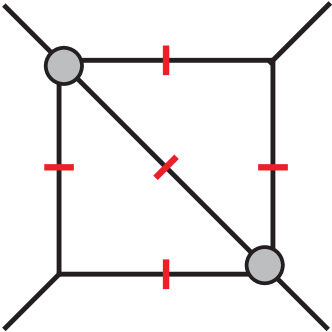
Figure 2: (Color online.) A generalized-unitarity cut where the propagators with superimposed red lines have been put on shell. The gray blobs represent tree amplitudes.

It turns out that the five on-shell constraints can be integrated out as a non-degenerate residue. However, the residues of the resulting integrand in the remaining $2\times 4-5=3$ variables will generically be degenerate: for example, the residue with respect to the ideal $I$ (where $\chi$ denotes the ratio $t/s$ of Mandelstam invariants),

$$I=\langle z_{1}^{2},\hskip 1.99168ptz_{2},\hskip 1.99168pt-\chi z_{1}+\chi z_{3}z_{1}+z_{3}z_{1}+z_{2}z_{3}-z_{3}\rangle\,,$$ (105)

at $(z_{1},z_{2},z_{3})=(0,0,0)$ is degenerate, and the algorithms explained in sections 2.1 and 3 are required to compute the residue.

Multivariate residues also play a central role in the Cachazo-He-Yuan scattering equations which describe tree-level scattering amplitudes in any spacetime dimension [30]. In this formalism, the scattering of $n$ particles with momenta $p_{a}$ is encoded in the solutions $\sigma_{a}\in\mathbb{CP}^{1}$ to the scattering equations,

$$\sum_{b\neq a}\frac{s_{ab}}{\sigma_{a}-\sigma_{b}}=0\,,$$ (106)

where $s_{ab}=(p_{a}+p_{b})^{2}$ denote Mandelstam invariants. If the solutions to these equations can be found, the tree-level amplitude in any dimension can then be computed as,

$$A_{n}=\int\frac{{\rm d}^{n}\sigma}{\mathrm{vol}\hskip 1.70717ptSL(2,\mathbb{C})}\prod_{a}{}^{\prime}\hskip 2.56073pt\delta\left(\textstyle{\sum_{b\neq a}\frac{s_{ab}}{\sigma_{ab}}}\right)\frac{E_{n}(\{p,\epsilon,\sigma\})}{\sigma_{12}\sigma_{23}\cdots\sigma_{n1}}\,,$$ (107)

where $\sigma_{ij}\equiv\sigma_{i}-\sigma_{j}$, $\epsilon$ denotes polarization vectors, and the prime on the product sign indicates that (any) three of the equations are dropped (as only $n-3$ equations are independent). The quantity $E_{n}$ depends on the underlying theory (for Yang-Mills theory, it is the Pfaffian of an antisymmetric matrix composed of all dot products of $k_{i}$ and $\epsilon_{j}$, divided by $\sigma_{ab}$). The delta functions are more properly understood as contour integrals.

In practice, obtaining the $(n-3)!$ solutions to eq. (106) is difficult, and summing over the individual residues at each pole $\sigma_{ab}$ in eq. (107) is not straightforward for high multiplicities $n$. However, as observed in refs. [31, 32], these steps can be circumvented by directly computing the global residue (23). In practice this leads to an efficient method for computing tree amplitudes in the Cachazo-He-Yuan formalism.

MultivariateResidues allows direct computation of the global residue. As a result, the package enables direct evaluation of tree amplitudes in the Cachazo-He-Yuan formalism, bypassing the steps of solving eq. (106) and summing over the individual residues. In section 7.4 we illustrate this by computing the five-scalar tree amplitude in $\phi^{3}$ theory.

We remark that multivariate residues also play an important role in elimination theory in the context of solving systems of multivariate polynomial equations [19].

7 Manual

The package MultivariateResidues.m can be obtained from ref. [33]. At the beginning of a Mathematica session, the package can be loaded with

⬇

<< ”MultivariateResidues‘”

where it is assumed that the package and the notebook are located in the same directory. The newly available definitions can be shown by running

The package defines one new function, called MultivariateResidue. Below we give a brief introduction to this function and its options.

7.1 New functions

The function MultivariateResidue computes a multivariate residue, based on the algorithms described in this paper. It has the following syntax:

⬇

{z[1] -> z[1,1], …, z[n] -> z[n,1]}]

which returns the multivariate residue of $\mathrm{Num}/(d_{1}\,d_{2}\dotsm d_{n})$ at the location given by $(z_{1},\dotsc,z_{n})=(z_{1}^{(1)},\dotsc,z_{n}^{(1)})$. Alternatively,

⬇

{{z[1,1], …, z[n,1]}, {z[1,2], …, z[n,2]}, …}]

returns a list of multivariate residues of $\mathrm{Num}/(d_{1}\,d_{2}\dotsm d_{n})$ at the collection of points $(z_{1},\dotsc,z_{n})\in\{(z_{1}^{(1)},\dotsc,z_{n}^{(1)}),(z_{1}^{(2)},\dotsc,z_{n}^{(2)}),\dotsc\}$. This second syntax is better suited for the computation of several residues, because it exploits the fact that part of the computation is common to all poles.

In the univariate case, MultivariateResidue is equivalent to the native Mathematica function Residue. For instance,

⬇

Residue[f[z]/z, {z, 0}]

Out: f[0]

Out: f[0]

As a multivariate example, let us compute the residues considered in section 2.1. Taking $\varphi_{1},\varphi_{2},\varphi_{3}$ from eq. (10), we can straightforwardly compute the residues with respect to the ideals given in eq. (11) as follows:

⬇

f[2] = a[1] z[1] + a[2] z[2];

f[3] = b[1] z[1] + b[2] z[2];

MultivariateResidue[z[1], {f[1], f[2]*f[3]}, {z[1] -> 0, z[2] -> 0}]

MultivariateResidue[z[1], {f[2], f[3]*f[1]}, {z[1] -> 0, z[2] -> 0}]

MultivariateResidue[z[1], {f[3], f[1]*f[2]}, {z[1] -> 0, z[2] -> 0}]

Out: -(1/(a[1] b[1]))

Out: -(a[2]/(a[1] (-a[2] b[1] + a[1] b[2])))

Out: -(b[2]/(b[1] (a[2] b[1] - a[1] b[2])))

When using the second syntax, the input list of poles does not have to contain all points in the variety defined by the ideal (i.e., the set of points where all denominator factors vanish). Moreover, it may contain additional points (although the corresponding residues will be zero). As an example, consider the following ideal,

⬇

z[2]^3 (-1 - z[1] - a z[1] + z[2] + a z[1] z[3])};

Parameters = {a};

Vars = {z[1], z[2], z[3]};

The resulting variety contains three points,

⬇

Out: {{-1, 0, 0}, {0, 0, 0}, {0, 1, 0}}

We may ask for the residue computed at precisely the poles contained in the variety, or alternatively a subset, or alternatively a subset with an added random point,

⬇

MultivariateResidue[1, Ideal, Vars, Variety[[1 ;; 2]]]

MultivariateResidue[1, Ideal, Vars, Join[Variety[[1 ;; 2]], {{0, 0, 1}}]]

Out: {-(6/a), 0, 6/a}

Out: {-(6/a), 0}

Out: {-(6/a), 0, 0}

In fact, the algorithm based on the dual structure of the quotient ring requires the computation of the residues of all poles in the variety. This particular algorithm will therefore internally compute the variety itself and return the residues at the (sub)set of poles that are specified by the user.

When using the method "QuotientRingDuality" one may also specify Variety = {GlobalResidue}. In this case the program returns the global residue (23), which equals the sum of all local residues. The benefit is that the global residue can be calculated directly without determining the partition-of-unity polynomials $e_{i}$ in eq. (36) required to compute the local residues. We refer to section 7.4 for an example.

MultivariateResidues contains an implementation of the global residue theorem discussed in section 5, choosing to extend the input differential form $\omega$ to complex projective space $\mathbb{CP}^{n}$. The syntax is

where Num denotes the numerator of $\omega$, Ideal the denominator factors and Vars the variables.

As an example, let us consider the differential form in section 5.1,

⬇

Ideal={z[2] (a[1] z[1] + a[2] z[2]), (b[1] z[1] + b[2] z[2])};

Vars={z[1], z[2]};

GRTs=GlobalResidueTheoremCPn[Num, Ideal, Vars];

There are seven linear relations that arise from the global residue theorem,

⬇

Out: 7

The relations are recorded in the form $\{P,\{V,R\}\}$, where $P$ denotes the denominator partition, $V$ the set of poles involved in the relation and $R$ their respective residues. For the denominator partition computed in detail in section 5.1 we have

⬇

Out: {{w[0] w[2], (a[1] w[1] + a[2] w[2]) (b[1] w[1] + b[2] w[2])}, {{{1, 0, 0}, {0, 1, -(a[1]/a[2])}, {0, 1, -(b[1]/b[2])}}, {-(1/(a[1] b[1])), -(a[2]/(a[1] (-a[2] b[1] + a[1] b[2]))), -(b[2]/(b[1] (a[2] b[1] - a[1] b[2])))}}}

It is easy to check that the residues indeed sum to zero,

⬇

Out: 0

GlobalResidueTheoremCPn only records non-vanishing residues and their respective poles. In cases where all the residues that appear in a global residue theorem vanish, the empty set is returned as output.

⬇

Out: {{{w[2], -w[0]^2 + w[1] w[2]}, {{}, {}}}}

7.2 Options

The following options can be specified in MultivariateResidue:

$\bullet$ Method: the type of algorithm used for computing multivariate residues. Possible settings for this option are "TransformationFormula" (default) and "QuotientRingDuality", described in sections 2.1 and 3, respectively.

$\bullet$ CoefficientDomain: the type of objects assumed to be coefficients of monomials in the computation of Gröbner bases. Possible settings for this option are InexactNumbers, Rationals and RationalFunctions (default).

$\bullet$ MonomialOrder: the criterion used for monomial ordering in Gröbner basis computation and polynomial division. This option has an effect when using the method "TransformationFormula" with $MultiResUseSingular=True, or when using "QuotientRingDuality". Possible values are Lexicographic (default), DegreeLexicographic and DegreeReverseLexicographic.

$\bullet$ FindMinimumDelta: compute and use the smallest possible $\delta$ entering the partition-of-unity polynomials $e_{i}=1-(1-L_{i}^{\delta})^{\delta}$, which are needed to compute residues at all the finite poles of the variety. Possible settings are True (default) and False. Specifying True will compute and use the smallest possible $\delta$; specifying False will drop the calculation of a minimal $\delta$ and use a generally larger value (namely the maximum pole multiplicity).

7.3 Global Settings

The following global settings can be specified in a Mathematica session that makes use of the package (the settings can be altered after loading the package and will impact all subsequent MultivariateResidue evaluations):

$\bullet$ $MultiResInputChecks: check the input of MultivariateResidue. It checks for instance whether the ideal is zero-dimensional. Possible values are True (default) and False. It can be switched off to improve efficiency.

$\bullet$ $MultiResInternalChecks: perform internal cross-checks, for instance on the correctness of the transformation matrix $A(z)$ and the partition of unity $e(i)$. Possible values are True (default) and False. Similarly, this can also be switched off to improve efficiency.

$\bullet$ $MultiResUseSingular: use Singular for computations of Gröbner bases and polynomial division. Possible settings are True and False (default). When set to True, one must specify the path to the Singular executable in the variable $MultiResSingularPath. Singular is a computer algebra system dedicated to computational algebraic geometry that can outperform Mathematica for complicated calculations (see section 7.5) and therefore merits an interface between the two programs. Singular is free software under the GNU General Public Licence. It may be obtained from https://www.singular.uni-kl.de.

$\bullet$ $MultiResSingularPath: the path to Singular. By default the path is set to "/usr/bin/Singular".

7.4 Example of application: Cachazo-He-Yuan scattering equations

As discussed in section 6, multivariate residues play a central role in the Cachazo-He-Yuan scattering equations which describe tree-level scattering amplitudes in any spacetime dimension [30]. In this formalism, an $n$-particle amplitude is expressed as the $(n-3)$-fold contour integral in eq. (107) which localizes the integrand to the solution of the scattering equations (106).

As observed in refs. [31, 32], the steps of solving eq. (106) and summing over the individual residues can be circumvented by directly computing the global residue (23).

MultivariateResidues allows direct computation of the global residue and thus in turn tree amplitudes. To illustrate this, we consider the five-scalar tree amplitude in $\phi^{3}$ theory. Following ref. [31], we enter the following input,

⬇

h[2] = s[123]c[3] + s[124]c[4] + s[134]c[3]c[4];

gt[1] = (s[13]s[124] + s[13]s[134] - s[14] (s[123] + s[134]c[4]))/

((s[12] + s[13]) (s[124] + s[134]) - s[14]s[123]);

gt[2] = -((s[12]s[13]s[134] - (s[13] + s[14]) (s[13]s[124]

-s[14] (s[123] + s[134]c[4])))/

(s[12] (s[12]s[134] - (s[13] + s[14]) (s[123] + s[124]))));

gt[3] = (s[13] (s[124] + s[134]c[3]) - s[14]s[123])/(s[12]s[123]);

Vars = {c[3], c[4]};

Num = c[3] (1 - c[4]) gt[1] gt[2] gt[3];

Ideal = {h[1], h[2]};

where (h[a], s[1a], s[1ab], c[a], gt[a], Num) correspond respectively to $(h_{a},\sigma_{a},\sigma_{ab},z_{a},\widetilde{g}_{a},N(z_{3},z_{4}))$ given in eqs. (3.5), (3.10)–(3.13) of ref. [31]. In the above, s[1a] and s[1ab] represent $(p_{1}+p_{a})^{2}$ and $(p_{1}+p_{a}+p_{b})^{2}$. The functions h[a] represent the $n-3=2$ scattering equations (106) in polynomial form, whereas gt[a] represent multiplicative inverses to the Parke-Taylor denominator factors in the integration measure.

The five-scalar amplitude can now be computed as a global residue,

⬇

Out: (s[12]s[13]s[123]s[124] + s[12]s[14]s[123]s[124] + s[13]s[14]s[123]s[124] + s[14]^2 s[123]s[124] - s[13]^2 s[124]^2 - s[13]s[14]s[124]^2 + s[12]s[13]s[123]s[134] + s[12]s[13]s[124]s[134] - s[13]^2 s[124]s[134] - s[13]s[14]s[124]s[134] + s[12]s[13]s[134]^2)/ (s[12]s[123] (-s[13]s[123] - s[14]s[123] - s[13]s[124] - s[14]s[124] + s[12]s[134]) (-s[14]s[123] + s[12]s[124] + s[13]s[124] + s[12]s[134] + s[13]s[134]))

By applying momentum conservation identities, the output expression can be brought into the form,

$$A_{5}^{\mathrm{tree},\hskip 1.70717pt\phi^{3}}=\frac{1}{s_{12}s_{34}}+\frac{1}{s_{23}s_{51}}+\frac{1}{s_{12}s_{45}}+\frac{1}{s_{34}s_{51}}+\frac{1}{s_{23}s_{45}}\,,$$ (108)

which is manifestly the correct expression for the five-scalar tree amplitude in $\phi^{3}$ theory.

7.5 Performance

The speed performance of MultivariateResidue depends on the selected options and global settings; in particular the options Method, MonomialOrder and $MultiResUseSingular. This section demonstrates the impact of these options through a few explicit examples.

The default method "TransformationFormula" is typically the best choice for simple problems, whereas the sophisticated "QuotientRingDuality" can offer speed improvements in more involved computations. For instance, the default method is the fastest method for the residue computation with the simple ideal defined in section 7.1,

⬇

First[AbsoluteTiming[MultivariateResidue[1, Ideal, Vars, Variety, Method -> ”QuotientRingDuality”]]]

Out: 0.255931

Out: 4.147544

On the other hand, if we consider an example with more variables, then the default method becomes less efficient (due to the costly computation of the transformation matrix), and one might opt for "QuotientRingDuality",

⬇

Ideal = Table[z[i], {i, 1, n}];

Vars = Table[z[i], {i, 1, n}]

Variety = {Table[0, {n}]};

First[AbsoluteTiming[MultivariateResidue[1, Ideal, Vars, Variety, Method -> ”TransformationFormula”]]]

First[AbsoluteTiming[MultivariateResidue[1, Ideal, Vars, Variety, Method -> ”QuotientRingDuality”]]]

Out: 1.029218

Out: 0.123257

Another circumstance under which "QuotientRingDuality" performs better than "TransformationFormula" is when points in the variety are large rational functions of one or more parameters. In such cases, the computation of Gröbner bases in "TransformationFormula" can be rather slow. The following example with two complex variables illustrates this point.

⬇

Vars = {z[1], z[2]};

Variety = Map[Last, Sort[Solve[Ideal == 0, Vars]], {2}]

Out: {{-((c[2] - c[4])/(c[2] c[3] - c[1] c[4])), -((-c[1] + c[3])/(c[2] c[3] - c[1] c[4]))}}

For this problem, the "QuotientRingDuality" method is faster,

⬇

First[AbsoluteTiming[MultivariateResidue[1, Ideal, Vars, Variety, Method -> ”QuotientRingDuality”]]]

Out: 0.156636

Out: 0.074859

The method "QuotientRingDuality" also allows the use of various monomial orderings in the computation of Gröbner bases, which can impact the speed of subsequent polynomial reductions. Considering once again the ideal defined in section 7.1 and computing the multivariate residue using three different monomial orderings,

⬇

z[2]^3 (-1 - z[1] - a z[1] + z[2] + a z[1] z[3])};

Vars = {z[1], z[2], z[3]};

Variety = Map[Last, Sort[Solve[Ideal == 0, Vars]], {2}];

First[AbsoluteTiming[MultivariateResidue[1, Ideal, Vars, Variety, Method -> ”QuotientRingDuality”, MonomialOrder -> #]]] & /@ {Lexicographic, DegreeLexicographic, DegreeReverseLexicographic}

Out: {4.128913, 1.459281, 1.733149}

shows that the options DegreeLexicographic and DegreeReverseLexicographic are noticeably faster than Lexicographic. The reason for the speed difference (which becomes more pronounced upon raising the powers of factors in the ideal) is that the Lexicographic monomial ordering produces a Gröbner basis for the ideal which contains only four polynomials (with $2,3,4$ and $16$ terms), whereas the other two monomial orderings produce a Gröbner basis for this ideal with eight polynomials (with $2,2,3,3,4,5,16$ and $19$ terms). The polynomial reduction is faster when using the larger Gröbner basis.

Figure 3 shows the cumulative evaluation time of residues with the various options of MultivariateResidue for the case of a four-gluon two-loop integrand arising after the pentacut shown in figure 2 has been applied. In such problems, where one faces many residue computations, a straightforward way to decrease the total running time is by performing the computations in parallel. This can be achieved by including

and making use of the function ParallelMap. (No parallelization was used in producing figure 3.)

Finally, it is worth mentioning that multivariate residue calculations can be simplified – where possible – by appropriate use of partial fractioning. Suppose one computes the residues of $R(z_{1},z_{2})=(z_{1}f_{1}+z_{2}f_{3})/(f_{1}\,f_{2}\,f_{3}\,f_{4})$, where $f_{i}=a_{i}z_{1}+b_{i}z_{2}$, with respect to the ideal $I(z_{1},z_{2})=\langle\,f_{1}f_{2}\,,f_{3}f_{4}\,\rangle$. A direct computation of the residue yields

⬇

Res[1] = MultivariateResidue[z[1] f[1] + z[2] f[3], {f[1] f[2], f[3] f[4]}, {z[1] -> 0, z[2] -> 0}]

Out: -((a[3] a[4] b[2] + a[4] b[1] b[2] - a[2] a[4] b[3] - a[1] b[2] b[4])/((a[3] b[2] - a[2] b[3]) (a[4] b[1] - a[1] b[4]) (a[4] b[2] - a[2] b[4])))

Partial fractioning the rational function produces two terms, $R(z_{1},z_{2})=z_{1}/(f_{2}\,f_{3}\,f_{4})+z_{2}/(f_{1}\,f_{2}\,f_{4})$. The residue of each of these terms should be computed with respect to the corresponding reduced ideals $\langle\,f_{2}\,,f_{3}f_{4}\,\rangle$ and $\langle\,f_{1}f_{2}\,,f_{4}\,\rangle$. The sum of these two residues reproduces the result of the direct computation,

⬇

Res[2, 2] = MultivariateResidue[z[2], {f[1] f[2], f[4]}, {z[1] -> 0, z[2] -> 0}]

Simplify[Res[1] == Res[2, 1] + Res[2, 2]]

Out: -(b[2]/((a[3] b[2] - a[2] b[3]) (a[4] b[2] - a[2] b[4])))

Out: -(a[4]/((a[4] b[1] - a[1] b[4]) (a[4] b[2] - a[2] b[4])))

Out: True

and is faster than the direct computation (in this case 0.0882 seconds versus 0.4014 seconds).

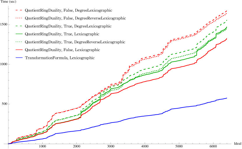
Figure 3: (Color online.) The cumulative evaluation time of residues (vertical axis) over the set of 6395 ideals (horizontal axis) associated with the pentacut of a generic gauge theory two-loop four-gluon integrand for the different residue computation options in the package MultivariateResidues. The legend items are ordered by descending total computation time. The plateaus present in "QuotientRingDuality" show that the underlying computational procedure is sensitive to the precise structure of the ideal. In contrast, "TransformationFormula" exhibits a more linear profile, showing that the underlying computational procedure is less sensitive to the precise structure of the ideal. We also performed these computations with $MultiResUseSingular=True, which increased performance by 18% on average. (Color online. These timings were obtained on a single laptop with 8 GB RAM and 1.8 GHz Intel Core i5 processor.)

8 Conclusions

In this paper we have introduced the Mathematica package MultivariateResidues for the evaluation of multivariate residues. The implementation can be used to compute any multivariate residue of any rational form, including the case where the denominator ideal involves parameters (corresponding, for example, to Lorentz invariants of external momenta in a scattering process).

We have implemented two different algorithms for the computation of residues, one ("TransformationFormula") based on the transformation formula and one ("QuotientRingDuality") exploiting that the residue map defines a non-degenerate inner product on the quotient ring.

We have applied our code to 6500 examples arising in the computation of generalized-unitarity cuts of two-loop scattering amplitudes. From doing so, we have observed the following patterns regarding the relative performance of the two algorithms. In cases where the ideals involve only few parameters, and the expressions of the parameters are polynomials of low degree, "TransformationFormula" is the faster option. Moreover, when the cumulative computation time of "TransformationFormula" is plotted against the range of ideals over which it has been applied, it displays a more linear profile than "QuotientRingDuality", showing that the underlying computational procedure is rather insensitive to the precise structure of the ideal.

In contrast, "QuotientRingDuality" tends to perform better in more involved computations because this circumvents the need to compute the transformation matrix $A(z)$ in eq. (6). This becomes increasingly apparent in cases with several variables, or with several parameters, or whenever ideals involve high-degree polynomials in the parameters.

Appendix A Topology of multivariate residues

In this appendix we aim to explain the underlying topological reason why the value of a multivariate residue is not uniquely determined by the pole enclosed by the integration cycle, but also depends on the cycle. To gain a concrete understanding, we will consider the example of the differential form $\omega$ in eq. (9). The presentation here is largely based on that of section II B of ref. [6] by one of the present authors.

As computed in section 2.1, the differential form (9) has the three distinct residues at $p=(0,0)$ given in eqs. (17)–(19). As we will see shortly, this is reflected in the fact that there are several distinct integration cycles based at $p$ which yield distinct residues. The higher-dimensional situation is thus quite different from contour integration in one complex variable, where a contour either encloses a pole or doesn’t, and there is a unique value for the residue.

To clarify the situation, we seek to split eq. (9) into terms with two distinct denominator factors. To this end, we make the following change of variables,

$$z_{1}^{\prime} =a_{1}z_{1}+a_{2}z_{2}$$ (109)

$$z_{2}^{\prime} =z_{2}\,.$$

After applying this transformation and dropping the primes on $z_{i}$, the form then becomes,

$$\omega=\frac{1}{a_{1}}\left(\frac{1}{z_{2}(c_{1}z_{1}+c_{2}z_{2})}-\frac{a_{2}}{z_{1}(c_{1}z_{1}+c_{2}z_{2})}\right){\rm d}z_{1}\wedge{\rm d}z_{2}\,,$$ (110)

where $c_{1}\equiv b_{1}$ and $c_{2}\equiv a_{1}b_{2}-a_{2}b_{1}$. (This separation is a partial fractioning followed by a change of variables.)

We start by examining the first term of eq. (110). The canonical integration contour is a product of two circles. Choosing each circle to be based at each denominator factor,

$$|z_{2}| =\delta_{2}$$ (111)

$$|c_{1}z_{1}+c_{2}z_{2}| =\delta_{c}\,,$$ (112)

where $\delta_{2},\delta_{c}>0$, the residue of this term is,

$$\frac{1}{a_{1}b_{1}}\,,$$ (113)

independent of the precise values of the radii of the circles. To be a bit more explicit, we can parametrize the integration cycle as

$$\sigma{:}\hskip 17.07164pt\left\{\begin{array}[]{rl}z_{2}\hskip 2.84526pt=&\delta_{2}e^{i\theta_{2}}\\[4.2679pt] c_{1}z_{1}+c_{2}z_{2}\hskip 2.84526pt=&\delta_{c}e^{i\theta_{c}}\,,\end{array}\right.$$ (114)

so that, as $\theta_{2}$ and $\theta_{c}$ run over the interval $[0,2\pi]$, the cycle is traced out. By parametrizing $\int_{\sigma}\omega$ in this way, the integral can then be evaluated as an ordinary two-fold integral over $\theta_{2}$ and $\theta_{c}$.

We now turn to the second term of eq. (110). We must now examine whether any choices of the radii $\delta_{2}$ and $\delta_{c}$ leave the integrand singular on $\sigma$, as these would define an illegitimate integration cycle. The second denominator factor is of course nonvanishing on the cycle (114). For the first factor we obtain from the parametrization (114),

$$z_{1}=\frac{1}{c_{1}}\big{(}\delta_{c}e^{i\theta_{c}}-c_{2}\delta_{2}e^{i\theta_{2}}\big{)}\,.$$ (115)

We observe that the first denominator factor will not vanish as long as $\delta_{c}\neq|c_{2}|\delta_{2}$. On the other hand, if $\delta_{c}=|c_{2}|\delta_{2}$, $z_{1}$ is guaranteed to vanish for some values of the angles. The illegitimate choice $\delta_{c}=|c_{2}|\delta_{2}$ therefore divides the moduli space $(\delta_{c},\delta_{2})$ into two regions,

$$\mathrm{(1){:}}\hskip 11.38109pt\delta_{c} >|c_{2}|\delta_{2}$$ (116)

$$\mathrm{(2){:}}\hskip 11.38109pt\delta_{c} <|c_{2}|\delta_{2}\,,$$

which we will consider in turn.

We start by observing from the second equation of eq. (114) that the parameter $\theta_{c}$ traces out a circle around the zero of the second denominator factor. For the cycle $\sigma$ to enclose the pole at $(z_{1},c_{1}z_{1}+c_{2}z_{2})=(0,0)$, the issue is therefore whether the zero of the first denominator factor is encircled by the other independent parameter $\theta_{2}$. That is, whether for a fixed value of $\theta_{c}$, the contour (115) traced out by $\theta_{2}$ encloses $z_{1}=0$ or not.

Now, in region (1), for a fixed value of $\theta_{c}$, the contour (115) traced out by $\theta_{2}$ is a circle centered at $\delta_{c}e^{i\theta_{c}}$. As the radius $|c_{2}|\delta_{2}$ is less than $\delta_{c}$, the circle fails to enclose $z_{1}=0$. For the torus $\sigma$, this translates into saying that the pole $(z_{1},z_{2})=(0,0)$ is sitting at the center of the symmetry plane of $\sigma$, but not inside the “tube”. We conclude that in region (1), the second term in eq. (110) integrated over the cycle (114) produces a vanishing residue.

In contrast, in region (2), the $\theta_{2}$-parametrized contour does encircle $z_{1}=0$, and hence the second term in eq. (110) integrated over $\sigma$ produces a nonvanishing residue. In particular, we observe that the residue of eq. (110) differs in the two regions (116) and thus depends on the relative radii $\delta_{2}$ and $\delta_{c}$ of the integration cycle.

More generally, let us consider a generic torus,

$$z_{1} =\delta_{1,1}e^{i\theta_{1}}+\delta_{1,2}e^{i\theta_{2}}$$ (117)

$$z_{2} =\delta_{2,1}e^{i\theta_{1}}+\delta_{2,2}e^{i\theta_{2}}\,,$$

where the $\delta_{i,j}$ are real positive constants which determine the shape of the cycle. For the two-form at hand, we can rescale all the $\delta_{i,j}$ uniformly without loss of generality, so that we only have three independent real parameters.

The integration cycle is legitimate for the first term in eq. (110) if and only if $\delta_{2,1}\neq\delta_{2,2}$ and $r_{1}\neq r_{2}$, where

$$r_{1}=|c_{1}\delta_{1,1}+c_{2}\delta_{2,1}|\hskip 17.07164pt\mathrm{and}\hskip 17.07164ptr_{2}=|c_{1}\delta_{1,2}+c_{2}\delta_{2,2}|\,.$$ (118)

The cycle is legitimate for the second term if and only if $\delta_{1,1}\neq\delta_{1,2}$ and $r_{1}\neq r_{2}$. Thus, we must consider eight regions, corresponding to choosing the upper or lower inequality in each of the three relations,

$$\delta_{2,1}\gtrless\delta_{2,2}\,,\hskip 14.22636pt\delta_{1,1}\gtrless\delta_{1,2}\,,\hskip 14.22636ptr_{1}\gtrless r_{2}\,.$$ (119)

We denote the upper choice by ‘$+$’ and the lower choice by ‘$-$’. Each region is then labeled by a string of signs. We see that in the region $M^{+++}$, corresponding to $\delta_{2,1}>\delta_{2,2}$, $\delta_{1,1}>\delta_{1,2}$ and $r_{1}>r_{2}$, the zeros of all denominator factors of the two terms in eq. (110) are all encircled by the parameter $\theta_{1}$, so that the torus fails to enclose the pole of either term and hence produces a vanishing residue. In $M^{++-}$, the torus will enclose both terms, and the residue will be the sum of the two terms’ residues. In $M^{+-+}$, the torus only encloses the second term, and in $M^{+--}$, the torus only encloses the first term. The remaining four regions are related to these four by flipping all inequalities which leaves the results invariant (up to a sign).

The above analysis shows that multivariate residues are in general not fully characterized by the location of the pole. Rather, the value of the residue depends also on the shape of the cycle enclosing the pole. In the present example we found that the moduli space of allowed integration cycles is divided into several regions. These regions correspond to distinct homology classes of the $(z_{1},z_{2})$ space

$$\mathbb{C}^{2}\setminus\bigcup_{i=1}^{3}D_{i}\,,$$ (120)

where each $D_{i}\equiv\{(z_{1},z_{2})\in\mathbb{C}^{2}:\varphi_{i}(z_{1},z_{2})=0\}$ is the surface where the $i$th denominator factor of $\omega$ vanishes (cf. eq. (10)) and $\omega$ hence is not well-defined. The surfaces $D_{i}$ are called the divisors of $\omega$.

Integration cycles with moduli taken from distinct regions $M^{+++},M^{++-}$ etc. are non-homologous, and as a result are not guaranteed to produce identical residues. Figure 4 gives a schematic representation of the divisors of $\omega$ and two non-homologous integration contours.

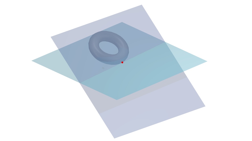
Figure 4: (Color online.) A schematic illustration of the topological reason why the value of a multivariate residue is not uniquely determined by the pole enclosed by the integration cycle, but also depends on the cycle. The figure is a projection of the two-complex-dimensional (i.e., four-real-dimensional) situation for the differential form $\omega$ in eq. (9). The planes represent the divisors of $\omega$. For visual clarity only two planes are shown. The red dot represents the pole $p=(0,0)$, and the tori two distinct integration cycles enclosing the pole. Because of the presence of the divisors, the cycle in the left figure cannot be continuously deformed into the one in the right figure: the cycles are non-homologous. As a result, the contours are not guaranteed to produce equal residues, and in general they will not. It is an artifact of the two-dimensional projection of the four-dimensional situation that the torus in the right figure appears to intersect the divisors and not to enclose the pole.

We can apply the residue evaluation algorithm of section 2.1 to each of the two terms in eq. (110) separately, yielding $R_{1}$ and $R_{2}$ for the first and second term, respectively. (Recall eqs. (17)–(18) for the expressions for $R_{1}$ and $R_{2}$.) Combining this with the observations made in the discussion below eq. (119), we see that in the region $M^{+++}$ of the moduli space, the residue evaluates to $0$; in $M^{+--}$ to $R_{1}$; in $M^{+-+}$ to $R_{2}$; and in $M^{++-}$ to $R_{1}+R_{2}=-R_{3}$ (cf. eq. (20)). From these observations we conclude that we have the following one-to-one map between the partitionings of the denominator of $\omega$ in eq. (11) and the regions of the moduli space of integration cycles,

$$\{\varphi_{1},\varphi_{2}\varphi_{3}\} \longleftrightarrow\hskip 5.69054ptM^{+--}$$ (121)

$$\{\varphi_{2},\varphi_{3}\varphi_{1}\} \longleftrightarrow\hskip 5.69054ptM^{+-+}$$

$$\{\varphi_{3},\varphi_{1}\varphi_{2}\} \longleftrightarrow\hskip 5.69054ptM^{++-}\,.$$

This map provides a dictionary between the algebraic and geometric pictures of the distinct residues defined at the given pole.

We remark that the relation (20) shows that only two of the regions $M^{+--},M^{+-+},\ldots$ define linearly independent integration cycles.

References

- [1] F. Cachazo, D. Skinner, On the structure of scattering amplitudes in super Yang-Mills and supergravity, (2008). arXiv:0801.4574.
- [2] F. Cachazo, Sharpening The Leading Singularity, (2008). arXiv:0803.1988.
- [3] D. A. Kosower, K. J. Larsen, Maximal Unitarity at Two Loops, Phys. Rev. D85 (2012) 045017. arXiv:1108.1180.
- [4] S. Caron-Huot, K. J. Larsen, Uniqueness of two-loop master contours, JHEP 10 (2012) 026. arXiv:1205.0801.
- [5] M. Søgaard, Y. Zhang, Multivariate Residues and Maximal Unitarity, JHEP 12 (2013) 008. arXiv:1310.6006.
- [6] H. Johansson, D. A. Kosower, K. J. Larsen, M. Søgaard, Cross-Order Integral Relations from Maximal Cuts, Phys. Rev. D92 (2) (2015) 025015. arXiv:1503.06711.
- [7] N. Arkani-Hamed, F. Cachazo, C. Cheung, J. Kaplan, A Duality For The S Matrix, JHEP 03 (2010) 020. arXiv:0907.5418.
- [8] N. Arkani-Hamed, J. Bourjaily, F. Cachazo, J. Trnka, Unification of Residues and Grassmannian Dualities, JHEP 01 (2011) 049. arXiv:0912.4912.
- [9] N. Arkani-Hamed, J. L. Bourjaily, F. Cachazo, J. Trnka, Local Integrals for Planar Scattering Amplitudes, JHEP 06 (2012) 125. arXiv:1012.6032.
- [10] N. Arkani-Hamed, J. L. Bourjaily, F. Cachazo, A. B. Goncharov, A. Postnikov, J. Trnka, Scattering Amplitudes and the Positive Grassmannian, Cambridge University Press. ISBN 9781107086586. arXiv:1212.5605.
- [11] N. Arkani-Hamed, J. Trnka, Into the Amplituhedron, JHEP 12 (2014) 182. arXiv:1312.7878.
- [12] N. Arkani-Hamed, J. L. Bourjaily, F. Cachazo, A. Postnikov, J. Trnka, On-Shell Structures of MHV Amplitudes Beyond the Planar Limit, JHEP 06 (2015) 179. arXiv:1412.8475.
- [13] N. Arkani-Hamed, A. Hodges, J. Trnka, Positive Amplitudes In The Amplituhedron, JHEP 08 (2015) 030. arXiv:1412.8478.
- [14] Z. Bern, E. Herrmann, S. Litsey, J. Stankowicz, J. Trnka, Evidence for a Nonplanar Amplituhedron, JHEP 06 (2016) 098. arXiv:1512.08591.
- [15] E. Herrmann, J. Trnka, Gravity On-shell Diagrams, JHEP 11 (2016) 136. arXiv:1604.03479.
- [16] G. Chen, T. Wang, BCJ Numerators from Differential Operator of Multidimensional Residue (2017). arXiv:1709.08503.
- [17] Z. Bern, J. J. M. Carrasco, H. Johansson, New Relations for Gauge-Theory Amplitudes, Phys. Rev. D78 (2008) 085011. arXiv:0805.3993, doi:10.1103/PhysRevD.78.085011.
- [18] Z. Bern, J. J. M. Carrasco, H. Johansson, Perturbative Quantum Gravity as a Double Copy of Gauge Theory, Phys. Rev. Lett. 105 (2010) 061602. arXiv:1004.0476, doi:10.1103/PhysRevLett.105.061602.
- [19] Eduardo Cattani and Alicia Dickenstein, Solving Polynomial Equations, Chapter 1: Introduction to residues and resultants, Springer Berlin Heidelberg, 2005. ISBN 978-3-540-24326-7. (Also available online at http://people.math.umass.edu/cattani/chapter1.pdf).
- [20] S. Poslavsky, Rings: an efficient Java/Scala library for polynomial rings, Comput. Phys. Commun. 235 (2019) 400–413. arXiv:1712.02329, doi:10.1016/j.cpc.2018.09.005.
- [21] Phillip Griffiths and Joseph Harris, Principles of Algebraic Geometry, John Wiley & Sons, 1978. ISBN 0-471-32792-1.
-
[22]
D. Lichtblau, Practical computations with Gröbner bases,
https://www.researchgate.net/publication/
260165637_Practical_computations_with_Grobner_bases. - [23] David A. Cox, John Little, Donal O’Shea, Using Algebraic Geometry (second edition), Springer Berlin Heidelberg, 2006. ISBN 978-0-387-27105-7.
- [24] David A. Cox, John Little, Donal O’Shea, Ideals, Varieties, and Algorithms (third edition), Springer Berlin Heidelberg, 2006. ISBN 978-3-319-16721-3.
- [25] S. Weinzierl, The Art of computing loop integrals, in: Universality and renormalization: From stochastic evolution to renormalization of quantum fields. Proceedings, Workshop on ’Percolation, SLE and related topics’, Toronto, Canada, September 20-24, 2005, and Workshop on ’Renormalization and universality in mathematical physics’, Toronto, Canada, October 18-22, 2005, 2006, pp. 345–395. arXiv:hep-ph/0604068.
- [26] Z. Bern, L. J. Dixon, D. A. Kosower, On-Shell Methods in Perturbative QCD, Annals Phys. 322 (2007) 1587–1634. arXiv:0704.2798, doi:10.1016/j.aop.2007.04.014.
- [27] R. K. Ellis, Z. Kunszt, K. Melnikov, G. Zanderighi, One-loop calculations in quantum field theory: from Feynman diagrams to unitarity cuts, Phys. Rept. 518 (2012) 141–250. arXiv:1105.4319, doi:10.1016/j.physrep.2012.01.008.
- [28] Z. Bern, L. J. Dixon, D. C. Dunbar, D. A. Kosower, Fusing gauge theory tree amplitudes into loop amplitudes, Nucl. Phys. B435 (1995) 59–101. arXiv:hep-ph/9409265, doi:10.1016/0550-3213(94)00488-Z.
- [29] R. Britto, F. Cachazo, B. Feng, Generalized unitarity and one-loop amplitudes in super-Yang-Mills, Nucl. Phys. B725 (2005) 275–305. arXiv:hep-th/0412103.
- [30] F. Cachazo, S. He, E. Y. Yuan, Scattering of Massless Particles in Arbitrary Dimensions, Phys. Rev. Lett. 113 (17) (2014) 171601. arXiv:1307.2199, doi:10.1103/PhysRevLett.113.171601.
- [31] M. Søgaard, Y. Zhang, Scattering Equations and Global Duality of Residues, Phys. Rev. D93 (10) (2016) 105009. arXiv:1509.08897, doi:10.1103/PhysRevD.93.105009.
- [32] J. Bosma, M. Søgaard, Y. Zhang, The Polynomial Form of the Scattering Equations is an H-Basis, Phys. Rev. D94 (4) (2016) 041701. arXiv:1605.08431, doi:10.1103/PhysRevD.94.041701.
-
[33]
Kasper J. Larsen and Robbert Rietkerk, MultivariateResidues,
https://bitbucket.org/kjlarsen/multivariateresidues/raw
/master/release/MultivariateResidues.zip (2018).