Online Learning Sensing Matrix and Sparsifying Dictionary Simultaneously
for Compressive Sensing

Abstract

This paper considers the problem of simultaneously learning the Sensing Matrix and Sparsifying Dictionary (SMSD) on a large training dataset. To address the formulated joint learning problem, we propose an online algorithm that consists of a closed-form solution for optimizing the sensing matrix with a fixed sparsifying dictionary and a stochastic method for learning the sparsifying dictionary on a large dataset when the sensing matrix is given. Benefiting from training on a large dataset, the obtained compressive sensing (CS) system by the proposed algorithm yields a much better performance in terms of signal recovery accuracy than the existing ones. The simulation results on natural images demonstrate the effectiveness of the suggested online algorithm compared with the existing methods.

1 Introduction

Sparse representation (Sparseland) has led to numerous successful applications spanning through many fields, including image processing, machine learning, pattern recognition, and compressive sensing (CS) [1] - [6]. This model assumes that a signal $\bm{x}\in\Re^{N}$ can be represented as a linear combination of a few columns, also known as atoms, taken from a matrix $\bm{\Psi}\in\Re^{N\times L}$ (referred to as a dictionary):

$$\bm{x}=\bm{\Psi}\bm{\theta}+\bm{e},$$ (1)

where $\bm{\theta}\in\Re^{L}$ has few non-zero entries and is the representation coefficient vector of $\bm{x}$ over the dictionary $\bm{\Psi}$ and $\bm{e}\in\Re^{N}$ is known as the sparse representation error (SRE) which is not nil in general case. The signal $\bm{x}$ is called $K$-sparse in $\bm{\Psi}$ if $\|\bm{\theta}\|_{0}\leq K$ where $\|\bm{\theta}\|_{0}$ is used to count the number of non-zeros in $\bm{\theta}$.

The choice of dictionary $\bm{\Psi}$ depends on specific applications and can be a predefined one, e.g., discrete cosine transform (DCT), wavelet transform and a multiband modulated discrete prolate spheroidal sequences (DPSS’s) dictionary [7] etc. It is also beneficial and recently widely-utilized to adaptively learn a dictionary $\bm{\Psi}$, called dictionary learning, such that a set of $P$ training signals $\{\bm{x}_{k},k=1,2,\cdots,P\}$ is sparsely represented by optimizing a $\bm{\Psi}$. There exist many efficient algorithms to learn a dictionary [3] and the most two popular methods among them are the method of optimal directions (MOD) [4] and the K-singular value decomposition (KSVD) algorithm [5]. In particular, we prefer to use an over-complete dictionary [5], $N<L$.

CS is an emerging framework that enables to exactly recover the signal $\bm{x}$, in which it is sparse or sparsely represented by a dictionary $\bm{\Psi}$, from a number of linear measurements that is considerably lower than the size of samples required by the Shannon-Nyquist theorem [6]. Generally speaking, researchers tend to utilize a random matrix $\bm{\Phi}\in\Re^{M\times N}$ as the sensing matrix (a.k.a projection matrix) to obtain the linear measurements

$$\bm{y}=\bm{\Phi}\bm{x}=\bm{\Phi}\bm{\Psi}\bm{\theta}+\bm{\Phi}\bm{e},$$ (2)

where $M\ll N$. Abundant efforts have been devoted to optimize the sensing matrix with a predefined dictionary resulting in a CS system that outperforms the standard one (random matrix) in various cases [8] - [15].

Recently, researchers realize simultaneously optimizing sensing matrix and dictionary for the CS system yields a higher signal reconstruction accuracy than the classical CS systems which only optimize sensing matrix with a fixed dictionary [14, 15]. The main idea underlying in [14, 15] is to consider the influence of SRE in learning the dictionary (see Section 3 for the formal problem). Alternating minimization methods are introduced to jointly design the sensing matrix $\bm{\Phi}$ and the dictionary $\bm{\Psi}$ in [14, 15]. Compared to [14], closed-form solutions for updating the sensing matrix and the dictionary are derived in [15] which hence obtains a better performance in terms of signal recovery accuracy. The disadvantage of the method in [15] is that it involves many singular value decompositions (SVDs) making their algorithm inefficient in practice.

Although the method for jointly optimizing the sensing matrix and the dictionary in [14, 15] works well for a small-scale training dataset (e.g., $N=64$ and $P=10^{4}$), it becomes inefficient (and even impractical) if the dimension of the dictionary is high or the size of training dataset is very large (say with more than $10^{6}$ patches in natural images situation) or for the case involving dynamic data like video stream. It is easy to see that the methods in [14, 15] require heavy memory and computations to address such a large scale optimization problem because they have to sweep all of the training data in each dictionary updating procedure. Inspired by [18, 19], an online algorithm with less complexity and memory is introduced to address the same learning problem shown in [14, 15] but on a large dataset. We use a toy example to briefly explain the benefit of training on a large-scale dataset. Assume that the dimension of the dictionary is $64\times 100$ and the number of non-zeros in the sparse vector $\bm{\theta}$ is $4$. Then the number of subspaces in this dictionary attains $\binom{100}{4}\approx 3.9\times 10^{6}$. Thus, we see such a dictionary provides a rich number of subspaces which motives us to train the dictionary on a large-scale dataset to explore the dictionary to represent the signal of interests better. One can still imagine that along with the increase of the dimension of the dictionary, the number of subspaces will become much richer and we can expect such a dictionary may yield many interesting properties. Indeed, the benefit of learning a dictionary on a large dataset or a high dimension (without training the sensing matrix) has been experimentally demonstrated in [25, 26, 29]. Moreover, the simulations shown in this paper also indicate the merit of learning the CS system (both the dictionary and the sensing matrix) on a large-scale dataset.

Note that, in each step, the sensing matrix is either updated with an iterative algorithm in [14] or an alternating-minimization method in [15], both requiring many times of SVDs. To overcome this issue, we suggest an efficient method to optimize the sensing matrix which is robust to the SRE. The proposed method is inspired by the recent results in [10, 11, 13] for robust sensing matrices, but it differs from these works in which there is no need to tune the trade-off parameter and hence it is more suitable for online learning and dynamic data. The experiments on natural images demonstrate that jointly optimizing the Sensing Matrix and Sparsifying Dictionary (SMSD) on a large dataset has much better performance in terms of signal recovery accuracy than with the ones shown in [14, 15]. Notice that in this paper we want to design a CS system for the applications where the SRE exists in which is the case for the natural images.

The rest of this paper is organized as follows. In Section 2, a novel model is proposed to design the sensing matrix to reduce the coherence between each two columns in $\bm{\Phi}\bm{\Psi}$ and overcome the influence of SRE. Moreover, a closed-form solution is derived to obtain the optimized sensing matrix which is parameter free and then more suitable for the following joint learning SMSD method. A joint optimization algorithm for learning SMSD on a large dataset is suggested in Section 3. For learning the sparsifying dictionary on a large dataset efficiently, an online method is introduced to consider such a large training data. Some experiments on natural images are carried out in Section 4 to demonstrate the effectiveness of the proposed algorithm and the advantage of training on a large dataset comparing with other methods. Conclusion and future work are given in Section 5.

2 An Efficient Method for Robust Sensing Matrix Design

In this section, we present an efficient method to design a robust sensing matrix. To begin, we note that one of the major purposes in optimizing the sensing matrix is to reduce the coherence between each two columns of the equivalent dictionary $\bm{\Phi}\bm{\Psi}$. This leads to the work [8, 9] which demonstrates that the optimized sensing matrix such that the equivalent dictionary with small mutual coherence yields much better performance than the one with a random sensing matrix for the exactly sparse signals (i.e., $\bm{e}=\bm{0}$ for the signal model (1)). See also [20, 21] for directly minimizing the mutual coherence of the equivalent dictionary. However, it was recently realized [10, 11, 13] that such a sensing matrix is not robust to SRE and thus the corresponding CS system results in poor performance in practice, like sampling the natural images, where the SRE exists even when we represent the images with a well designed dictionary. Alternatively, the average mutual coherence (i.e., the coherence on a least square metric instead of the infinity norm) rather than the exact mutual coherence is suggested in [10, 11] for designing an optimal robust sensing matrix. Specifically, a robust sensing matrix is attained by solving [10, 11]:

$$\min_{\bm{\Phi}}\leavevmode\nobreak\ \|\bm{I}_{L}-\bm{\Psi}^{\mathcal{T}}\bm{\Phi}^{\mathcal{T}}\bm{\Phi}\bm{\Psi}\|_{F}^{2}+\lambda\|\bm{\Phi}\bm{E}\|_{F}^{2}$$ (3)

where $\|\cdot\|_{F}$ denotes the Frobenius norm and $\bm{I}_{L}$ represents an identity matrix with dimension $L$. According to the recent result shown in [13], it suggests replacing the penalty $\|\bm{\Phi}\bm{E}\|_{F}^{2}$ by $\|\bm{\Phi}\|_{F}^{2}$ (which is independent of the training data) since $\|\bm{\Phi}\|_{F}^{2}$ has the same effectiveness as $\|\bm{\Phi}\bm{E}\|_{F}^{2}$ when the SRE is modelled as the Gaussian noise and $P\rightarrow\infty$. Thus, the robust sensing matrix is developed via addressing [13]:

$$\min_{\bm{\Phi}}\leavevmode\nobreak\ f(\bm{\Phi})=\|\bm{I}_{L}-\bm{\Psi}^{\mathcal{T}}\bm{\Phi}^{\mathcal{T}}\bm{\Phi}\bm{\Psi}\|_{F}^{2}+\lambda\|\bm{\Phi}\|_{F}^{2}$$ (4)

Numerical experiments with natural images show that the optimized sensing matrix through solving (4) with a well-chosen $\lambda$ yields state-of-the-art performance in CS-based image compression [13]. However, we note that it is nontrivial to choose an optimal $\lambda$ for (4) since the two terms $\|\bm{I}_{L}-\bm{\Psi}^{\mathcal{T}}\bm{\Phi}^{\mathcal{T}}\bm{\Phi}\bm{\Psi}\|_{F}^{2}$ and $\|\bm{\Phi}\|_{F}^{2}$ have different physical meanings: the formal represents the average mutual coherence of the equivalent dictionary $\bm{\Phi}\bm{\Psi}$, while the later is the energy of the sensing matrix $\bm{\Phi}$. For off-line applications when the dictionary is fixed, it is suggested to choose a $\lambda$ by searching a given range and looking at the performance of the resulted sensing matrices [10, 11, 13] on the testing dataset. However, this strategy becomes very inefficient for online applications when the dictionary $\bm{\Psi}$ is evolving which belongs to the case in this paper. To avoid tuning the parameter $\lambda$, we suggest designing the robust sensing matrix with the following two steps: find a set of solutions which minimize $\|\bm{I}_{L}-\bm{\Psi}^{\mathcal{T}}\bm{\Phi}^{\mathcal{T}}\bm{\Phi}\bm{\Psi}\|_{F}^{2}$ (i.e., solve (4) without the term $\|\bm{\Phi}\|_{F}^{2}$), and then locate a $\bm{\Phi}$ among these solutions that has smallest energy. Thus, we consider the following optimization problem to design the sensing matrix which is slightly different from (4):

$$\left.\begin{array}[]{rl}\min\limits_{\bm{\Phi}\in\mathcal{S}}&\|\bm{\Phi}\|_{F}^{2}\\ {\mathcal{S}=}&\arg\min\limits_{\tilde{\bm{\Phi}}\in\Re^{M\times N}}\leavevmode\nobreak\ \leavevmode\nobreak\ g(\tilde{\bm{\Phi}})=\|\bm{I}_{L}-\bm{\Psi}^{\mathcal{T}}\tilde{\bm{\Phi}}^{\mathcal{T}}\tilde{\bm{\Phi}}\bm{\Psi}\|_{F}^{2}\end{array}\right.$$ (5)

Let ${\mathcal{U}}_{M,\bar{N}}:=\left\{\bm{U}_{M,\bar{N}}:\bm{U}_{M,\bar{N}}^{\cal T}\bm{U}_{M,\bar{N}}=\bm{I}_{\bar{N}}\right\}$ denote the set of $M\times\bar{N}$ orthonormal matrices for $\bar{N}\leq M$. When $\bar{N}=M$, to simplify the notation, we use $\mathcal{U}_{M}$ to denote the set of $M\times M$ orthonormal matrices. The following result establishes a set of closed-form solutions for (5):

Theorem 1.

Let $\bm{\Psi}=\bm{U}_{\bm{\Psi}}\bm{\Lambda}\bm{V}_{\bm{\Psi}}^{\mathcal{T}}$ be an SVD of $\bm{\Psi}$, where $\text{Rank}(\bm{\Psi})=\bar{N}\leq N$, $\bm{\Lambda}=\text{diag}(\lambda_{1},\lambda_{2},\cdots,\lambda_{\bar{N}})>0$ with $\lambda_{1}\geq\lambda_{2}\geq\cdots\geq\lambda_{\bar{N}}$, and $\bm{U}_{\bm{\Psi}}$ and $\bm{V}_{\bm{\Psi}}$ are $N\times\bar{N}$ and $L\times\bar{N}$ orthonormal matrices, respectively. When $\bar{N}\geq M$, a set of optimal solutions for (5) is specified by

$${\cal W}_{1}:=\left\{\bm{\Phi}:\bm{\Phi}=\begin{bmatrix}\bm{U}_{M}&\bm{0}\end{bmatrix}\bm{\Lambda}^{-1}\bm{U}_{\bm{\Psi}}^{\mathcal{T}},\bm{U}_{M}\in{\cal U}_{M}\right\}$$ (6)

On the other hand, when $\bar{N}<M$, a set of optimal solutions for (5) is specified by

$${\cal W}_{2}:=\left\{\bm{\Phi}:\bm{\Phi}=\bm{U}_{M,\bar{N}}\bm{\Lambda}^{-1}\bm{U}_{\bm{\Psi}}^{\mathcal{T}},\bm{U}_{M,\bar{N}}\in\mathcal{U}_{M\times\bar{N}}\right\}$$ (7)

Proof.

We first rewrite $g({\bm{\Phi}})$ as

$$g(\bm{\Phi}) =\|\bm{I}_{L}-\bm{V}_{\bm{\Psi}}\bm{\Lambda}\bm{U}_{\bm{\Psi}}^{\mathcal{T}}\bm{\Phi}^{\mathcal{T}}\bm{\Phi}\bm{U}_{\bm{\Psi}}\bm{\Lambda}\bm{V}_{\bm{\Psi}}^{\mathcal{T}}\|_{F}^{2}$$

$$=\|\bm{I}_{\bar{N}}-\bm{\Lambda}\bm{U}_{\bm{\Psi}}^{\mathcal{T}}\bm{\Phi}^{\mathcal{T}}\bm{\Phi}\bm{U}_{\bm{\Psi}}\bm{\Lambda}\|_{F}^{2}+L-\bar{N}$$

Thus, minimizing $g(\bm{\Phi})$ is equivalent to

$$\min_{\bm{\Phi}}h(\bm{\Phi})=\|\bm{I}_{\bar{N}}-\bm{\Lambda}\bm{U}_{\bm{\Psi}}^{\mathcal{T}}\bm{\Phi}^{\mathcal{T}}\bm{\Phi}\bm{U}_{\bm{\Psi}}\bm{\Lambda}\|_{F}^{2}.$$ (8)

We proceed by considering the following two cases.

case I: $\bar{N}\geq M$. Noting that $\text{rank}(\bm{\Lambda}\bm{U}_{\bm{\Psi}}^{\mathcal{T}}\bm{\Phi}^{\mathcal{T}}\bm{\Phi}\bm{U}_{\bm{\Psi}}\bm{\Lambda})=M\leq\bar{N}$ and utilizing the Eckart-Young-Mirsky theorem [22], we have that $h(\bm{\Phi})\geq\bar{N}-M$ and it achieves its minimum when

$$\bm{\Lambda}\bm{U}_{\bm{\Psi}}^{\mathcal{T}}\bm{\Phi}^{\mathcal{T}}\bm{\Phi}\bm{U}_{\bm{\Psi}}\bm{\Lambda}=\bm{U}_{\bar{N},M}\bm{U}_{\bar{N},M}^{\cal T},$$

where $\bm{U}_{\bar{N},M}$ is an arbitrary $\bar{N}\times M$ orthonormal matrix. The set of $\bm{\Phi}$ that satisfies the above equation is given by

$$\bm{\Phi}\in\mathcal{S}=\left\{\bm{U}_{\bar{N},M}^{\cal T}\bm{\Lambda}^{-1}\bm{U}_{\bm{\Psi}}^{\mathcal{T}}:\bm{U}_{\bar{N},M}^{\cal T}\bm{U}_{\bar{N},M}=\bm{I}_{M}\right\}.$$ (9)

With this, we turn to find $\bm{\Phi}$ such that it has the smallest $\|\bm{\Phi}\|_{F}^{2}$. To that end, we rewrite

$$\|\bm{\Phi}\|_{F}^{2}=\text{Tr}\left(\bm{\Phi}^{\mathcal{T}}\bm{\Phi}\right)=\text{Tr}\left(\bm{U}_{\bar{N},M}\bm{U}_{\bar{N},M}^{\cal T}\bm{\Lambda}^{-2}\right)=\sum_{i=1}^{\bar{N}}\frac{\alpha_{i}}{\lambda_{i}^{2}}\\$$

where $\alpha_{i}$ is the $i$-th diagonal of $\bm{U}_{\bar{N},M}\bm{U}_{\bar{N},M}^{\cal T}$. It is clear that $0\leq\alpha_{i}\leq 1$ and $\sum_{i=1}^{\bar{N}}\alpha_{i}=M$ since $\bm{U}_{\bar{N},M}$ is an $\bar{N}\times M$ orthonormal matrix. Therefore, we have $\sum_{i=1}^{\bar{N}}\frac{\alpha_{i}}{\lambda_{i}^{2}}\geq\sum_{i=1}^{M}\frac{1}{\lambda_{i}^{2}}$ and it achieves the minimum value when $\alpha_{1}=\cdots=\alpha_{M}=1$ and $\alpha_{M+1}=\cdots=\alpha_{\bar{N}}=0$. The last condition implies that $\bm{U}_{\bar{N},M}=\begin{bmatrix}\bm{U}_{M}\\ \bm{0}\end{bmatrix}$ with $\bm{U}_{M}$ is an arbitrary $M\times M$ orthonormal matrix.

case II: $\bar{N}<M$. We first note that $h(\bm{\Phi})\geq 0$ and it achieves its minimum when

$$\bm{\Phi}\in\mathcal{S}=\left\{\bm{U}_{M,\bar{N}}\bm{\Lambda}^{-1}\bm{U}_{\bm{\Psi}}^{\mathcal{T}}:\bm{U}_{M,\bar{N}}^{\cal T}\bm{U}_{\bar{N},M}=\bm{I}_{\bar{N}}\right\}.$$

where $\bm{U}_{M,\bar{N}}$ is an arbitrary $M\times\bar{N}$ orthonormal matrix. For such $\bm{\Phi}$, we have

$$\|\bm{\Phi}\|_{F}^{2}=\text{Tr}\left(\bm{\Phi}^{\mathcal{T}}\bm{\Phi}\right)=\text{Tr}\left(\bm{\Lambda}^{-2}\right)=\sum_{i=1}^{\bar{N}}\frac{1}{\lambda_{i}^{2}}$$

which implies that each $\bm{\Phi}$ has the same energy. ∎

We remark that [9, Theorem 2] also gives the set of optimal solutions that minimizes $g(\bm{\Phi})$ for the case $\text{Rank}(\bm{\Psi})=\bar{N}\geq M$, i.e., $\overline{\cal S}=\left\{\begin{bmatrix}\bm{U}_{M}&\bm{0}\end{bmatrix}\bm{\Lambda}^{-1}\bm{U}_{\bm{\Psi}}^{\mathcal{T}},\bm{U}_{M}\in{\cal U}_{M}\right\}.$ By noting that $\begin{bmatrix}\bm{U}_{M}^{\mathcal{T}}\\ \bm{0}\end{bmatrix}\in{\cal U}_{\bar{N},M}$, it is clear that ${\cal S}=\overline{\cal S}$ where $\cal S$ is given in (9).

When $\text{Rank}(\bm{\Psi})=\bar{N}\geq M$ (which is true for most of applications), (6) gives a set of optimal solutions for (5) and implies that there exists some degrees of freedom to choosing $\bm{U}_{M}$. The following result investigates the performance of the sensing matrices with different $\bm{U}_{M}$.

Lemma 1.

Compressive sensing systems with the same dictionary $\bm{\Psi}$ and different $\bm{\Phi}\in\mathcal{W}_{1}$ (which is defined in (6)) have the same performance.

Proof.

Suppose we have two compressive sensing systems with the same dictionary $\bm{\Psi}$ and the sensing matrices $\bm{\Phi}=\begin{bmatrix}\bm{U}_{M}&\bm{0}\end{bmatrix}\bm{\Lambda}^{-1}\bm{U}_{\bm{\Psi}}^{\mathcal{T}}$ and $\overline{\bm{\Phi}}=\begin{bmatrix}\overline{\bm{U}}_{M}&\bm{0}\end{bmatrix}\bm{\Lambda}^{-1}\bm{U}_{\bm{\Psi}}^{\mathcal{T}}$, respectively, where $\bm{U}_{M},\overline{\bm{U}}_{M}\in{\cal U}_{M}$. For any $\bm{x}\in\Re^{N}$, the two CS systems obtain the measurements as $\bm{y}=\bm{\Phi}\bm{x},\ \overline{\bm{y}}=\overline{\bm{\Phi}}\bm{x}$ and respectively attempt to recover $\bm{x}$ via

$$\min_{\theta}\|\bm{y}-\bm{\Phi}\bm{\Psi}\bm{\theta}\|^{2},\leavevmode\nobreak\ \leavevmode\nobreak\ \text{s.t.}\leavevmode\nobreak\ \leavevmode\nobreak\ \|\bm{\theta}\|_{0}\leq K$$

and

$$\min_{\theta}\|\overline{\bm{y}}-\overline{\bm{\Phi}}\bm{\Psi}\bm{\theta}\|^{2},\leavevmode\nobreak\ \leavevmode\nobreak\ \text{s.t.}\leavevmode\nobreak\ \leavevmode\nobreak\ \|\bm{\theta}\|_{0}\leq K$$

The proof is completed by noting that the above two equations have the same solution since

$$\|\bm{y}-\bm{\Phi}\bm{\Psi}\bm{\theta}\|^{2}=\|\overline{\bm{U}}_{M}\bm{U}_{M}^{\cal T}\left(\bm{y}-\bm{\Phi}\bm{\Psi}\bm{\theta}\right)\|^{2}=\|\overline{\bm{y}}-\overline{\bm{\Phi}}\bm{\Psi}\bm{\theta}\|^{2}$$

∎

Lemma 1 implies that we can choose a $\bm{\Phi}$ in (6) with $\bm{U}_{M}$ as an identity matrix and it has the same performance as other $\bm{\Phi}\in{\cal W}_{1}$. Moreover, by choosing an identity matrix for $\bm{U}_{M}$, we can save computations in learning the dictionary and the solution for (5) becomes

$$\bm{\Phi}=\phi(\bm{\Psi})\triangleq\bm{\Lambda}_{M}^{-1}\bm{U}_{\bm{\Psi}}\left(:,1:M\right)^{\mathcal{T}}$$ (10)

where $\bm{\Lambda}_{M}=\bm{\Lambda}(1:M,1:M)$. Clearly, $\bm{\Lambda}_{M}$ is a diagonal matrix and the calculation of its inverse is cheap. In effect, one time SVD of the dictionary $\bm{\Psi}$ dominates the main complexity in the sensing matrix updating procedure. Compared with the methods shown in [14, 15] which need to perform the eigenvalue decomposition or SVD many times, our proposed method already saves significant computations.

We end this section by comparing (10) with gradient descent solving (4) in terms of the computational complexity, though we note that our main purpose to use (10) is to avoid tuning the parameter $\lambda$ in (4). The gradient of $f(\bm{\Phi})$ is given as follows

$$\nabla_{\bm{\Phi}}f(\bm{\Phi})=2\lambda\bm{\Phi}-4\bm{\Phi}\bm{\Psi}\bm{\Psi}^{\mathcal{T}}+4\bm{\Phi}\bm{\Psi}\bm{\Psi}^{\mathcal{T}}\bm{\Phi}^{\mathcal{T}}\bm{\Phi}\bm{\Psi}\bm{\Psi}^{\mathcal{T}}.$$

Suppose $\bm{\Psi}\bm{\Psi}^{\mathcal{T}}$ is precomputed and then evaluating the gradient $\nabla_{\bm{\Phi}}f(\bm{\Phi})$ requires $O(MN^{2})$ computations. Thus, the gradient descent has at least $O(MN^{2})$ computational complexity, though we are not ensured how fast the gradient descent converges. As indicated by (9), our closed-form solution only needs to compute the first $M$ eigenvectors and corresponding eigenvalues of $\bm{\Psi}\bm{\Psi}^{T}$, which has computational complexity of $O(MN^{2})$. We also note that in the dictionary updating procedure (see (18) in Section 3), it is required to compute $(\bm{I}_{N}+\frac{1}{\gamma}\bm{\Phi}^{\mathcal{T}}\bm{\Phi})^{-1}$, which can be directly obtained through (10) (the SVD form of $\bm{\Psi}$). If we utilize the gradient descent method to update $\bm{\Phi}$, then we still need to compute such an inverse when updating the dictionary and this can be saved if we utilize (10).

3 Online Learning SMSD Simultaneously

We begin this section by considering the problem of jointly optimizing the SMSD on a very large training dataset first. Moreover, the corresponding joint optimization problem is solved via the alternating-minimization based approach. In order to reduce the complexity of learning a dictionary on such a large training data, an online algorithm with the consideration of the influence of the projected SRE, i.e., $\|\bm{\Phi}\bm{e}\|_{2}$, is developed.

3.1 Online Joint SMSD Optimization

Given a set of $P$ training signals $\bm{X}(:,k)=\bm{x}_{k}$, $k=1,2,\cdots,P$, our purpose here is to jointly design the SMSD. To this end, a proper framework is required. Classical dictionary learning attempts to minimize the following sparse representation error (SRE):

$$\min\limits_{\bm{\Psi}\in\mathcal{C},\bm{\Theta}}\|\bm{X}-\bm{\Psi}\bm{\Theta}\|_{F}^{2},\leavevmode\nobreak\ \leavevmode\nobreak\ \text{s.t.}\leavevmode\nobreak\ \leavevmode\nobreak\ \|\bm{\theta}_{k}\|_{0}\leq K,\leavevmode\nobreak\ \forall k$$ (11)

where $\bm{\Theta}(:,k)=\bm{\theta}_{k}$, $\forall k$ contains the sparse coefficient vectors and $\mathcal{C}$ is a constraint set to avoid trivial solutions.

Note that in CS, we obtain the linear measurements $\bm{y}$ as in (2) and then recover the signal from $\bm{y}$ by first recovering the sparse coefficients $\bm{\theta}$ and then obtain $\bm{x}$ via $\bm{\Psi}\bm{\theta}$. Therefore, a smaller $\bm{\Phi}\bm{e}$ is also preferred. This implies that besides reducing the SRE $\|\bm{X}-\bm{\Psi}\bm{\Theta}\|_{F}^{2}$, giving a sensing matrix $\bm{\Phi}$, the dictionary is also expected to reduce the projected SRE $\|\bm{\Phi}(\bm{X}-\bm{\Psi}\bm{\Theta})\|_{F}^{2}$ [14]-[17]. Now the sensing matrix and the sparsifying dictionary are jointly optimized by [14, 15]

$$\begin{array}[]{rl}\min\limits_{\bm{\Psi}\in\mathcal{C},\bm{\Theta},\bm{\Phi}}&\gamma\|\bm{X}-\bm{\Psi}\bm{\Theta}\|_{F}^{2}+\|{\bm{\Phi}\bm{X}}-\bm{\Phi}\bm{\Psi}\bm{\Theta}\|_{F}^{2}\\ \text{s.t.}&\bm{\Phi}=\phi(\bm{\Psi}),\|\bm{\theta}_{k}\|_{0}\leq K,\leavevmode\nobreak\ \forall k\end{array}$$ (12)

where $\phi(\bm{\Psi})$ is given in (10) and $\gamma\in\left[0,1\right]$ is a trade-off parameter to balance the SRE and the projected SRE. The value of $\gamma$ can be determined through grid search to receive the highest signal recovery accuracy on the testing dataset.

Remark 3.1:

• We first note that the projected SRE $\|\bm{\Phi}(\bm{X}-\bm{\Psi}\bm{\Theta})\|_{F}^{2}$ also involves the sensing matrix $\bm{\Phi}$ and hence this term should also be considered in designing the sensing matrix. As we explained in Section 2, the sensing matrix $\phi(\bm{\Psi})$ given in (10) already incorporates the projected SRE. This suggests the advantages of our proposed method for designing the sensing matrix compared with the ones utilized in [14, 15] where the projected SRE is not considered.

• Compared with a separate approach that (usually) first learns the dictionary by (11) and then designs the sensing matrix with the learned dictionary, jointly learning the SMSD via (12) is expected to yield a better CS system as the projected SRE is also minimized sequentially. We refer [14, 15] for more discussions regarding the advantages of this joint approach.

Similar to [14, 15], we utilize the alternating-minimization based method for solving the above joint optimization problem (12). The main idea is to alternatively update the sensing matrix (when the dictionary and sparse coefficients are fixed) by (10) which is cheap and update the dictionary and the sparse coefficients by minimizing the objective function in (12) when the sensing matrix is fixed, i.e.,

$$\begin{array}[]{rl}\min\limits_{\bm{\Psi}\in\mathcal{C},\bm{\Theta}}&\sigma(\bm{\Psi},\bm{\Theta})\triangleq\gamma\|\bm{X}-\bm{\Psi}\bm{\Theta}\|_{F}^{2}+\|\bm{Y}-\bm{\Phi}\bm{\Psi}\bm{\Theta}\|_{F}^{2}\\ \text{s.t.}&\|\bm{\theta}_{k}\|_{0}\leq K,\leavevmode\nobreak\ \forall k\end{array}$$ (13)

where $\bm{Y}=\bm{\Phi}\bm{X}$. As we suggest utilizing a large training dataset to learn the dictionary, an online algorithm is proposed in next subsection to fit such a large-scale case. We depict the detailed steps for solving (12) in Algorithm 1. Compared with the methods in [14, 15], Algorithm 1 is more suitable for working on a large training dataset as it utilizes (10) for optimizing the sensing matrix and an online method (in next subsection) which is independent to the size of training dataset for learning the dictionary. As we stated before, the disadvantage of the methods in [14, 15] for solving (13) is that they have to sweep all of the training data in each iteration which requires extremely high computations and memory if the training dataset becomes large. Also, the sensing matrix updated in [14, 15] is an iterative algorithm that requires computing many SVDs which is not suitable for online case. The simulation results in the next section illustrate the effectiveness of Algorithm 1.

Algorithm 1 Online Joint Optimization of SMSD

0:   Initial dictionary $\bm{\Psi}_{0}$, number of iterations $Iter_{sendic}$.

0:   The sensing matrix $\bm{\Phi}$ and the sparsifying dictionary $\bm{\Psi}$.

1:  for $i=1$ to $Iter_{sendic}$ do

2:     Update the sensing matrix $\bm{\Phi}_{i}$ with fixed $\bm{\Psi}=\bm{\Psi}_{i-1}$ by $\phi(\bm{\Psi})$ (which is specified in (10)) and compute the two matrices $\bm{\Xi}_{1}$ and $\bm{\Xi}_{2}$

3:     Solve (13) through (16) by Algorithm 2 to update the dictionary $\bm{\Psi}$ with fixed $\bm{\Phi}=\bm{\Phi}_{i}$

4:  end for

5:  return  $\bm{\Phi}$ and $\bm{\Psi}$

3.2 Online Dictionary Learning with Projected SRE

In this subsection, we suggest an online algorithm (Algorithm 2) to overcome the disadvantages of the methods in [14, 15] for solving (13) when the dataset is large. The online method for solving (13) contains two main stages: firstly, the sparse coefficient vectors in $\bm{\Theta}$ are computed with a fixed $\bm{\Psi}$ and then the sparsifying dictionary $\bm{\Psi}$ is updated with a fixed $\bm{\Theta}$. The detailed steps of the online algorithm are summarized in Algorithm 2.

Algorithm 2 Online Dictionary Learning with Projected SRE

0:   Training data $\bm{X}\in\Re^{N\times P}$, trade-off parameter $\gamma$, initial sensing matrix $\bm{\Phi}$ and dictionary $\bm{\Psi}_{0}$, batch size $\eta\geq 1$, the sparsity level $K$, the power parameter $\rho$, number of iterations $Iter_{dic}$.

0:   Dictionary $\bm{\Psi}$.

1:  $\bm{A}_{0}\leftarrow\bm{0}$, $\bm{B}_{0}\leftarrow\bm{0}$, $i\leftarrow 1$

2:  for $t=1$ to $Iter_{dic}$ do

3:     if $i+\eta\leq P$ then

4:        $\bm{X}_{t}\leftarrow\bm{X}(:,i:i+\eta-1)$, $\bm{Y}_{t}\leftarrow\bm{\Phi}\bm{X}_{t}$$i\leftarrow i+\eta$

5:     else

6:        Shuffle $\bm{X}$, $i\leftarrow 1$

7:        $\bm{X}_{t}\leftarrow\bm{X}(:,i:i+\eta-1)$, $\bm{Y}_{t}\leftarrow\bm{\Phi}\bm{X}_{t}$$i\leftarrow i+\eta$

8:     end if

9:     Sparse coding

$$\left.\begin{array}[]{rl}\bm{\Theta}_{t}=&\arg\min_{\tilde{\bm{\Theta}}_{t}}\left\|\begin{bmatrix}\sqrt{\gamma}\bm{X}_{t}\\ \bm{Y}_{t}\end{bmatrix}-\begin{bmatrix}\sqrt{\gamma}\leavevmode\nobreak\ \bm{\Psi}_{t-1}\\ \bm{\Phi}\bm{\Psi}_{t-1}\end{bmatrix}\tilde{\bm{\Theta}}_{t}\right\|_{F}^{2}\\ &\text{s.t.}\leavevmode\nobreak\ \|\tilde{\bm{\Theta}}_{t}(:,k)\|_{0}\leq K,\forall k\end{array}\right.$$ (14)

10:     $\bm{A}_{t}\leftarrow(1-\frac{1}{t})^{\rho}\bm{A}_{t-1}+\frac{1}{\eta}\bm{\Theta}_{t}\bm{\Theta}_{t}^{\mathcal{T}}$

11:     $\bm{B}_{t}\leftarrow(1-\frac{1}{t})^{\rho}\bm{B}_{t-1}+\frac{1}{\eta}\bm{X}_{t}\bm{\Theta}_{t}^{\mathcal{T}}$

12:     Compute $\bm{\Psi}_{t}$ using Algorithm 3 with $\bm{\Psi}_{t-1}$ as the initial value, so that

$$\bm{\Psi}_{t}=\arg\min_{\bm{\Psi}\in\mathcal{C}}\hat{\sigma}_{t}(\bm{\Psi})$$

13:  end for

14:  return  $\bm{\Psi}_{Iter_{dic}}$ (learned dictionary)

For simplicity, similar to [14, 15], Algorithm 2 utilizes Orthogonal Matching Pursuit (OMP) for addressing the sparse coding problem (14) to update $\bm{\Theta}$. In the dictionary updating procedure, we are going to solve the following surrogate function in $t$-th iteration instead of considering (13) directly:

$$\min_{\bm{\Psi}}\sigma_{t}(\bm{\Psi})\triangleq\frac{1}{2}\sum_{i=1}^{t}\left(\gamma\|\bm{X}_{i}-\bm{\Psi}\bm{\Theta}_{i}\|_{F}^{2}+\|\bm{Y}_{i}-\bm{\Phi}\bm{\Psi}\bm{\Theta}_{i}\|_{F}^{2}\right)$$ (15)

Clearly, (15) is equivalent to the following problem:

$$\min_{\bm{\Psi}}\hat{\sigma}_{t}(\bm{\Psi})\triangleq\frac{1}{2}\text{Tr}\left(\bm{\Psi}^{\mathcal{T}}\bm{\Omega}\bm{\Psi}\bm{A}_{t}\right)-\text{Tr}\left(\bm{\Psi}^{\mathcal{T}}\bm{\Omega}\bm{B}_{t}\right)$$ (16)

where $\bm{A}_{t}=\sum_{i=1}^{t}\bm{\Theta}_{i}\bm{\Theta}_{i}^{\mathcal{T}}$, $\bm{B}_{t}=\sum_{i=1}^{t}\bm{X}_{i}\bm{\Theta}_{i}^{\mathcal{T}}$, $\bm{\Omega}=\bm{I}_{N}+\frac{1}{\gamma}\bm{\Phi}^{\mathcal{T}}\bm{\Phi}$ and $\text{Tr}(\cdot)$ denotes the trace operator. Here, we intend to utilize the block-coordinate descent algorithm to update the dictionary column by column. Specially, the gradient of (16) with respect to $j$-th column of $\bm{\Psi}$ is

$$\frac{\partial\hat{\sigma}_{t}(\bm{\Psi})}{\partial\bm{\psi}_{j}}=\bm{\Psi}\bm{a}_{j}-\bm{b}_{j}+\frac{1}{\gamma}\bm{\Phi}^{\mathcal{T}}\bm{\Phi}\bm{\Psi}\bm{a}_{j}-\frac{1}{\gamma}\bm{\Phi}^{\mathcal{T}}\bm{\Phi}\bm{b}_{j}$$ (17)

where $\bm{\psi}_{j}$, $\bm{a}_{j}$ and $\bm{b}_{j}$ are the $j$-th column of the matrices $\bm{\Psi}$, $\bm{A}_{t}$ and $\bm{B}_{t}$, respectively. Forcing (17) to be zero, the $j$-th column of $\bm{\Psi}$ should be updated as in (19) while keeping the others fixed. The matrices $\bm{\Xi}_{1}$ and $\bm{\Xi}_{2}$ are equivalent to $\bm{\Omega}^{-1}$, and $\bm{\Omega}^{-1}\bm{\Phi}^{\mathcal{T}}\bm{\Phi}$, respectively. Due to the special structure of $\bm{\Phi}$ shown in (10), the matrices $\bm{\Xi}_{1}$ and $\bm{\Xi}_{2}$ can be evaluated simply by:

$$\left.\begin{array}[]{rl}\bm{\Xi}_{1}=&\bm{U}_{\bm{\Psi}}\begin{bmatrix}\left(\gamma^{-1}\bm{\Lambda}_{M}^{-2}+\bm{I}_{M}\right)^{-1}&\bm{0}\\ \bm{0}&\bm{I}_{N-M}\end{bmatrix}\bm{U}_{\bm{\Psi}}^{\mathcal{T}}\\ \bm{\Xi}_{2}=&\bm{U}_{\bm{\Psi}}\begin{bmatrix}\left(\gamma^{-1}\bm{I}_{M}+\bm{\Lambda}_{M}^{2}\right)^{-1}&\bm{0}\\ \bm{0}&\bm{0}\end{bmatrix}\bm{U}_{\bm{\Psi}}^{\mathcal{T}}\end{array}\right.$$ (18)

Although we still need to compute the inverse of matrices in (18), the computational burden becomes cheap here because the related matrices are diagonal matrices. The detailed steps of updating the dictionary are proposed in Algorithm 3. Each column of the dictionary is then normalized to have a unit $\ell_{2}$ norm to avoid the trivial solution. Following, we suggest several remarks which is useful in practice to improve the performance of Algorithm 2.

Remark 3.2:

• When the training dataset has finite size (though it maybe very large), we suggest simulating the random sampling of the data by cycling over a randomly permuted dataset, i.e., Steps $3$ to $8$ shown in Algorithm 2.

• As introduced before, we sample one example from the training dataset instead of swapping all of the data during each iteration. A typical strategy which can be used to accelerate the algorithm is to sample a relatively large examples instead of only one example ($\eta>1$). This belongs to a classical heuristic strategy in stochastic gradient descent method [24] called mini-batch which is also useful in our case. Another useful strategy to accelerate the algorithm is to add the history into $\bm{A}_{t}$ and $\bm{B}_{t}$ as we already shown the formulation of $\bm{A}_{t}$ and $\bm{B}_{t}$ through the accumulation of $\bm{\Theta}_{t}$ and $\bm{X}_{t}$. Meantime, we can imagine that the dictionary will approach to a stationary point after necessary iterations. So the latest $\bm{\Theta}_{t}$ is more important than the old one. According to such an observation, a forgetting factor is added in $\bm{A}_{t}$ and $\bm{B}_{t}$ to deemphasize the older information in $\bm{A}_{t}$ and $\bm{B}_{t}$ because we want the latest one to dominate the information in $\bm{A}_{t}$ and $\bm{B}_{t}$. To reach such a purpose, we set the forgetting factor to be $(1-\frac{1}{t})^{\rho}$ in updating $\bm{A}_{t}$ and $\bm{B}_{t}$. The detailed formulation can be found in Steps 10 and 11 in Algorithm 2. Typically, $\rho$ is set to be larger than $1$.

• In practical situation, the dictionary learning technique will lead to a dictionary whose atoms are never (or very seldom) used in sparse coding procedure, which happens typically with a not well designed initialization. If we encounter such a phenomenon, one training example is randomly sampled to replace such an atom in this paper.

Algorithm 3 Dictionary Update

0:   $\bm{A}_{t-1}=\left[\bm{a}_{1},\cdots,\bm{a}_{L}\right],\leavevmode\nobreak\ \bm{B}_{t-1}=\left[\bm{b}_{1},\cdots,\bm{b}_{L}\right]$, $\bm{\Xi}_{1},\leavevmode\nobreak\ \bm{\Xi}_{2}$,$\bm{\Psi}_{t-1}=\left[\bm{\psi}_{1},\cdots,\bm{\psi}_{L}\right]$.

0:   Dictionary $\bm{\Psi}_{l}$.

1:  repeat

2:     for $j=1$ to $L$ do

3:        Update the $j$-th column to optimize (16):

$$\left.\begin{array}[]{rcl}\bm{u}_{j}&\leftarrow&\bm{\Xi}_{1}\left[\frac{\bm{b}_{j}-\bm{\Psi}_{t-1}\bm{a}_{j}}{\bm{A}_{t-1}(j,j)}+\bm{\psi}_{j}\right]+\\[5.0pt] &&\bm{\Xi}_{2}\left[\frac{\bm{b}j}{\bm{A}_{t-1}(j,j)\gamma}+\frac{1}{\gamma}\bm{\psi}_{j}-\frac{\bm{\Psi}_{t-1}\bm{a}_{j}}{\bm{A}_{t-1}(j,j)}\right]\\[5.0pt] \bm{\Psi}_{t-1}(:,j)&\leftarrow&\frac{\bm{u}_{j}}{\|\bm{u}_{j}\|_{2}}\end{array}\right.$$ (19)

4:     end for

5:  until 

6:  return  $\bm{\Psi}_{t-1}$ (updated dictionary)

3.3 Convergence Analysis

Although the logic in our algorithm (Algorithm 1) is relatively simple, it is nontrivial to prove the convergence of Algorithm $3$ because of its stochastic nature, the non-convexity and two different objective functions ((5) and (13)). In what follows, we provide the convergence analysis for each step in Algorithm $3$. To that end, notice that Algorithm $3$ contains two parts: optimizing the sensing matrix and learning the sparsifying dictionary to decrease the coherence of $\bm{\Phi}\bm{\Psi}$ and to minimize the sparse representation error, respectively. Separately, we claim both of these two steps are convergent. For the sensing matrix updating procedure, we attain the minimum with one step because of the closed-form solution. Following, we need to investigate whether the updating procedure in dictionary is also convergent. In fact, such a convergence is hold by the following assumptions and propositions which are originally from [18, 19].
Assumptions:

• The data admits a distribution with compact support $K$.

• The quadratic surrogate functions $\hat{\sigma}_{t}$ (defined in (16)) are strictly convex with lower-bounded Hessians. Assume that the matrix $\bm{A}_{t}$ is positive definite. In fact, this hypothesis is in practice verified experimentally after a few iterations of the algorithm when the initial dictionary is reasonable. Specially, all of atoms will be chosen at least once in the sparse coding procedure during the whole iterations. The Hessian matrix of $\hat{\sigma}_{t}$ is $\bm{\Omega}\otimes 2\bm{A}_{t}$ where $\otimes$ represents the kronecker product. Clearly, the eigenvalues of $\bm{\Omega}\otimes 2\bm{A}_{t}$ is the product of $\bm{\Omega}$ and $\bm{A}_{t}$’s eigenvalues. This indicates that the Hessian matrix of $\hat{\sigma}_{t}$ is positive definite because $\bm{\Omega}$ is a positive definite matrix which results in the fact that $\hat{\sigma}_{t}$ is a strictly convex function.

• A particular sufficient condition for the uniqueness of the sparse coding solution is satisfied. Considering our sparse coding mission (14), we see it exactly shares the same structure as in [18, 19]. So this assumption is also satisfied in our case.

Proposition 1.

[19, Propostion 2] Assume the assumptions (1) to (3) are hold, then we have

• ${\hat{\sigma}_{t}(\bm{\Psi}_{t})}$ convergences almost surely;

• $\sigma(\bm{\Psi}_{t})-{\hat{\sigma}_{t}(\bm{\Psi}_{t})}$ converges almost surely to $0$;

• $\sigma(\bm{\Psi}_{t})$ converges almost surely.

Proposition 2.

[19, Propostion 3] Under assumptions (1) to (3), the distance between $\bm{\Psi}_{t}$ and the set of stationary points of the dictionary learning problem converges almost surely to 0 when $t$ tends to infinity.

Obviously, these assumptions are also hold in our case. Conclude that the dictionary updating procedure in our case is also convergent. This verifies what we argue at the second term in Remarks $1$ that the dictionary will approach to a stationary point after enough iterations. Though we have not rigorously proved the convergence of Algorithm 1, the convergence of the two parts in Algorithm 1 indicates that the proposed algorithm at least is stable because both of these two steps (updating the sensing matrix and the dictionary) are convergent and decrease the value of the corresponding objective functions. The experiment in the following section also demonstrates such a statement. We note that such convergence is not discussed in [14, 15], where the sensing matrix is updated with an iterative algorithm rather than as here with a closed-form solution. The only convergence analysis we are aware of jointly designing sensing matrix and dictionary is in [16], where both the sensing matrix and the dictionary are optimized in the same framework, but the training algorithm is not customized for large-scale applications. As for the convergence of Algorithm 1, we defer this to the future work.

4 Simulation Results

Some experiments on natural images are posed in this section to illustrate the performance of the proposed Algorithm 1, denoted as $CS_{Alg3}$. We also compare our method with the ones given in [14, 15] which also share the same framework as ours but are based on the batch method (sweep the whole training data in each iteration). Although [15] developed the closed-form solutions for each updating procedures, it is still inefficient for the case when the training dataset is large. The methods given in [14, 15] are denoted as $CS_{S-DCS}$ and $CS_{BL}$, respectively. Both training and testing data are extracted from the LabelMe database [27]. All of the experiments are carried out on a laptop with Intel(R) i7-6500 CPU @ 2.5GHz and RAM 8G.

The signal reconstruction accuracy is evaluated in terms of Peak Signal to Noise Ratio (PSNR) given in [2]

$$\varrho_{psnr}\triangleq 10\times\log 10\left[\frac{\left(2^{r}-1\right)^{2}}{\varrho_{mse}}\right]dB$$

with $r=8$ bits per pixel and $\varrho_{mse}$ defined as

$$\varrho_{mse}\triangleq\frac{1}{N\times P}\sum\limits_{k=1}^{P}\|\tilde{\bm{x}}_{k}-\bm{x}_{k}\|_{2}^{2}$$

where $\bm{x}_{k}$ is the original signal, $\tilde{\bm{x}}_{k}=\bm{\Psi}\tilde{\bm{\theta}}_{k}$ stands for the recovered signal and $P$ is the number of patches in an image or testing data. The training and testing data are obtained through the following method.

Training data A set of $8\times 8$ non-overlapping patches is obtained by randomly extracting $400$ patches from each of the images in the whole LabelMe training dataset, with each patch of $8\times 8$ arranged as a vector of $64\times 1$. A set of $400\times 2920=1.168\times 10^{6}$ training samples is received for training.

Testing data The testing data is extracted from the LabelMe testing dataset. Here, we randomly extract $15$ patches from $400$ images and each sample is an $8\times 8$ non-overlapping patch. Finally, we obtain $6000$ testing samples.

$8\times 10^{4}$ and $6\times 10^{3}$ patches are randomly chosen from the $1.168\times 10^{6}$ Training data for $CS_{S-DCS}$ and $CS_{BL}$, respectively, because these two methods cannot stand too large training patches. In order to show the advantage of designing the SMSD on a large training dataset, the same $6\times 10^{3}$ patches which is prepare for $CS_{BL}$ are also utilized by $CS_{S-DCS}$. For convenience, this case is called $CS_{S-DCS}-small$. The parameters in these two methods are chosen as recommended in their papers. To keep the same dimensions in $\bm{\Phi}$, $\bm{\Psi}$ and sparsity level as given in [15], $M$, $L$ and $K$ are set to $20$, $256$ and $4$ in $CS_{Alg3}$, respectively. The parameters $\gamma$, $\eta$, $Iter_{dic}$ and $Iter_{sendic}$ are set to $\frac{1}{32}$, $128$, $1000$ and $10$ in the proposed Algorithm 1. The initial sensing matrix and dictionary for [14, 15] are a random Gaussian matrix and the DCT dictionary, respectively. The initial sparsifying dictionary in the proposed algorithm is randomly chosen from the training data and the corresponding sensing matrix is obtained through the method shown in Section 2. The signal recovery accuracy of the aforementioned methods on testing data is shown in Fig. 1. The corresponding CPU time of the four cases in seconds are given in Table 1.

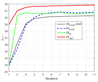
Figure 1: The $\sigma_{psnr}$ of the four different cases versus the iteration number on testing data.

Table 1: The CPU Time Of The Four Different Cases. (Seconds)

$CS_{S-DCS}-small$	$CS_{S-DCS}$	$CS_{BL}$	$CS_{Alg3}$
$2.79\times 10^{1}$	$1.32\times 10^{3}$	$4.33\times 10^{4}$	$1.54\times 10^{2}$

Benefiting from the large training dataset, $CS_{S-DCS}$ yields a better performance in terms of $\sigma_{psnr}$ than $CS_{S-DCS}-small$. This indicates that enlarging the training dataset leads to a better CS system. Compared with $CS_{S-DCS}-small$, $CS_{BL}$ has a higher $\varrho_{psnr}$ which meets the observation shown in [15]. However, $CS_{BL}$ needs many SVDs in the algorithm which makes it inefficient and hard to extend to the situation when the training dataset is large. This concern can be observed from Table 1 that $CS_{BL}$ needs much more CPU time even for only $6000$ training patches. Although $CS_{BL}$ has a better performance than $CS_{S-DCS}-small$, this advantage will disappear if we enlarge the size of the training dataset in $CS_{S-DCS}$. It can be seen from Fig. 1 that $CS_{S-DCS}$ has a similar performance with $CS_{BL}$, but it requires a shorter training time, see Table 1. $CS_{Alg3}$ has a best performance in terms of $\varrho_{psnr}$ compared with other methods. Meantime, $CS_{Alg3}$ has a relatively shorter CPU time but has the largest training dataset. It indicates that Algorithm 1 is suitable for training the SMSD on a large training dataset. Moreover, we observe that training on a large dataset can obtain a better SMSD and the proposed Algorithm 1 belongs to a good choice which takes the efficiency and effectiveness into account simultaneously.

Additionally, we also investigate the performance of the four different CS systems mentioned in this paper on ten natural images. The Structural Similarity Index (SSIM) [28] is also involved in comparing the recovered natural images by the different methods. As the results shown in Table 4, we see the proposed Algorithm $3$ yields the highest PSNR and SSIM. Compared with $CS_{S-DCS}-small$, $CS_{S-DCS}$ has a higher PSNR and SSIM on all of the ten testing natural images. This meets the argument in this paper that enlarging the size of the training dataset is significant in practice. This can also be illustrated by the methods between $CS_{BL}$ and $CS_{S-DCS}$. Note that $CS_{BL}$ works better than $CS_{S-DCS}-small$ when they have the same small size of training dataset. However, the performance of $CS_{S-DCS}$ will exceed $CS_{BL}$ when the size of the training data is enlarged. All of these imply that training the sensing matrix and the corresponding sparsifying dictionary on a large dataset is preferred. Moreover, the proposed Algorithm $3$ is a good choice to stand such a mission. To examine the visual effect clearly, the recovered performance of two natural images, i.e., ‘Lena’ and ‘Mandril’ in Fig. 2, are shown in Fig.s 3 and 4.

Table 2: Performance Evaluated With Four Cases Shown In This Paper. (Left: PSNR, Right: SSIM. The highest is marked with bold.)

	$CS_{S-DCS}-small$		$CS_{S-DCS}$		$CS_{BL}$		$CS_{Alg3}$
Lena	$33.0566$	$0.9089$	$33.7859$	$0.9184$	$33.3059$	$0.9111$	$\bm{34.6557}$	$\bm{0.9281}$
Elaine	$32.3990$	$0.8073$	$32.6903$	$0.8145$	$32.4076$	$0.8043$	$\bm{33.1756}$	$\bm{0.8244}$
Man	$31.1978$	$0.8738$	$31.8509$	$0.8866$	$31.4686$	$0.8782$	$\bm{32.5941}$	$\bm{0.8999}$
Mandrill	$23.4291$	$0.7598$	$23.8411$	$0.7823$	$23.8221$	$0.7746$	$\bm{24.3753}$	$\bm{0.8007}$
Peppers	$28.9462$	$0.8877$	$29.6975$	$0.9005$	$29.4145$	$0.8925$	$\bm{30.6859}$	$\bm{0.9169}$
Boat	$29.7350$	$0.8561$	$30.3488$	$0.8679$	$30.1027$	$0.8580$	$\bm{31.2858}$	$\bm{0.8837}$
House	$31.5166$	$0.8842$	$32.0602$	$0.8985$	$32.0707$	$0.8956$	$33.0146$	$\bm{0.9158}$
Cameraman	$26.2240$	$0.8581$	$26.8272$	$0.8716$	$26.4545$	$0.8673$	$\bm{27.4254}$	$\bm{0.8877}$
Barbara	$25.6148$	$0.8239$	$25.9153$	$0.8316$	$25.5165$	$0.8168$	$\bm{26.0835}$	$\bm{0.8393}$
Tank	$30.7233$	$0.8252$	$30.8210$	$0.8369$	$31.1403$	$0.8361$	$\bm{31.7818}$	$\bm{0.8576}$
Averaged	$29.2842$	$0.8485$	$29.7838$	$0.8609$	$29.5703$	$0.8534$	$\bm{30.5078}$	$\bm{0.8754}$

(a) ‘Lena’

(b) ‘Mandrill’

Figure 2: The original testing images.

(a) $CS_{S-DCS}-small$

(b) $CS_{S-DCS}$

(c) $CS_{BL}$

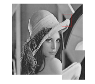
(d) $CS_{Alg3}$

Figure 3: The recovered testing image ‘Lena’.

(a) $CS_{S-DCS}-small$

(b) $CS_{S-DCS}$

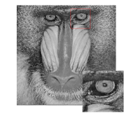
(c) $CS_{BL}$

(d) $CS_{Alg3}$

Figure 4: The recovered testing image ‘Mandrill’.

Now, we come to experimentally check the convergence of our proposed algorithm. In this experiment, we run another sufficient large iterations on dictionary updating after running Algorithm 1 to see whether the dictionary can converge. The testing error versus iteration on testing data is shown in Fig. 4. Clearly, even if the testing error is not monotonically decreasing, it is asymptotically decreasing which meets the property of our online algorithm (Proposition 1) because we randomly sample part of the training data to update the dictionary at each iteration. We can also observe that the recovery accuracy in terms of $\varrho_{psnr}$ on testing data is also increasing along the number of iterations growing. As seen from the sub-figure in Fig. 4, the recovered PSNR increases dramatically after the $1000$-th iteration, in which we update the sensing matrix again. Moreover, we see that the PSNR still increases as the iteration goes, which demonstrates the significance of our algorithm to simultaneously optimize the sensing matrix and the dictionary. We also display the difference of the dictionary between each iteration in Fig. 6. As observed from Fig. 6(a), there exist many oscillations which are caused by the fact that we update the dictionary through the stochastic method which only utilizes a part of training data in each iteration. If we check Fig. 6(b), the envelop of Fig. 6(a), we see it is convergent and coincides with the Proposition 2 that the stationary point can be attained. Note that all of the observations meet our previous statements in Section 3 regarding the convergence analysis of the proposed Algorithm 1. However, the whole investigation of the convergence analysis for Algorithm 1 is out of the scope in this paper and belongs to future work.

Figure 5: Objective value $\sigma(\bm{\Psi}_{t},\bm{\Theta}_{t})$ and $\sigma_{psnr}$ versus iteration on testing data through Algorithm $3$.

(a) The difference between each dictionary versus iteration .

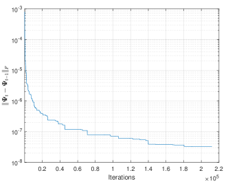
(b) The envelop of the difference between each dictionary versus iteration.

Figure 6: The change of each dictionary in each iteration.

5 Conclusion

In this paper, an efficient algorithm for jointly learning the SMSD on a large dataset is proposed. The proposed algorithm optimizes the sensing matrix with a closed-form solution and learns a sparsifying dictionary with a stochastic method on a large training dataset. Our experiment results show that training the SMSD on a large dataset yildes a better performance and the proposed method which considers the efficiency and effectiveness simultaneously is a suitable choice for such a task.

One of the possible directions for future research is to develop an accelerated algorithm to make the proposed method more efficient. Involving the Sequential Subspace Optimization (SESOP) in the algorithm may belong to one of the possible methods to realize the accelerated purpose [29].

Acknowledgment

This research is supported in part by ERC Grant agreement no. 320649, and in part by the Intel Collaborative Research Institute for Computational Intelligence (ICRI-CI). The code in this paper to represent the experiments can be downloaded through the link https://github.com/happyhongt/.

References

- [1] S. Mallat, A wavelet tour of signal processing: the sparse way, Academic press, 2008.
- [2] M. Elad, Sparse and Redundant Representations: from theory to applications in signal and image processing, Springer Science & Business Media, 2010.
- [3] I. Tosic and P. Frossard, “Dictionary Learning,” IEEE Signal Process. Mag., vol. 28, pp. 27-38, Mar. 2011.
- [4] K. Engan, S. O. Aase, and J. H. Hakon-housoy, “Method of optimal direction for frame design,” Proc. IEEE Int. Conf. Acoust., Speech, Signal Process., vol. 5, pp. 2443-2446, Mar. 1999.
- [5] M. Aharon, M. Elad, and A. Bruckstein, “K-SVD: An algorithm for designing overcomplete dictionaries for sparse representation,” IEEE Trans. Signal Process., vol. 54, pp. 4311-4322, Nov. 2006.
- [6] E. J. Candès and M. B. Wakin, “An introduction to compressive samping,” IEEE Signal Process. Mag., vol. 25, pp. 21-30, Mar. 2008.
- [7] Z. Zhu and M. B. Wakin, “Approximating sampled sinusoids and multiband signals using multiband modulated DPSS dictionaries,” J. Fourier Anal. Appl. pp. 1-48, 2016.
- [8] M. Elad, “Optimized projections for compressed sensing,” IEEE Trans. Signal Process., vol. 55, pp. 5695-5702, Dec. 2007.
- [9] G. Li, Z. H. Zhu, D. H. Yang, L. P. Chang, and H. Bai, “On projection matrix optimization for compressive sensing systems,” IEEE Trans. Signal Process., vol. 61, pp. 2887-2898, Jun. 2013.
- [10] G. Li, X. Li, S. Li, H. Bai, Q. Jiang and X. He, “Designing robust sensing matrix for image compression,” IEEE Trans. Image Process., vol. 24, pp. 5389-5400, Dec. 2015.
- [11] T. Hong, H. Bai, S. Li and Z. Zhu, “An efficient algorithm for designing projection matrix in compressive sensing based on alternating optimization,” Signal Process., vol. 125, pp. 9-20, Aug. 2016.
- [12] W. Chen, M. R. D. Rodrigues and I. J. Wassell, “Projection Design for Statistical Compressive Sensing: A Tight Frame Based Approach,” IEEE Trans. Signal Process., vol. 61, no. 8, pp. 2016-2029, Apr. 2013.
- [13] T. Hong and Z. Zhu, “An Efficient Method for Robust Projection Matrix Design,” Signal Process., vol. 143, pp. 200-210, Feb. 2018.
- [14] J. M. Durate-Carvajalino and G. Sapiro, “Learning to sense sparse signals: simultaneously sensing matrix and sparsifying dictionary optimization,” IEEE Trans. Image Process., vol. 18, pp. 1395-1408, Jul. 2009.
- [15] H. Bai, G. Li, S. Li, Q. Li, Q. Jiang, and L. Chang, “Alternating optimization of sensing matrix and sparsifying dictionary for compressed sensing,” IEEE Trans. Signal Process., vol. 63, pp. 1581-1594, Mar. 2015.
- [16] G. Li, Z. Zhu, X. Wu, and B. Hou, “On joint optimization of sensing matrix and sparsifying dictionary for robust compressed sensing systems,” Digital Signal Process., vol. 73, pp. 62–71, 2018.
- [17] Z. Zhu, G. Li, J. Ding, Q. Li, and X. He, “On Collaborative Compressive Sensing Systems: The Framework, Design and Algorithm,” to appear in SIAM Journal on Imaging Sciences, 2018.
- [18] J. Mairal, F. Bach, J. Ponce, and G. Sapiro, “Online dictionary learning for sparse coding,” Proceedings of the 26th international conference on machine learning, ACM, pp. 689-696, Jun. 2009.
- [19] J. Mairal, F. Bach, J. Ponce, and G. Sapiro, “Online learning for matrix factorization and sparse coding,” Journal of Machine Learning, vol. 11, pp. 19-60, Jan. 2010.
- [20] Wu-Sheng Lu, and H. Takao. ”Design of projection matrix for compressive sensing by nonsmooth optimization.” Circuits and Systems (ISCAS), 2014 IEEE International Symposium on. IEEE, 2014.
- [21] M. Sadeghi and B.Z. Massoud, “Incoherent unit-norm frame design via an alternating minimization penalty method,” IEEE Signal Process. Letters, vol. 24, pp. 32-36, Jan. 2017.
- [22] R. A. Horn and C. R. Johnson, Matrix Analysis, Cambridge University, Second Edition, 2012.
- [23] Z. Zhu, Q. Li, G. Tang, and M. B. Wakin, “Global Optimality in Low-rank Matrix Optimization,” EEE Transactions on Signal Process., vol. 66 (13), pp. 3614-3628, 2018.
- [24] L. Bottou, “Large-scale machine learning with stochastic gradient descent,” Proceedings of COMPSTAT’2010. Physica-Verlag HD, pp. 177-186, 2010.
- [25] J. Sulam, B. Ophir, M. Zibulevsky and M. Elad, “Trainlets: Dictionary learning in high dimensions,” IEEE Transactions on Signal Process., vol. 64, pp. 3180-3193, Mar. 2016.
- [26] J. Sulam and M. Elad, “Large inpainting of face images with trainlets,” IEEE Signal Process. Letters, vol. 23, pp. 1839-1843, Oct. 2016.
- [27] B. C. Russell, A. Torralba, K. P. Murphy, and W. T. Freeman, “LabelMe: A Database and Web-Based Tool for Image Annotation,” International Journal of Computation Vision, vol. 77, pp. 157-173, May 2008.
- [28] Z. Wang, A. C. Bovik, H. R. Sheikh, and E. P. Simoncelli, “Image quality assessment: from error visibility to structural similarity,” IEEE Trans. Image Process., vol. 13, pp. 600-612, Apr. 2004.
- [29] E. Richardson, R. Herskovitz, B. Ginsburg, and M. Zibulevsky, “SEBOOST-Boosting stochastic learning using subspace optimization techniques,” Advanced in Neural Information Process. Systems, NIPS, 2016.