Second-order numerical methods for multi-term fractional differential equations: Smooth and non-smooth solutions

Abstract

Starting with the asymptotic expansion of the error equation of the shifted Grünwald–Letnikov formula, we derive a new modified weighted shifted Grünwald–Letnikov (WSGL) formula by introducing appropriate correction terms. We then apply one special case of the modified WSGL formula to solve multi-term fractional ordinary and partial differential equations, and we prove the linear stability and second-order convergence for both smooth and non-smooth solutions. We show theoretically and numerically that numerical solutions up to certain accuracy can be obtained with only a few correction terms. Moreover, the correction terms can be tuned according to the fractional derivative orders without explicitly knowing the analytical solutions. Numerical simulations verify the theoretical results and demonstrate that the new formula leads to better performance compared to other known numerical approximations with similar resolution.

1 Introduction

The aim of this work is to provide an effective numerical method to solve multi-term fractional differential equations (FDEs), where more than one fractional differential operator is involved, with high-order accuracy for both smooth and non-smooth solutions.

Multi-term FDEs are motivated by their flexibility to describe complex multi-rate physical processes, see e.g. [9, 18, 28, 34]. Moreover, it is not straightforward to extend the known numerical methods for single-term FDEs to solve multi-term FDEs. Specifically, we find that: (i) Some numerical methods for single-term FDEs can be extended to multi-term FDEs, but their numerical stability and convergence analysis are not easy to prove; (ii) Very low accurate numerical solutions may be obtained by extending the majority of the known numerical methods for single-term FDEs to multi-term FDEs due to their often unreasonable requirement on the high regularity of the solutions.

Existing numerical methods for FDEs can be broadly divided into two classes.

• FDEs with smooth solutions: The majority of numerical methods have been developed for single-term FDEs with smooth solutions, in which the fractional derivative operators in these equations are discretized by the (shifted) Grünwald–Letnikov (GL) formula [5, 17, 31, 34], the L1 method and its modification [24, 50], the weighted shifted Grünwald–Letnikov (WSGL) formulas [39, 41], the (weighted) fractional central difference methods [4, 12, 13, 52], the fractional linear multi-step methods [8, 26, 43, 45, 46, 47, 49], the spectral approximations [44, 48, 53], and so on [6, 16, 32, 38]. Some of these methods have been extended to solve multi-term FDEs with smooth solutions, such as the L1 method in time with spatial discretization by the finite difference method (see e.g. [25, 37]) and finite element method (see e.g. [20]), the predictor-corrector method in time with finite difference methods in space [25, 42], and some others [15, 33], just to name a few.

• FDEs with non-smooth solutions: Generally speaking, the analytical solutions to FDEs are not smooth in real applications. For example, even for smooth inputs, the solutions to FDEs usually have a weak singularity at the boundary, see e.g. [9, 21, 28, 29, 40, 51]. Therefore, the aforementioned numerical methods will produce numerical solutions of low accuracy when applied to solve these FDEs. In order to derive numerical schemes of uniformly high-order convergence for FDEs with non-smooth solutions, several approaches have been proposed:

  • Use nonuniform/refined grids in the discretization of the fractional operators, see e.g. [30, 32, 36, 50]). With a geometrically graded mesh, one can adaptively resolve a weak singularity at the endpoint.

  • Separate the solution $U$ of the considered FDE into two parts of $U^{(1)}$ and $U^{(2)}$, satisfying $U=U^{(1)}+U^{(2)}$ (see e.g. [26, 45, 47]). Then, a numerical scheme is designed such that high accuracy is obtained for both $U=U^{(1)}$ and $U=U^{(2)}$.

  • Use a non-polynomial (or singular) basis function to capture the singularity of the solutions to FDEs (see e.g. [3, 7, 14, 16, 21, 29, 44, 48, 51]), such that a high-order scheme is effective.

We also note that many numerical methods for FDEs may impose some unreasonable restrictions on the solutions. For example, the L1 method (see e.g. [24]) and the interpolation method (e.g. [9, 38]) require that the solution of the considered FDE is sufficiently smooth such that the expected accuracy can be realized, but as we already stated solutions of FDEs are usually not smooth, see e.g. [9]. The second-order WSGL formula (see, e.g. [39, 41]) requires that the solution and its first (and/or second) derivative have vanishing values at the boundary; see also the corresponding works in [4, 6, 12, 13, 17, 46, 52, 54]. Consequently, the convergence rate of these methods can be low even if the solutions are sufficiently smooth. In particular, we show numerically that the second-order WSGL formula in [39, 41] does not exhibit global second-order accuracy for smooth solutions; see numerical results in Table 11. The theoretical explanation can be found in Section 2.

To remove these restrictions, we will adopt the approach (b2) to solve multi-term FODEs and multi-term time-fractional anomalous diffusion equations with smooth and non-smooth solutions. We note that the analytical solutions of FODEs and time-fractional differential equations usually have the form

$$U(t)=U^{(1)}(t)+U^{(2)}(t),\,U^{(1)}(t)=\sum_{r=0}^{m}c_{m}t^{\sigma_{r}},\,U^{(2)}(t)=c_{m+1}t^{\sigma_{m+1}}+u(t)t^{\sigma_{m+2}},\quad$$ (1)

where $u(t)$ is a uniformly continuous function over the interval $[0,T]$, $T>0$ and $0\leq\sigma_{r}<\sigma_{r+1},\,r=1,2,...,m$ and $m$ is a positive integer, see e.g. [8, 9, 11, 18, 19, 23, 28, 30]. Moreover, $\sigma_{1}$, $\ldots$, $\sigma_{m}$ are explicitly known, see e.g. [9, 11]. The WSGL formula in [39, 41] is indeed of second-order convergence for $U^{(2)}(t)$ when $\sigma_{m+1}\geq 2+\alpha$ ($\alpha$ is the fractional order) while it converges slowly for $U^{(1)}(t)$. This observation motivated us to apply the the idea of [26] in (b2) to obtain desired high accuracy schemes. Specifically, we introduce some corrections terms into the WSGL formula so that the resulting modified WSGL formula is exact or highly accurate for $U^{(1)}(t)$ while the second-order convergence for $U^{(2)}(t)$ is maintained.

According to [26], the correction terms are found using the so-called starting weights and values to make the resulting formula exact for low regularity terms $t^{\sigma_{r}}(1\leq r\leq m)$ in $U$ (see (1)). We need to solve a linear system to obtain the starting weights, whose coefficient matrix is an ill-conditioned exponential Vandermonde matrix. It has been pointed out in [10] that the accuracy in solving the corresponding weights “may have serious adverse effects for the entire scheme” when $m$ is large. However, it is shown in [10, 26] that the accuracy of Lubich’s correction approach depends on the residual of the linear system for obtaining the starting weights, which was discussed in detail in [10].

Fortunately, the number of correction terms can be small and still obtain reasonable accuracy. In this paper, we show that several correction terms (less than ten) significantly improve accuracy, regardless of the regularity of the analytical solution. Since we are using a few corrections terms, the condition number of the exponential Vandermonde matrices is not too large and thus the linear system to derive the starting weights can be solved accurately with double precision. Moreover, even if the regularity indices $\sigma_{r}$ (see (1)) are unknown and the “correction terms” do not match the singularity of the analytical solutions to considered FDEs, we can still obtain satisfactory accuracy, see Example 2.1 and numerical results in Section 5. In particular, we present in Lemma 2 a detailed error estimate of the WSGL formula with correction terms, which explains why a few correction terms may lead to satisfactory accuracy.

We organize the paper as follows. In Section 2, we obtain the asymptotic error equation of the shifted GL formula that leads to the second-order WSGL formula under mild conditions. We then show that the WSGL formula with correction terms can lead to better accuracy. In Section 3, we apply one special case of the second-order WSGL formula with correction terms to multi-term FODEs and present the stability and convergence theory. We further extend the second-order WSGL formula with correction terms in Section 4 to the time discretization of the multi-term time-fractional diffusion-wave equation together with the spectral element method for spatial discretization. Numerical results for smooth and non-smooth solutions are included in Section 5. All the proofs of our lemmas and theorems are presented in Section 6 before the conclusion in the last section. In the Appendix we include some computational details, additional proofs, and also more numerical results.

2 Finite difference approximations for fractional derivatives

In this section, we examine the asymptotic behavior of the error equation of the shifted GL formula, which leads to the error estimate of the WSGL formula [39]. Following Lubich’s approach [26], we then introduce correction terms to recover the global second-order accuracy of the WSGL formula and obtain an error bound.

We first introduce definitions of fractional integrals and derivatives. The $\alpha$th-order Caputo derivative operator is defined [34]

$${}_{C}D^{\alpha}_{0,t}{U(t)}=D^{-(n-\alpha)}_{0,t}\left[D^{n}U(t)\right]=\frac{1}{\Gamma(n-\alpha)}\int_{0}^{t}(t-s)^{n-\alpha-1}\frac{\,{\rm d}^{n}}{\,{\rm d}s^{n}}U(s)\,{\rm d}s,$$ (2)

where $n-1<\alpha\leq n$, $n$ is a positive integer. The fractional integral $D^{-\gamma}_{0,t}$ is given by

$$D^{-\gamma}_{0,t}U(t)={}_{RL}D^{-\gamma}_{0,t}U(t)=\frac{1}{\Gamma(\gamma)}\int_{0}^{t}(t-s)^{\gamma-1}{U(s)}\,{\rm d}s,{\quad}\gamma>0.$$ (3)

Let $\tau>0$ be a time stepsize and $n_{T}$ be a positive integer with $\tau=T/n_{T}$ and $t_{n}=n\tau(n=0,1,...,n_{T}$). The shifted GL formula (with $q$ shifts) reads (see e.g. [31]):

$$\mathcal{B}^{\alpha,n}_{q}U=\frac{1}{\tau^{\alpha}}\sum_{k=0}^{n+q}\omega^{(\alpha)}_{k}U(t_{n-k+q})=\frac{1}{\tau^{\alpha}}\sum_{k=0}^{n+q}\omega^{(\alpha)}_{k}U^{n-k+q},$$ (4)

where $\omega^{(\alpha)}_{k}=(-1)^{k}\binom{\alpha}{k}$. We have the following error estimate for the formula (4), the proof of which can be found in Section 6.

Lemma 1 (Error of the shifted GL formula (4)).

Let $U(t)=t^{\sigma}\,(\sigma\geq 0)$ and $\alpha$ be a real number. Then

$$\left[{}_{RL}D^{\alpha}_{0,t}U(t)\right]_{t=t_{n}}=\mathcal{B}^{\alpha,n}_{q}U-\tau\left(q-\frac{\alpha}{2}\right)\frac{\Gamma(\sigma+1)}{\Gamma(\sigma-\alpha)}t_{n}^{\sigma-1-\alpha}+\tau^{2}R^{n,\alpha,\sigma},$$ (5)

where $\mathcal{B}^{\alpha,n}_{q}$ is defined by (4), $n\geq|q|$, $q$ is an integer, and $R^{n,\alpha,\sigma}$ is bounded by

$$\left|R^{n,\alpha,\sigma}\right|\leq Ct_{n}^{\sigma-2-\alpha}.$$ (6)

Here and throughout the paper, the constant $C>0$ is independent of $n$ and $\tau$.

From Lemma 1, we can eliminate the term $t_{n}^{\sigma-1-\alpha}$ in (5) by a linear combination of $\mathcal{B}_{q}^{\alpha,n}$ and $\mathcal{B}_{p}^{\alpha,n}$, $p\neq q$. Let

$$\mathcal{A}_{p,q}^{\alpha,n}U=\frac{\alpha-2q}{2(p-q)}\mathcal{B}^{\alpha,n}_{p}U+\frac{2p-\alpha}{2(p-q)}\mathcal{B}^{\alpha,n}_{q}U.$$ (7)

Then we obtain the second-order WSGL formula in [39],

$$\left[{}_{RL}D_{0,t}^{\alpha}U(t)\right]_{t=t_{n}}=\mathcal{A}_{p,q}^{\alpha,n}U+\tau^{2}R^{n,\alpha,\sigma},\quad|R^{n,\alpha,\sigma}|\leq Ct_{n}^{\sigma-2-\alpha}.$$ (8)

Eq. (7) is proved in [39, 41] to be of second-order convergence when $U(0)=0$, ${}_{RL}D_{0,t}^{\alpha+2}U(t)$ and its Fourier transform belongs to $L_{1}(\mathbb{R})$. However, these conditions are too restrictive since ${}_{RL}D_{0,t}^{\alpha+2}U(t)\notin L_{1}(\mathbb{R})$ for $U(t)=t^{\sigma_{r}}$ with $0\leq\sigma_{r}\leq 1+\alpha$ when $\alpha>0$. For example, when $U(t)=t$, the remainder term in (8) is of the order of $\tau^{2}t_{n}^{-1-\alpha}$, which is not of second-order convergence globally as the accuracy is $O(\tau^{1-\alpha})$ when $t_{n}=\tau$. Consequently, when (8) is applied to solve FDEs with even smooth solutions, we cannot expect a global second-order convergence unless the solutions have vanishing first-order derivatives. In particular, there is almost no accuracy at $t=0$ when $1<\alpha<2$. In practice, this large error near $t=0$ may lead to large accumulation of discretization errors and thus much larger error at the desired final time $t_{n}$; see accuracy tests of the formula (7) in Fig. 1 of this section and numerical experiments in Section 5.

To improve the accuracy near $t=0$, we follow Lubich’s approach [26] by adding correction terms to (7) such that the resulting formula is indeed of second-order accuracy when $U(t)$ is of the form (1). Specifically, we modify (7) such that

$$\left[{}_{RL}D_{0,t}^{\alpha}U(t)\right]_{t=t_{n}}=\mathcal{{A}}_{p,q}^{\alpha,n,m}U+R^{n},\,\,\,\mathcal{{A}}_{p,q}^{\alpha,n,m}U=:\mathcal{A}_{p,q}^{\alpha,n}U+\frac{1}{\tau^{\alpha}}\sum_{k=1}^{m}w_{n,k}^{(\alpha)}U(t_{k}).$$ (9)

In (9), the starting weights $\{w_{n,k}^{(\alpha)}\}$ are known at each time step as they can be determined by setting $R^{n}=0$ in (9) for $U(t)=t^{\sigma_{r}}\,(1\leq r\leq m)$. Denote $\displaystyle\mathcal{A}_{p,q}^{\alpha,n}U=\frac{1}{\tau^{\alpha}}\sum_{k=0}^{n}g^{(\alpha)}_{n-k}U(t_{k})$. Then the starting weights can be solved from the following linear system of equations, see e.g. [10, 26],

$$\sum_{k=1}^{m}w_{n,k}^{(\alpha)}k^{\sigma_{r}}=\frac{\Gamma(\sigma_{r}+1)}{\Gamma(\sigma_{r}+1-\alpha)}n^{\sigma_{r}-\alpha}-\sum_{k=0}^{n}g^{(\alpha)}_{n-k}k^{\sigma_{r}},\quad 1\leq r\leq m.$$ (10)

The linear system (10) has an exponential Vandermonde type matrix that is ill-conditioned when $m$ is large [10]. The large condition number of the matrix may lead to big roundoff errors of $w_{n,r}^{(\alpha)}$ $(1\leq r\leq m)$ when computation is performed with double precision. For $\sigma_{k}=k\alpha$, we present the condition number of the system (10) in Table 1. Hereafter we choose $(p,q)=(0,-1)$ in (9) where the quadrature weights $g^{(\alpha)}_{k}$’s are defined by, see [26, 39, 41],

$$g^{(\alpha)}_{0}=\frac{2+\alpha}{2}\omega^{(\alpha)}_{0},{\quad}g^{(\alpha)}_{k}=\frac{2+\alpha}{2}\omega^{(\alpha)}_{k}-\frac{\alpha}{2}\omega^{(\alpha)}_{k-1},\quad\omega^{(\alpha)}_{k}=(-1)^{k}\binom{\alpha}{k},\,k\geq 1.$$ (11)

In fact, $g^{(\alpha)}_{k}$ satisfies $(1-z)^{\alpha}\left(1+\frac{\alpha}{2}-\frac{\alpha}{2}z\right)=\sum_{k=0}^{\infty}g^{(\alpha)}_{k}z^{k}$, see [26].

From Table 1, we observe that the condition number increases with $m$ and decreases with $\alpha$. However, for $m$ and $\alpha$’s presented in Table 1, we can still have some reasonable accuracy for the starting weights. In fact, the accuracy of (9) is determined somehow by the residual of (10). This observation has been made in [10, 26]. We present the residual of the system (10) in Table 2, where the residual is computed by $\max_{1\leq r\leq m,\,1\leq n\leq 100}|\sum_{k=1}^{m}w_{n,k}^{(\alpha)}k^{\sigma_{r}}-\frac{\Gamma(\sigma_{r}+1)}{\Gamma(\sigma_{r}+1-\alpha)}n^{\sigma_{r}-\alpha}+\sum_{k=0}^{n}g^{(\alpha)}_{n-k}k^{\sigma_{r}}|.$ When $\alpha=0.05$ and $m=7$, the condition number is $1.84\times 10^{12}$ and the residual is $1.19\times 10^{-6}$, see Table 2. In this case we can still obtain relatively high accuracy, see Figure 2.1(a) in Example 2.1.

Table 1: Condition numbers of the linear system (10), $\sigma_{k}=k\alpha\,(k\geq 1)$, and $(p,q)=(0,-1)$ in (9).

$\alpha$	$m=2$	$m=3$	$m=4$	$m=5$	$m=6$	$m=7$	$m=8$
$0.05$	1.15e+02	1.28e+04	1.41e+06	1.54e+08	1.69e+10	1.84e+12	2.02e+14
$0.1$	5.80e+01	3.20e+03	1.76e+05	9.72e+06	5.41e+08	3.04e+10	1.73e+12
$0.3$	2.03e+01	3.87e+02	7.86e+03	1.73e+05	4.12e+06	1.04e+08	2.81e+09

Table 2: The residual of the linear system (10), $\sigma_{k}=k\alpha\,(k\geq 1)$.

$\alpha$	$m=2$	$m=3$	$m=4$	$m=5$	$m=6$	$m=7$	$m=8$
$0.05$	1.66e-15	2.27e-13	7.27e-12	4.65e-10	2.60e-08	1.19e-06	6.86e-05
$0.1$	1.77e-15	2.84e-14	4.54e-13	5.82e-11	4.65e-10	1.11e-08	8.34e-07
$0.3$	1.11e-16	7.10e-15	5.68e-14	2.27e-13	1.81e-11	4.65e-10	6.05e-09

In our numerical simulations of this work, we choose less than eight correction terms. It works surprisingly well with high accuracy even when $\alpha$ is small. For example, in Figure 2.1(a), we used six correction terms for $\alpha=0.05$, the accuracy for all $t\geq 0.2$ is at the level of $10^{-8}$, which is two orders of magnitude lower than $\tau^{2}=10^{-6}$. Hence, we are motivated to consider the asymptotic behavior of $R^{n}$ in (9) when $U(t)=t^{\sigma}$, addressing the practical effect of correction terms.

Lemma 2.

Let $U(t)=t^{\sigma}\,(\sigma\geq 0)$ and $\alpha$ be a real number. Let $R^{n}$ be defined in $\eqref{s31-1-3}$, $S_{m}^{\sigma}=\prod_{k=1}^{m}|\sigma-\sigma_{k}|$, $\sigma_{\max}=\max\{\sigma,\sigma_{1},...,\sigma_{m}\}$. Then we have

$${\left|R^{n}\right|}\leq{\tau^{\sigma-\alpha}}\left[CS_{m}^{\sigma}\left(n^{\sigma-\alpha-2}\log^{m}(n)+n^{\sigma_{\max}-\alpha-2}\right)+\widetilde{C}{n}^{\sigma_{\max}-2-d-\alpha}\right],$$ (12)

where $C$ and $\widetilde{C}$ are positive constants bounded and independent of $n$ and $\tau$.

Remark 1.

Numerical results indicate that $R^{n}$ in (12) can be bounded by ${|R^{n}|}\leq CS_{m}^{\sigma}{\tau^{\sigma-\alpha}}n^{\sigma_{\max}-\alpha-2}.$ See the supplementary material.

From Lemmas 2 and 8, we have a uniformly second-order approximation $\mathcal{{A}}_{0,-1}^{\alpha,n,m}U$ of $\left[{}_{RL}D_{0,t}^{\alpha}U(t)\right]_{t=t_{n}}$ when $U(t)$ satisfies (1) and $\sigma_{m+1}\geq 2+\alpha$, i.e., $|R^{n}|\leq C\tau^{2}t_{n}^{\sigma_{m+1}-2-\alpha}$. In practice, especially with double precision computation, we take only small $m$ and thus $\sigma_{m+1}\geq 2+\alpha$ may not hold. In this case, we may not have the global second-order accuracy, but we still observe accuracy improvement at $t=0$ and small errors far from $t=0$ due to the small coefficient $S_{m}^{\sigma}$ in (12).

Next, we check the accuracy of the discrete operator $\mathcal{{A}}_{0,-1}^{\alpha,n,m}$ in (9).

Example 2.1.

Use the formula (9) with $(p,q)=(0,-1)$ to numerically approximate ${}_{RL}D_{0,t}^{\alpha}U(t)$. We consider two cases: Case I: $U(t)=t^{8\alpha}$, where we take $\sigma_{k}=k\alpha$, $k\leq 8$. Case II: $U(t)=t^{8\alpha}+t^{9\alpha}+t^{10\alpha}+t^{11\alpha}$, where we take $\sigma_{k}=(k+7)\alpha$.

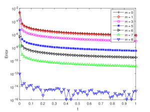
(a) $\alpha=0.05$.

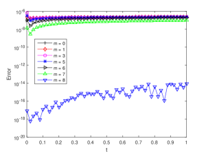
(b) $\alpha=0.3$.

Fig. 1: Pointwise errors of $\mathcal{A}_{0,-1}^{\alpha,n,m}$ for Example 2.1, Case I, $\tau=10^{-3}$; small value of fractional order (left) and larger value (right).

Table 3: Values of $S^{\sigma}_{m}$ for Case I, $\sigma=8\alpha$, and $\sigma_{k}=k\alpha\,(k\geq 1)$.

$\alpha$	$m=1$	$m=3$	$m=5$	$m=6$	$m=7$	$m=8$
$0.05$	3.50e-1	2.62e-2	7.88e-4	7.88e-5	3.94e-6	0
$0.1$	7.00e-1	2.10e-1	2.52e-2	5.04e-3	5.04e-4	0
$0.3$	2.10e-0	5.67e-0	6.12e-0	3.67e-0	1.10e-0	0

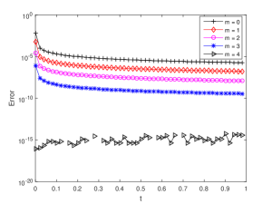
(a) $\alpha=0.05$.

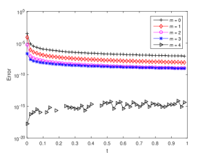
(b) $\alpha=0.1$.

Fig. 2: Pointwise errors of $\mathcal{A}_{0,-1}^{\alpha,n,m}$ for Example 2.1, Case II, $\tau=10^{-3}$.

The purpose of this example is to show that a small number of correction terms is sufficient to yield relatively high accuracy whether $U(t)$ has high regularity or not.

We first consider Case I. When $\alpha$ is small, the regularity of $U(t)$ is low. In such a case, we add only several correction terms but obtain satisfactory accuracy, see Fig. 1 (a). The accuracy can be explained by the estimate $S^{\sigma}_{m}\tau^{2}t_{n}^{\sigma-\alpha-2}$ in Lemma 2, especially the factor $S^{\sigma}_{m}$ in the error estimate. Despite the accuracy from $\tau^{2}t_{n}^{\sigma-\alpha-2}$, the factor $S_{m}^{\sigma}=7\times 6\times\cdots\times(8-m)\alpha^{m}$ is very small when $\alpha$ is small and $m$ is large, see Table 3. The small factor $S^{\sigma}_{m}$ explains the high accuracy in Figs. 1 (a). When $\alpha$ is relatively large, we need only several terms to achieve second-order accuracy according to (9) and Lemma 2. In this case, the term $\tau^{2}t_{n}^{\sigma-\alpha-2}$ is more pronounced than $S_{m}^{\sigma}$, see Table 3. This effect is shown in Fig. 1 (b), where we observe that increasing the number of correction terms does not increase accuracy significantly except for $m=8$, due to high regularity of $U(t)$.

For Case II, we choose $\sigma_{k}$ so that we match more terms of the singularity in $U(t)$; the pointwise errors are shown in Fig. 2. We obtain better accuracy as the number of correction terms $m$ increases up to $4$ when we capture all the singularity of $U(t)$ that leads to accuracy at the machine precision level.

In conclusion, we find that only a few number of corrections are needed to obtain high accuracy even when $U(t)$ has low regularity at $t=0$. We also find that we do not have to match the singular terms in $U(t)$ when choosing correction terms. In Section 5, we will present numerical examples with some empirical guidelines to introduce correction terms where we do not know explicitly the singular terms in $U(t)$.

3 Application to multi-term FODEs

In this section, we apply the formula (9) to the discretization of multi-term FODEs of the form

$$\sum_{j=1}^{Q}\nu_{j}{}_{C}D_{0,t}^{\alpha_{j}}Y(t)=f(t,Y),{\quad}t\in(0,T],T>0,{\quad}Y(0)=Y_{0},$$ (13)

where $\nu_{1}>0,\nu_{j}\geq 0\,(2\leq j\leq Q)$, and $0<\alpha_{j+1}\leq\alpha_{j}\leq 1\,(1\leq j<Q)$. The existence, uniqueness, and regularity of solutions to (13) are investigated in [9, 23, 28]. If $f(t,Y(t))$ is smooth for $t\in(0,T]$ or $f(t,Y(t))=-Y(t)$, $\{\alpha_{j}\}$ are rational numbers (see e.g. [9, 18, 19, 28]), then the solution $Y(t)$ to (13) has the form

$$Y(t)-Y(0)=c_{1}t^{\sigma_{1}}+c_{2}t^{\sigma_{2}}+c_{3}t^{\sigma_{3}}+\cdots,{\quad}\sigma_{k}<\sigma_{k+1},k>0.$$ (14)

Using ${}_{C}D_{0,t}^{\alpha_{j}}Y(t)={{}_{RL}D_{0,t}^{\alpha_{j}}}(Y(t)-Y(0))$, we apply (9) to (13) that leads to

$$\sum_{j=1}^{Q}{\nu_{j}}\mathcal{{A}}_{0,-1}^{\alpha_{j},n,m_{j}}\widehat{Y}=f(t_{n},Y(t_{n}))+R^{n},$$ (15)

where $\widehat{Y}(t)=Y(t)-Y(0)$, $\mathcal{{A}}_{0,-1}^{\alpha_{j},n,m_{j}}$ is defined by (9), and $m_{j}\,(1\leq j\leq Q)$ are suitable positive integers. By (9), the truncation error $R^{n}$ in (15) satisfies $R^{n}=\sum_{j=1}^{Q}O(\tau^{2}t_{n}^{\sigma_{m_{j}+1}-2-\alpha_{j}})$. Let $y^{n}$ be the approximate solution of $Y(t_{n})$. Then we derive the following fully discrete scheme for (13)

$$\sum_{j=1}^{Q}{\nu_{j}}\mathcal{{A}}_{0,-1}^{\alpha_{j},n,m_{j}}\hat{y}=f(t_{n},y^{n}),{\quad}y^{0}=Y_{0},$$ (16)

where $\hat{y}=y-y^{0}$ and $\mathcal{{A}}_{0,-1}^{\alpha_{j},n,m_{j}}$ is from (9). Denote $m=\max\{m_{1},m_{2},...,m_{Q}\}$.

Remark 2.

We need numerical values $y^{k}(k=1,2,...,m)$ to proceed with the scheme. Here we solve the nonlinear system of $y^{k}(k=1,2,...,m)$ using (16) with $n=1,2,...,m$, and we apply the Picard fixed-point iteration method. Other high-order methods for $y^{k}(k=1,2,...,m)$ can be applied here too.

Next, we present the stability and convergence for (16), the proofs of which are given in Section 6.

Theorem 3 (Linear stability).

If $f(t,Y)=-\lambda Y(t),Re(\lambda)>0$, then the method (16) is unconditionally stable.

Theorem 4 (Convergence).

Let $y^{n}$ be the solution to (16) and $Y(t)$ be the solution to (13) satisfying $Y(t)-Y(0)=c_{1}t^{\sigma_{1}}+c_{2}t^{\sigma_{2}}+...$, where $\{c_{k}\}$ are constants and $0<\sigma_{k}<\sigma_{k+1},k>0$. Suppose that $f(t,Y)$ satisfies the Lipschitz condition in its second argument, $m_{j}\,(j=1,2,...,Q)$ are suitable positive constants satisfying $\sigma_{m_{j}}\leq 2$. Then there exists a positive constant $C$ independent of $n$ and $\tau$ such that

$$|Y(t_{n})-y^{n}|\leq C\bigg{(}\sum_{k=0}^{\max\limits_{1\leq j\leq Q}\{m_{j}\}}|Y(t_{k})-y^{k}|+\tau^{\min\big{\{}2,\min\limits_{1\leq j\leq Q}\{\sigma_{m_{j}+1}+\alpha_{1}-\alpha_{j}\}\big{\}}}\bigg{)}.$$ (17)

Theorem 5 (Average error estimate).

Let $q=\min_{1\leq j\leq Q}\{\sigma_{m_{j}+1}-\alpha_{j}\}$. If $f(t,Y)=-Y(t)$ in Theorem 4, then we have for $K\geq 1$,

$$\bigg{(}\tau\sum_{n=1}^{K}|e^{n}|^{2}\bigg{)}^{\frac{1}{2}}\leq C\tau^{\min\{2,q+\frac{1}{2}\}}+C\max_{1\leq r\leq m}|e^{r}|\sum_{j=1}^{Q}\tau^{\frac{1}{2}-\alpha_{j}}K^{\max\{0,\sigma_{m}-\alpha_{j}-\frac{3}{2}\}}.$$ (18)

Two special cases of Theorem 5 are presented below. If there is no correction terms, i.e., $m_{j}=0$, then we have

$$\bigg{(}\tau\sum_{n=1}^{K}|e^{n}|^{2}\bigg{)}^{1/2} \leq C\tau^{\min\{2,q+0.5\}}=C\tau^{\min\{2,\sigma_{1}-\alpha_{1}+0.5\}}.$$ (19)

If $m_{j}=m$ and $\max_{1\leq r\leq m}|e^{r}|\leq C\tau^{\sigma_{m+1}}$, then we have

$$\bigg{(}\tau\sum_{n=1}^{K}|e^{n}|^{2}\bigg{)}^{1/2} \leq C\tau^{\min\{2,\sigma_{m+1}-\alpha_{1}+0.5\}}.$$ (20)

4 Application to time-fractional diffusion-wave equation

In this section, we consider the following time-fractional diffusion-wave equation, see e.g. [1, 25]:

$$\left\{\begin{aligned} &\partial_{t}^{2}U+\nu\,{}_{C}D_{0,t}^{1+\alpha}U=\mu\,\partial_{x}^{2}U+f(x,t),{\quad}(x,t){\,\in\,}\Omega{\times}(0,T],T>0,\\ &U(x,0)=\phi_{0}(x),{\quad}\partial_{t}U(x,0)=\psi_{0}(x),{\quad}x{\,\in\,}\bar{\Omega},\\ &{U(x,t)=0,{\quad}(x,t){\,\in\,}\partial\Omega\times(0,T]},\end{aligned}\right.$$ (21)

where $0<\alpha\leq 1,\,\nu\geq 0,\mu>0$, $\Omega=(a,b)$. We apply the quadrature formula (9) in time and spectral element method in space for the discretization of Eq. (21). We also present the rigorous stability and convergence analysis of the present numerical scheme, the proofs of which can be found in the supplementary material.

The key assumption here is that the analytical solution $U(t)=U(x,t)$ to (21) satisfies the following form

$$U(t)-U(0)-t\partial_{t}U(0)=\sum_{r=1}^{m}c_{r}(x)t^{\sigma_{r}}+c_{m+1}(x)t^{\sigma_{m+1}}+\cdots,$$ (22)

where $1<\sigma_{r}<\sigma_{r+1}$. Indeed, when $f(x,t)$ is smooth in time and $\alpha$ is rational, the analytical solution of (21) has the form as (22), see e.g. [9].

4.1 Time discretization

Denote $V(x,t)=\partial_{t}U(x,t)$, where $U(x,t)$ satisfies (22). Then $V(t)=V(x,t)$ satisfies $V(t)-V(0)=\sum_{r=1}^{m+1}d_{r}(x)t^{\sigma_{r}-1}+\cdots.$ Hence, we derive from (21)

$$\partial_{t}V(t)+\nu\,{}_{RL}D_{0,t}^{\alpha}(V(t)-V(0)) = \mu\,\partial_{x}^{2}U(t)+f(t),$$ (23)

$$\partial_{t}\partial_{x}^{2}U(t) = \partial_{x}^{2}V(t).$$ (24)

The main task in the following is to construct a second-order approximation for each differential operator in (23)–(24), i.e., the first-order time derivative operator $\partial_{t}$ and the time-fractional derivative operator ${}_{C}D_{0,t}^{\alpha}$.

For simplicity, we denote $U^{n}=U^{n}(\cdot)=U(\cdot,t_{n})$ and $\delta_{t}U^{n+\frac{1}{2}}=\frac{U^{n+1}-U^{n}}{\tau}.$ From (5), we have $\delta_{t}g^{n+\frac{1}{2}}=\mathcal{B}^{1,n+1}_{0}g=\mathcal{B}^{1,n}_{1}g$, which yields

$$\partial_{t}g(t_{n+1})+\partial_{t}g(t_{n})=\mathcal{B}^{1,n+1}_{0}g+\mathcal{B}^{1,n}_{1}g+O(\tau^{2}t_{n}^{\sigma_{r}-3}),{\quad}g(t)=t^{\sigma_{r}}.$$ (25)

Let $\widetilde{U}(t)=U(t)-U(0)-tV(0)$. Then from (5) and (25), we have

$$\frac{1}{2}\left[\partial_{t}\widetilde{U}(t_{n+1})+\partial_{t}\widetilde{U}(t_{n})\right]=\delta_{t}\widetilde{U}^{n+\frac{1}{2}}+\frac{1}{\tau}\sum_{r=1}^{m_{1}}u_{n,r}\widetilde{U}^{r}+O(\tau^{2}t_{n}^{\sigma_{m_{1}+1}-3}),$$ (26)

where $m_{1}\leq m$ and the starting weights $\{u_{n,r}\}$ are chosen such that (26) is exact for $\widetilde{U}(t)=t^{\sigma_{r}}(1\leq r\leq m_{1})$, which leads to

$$\sum_{k=1}^{m_{1}}u_{n,k}k^{\sigma_{r}}=\frac{\sigma_{r}}{2}\Big{(}(n+1)^{\sigma_{r}-1}+n^{\sigma_{r}-1}\Big{)}-\Big{(}(n+1)^{\sigma_{r}}-n^{\sigma_{r}}\Big{)}=O(n^{\sigma_{r}-3}).$$ (27)

Note that $\widetilde{U}=U(t)-U(0)-tV(0)$. We have from (26)

$$\frac{1}{2}\left[\partial_{t}{U}(t_{n+1})+\partial_{t}{U}(t_{n})\right]=\delta_{t}{U}^{n+\frac{1}{2}}+\frac{1}{\tau}\sum_{r=1}^{m_{1}}u_{n,r}(U^{r}-U^{0}-t_{r}V^{0})+O(\tau^{2}t_{n}^{\sigma_{m_{1}+1}-3}).$$ (28)

We can similarly obtain

$$\frac{1}{2}\left[\partial_{t}{V}(t_{n+1})+\partial_{t}{V}(t_{n})\right]=\delta_{t}{V}^{n+\frac{1}{2}}+\frac{1}{\tau}\sum_{r=1}^{m_{2}}v_{n,r}(V^{r}-V^{0})+O(\tau^{2}t_{n}^{\sigma_{m_{2}+1}-4}),$$ (29)

where $m_{2}\leq m$ and $\{v_{n,r}\}$ are chosen such that (29) is exact for $V(t)=t^{\sigma_{r}-1}$, which yields

$$\sum_{k=1}^{m_{2}}v_{n,k}k^{\sigma_{r}-1}=\frac{\sigma_{r}-1}{2}\Big{(}(n+1)^{\sigma_{r}-2}+n^{\sigma_{r}-2}\Big{)}-\Big{(}(n+1)^{\sigma_{r}-1}-n^{\sigma_{r}-1}\Big{)}=O(n^{\sigma_{r}-4}).$$ (30)

From (9), we can also choose $m_{3}\leq m$ such that

$$\left[{}_{C}D_{0,t}^{\alpha}V(t)\right]_{t=t_{k}}=\mathcal{{A}}_{0,-1}^{\alpha,k,m_{3}}\widehat{V}+O(\tau^{2}t_{k}^{\sigma_{m_{3}+1}-3-\alpha}),$$ (31)

where $\widehat{V}=V-V^{0}$, $k=n,n+1$.

Combining (29) and (31), we have the following time discretization for (23)

$$\delta_{t}V^{n+\frac{1}{2}}+\frac{1}{\tau}\sum_{r=1}^{m_{2}}v_{n,r}({V}^{r}-V^{0})+\frac{\nu}{2}\left(\mathcal{{A}}_{0,-1}^{\alpha,n+1,m_{3}}\widehat{V}+\mathcal{{A}}_{0,-1}^{\alpha,n,m_{3}}\widehat{V}\right)$$ (32)

$$= \mu\,\partial_{x}^{2}U^{n+\frac{1}{2}}+f^{n+\frac{1}{2}}+O(\tau^{2}t_{n}^{\sigma_{m_{2}+1}-4})+O(\tau^{2}t_{n}^{\sigma_{m_{3}+1}-3-\alpha}).$$

From (28), the time discretization of Eq. (24) is

$$\delta_{t}\partial_{x}^{2}U^{n+\frac{1}{2}}+\frac{1}{\tau}\sum_{r=1}^{m_{1}}u_{n,r}\partial_{x}^{2}(U^{r}-U^{0}-t_{r}V^{0})=\partial_{x}^{2}V^{n+\frac{1}{2}}+O(\tau^{2}t_{n}^{\sigma_{m_{1}+1}-3}).$$ (33)

4.2 The fully discrete spectral element method

Let us introduce some notations before presenting our fully discrete schemes. Let $\Omega=(a,b)$ and $M$ be a positive integer. Let $\Pi=\{a=x_{0}<x_{1}<...<x_{M}=b\}$ be a partition of the interval $\Omega$. Denote $N=(N_{1},N_{2},...,N_{M})$, $N_{i}$ is a positive integer, and

$$\Omega_{i}=(x_{i-1},x_{i}),{\quad}h_{i}=x_{i}-x_{i-1},{\quad}h=\max_{1\leq i\leq M}\{{h_{i}}/{N_{i}}\}.$$

Denote $\mathbb{P}_{K}(I)$ as the polynomial space defined on the domain $I$ with degree no greater than $K$. The approximation spaces $V_{N},V_{N}^{0}$ are defined as follows:

$$V_{N}=\{v{\,\in\,}C(\Omega):v|_{\Omega_{i}}{\,\in\,}\mathbb{P}_{N_{i}}(\Omega_{i}),~{}1\leq{i}\leq{M}\},~{}~{}~{}V_{N}^{0}=V_{N}{\cap}H_{0}^{1}(\Omega).$$

The inner product $(\cdot,\cdot)$ and norm $\|\cdot\|$ are defined by:

$$(u,v)=\int_{\Omega}{u{v}}\,{\rm d}x,~{}~{}~{}~{}~{}~{}~{}\|u\|=\Big{(}\int_{\Omega}|u|^{2}\,{\rm d}x\Big{)}^{1/2},~{}~{}~{}{u,v\in{L^{2}(\Omega)}}.$$

From (32)–(33), we present the Legendre Galerkin spectral element method (LGSEM) for (23)–(24): For $n=0,1,...,n_{T}-1$ and $\forall u,v\in V_{N}^{0}$, we find $u_{N}^{n+1},v_{N}^{n+1}\in V_{N}^{0}$, such that

$$(\delta_{t}v_{N}^{n+\frac{1}{2}},v)+\frac{1}{\tau}\sum_{r=1}^{m_{2}}v_{n,r}(v_{N}^{r}-v_{N}^{0},v)+\frac{\nu}{2}\bigg{[}\left(\mathcal{{A}}_{0,-1}^{\alpha,n+1,m_{3}}\hat{v}_{N},v\right)+\left(\mathcal{{A}}_{0,-1}^{\alpha,n,m_{3}}\hat{v}_{N},v\right)\bigg{]}$$

$${\quad\quad\qquad}+\mu\,(\partial_{x}u_{N}^{n+\frac{1}{2}},\partial_{x}v)=(I_{N}f^{n+\frac{1}{2}},v),$$ (34)

$$(\delta_{t}\partial_{x}u_{N}^{n+\frac{1}{2}},\partial_{x}u)+\frac{1}{\tau}\sum_{r=1}^{m_{1}}u_{n,r}(\partial_{x}(u_{N}^{r}-u_{N}^{0}-t_{r}v_{N}^{0}),\partial_{x}u)=(\partial_{x}v_{N}^{n+\frac{1}{2}},\partial_{x}u),$$ (35)

$$u_{N}^{0}=P_{N}^{1,0}U(0),\qquad v_{N}^{0}=P_{N}^{1,0}V(0),$$ (36)

in which $\hat{v}_{N}^{n}=v_{N}^{n}-v_{N}^{0}$, $\mathcal{{A}}_{0,-1}^{\alpha,n,m_{3}}$ is defined by (9), $m_{k}(k=1,2,3)$ are suitable positive integers, $\{u_{n,r}\}$ satisfy (27), $\{v_{n,r}\}$ satisfy (30), and $I_{N}$ is the Legendre–Gauss–Lobatto interpolation operator defined by

$$(I_{N}u)(x^{i}_{k})=u(x^{i}_{k}),~{}~{}\,k=0,1,...,N_{i},\,\,i=1,...,M,\,\,u\in C(\bar{\Omega}),$$

where $\{x_{k}^{i}\}$ are the Legendre–Gauss–Lobatto points on $\bar{\Omega}_{i}$.

Remark 3.

To get $\{u_{N}^{k}\}$ and $\{v_{N}^{k}\}$ for $1\leq k\leq m,m=\max\{m_{1},m_{2},m_{3}\}$, we can let $n=0,1,...,m-1$ in (34)–(36) and solve the resulting system. We can also use other high-order methods in time to obtain $\{u_{N}^{k}\}$ and $\{v_{N}^{k}\}$ for $1\leq k\leq m$.

4.3 Stability and convergence

This subsection presents the stability and convergence of the scheme (34)–(36). We give the following stability result.

Theorem 6.

Suppose that $u_{N}^{n}$ and $v_{N}^{n}$ $(n=0,1,...,n_{T})$ are solutions to (34)–(36). If $\sigma_{m_{1}}\leq 3$ and $\sigma_{m_{2}},\sigma_{m_{3}}\leq 4$, then there exists a positive constant $C$ independent of $n,\tau$ and $N$ such that

$$\|v_{N}^{n}\|^{2} +\mu\|\partial_{x}u_{N}^{n}\|^{2}\leq C\bigg{(}\|v_{N}^{0}\|^{2}+\mu\|\partial_{x}u_{N}^{0}\|^{2}+\|\partial_{x}v_{N}^{0}\|^{2}+\sum_{r=1}^{m_{1}}\|\partial_{x}\delta_{t}u_{N}^{r-\frac{1}{2}}\|^{2}$$ (37)

$$+\sum_{r=1}^{m_{2}}\|\delta_{t}v_{N}^{r-\frac{1}{2}}\|^{2}+\sum_{r=1}^{m_{3}}\|\delta_{t}v_{N}^{r-\frac{1}{2}}\|^{2}+\tau\sum_{k=0}^{n}\|f^{k}\|^{2}\bigg{)}.$$

For the nonnegative integer $k$, $H^{k}(\Omega)$ is the Sobolev space equipped with the norm $\|\cdot\|_{H^{k}(\Omega)}$ and semi-norm $|\cdot|_{H^{k}(\Omega)}$ defined by

$$|v|_{H^{k}(\Omega)}=\bigg{(}\sum_{l=0}^{k}\|\partial^{l}_{x}v\|^{2}\bigg{)}^{1/2}~{}~{}\text{and}~{}~{}\|v\|_{H^{k}(\Omega)}=\bigg{(}\sum_{s=0}^{k}|v|^{2}_{H^{s}(\Omega)}\bigg{)}^{1/2},{\quad}v{\,\in\,}H^{k}(\Omega).$$

Next, we present the convergence analysis.

Theorem 7.

Suppose that $n,n_{T}$ and $r$ are positive integers with $0\leq n\leq n_{T}$ and $U(t)=U(x,t)$ is the solution to (21) satisfying $U(t)-U(0)-t\partial_{t}U(0)=\sum_{r=1}^{m}c_{r}t^{\sigma_{r}}+u(t)t^{\sigma_{m+1}}$, $\sigma_{r}<\sigma_{r+1}$, $u(t)\in C[0,T]$ for each $x$, $V(x,t)=\partial_{t}U(x,t)$, $u_{N}^{n}$ and $v_{N}^{n}$ are the solutions to the scheme (34)–(36), respectively, $m_{1},m_{2},m_{3}\leq m$ with $\sigma_{m_{1}}\leq 3,\sigma_{m_{2}},\sigma_{m_{3}}\leq 4$. For fixed $t$, $U(t)\in H_{0}^{1}(\Omega)\cap H^{r}(\Omega)$, and $f\in C(0,T;H^{r}(\Omega))$. If $\sum_{k=1}^{m_{1}}\|\partial_{x}\delta_{t}(u_{N}-U)^{k-\frac{1}{2}}\|^{2}+\sum_{k=1}^{\max\{m_{2},m_{3}\}}\|\delta_{t}(v_{N}-V)^{k-\frac{1}{2}}\|^{2}$ $\leq C\left(\tau^{2\min\{2,\sigma_{m_{1}+1}-0.5,\sigma_{m_{2}+1}-1.5,\sigma_{m_{3}+1}-0.5-\alpha\}}+h^{2r-2}\right)$, then for small enough $\tau$, there exists a positive constant $C$ independent of $n,\tau$ and $h$, such that

$$\|\partial_{x}(u_{N}^{n}-U(t_{n}))\| \leq C\left(\tau^{\min\{2,\sigma_{m_{1}+1}-0.5,\sigma_{m_{2}+1}-1.5,\sigma_{m_{3}+1}-0.5-\alpha\}}+h^{r-1}\right).$$

Remark 4.

If the analytical solution $U(x,t)$ to (21) is sufficiently smooth in time, then the convergence rate of (34)–(36) in time is $O(\tau^{2})$ by choosing $m_{1}=m_{2}=0$ and $m_{3}=2$. For smooth solutions with $m_{1}=m_{2}=0$, we also have: (i) if $m_{3}=0$ in (34)–(36), then the convergence rate in time is $O(\tau^{1.5-\alpha})$; (ii) if $m_{3}=1$ in (34)–(36), then the convergence rate in time is $O(\tau^{2})$ for $\alpha<1/2$, $O(\tau^{2.5-\alpha})$ for $\alpha>1/2$, or $O(\log(n)\tau^{2})$ for $\alpha=1/2$ at $t=t_{n}$.

Remark 5.

The methodology here can be readily extended to two-term time-fractional subdiffusion equation and more generalized multi-term time-fractional subdiffusion equations, see e.g. [20, 25, 37].

5 Numerical examples

In this section, we present some numerical simulations to verify our theoretical analysis presented in the previous sections.

Example 5.1.

Consider the following two-term FODE

$${}_{C}D^{2\alpha}_{0,t}Y(t)+\frac{3}{2}{}_{C}D^{\alpha}_{0,t}Y(t)=-\frac{1}{2}Y(t),{\quad}t{\,\in\,}{(0,T],T>0}\\$$ (38)

subject to the initial condition $Y(0)=1$, and $0<\alpha\leq 1/2$.

The analytical solution of (38) is $Y(t)=2E_{\alpha}(-t^{\alpha}/2)-E_{\alpha}(-t^{\alpha}),$ where $E_{\alpha}(t)$ is the Mittag–Leffler function defined by $E_{\alpha}(t)=\sum_{k=0}^{\infty}\frac{t^{k}}{\Gamma(k\alpha+1)}.$

To solve (38), we apply the method (16) with $m_{1}=m_{2}=m$ and $\alpha_{1}=2\alpha,\alpha_{2}=\alpha$ in computation. The maximum absolute error $\|e\|_{\infty}$ is measured by $\|e\|_{\infty}=\max_{0\leq n\leq T/\tau}|e^{n}|,e^{n}=Y(t_{n})-y^{n}.$

First, we observe from Tables 4–7 that higher accuracy is obtained with correction terms ($m>0$) than that without correction terms ($m=0$). For $\alpha=0.5$, compared with $m=0$, we have gained one order of magnitude in the maximum error when $m=1$ and two orders of magnitude when $m=2,3$, see Table 4. For $\alpha=0.1$, we observe similar improvement in accuracy, see Table 5. For the error at final time $t=1$, we also have similar effects for $\alpha=0.1,0.5$ and have even more significant improvement in accuracy, see Tables 6 and 7. The convergence order for $\alpha=0.5$ in the maximum sense is consistent with the theoretical prediction in Theorem 4, which is $\min\{2,{(m+2)\alpha}\}$, while a lower convergence rate is observed for $\alpha=0.1$.

Table 4: The maximum error $\|e\|_{\infty}$ of the method (16), $\sigma_{k}=(k+1)\alpha$, $\alpha=0.5$, ${T=1}$.

$\tau$	$m=0$	Order	$m=1$	Order	$m=2$	Order	$m=3$	Order
$2^{-8}$	8.1812e-4		6.5427e-5		3.2368e-6		1.0496e-6
$2^{-9}$	4.2685e-4	0.93	2.4571e-5	1.41	8.6440e-7	1.90	2.8393e-7	1.88
$2^{-10}$	2.2033e-4	0.94	9.0197e-6	1.43	2.2482e-7	1.93	7.4557e-8	1.91
$2^{-11}$	1.1340e-4	0.96	3.3073e-6	1.45	5.8568e-8	1.95	1.9559e-8	1.94
$2^{-12}$	5.7783e-5	0.97	1.1952e-6	1.46	1.4996e-8	1.96	5.0336e-9	1.95

Table 5: The maximum error $\|e\|_{\infty}$ of the method (16), $\sigma_{k}=(k+1)\alpha$, $\alpha=0.1$, ${T=1}$.

$\tau$	$m=0$	Order	$m=1$	Order	$m=3$	Order	$m=5$	Order
$2^{-8}$	1.1149e-2		1.0250e-3		1.0556e-5		2.3121e-7
$2^{-9}$	1.0262e-2	0.11	9.0252e-4	0.18	8.5194e-6	0.30	1.7132e-7	0.43
$2^{-10}$	9.4163e-3	0.12	7.9112e-4	0.18	6.8266e-6	0.31	1.2569e-7	0.44
$2^{-11}$	8.6257e-3	0.12	6.9196e-4	0.19	5.4520e-6	0.32	9.1801e-8	0.45
$2^{-12}$	7.8776e-3	0.13	6.0262e-4	0.19	4.3243e-6	0.33	6.6411e-8	0.47

Table 6: The absolute error $|e^{n}|$ at $T=1$ of the method (16), $\sigma_{k}=(k+1)\alpha$, $\alpha=0.5$.

$\tau$	$m=0$	Order	$m=1$	Order	$m=2$	Order	$m=3$	Order
$2^{-8}$	2.3477e-4		1.3374e-5		1.8122e-7		1.0496e-6
$2^{-9}$	1.1716e-4	1.00	4.8291e-6	1.46	4.7282e-8	1.93	2.8390e-7	1.88
$2^{-10}$	5.8294e-5	1.00	1.7244e-6	1.47	1.2107e-8	1.95	7.4489e-8	1.91
$2^{-11}$	2.9247e-5	1.00	6.2033e-7	1.48	3.1214e-9	1.96	1.9521e-8	1.94
$2^{-12}$	1.4620e-5	1.00	2.2116e-7	1.48	7.9342e-10	1.97	5.0190e-9	1.95

Table 7: The absolute error $|e^{n}|$ at $t=1$ of the method (16), $\sigma_{k}=(k+1)\alpha$, $\alpha=0.1$.

$\tau$	$m=0$	Order	$m=1$	Order	$m=3$	Order	$m=5$	Order
$2^{-8}$	3.9852e-5		3.8881e-6		5.6808e-8		1.4530e-9
$2^{-9}$	1.9883e-5	1.00	1.8543e-6	1.07	2.4782e-8	1.20	5.7487e-10	1.34
$2^{-10}$	9.8918e-6	1.00	8.8032e-7	1.07	1.0746e-8	1.20	2.2518e-10	1.34
$2^{-11}$	4.9626e-6	1.00	4.2112e-7	1.07	4.6920e-9	1.20	8.8819e-11	1.35
$2^{-12}$	2.4806e-6	1.00	2.0045e-7	1.07	2.0333e-9	1.21	3.4752e-11	1.35

From Tables 6 and 7, we observe that much better accuracy is obtained far from $t=0$. This phenomenon occurs in many time stepping methods for FDEs in literature, which can be also explained from the average error estimate $(\tau\sum_{k=0}^{n}|e^{n}|^{2})^{1/2}\leq C\tau^{\min\{2,m\alpha+0.5\}}$, see Eq. (20). Clearly, the average error has smaller upper bound than the maximum error estimate $|e^{n}|\leq C\tau^{\min\{2,\sigma_{m+1}\}},\sigma_{m}=(m+1)\alpha$, which implies much better numerical solutions far from $t=0$, see the average errors in Table 8.

Second, we find that a small number of corrections terms suffices to have high accuracy in both maximum error and the error at final time. According to Theorem 4, we can get the global second-order accuracy when $(m+1)\alpha=\sigma_{m+1}\geq 2$, i.e., $m\geq 3$ for $\alpha=0.5$. Indeed, we observed second-order accuracy for $\alpha=0.5$ and $m\geq 3$ in Table 4, and the accuracy is also much smaller than $\tau^{2}$. When $\alpha$ is small, i.e., $\alpha=0.1$, we need at least 19 correction terms to get the global second-order accuracy theoretically. Yet we obtain highly accurate numerical solutions using a small number of correction terms, see the case $m=3,5$ in Tables 5 and 7, and the accuracy is smaller than $\tau^{2}$ in Table 7 for $m=3,5$. Though accuracy is improved when the number of correction terms increases, we did not use more than $10$ terms since the starting weights in (10) may suffer from round-off error when $m>10$ when computed with double precision. Though we did not observe a sharp second-order convergence in the presented tables, second-order accuracy can be observed if we use more than 19 correction terms with quadruple-precision in the computation (results not presented here).

Lastly, we show the case that $\sigma_{k}$ is not taken as $k\alpha$. In Tables 9–10, we present the maximum error and the error at $t=1$ of the method (16) for $\alpha=0.1$ and $\sigma_{k}=k\alpha+0.05$ in (10). We do not exactly match the singularity of the solution but we still obtain satisfactory accuracy as the number of “correction terms” $m$ increases up to $m=7$. The numerical results confirm the estimate (12), see also explanations in Example 2.1 in the previous section. We further illustrate this effect in our next example solving a nonlinear FODE where we don’t know the singularity of the solution.

In summary, we find that a smaller number of correction terms can lead to significant improvement in accuracy. When the regularity of the solution is relatively high (the fractional order $\alpha$ is large here), we need only a few correction terms to achieve a global second-order convergence. When the regularity of the solutions is low (the fractional order $\alpha$ is small here), we need also a few correction terms as the correction terms bring a small factor $S_{m}^{\sigma}$ (see Lemma 2) that leads to high accuracy. Moreover, the correction terms can be chosen such that the approximation $\mathcal{{A}}_{0,-1}^{\alpha,n,m}$ can be not exact for the singular terms of exact solutions.

Table 8: The average error $\left(\tau\sum_{n=1}^{n_{T}}|e^{n}|^{2}\right)^{1/2}$ of the method (16), $\sigma_{k}=(k+1)\alpha$, $\alpha=0.1$.

$\tau$	$m=0$	Order	$m=1$	Order	$m=3$	Order	$m=5$	Order
$2^{-8}$	8.0099e-4		7.2902e-5		8.5073e-7		1.9323e-8
$2^{-9}$	5.2326e-4	0.61	4.5546e-5	0.67	4.8767e-7	0.80	1.0173e-8	0.92
$2^{-10}$	3.3998e-4	0.61	2.8264e-5	0.68	2.7688e-7	0.81	5.2897e-9	0.93
$2^{-11}$	2.2135e-4	0.62	1.7565e-5	0.69	1.5724e-7	0.82	2.7477e-9	0.95
$2^{-12}$	1.4338e-4	0.62	1.0847e-5	0.69	8.8492e-8	0.82	1.4107e-9	0.96

Table 9: The maximum error $\|e\|_{\infty}$ of the method (16) with $\sigma_{k}=k\alpha+0.05,\alpha=0.1$, ${T=1}$.

$\tau$	$m=0$	$m=1$	$m=2$	$m=3$	$m=4$	$m=5$	$m=6$
$2^{-5}$	1.1149e-2	1.8430e-3	2.9611e-4	6.5830e-5	1.8374e-5	6.0966e-6	2.3116e-6
$2^{-6}$	1.0262e-2	1.6601e-3	2.6347e-4	5.8298e-5	1.6273e-5	5.4119e-6	2.0579e-6
$2^{-7}$	9.4163e-3	1.4904e-3	2.3376e-4	5.1517e-5	1.4390e-5	4.7978e-6	1.8297e-6
$2^{-8}$	8.6257e-3	1.3362e-3	2.0726e-4	4.5530e-5	1.2732e-5	4.2566e-6	1.6280e-6
$2^{-9}$	7.8776e-3	1.1943e-3	1.8331e-4	4.0165e-5	1.1249e-5	3.7718e-6	1.4467e-6

Table 10: The absolute error $|e^{n}|$ at $t=1$ of the method (16) with $\sigma_{k}=k\alpha+0.05,\alpha=0.1$.

$\tau$	$m=0$	$m=1$	$m=2$	$m=3$	$m=4$	$m=5$	$m=6$
$2^{-5}$	3.9852e-5	6.9546e-6	1.4421e-6	3.5405e-7	1.0639e-7	3.8423e-8	1.2946e-8
$2^{-6}$	1.9883e-5	3.3948e-6	6.9208e-7	1.6954e-7	5.1231e-8	1.8212e-8	6.2020e-9
$2^{-7}$	9.8918e-6	1.6515e-6	3.3157e-7	8.1111e-8	2.4573e-8	8.6205e-9	2.9998e-9
$2^{-8}$	4.9626e-6	8.1023e-7	1.6045e-7	3.9212e-8	1.1887e-8	4.1314e-9	1.4772e-9
$2^{-9}$	2.4806e-6	3.9600e-7	7.7442e-8	1.8910e-8	5.7307e-9	1.9807e-9	7.2870e-10

Example 5.2.

Consider the following two-term nonlinear FODE

$${}_{C}D^{\alpha_{1}}_{0,t}Y(t)+{}_{C}D^{\alpha_{2}}_{0,t}Y(t)=Y(t)(1-Y^{2}(t))+\cos(t),{\quad}t{\,\in\,}{(0,T],T>0}\\$$ (39)

subject to the initial condition $Y(0)=1/2$, and $0<\alpha_{1},\alpha_{2}<1$.

Here we consider three cases: Case I: $\alpha_{1}=0.7$, $\alpha_{2}=0.5$; Case II: $\alpha_{1}=0.2$, $\alpha_{2}=0.1$; Case III: $\alpha_{1}=0.16$, $\alpha_{2}=0.09$.

In this example, we compare our method with the two well-known methods. Specifically, we first apply the L1 method to discretize the Caputo derivative in (39) to derive the corresponding numerical scheme, which is called the L1 method, see [20, 50]. We also transform (39) into its integral form as $Y(t)+D^{-(\alpha_{1}-\alpha_{2})}_{0,t}(Y(t)-Y(0))=Y(0)+D^{-(\alpha_{1}-\alpha_{2})}_{0,t}(Y(t)(1-Y^{2}(t))+\cos(t))$, and then we apply the trapezoidal rule to the fractional integrals to obtain the corresponding numerical scheme, which is called the trapezoidal rule method, see [11]. Since we do not have the exact solution, we obtain a reference solution using the trapezoidal rule method with time step size $\tau={T}/{2^{17}}$. We also apply the L1 method with the step size $\tau=T/2^{17}$ to get a reference solution and obtain almost the same results (not presented here). In all computations, we use time step size $\tau=T/2^{8}$ unless otherwise stated.

Obviously we do not know the regularity of $Y(t)$ of Eq. (39) but we can estimate the regularity from linear equations related to Eq. (39). Here we first investigate the regularity of the following equation

$${}_{C}D^{\alpha_{1}}_{0,t}X(t)+{}_{C}D^{\alpha_{2}}_{0,t}X(t)=X(t)+\cos(t),{\quad}t{\,\in\,}(0,T].$$ (40)

The solution $X(t)$ can be represented by a generalized Mittag–Leffler function [34, Chapter 5.4] and is of the form $\sum_{j,k=0}^{\infty}a_{j,k}t^{(\alpha_{1}-\alpha_{2})j+(k+1)\alpha_{1}-1}$ if $\alpha_{1}\geq\alpha_{2}$. Meanwhile, we choose the correction terms that make $S_{m}^{\sigma}=\Pi_{i=1}^{m}\left|\sigma-\sigma_{k}\right|$ in (12) as small as possible if $Y(t)$ contains $t^{\sigma}$ when $\sigma$ is relatively small. Empirically, we choose $\sigma_{k}<1$ that guarantees the decrease of $S_{m}^{\sigma}$ with $m$ for $\sigma<1$. Consequently, for all cases, we choose $\sigma_{k}$ as $\sigma_{k}=\alpha_{1}+(\alpha_{1}-\alpha_{2})(k-1),\,k\geq 1$.

We show in Fig. 3 numerical solutions and pointwise errors of both our method (16) with/without correction terms and the L1 method for Cases I and II. Adding correction terms greatly improves accuracy, although these “correction terms” may not match the singularity of the analytical solutions.

We further test choices of $\sigma_{k}$ in Case III where fractional orders are small that usually lead to low regularity of $Y(t)$. In addition to the choice of $\sigma_{k}=\alpha_{1}+(\alpha_{1}-\alpha_{2})(k-1)$, we also choose $\sigma_{k}=0.1k,0.15k,0.2k$ in the computation. All these choices of $\sigma_{k}$ yield smaller $S_{m}^{\sigma}=\Pi_{i=1}^{m}\left|\sigma-\sigma_{k}\right|$ as $m$ increases when $\sigma_{m}\leq 1$ and $\sigma\leq 1$. In this case, we choose $m\leq 5$ in the computation that leads to $\sigma_{m}\leq 1$. The pointwise errors are shown in Fig. 4. We observe that numerical solutions with higher accuracy are obtained by properly choosing correction terms, which confirms Lemma 2.

In conclusion, we again observed that a smaller number of correction terms leads to more accurate numerical solutions than those from formulas without correction terms. We also discussed how to choose $\sigma_{k}$ based on some preliminary singularity analysis and error estimates in Lemma 2.

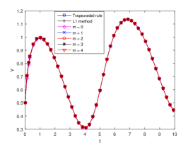
(a1) Case I.

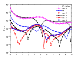
(a2) Case I.

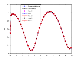
(b1) Case II.

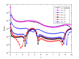
(b2) Case II.

Fig. 3: Numerical solutions and pointwise errors for Cases I and II, $\tau=T/2^{8}$, and $T=10$.

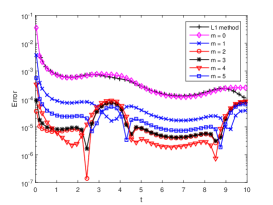
(a) $\sigma_{k}=\alpha_{1}+\alpha_{2}(k-1)$.

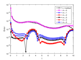
(b) $\sigma_{k}=0.1k$.

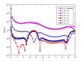
(c) $\sigma_{k}=0.15k$.

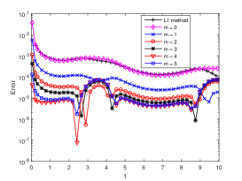
(d) $\sigma_{k}=0.2k$.

Fig. 4: Numerical solutions Pointwise errors for Case III, $\tau=T/2^{8}$, and $T=10$.

Example 5.3.

Consider the following fractional diffusion-wave equation

$$\left\{\begin{aligned} &\partial_{t}^{2}U+{}_{C}D^{1+\alpha}_{0,t}U=\partial_{x}^{2}U+f(x,t),{\quad}(x,t){\,\in\,}\Omega{\times}(0,1],\\ &U(x,0)=\sin(2\pi x),\quad\partial_{t}U(x,0)=\sin(2\pi x),{\quad}x{\,\in\,}\bar{\Omega},\\ &U(x,t)=0,{\quad}(x,t)\in\partial\Omega\times(0,1],\end{aligned}\right.$$ (41)

where $\Omega=(-1,1)$ and $0<\alpha<1$.

In this example, we consider two cases:

• Case I (Smooth solutions): Choose a suitable source term $f(x,t)$ such that the exact solution to (41) is $U(x,t)=(t^{4}+t^{3}+t^{2}+t+1)\sin(2\pi x).$

• Case II (Smooth inputs): The source term is $f=\exp(-t)\sin(\pi x)$, the initial conditions in (41) are replaced by $U(x,0)=\partial_{t}U(x,0)=0$, and $\alpha=1/2$.

We use the LGSEM (34)–(36) to solve (41), where the domain $\Omega$ is divided into three subdomains, i.e., $\Omega=(-1,-1/2]\cup[-1/2,1/2]\cup[1/2,1)$, and $N=(24,32,24)$.

In Table 11, we present the $L^{2}$ errors at $t=1$ for Case I (smooth solution with $\sigma_{k}=k$ in (22)). We choose $m_{1}=m_{2}=0$ and $m_{3}=0,1,2$ in the computation and observe that second-order accuracy is observed for $m_{3}=1,2$ and $\alpha=0.2,0.5,0.8,0.9$, which is in line with or even better than the theoretical analysis, see also Remark 4. However, for $m_{3}=0$, we do not obtain second-order accuracy, especially when $\alpha$ is close to 1; see also the related numerical results in [41, 45], where second-order accuracy was lost without correction terms.

For Case II, we do not have the explicit analytical solutions. It is known, see e.g. [9, p. 183] and [18, 19, 28], that the analytical solution of (41) satisfies $U(x,t)=c_{1}(x)t^{\sigma_{1}}+c_{2}(x)t^{\sigma_{2}}+c_{3}(x)t^{\sigma_{3}}+....$, where $\sigma_{k}=(3+k)\alpha,\,k=1,2,\ldots$ when $\alpha=1/2$. For simplicity, we choose $m_{1}=m_{2}=m_{3}=m$ in the computation. The benchmark solutions are obtained with smaller time step size $\tau=1/2048$. In Table 12, we present the $L^{2}$ errors at $t=1$ and observe second-order accuracy. Moreover, we find that more accurate numerical solutions are obtained when $m$ increases, which is in line with our theoretical predictions.

Table 11: The $L^{2}$ errors at $t=1$ for Case I, $N=(24,32,24)$, $m_{1}=m_{2}=0$.

$m_{3}$	$\tau$	$\alpha=0.2$	Order	$\alpha=0.5$	Order	$\alpha=0.8$	Order	$\alpha=0.9$	Order
	$2^{-5}$	2.6657e-4		6.1569e-4		1.7772e-3		2.4260e-3
	$2^{-6}$	6.7681e-5	1.97	1.8086e-4	1.76	6.9840e-4	1.34	1.0494e-3	1.20
0	$2^{-7}$	1.7203e-5	1.97	5.4727e-5	1.72	2.8484e-4	1.29	4.6837e-4	1.16
	$2^{-8}$	4.3805e-6	1.97	1.7044e-5	1.68	1.1915e-4	1.25	2.1310e-4	1.13
	$2^{-9}$	1.1178e-6	1.97	5.4503e-6	1.64	5.0648e-5	1.23	9.8050e-5	1.11
	$2^{-5}$	1.6225e-4		2.5548e-4		4.2711e-4		5.1769e-4
	$2^{-6}$	4.2531e-5	1.93	6.4545e-5	1.98	1.0434e-4	2.03	1.2298e-4	2.07
1	$2^{-7}$	1.0862e-5	1.96	1.6273e-5	1.98	2.6149e-5	1.99	3.0352e-5	2.01
	$2^{-8}$	2.7426e-6	1.98	4.0901e-6	1.99	6.6081e-6	1.98	7.6092e-6	1.99
	$2^{-9}$	6.8889e-7	1.99	1.0258e-6	1.99	1.6734e-6	1.98	1.9197e-6	1.98
	$2^{-5}$	2.5474e-4		4.6474e-4		8.2000e-4		9.9172e-4
	$2^{-6}$	6.2411e-5	2.02	1.1320e-4	2.03	1.9873e-4	2.04	2.4016e-4	2.04
2	$2^{-7}$	1.5464e-5	2.01	2.7927e-5	2.01	4.8842e-5	2.02	5.8955e-5	2.02
	$2^{-8}$	3.8497e-6	2.00	6.9349e-6	2.00	1.2104e-5	2.01	1.4598e-5	2.01
	$2^{-9}$	9.6047e-7	2.00	1.7279e-6	2.00	3.0125e-6	2.00	3.6316e-6	2.00

Table 12: The $L^{2}$ errors at $t=1$ for Case II, $N=(24,32,24)$, $\alpha=1/2$.

$\tau$	$m=0$	Order	$m=1$	Order	$m=2$	Order	$m=3$	Order
$2^{-5}$	2.6290e-4		1.7419e-4		3.0941e-5		5.0036e-5
$2^{-6}$	8.8199e-5	1.57	5.6954e-5	1.61	6.1603e-6	2.32	9.3685e-6	2.41
$2^{-7}$	3.0182e-5	1.54	1.9353e-5	1.55	1.3292e-6	2.21	1.8037e-6	2.37
$2^{-8}$	1.0260e-5	1.55	6.5824e-6	1.55	3.0150e-7	2.14	3.6715e-7	2.29
$2^{-9}$	3.3070e-6	1.63	2.1279e-6	1.62	6.8463e-8	2.13	7.7103e-8	2.25

6 Proofs

6.1 Proof of Lemma 1

A special case of Lemma 1 with $q=0,1$ and $\sigma$ being an integer can be found in [38]. We present the proof here for completeness and for all $q$.

Proof.

For $q=0$ and $U(t)=t^{\sigma}$, we have

$$\tau^{\alpha-\sigma}\mathcal{B}^{\alpha,n}_{0}U= \sum_{k=0}^{n}\omega^{(\alpha)}_{k}(n-k)^{\sigma}=\sum_{k=0}^{n}\omega^{(\alpha)}_{n-k}k^{\sigma}.$$ (42)

By analyzing the proof of Lemma 3.5 in [26] again, we can obtain

$$\sum_{k=0}^{n}\omega^{(\alpha)}_{n-k}k^{\sigma}=\frac{\Gamma(\sigma+1)}{\Gamma(\sigma+1-\alpha)}n^{\sigma-\alpha}-\frac{\alpha}{2}\frac{\Gamma(\sigma+1)}{\Gamma(\sigma-\alpha)}n^{\sigma-\alpha-1}+O(n^{\sigma-\alpha-2}),$$ (43)

which yields (5) for $q=0$. Now we prove (5) for $q\neq 0$. From (43), we have

$$\tau^{\alpha-\sigma}\mathcal{B}^{\alpha,n}_{q}U=\sum_{k=0}^{n+q}\omega^{(\alpha)}_{k}U(t_{n-k+q})=\sum_{k=0}^{n+q}\omega^{(\alpha)}_{k}(n-k+q)^{\sigma}$$ (44)

$$= \frac{\Gamma(\sigma+1)}{\Gamma(\sigma+1-\alpha)}(n+q)^{\sigma-\alpha}-\frac{\alpha}{2}\frac{\Gamma(\sigma+1)}{\Gamma(\sigma-\alpha)}(n+q)^{\sigma-\alpha-1}+O((n+q)^{\sigma-\alpha-2}).$$

By the fact that $\left(1+{q}/{n}\right)^{\sigma}=1+{\sigma}qn^{-1}+O(n^{-2}),n\geq|q|$, we have

$$\sum_{k=0}^{n+q}\omega^{(\alpha)}_{k}(n-k+q)^{\sigma} = \frac{\Gamma(\sigma+1)}{\Gamma(\sigma+1-\alpha)}\left(n^{\sigma-\alpha}+{(\sigma-\alpha)}qn^{\sigma-\alpha-1}\right)$$

$$-\frac{\alpha}{2}\frac{\Gamma(\sigma+1)}{\Gamma(\sigma-\alpha)}n^{\sigma-\alpha-1}+O(n^{\sigma-\alpha-2})$$

$$= \frac{\Gamma(\sigma+1)}{\Gamma(\sigma+1-\alpha)}n^{\sigma-\alpha}+\left(q-\frac{\alpha}{2}\right)\frac{\Gamma(\sigma+1)}{\Gamma(\sigma-\alpha)}n^{\sigma-\alpha-1}+O(n^{\sigma-\alpha-2}).$$

From (43) and (6.1), we reach (5), which completes the proof. ∎

6.2 Proof of Lemma 2

To prove Lemma 2, we need the following lemma.

Lemma 8.

Let $m$ be a positive integer and $w_{n,r}^{(\alpha)}\,(r=1,2,...,m)$ be defined by (10). Suppose that $\{\sigma_{r}\}$ are a sequence of strictly increasing positive numbers. Then we have

$$w_{n,r}^{(\alpha)}=O(n^{\sigma_{1}-2-\alpha})+O(n^{\sigma_{2}-2-\alpha})+\cdots+O(n^{\sigma_{m}-2-\alpha}).$$ (46)

Proof.

Letting $U(t)=t^{\sigma_{r}}$ and $(p,q)=(0,-1)$ in (8), we derive

$$\frac{\Gamma(\sigma_{r}+1)}{\Gamma(\sigma_{r}+1-\alpha)}n^{\sigma_{r}-\alpha}=\sum_{k=0}^{n}g^{(\alpha)}_{k}(n-k)^{\sigma_{r}}+O({n}^{\sigma_{r}-2-\alpha}).$$ (47)

Combining (47) and (10) yields a linear system

$$w_{n,1}^{(\alpha)} +2^{\sigma_{r}}w_{n,2}^{(\alpha)}+...+m^{\sigma_{r}}w_{n,m}^{(\alpha)}=O(n^{\sigma_{r}-2-\alpha}),{\quad}r=1,2,...,m,$$ (48)

which leads to (46). The proof is completed. ∎

Proof of Lemma 2.

Proof.

We have $\left[{}_{RL}D_{0,t}^{\alpha}U(t)\right]_{t=t_{n}}=\mathcal{A}_{p,q}^{\alpha,n,m}U+\tau^{\sigma-\alpha}H^{n,m,\alpha}(\sigma)$ from (5) and (8), and $H^{n,m,\alpha}(\sigma)$ satisfies (see Lemma 8)

$$H^{n,m,\alpha}(\sigma)= \frac{\Gamma(\sigma+1)}{\Gamma(\sigma+1-\alpha)}n^{\sigma-\alpha}-\sum_{k=0}^{n}g^{(\alpha)}_{k}(n-k)^{\sigma}-\sum_{k=1}^{m}w_{n,k}^{(\alpha)}k^{\sigma}$$

$$= Gn^{\sigma-\alpha-2}-\sum_{k=1}^{m}G_{k}n^{\sigma_{k}-\alpha-2}+{H}_{2}^{n,m,\alpha}(\sigma)={H}_{1}^{n,m,\alpha}(\sigma)+{H}_{2}^{n,m,\alpha}(\sigma),$$

where $G$ is independent of $n,\tau$, and $\sigma_{k}(1\leq k\leq m)$, $G_{k}$ is independent of $n$ and $\tau$, and ${H}_{2}^{n,m,\alpha}(\sigma)=O({n}^{\sigma-3-\alpha})+O({n}^{\sigma_{1}-3-\alpha})+\cdots+O({n}^{\sigma_{m}-3-\alpha})$. From Eqs. (3.1) and (3.13) in [26], we can readily obtain both $G$ and $G_{k}$ are analytical functions with respect to $\sigma$. Hence, $|\partial_{\sigma}^{r}G_{k}|$ and $|\partial_{\sigma}^{r}G|$ are bounded for a given $r$. Next, we derive a bound for ${H}_{1}^{n,m,\alpha}(\sigma)$. Since $H^{n,m,\alpha}(\sigma_{k})=0$, it implies ${H}_{1}^{n,m,\alpha}(\sigma_{k})=0$, $1\leq k\leq m$. It is known that ${H}_{1}^{n,m,\alpha}(\sigma)$ is infinitely smooth with respect to $\sigma$ and ${H}_{1}^{n,m,\alpha}(\sigma_{k})=0$, there exists an $\xi(\sigma)\in(\min\{\sigma,\sigma_{1},...,\sigma_{m}\},\max\{\sigma,\sigma_{1},...,\sigma_{m}\})$, such that

$${H}_{1}^{n,m,\alpha}(\sigma)=\frac{\partial_{\sigma}^{m}{H}_{1}^{n,m,\alpha}(\xi(\sigma))}{m!}\prod_{k=1}^{m}(\sigma-\sigma_{k}).$$

From the boundedness of $|\partial_{\sigma}^{r}G_{k}|$, $|\partial_{\sigma}^{r}G|$ , and the following relation

$$|\partial_{\sigma}^{m}(Gn^{\sigma-\alpha-2})|= \bigg{|}\sum_{k=0}^{m}\binom{k}{m}(\partial_{\sigma}^{m-k}G)\,n^{\sigma-\alpha-2}\log^{k}(n)\bigg{|}\leq Cn^{\sigma-\alpha-2}\log^{m}(n),$$

we have $|\partial_{\sigma}^{m}{H}_{1}^{n,m,\alpha}(\sigma)|\leq C\left(n^{\sigma-\alpha-2}\log^{m}(n)+n^{\sigma_{\max}-\alpha-2}\right)$, which leads to

$$|{H}_{1}^{n,m,\alpha}(\sigma)|\leq CS_{m}^{\sigma}\left(n^{\sigma-\alpha-2}\log^{m}(n)+n^{\sigma_{\max}-\alpha-2}\right).$$

With the same reasoning, we can derive that ${H}_{2}^{n,m,\alpha,\sigma}$ also satisfies

$$|{H}_{2}^{n,m,\alpha}(\sigma)|\leq \widetilde{C}\left[S_{m}^{\sigma}\left(n^{\sigma-\alpha-3}\log^{m}(n)+n^{\sigma_{\max}-\alpha-3}\right)+{n}^{\sigma_{\max}-4-\alpha}\right]$$

$$\leq C\left[S_{m}^{\sigma}\left(n^{\sigma-\alpha-3}\log^{m}(n)+n^{\sigma_{\max}-\alpha-3}\right)+{n}^{\sigma_{\max}-3-d-\alpha}\right],$$

where $d$ is a positive integer and $C$ is independent of $n$. From the estimates of ${H}_{1}^{n,m,\alpha}(\sigma)$ and ${H}_{2}^{n,m,\alpha}(\sigma)$, we obtain the desired result. The proof is completed. ∎

6.3 Proofs of Theorems 3–5

We first introduce a lemma.

Lemma 9.

Suppose that $a(z)=\sum_{k=0}^{\infty}a_{k}z^{k}$, $b(z)=\sum_{k=0}^{\infty}b_{k}z^{k}$, $\alpha$ is real, and $0\leq\beta\leq 1$. If $\left|a_{k}\right|\leq Ck^{\alpha}$ and $a(z)\left(1+\frac{\beta}{2}-\frac{\beta}{2}z\right)^{-1}=b(z)$, then there exists a positive constant $C$ independent of $k$, such that $|b_{k}|\leq Ck^{\alpha}$.

Proof.

From $a(z)\left(1+\frac{\beta}{2}-\frac{\beta}{2}z\right)^{-1}=b(z)$, we have $b_{0}=a_{0}\left(1+\frac{\beta}{2}\right)^{-1}$ and $a_{k}=\left(1+\frac{\beta}{2}\right)b_{k}-\frac{\beta}{2}b_{k-1},k>0$, which leads to $b_{k}=\frac{\beta}{2+\beta}b_{k-1}+\frac{2}{2+\beta}a_{k}$. Since $a_{k}=O(k^{\alpha})$, there exist a positive constant $C_{1}$ independent of $k$ such that $|a_{k}|\leq C_{1}k^{\alpha}$. With the mathematical induction method and $C_{1}\leq C/2$, we complete the proof. ∎

From Lemma 9 and Lemma 3.3 in [47], one can derive the following corollary.

Corollary 10.

Assume that $0\leq\beta_{2}\leq 1$, $\alpha\leq 1$, and $\beta_{1}$ is real. If $a_{n}=O(n^{\alpha})$ and $(1-z)^{\beta_{1}}\left(1+\frac{\beta_{2}}{2}-\frac{\beta_{2}}{2}z\right)^{-1}=\sum_{k=0}^{\infty}\tilde{g}_{k}z^{k}$, then $\left|\sum_{k=0}^{n}\tilde{g}_{k}a_{n-k}\right|\leq Cn^{\alpha-\beta_{1}}$.

6.3.1 Proof of Theorem 3

Proof.

Following the similar idea in [27] (see also [45]), we derive that the method (16) is stable if $-\lambda\in\mathbb{S}$, where $\mathbb{S}$ is defined by $\mathbb{S}=\mathbb{C}\setminus\big{\{}\sum_{j=1}^{Q}\nu_{j}\tau^{-\alpha_{j}}g^{(\alpha_{j})}(z),|z|\leq 1,\tau>0\big{\}}$, in which $g^{(\alpha_{j})}(z)=(1-z)^{\alpha_{j}}\left(1+\frac{\alpha_{j}}{2}-\frac{\alpha_{j}}{2}z\right)$. Since $\text{Re}(g^{(\alpha_{j})}(z))\geq 0$ for all $|z|\leq 1,\tau>0$ and $0<\alpha_{j}\leq 1$, the region $\mathbb{S}$ contains the whole negative real line, i.e., the scheme (16) is stable for any $\tau>0$. This completes the proof. ∎

6.3.2 Proof of Theorem 4

Proof.

Let $e^{n}=Y(t_{n})-y^{n}$. Then we derive the error equation of (16) as

$$\sum_{j=1}^{Q}\frac{\nu_{j}}{\tau^{\alpha_{j}}}\left[\sum_{k=0}^{n}g^{(\alpha_{j})}_{n-k}e^{k}+\sum_{r=1}^{m_{j}}w^{(\alpha_{j})}_{n,r}e^{r}\right]=f(t_{n},Y(t_{n}))-f(t_{n},y^{n})+R^{n},$$ (49)

where $R^{n}=\sum_{j=1}^{Q}O(\tau^{2}t_{n}^{\sigma_{m_{j}+1}-2-\alpha_{j}})$ is defined in (15). By Lemma 3.4 in [46], Eq. (49) can be written in the following form

$$\nu_{1}e^{n}+\sum_{j=2}^{Q}{\nu_{j}}{\tau^{\alpha_{1}-\alpha_{j}}}\left[\sum_{k=0}^{n}G^{(j)}_{n-k}e^{k}+\sum_{r=1}^{m_{j}}\sum_{k=0}^{n}\tilde{g}_{n-k}w^{(\alpha_{j})}_{k,r}e^{r}\right]$$ (50)

$$= {\tau^{\alpha_{1}}}\sum_{k=0}^{n}\tilde{g}_{n-k}(f(t_{k},Y(t_{k}))-f(t_{k},y^{k}))-\nu_{1}\sum_{r=1}^{m_{1}}\sum_{k=0}^{n}\tilde{g}_{n-k}w^{(\alpha_{1})}_{k,r}e^{r}+\tilde{R}^{n},$$

where $\tilde{R}^{n}={\tau^{\alpha_{1}}}\sum_{k=0}^{n}\tilde{g}_{n-k}R^{k}$, and $\{\tilde{g}_{k}\}$ and $\{G^{(j)}_{k}\}$ are, respectively, the coefficients of the Taylor expansions of the functions $\tilde{g}(z)=(1-z)^{-\alpha_{1}}\left(1+\frac{\alpha_{1}}{2}-\frac{\alpha_{1}}{2}z\right)^{-1}$ and

$$G^{(j)}(z)=(1-z)^{-(\alpha_{1}-\alpha_{j})}\left(1+\frac{\alpha_{j}}{2}-\frac{\alpha_{j}}{2}z\right)\left(1+\frac{\alpha_{1}}{2}-\frac{\alpha_{1}}{2}z\right)^{-1}.$$

Assume that $f(t,Y)$ satisfies the uniform Lipschitz condition, i.e., there exists a positive constant $L$ such that $|f(t_{k},Y(t_{k}))-f(t_{k},y^{k})|\leq L|Y(t_{k})-y^{k}|=L|e^{k}|$. Hence, for small enough $\tau$, we have

$$|e^{n}|\leq C\sum_{j=2}^{Q}{\tau^{\alpha_{1}-\alpha_{j}}}\sum_{k=0}^{n-1}G^{(j)}_{n-k}|e^{k}|+C{\tau^{\alpha_{1}}}\sum_{k=0}^{n-1}\tilde{g}_{n-k}|e^{k}|+\rho^{n},$$ (51)

where $\rho^{n}=C\sum_{j=1}^{Q}\sum_{r=1}^{m_{j}}\tau^{\alpha_{1}-\alpha_{j}}\Big{|}\sum_{k=0}^{n}\tilde{g}_{n-k}w^{(\alpha_{j})}_{k,r}\Big{|}|e^{r}|+C|\tilde{R}^{n}|.$

It is known that $(1-z)^{\alpha}=\sum_{k=0}^{\infty}\omega_{k}^{(\alpha)}z^{k}$ with $\omega_{k}^{(\alpha)}=O(k^{-\alpha-1})$. It then follows from Corollary 10 that $G^{(j)}_{k}=O(k^{\alpha_{1}-\alpha_{j}-1})$ and $\tilde{g}_{k}=O(k^{\alpha_{1}-1})$. We can similarly obtain $|\sum_{k=0}^{n}\tilde{g}_{n-k}w^{(\alpha_{j})}_{k,r}|\leq Cn^{\sigma_{m_{j}}-2-\alpha_{j}+\alpha_{1}}$ and $|\tilde{R}^{n}|\leq C\tau^{2}\sum_{j=1}^{Q}t_{n}^{\sigma_{m_{j}+1}-2-\alpha_{j}+\alpha_{1}}$. Hence, $\rho^{n}\leq C\left(\sum_{k=0}^{\max_{1\leq j\leq Q}\{m_{j}\}}|e^{k}|+\sum_{j=1}^{Q}n^{\sigma_{m_{j}+1}-2-\alpha_{j}+\alpha_{1}}\tau^{\sigma_{m_{j}+1}-\alpha_{j}+\alpha_{1}}\right)$. Similar to the proof in [22, Lemma 3.4], we derive (17).

If $f(t,Y)$ satisfies the local Lipschitz condition with respect to $Y$, then we can also derive (17) by the mathematical induction method, which is omitted here, see [22]. This ends the proof. ∎

6.3.3 Proof of Theorem 5

We first introduce a lemma.

Lemma 11 ([41]).

Suppose that $-1<\alpha\leq 1$. Then we have

$$\sum_{n=0}^{K}\left(\sum_{k=0}^{n}g^{(\alpha)}_{k}v_{n-k}\right)v_{n}\geq 0,$$

where $\{v_{k}\}$ are real numbers and $g^{(\alpha)}_{k}$ is defined by (11).

Proof.

From (49), we have

$$\sum_{j=1}^{Q}\frac{\nu_{j}}{\tau^{\alpha_{j}}}\left[\sum_{k=0}^{n}g^{(\alpha_{j})}_{n-k}e^{k}+\sum_{r=1}^{m_{j}}w^{(\alpha_{j})}_{n,r}e^{r}\right]+e^{n}=R^{n},$$ (52)

where $|R^{n}|\leq C\tau^{2}\sum_{j=1}^{Q}t_{n}^{\sigma_{m_{j}+1}-2-\alpha_{j}}$ is defined in (15).

Multiplying $e^{n}$ on both sides of (52) and summing up $n$ from $1$ to $K$, one has

$$\sum_{j=1}^{Q}\frac{\nu_{j}}{\tau^{\alpha_{j}}}\left[\sum_{n=1}^{K}\sum_{k=1}^{n}g^{(\alpha_{j})}_{n-k}e^{k}e^{n}+\sum_{r=1}^{m_{j}}\sum_{n=1}^{K}w^{(\alpha_{j})}_{n,r}e^{r}e^{n}\right]+\sum_{n=1}^{K}|e^{n}|^{2}=\sum_{n=1}^{K}R^{n}e^{n}.$$ (53)

Applying Lemma 11 and the Cauchy–Schwarz inequality, we have

$$\sum_{n=1}^{K}|e^{n}|^{2}\leq\sum_{j=1}^{Q}\frac{\nu_{j}}{\tau^{\alpha_{j}}}\sum_{n=1}^{K}\sum_{k=1}^{n}g^{(\alpha_{j})}_{n-k}e^{k}e^{n}+\sum_{n=1}^{K}|e^{n}|^{2}$$ (54)

$$\leq \sum_{n=1}^{K}R^{n}e^{n}-\sum_{j=1}^{Q}\frac{\nu_{j}}{\tau^{\alpha_{j}}}\sum_{r=1}^{m_{j}}\sum_{n=1}^{K}w^{(\alpha_{j})}_{n,r}e^{r}e^{n}$$

$$\leq \frac{1}{2}\sum_{n=1}^{K}(|R^{n}|^{2}+|e^{n}|^{2})+\sum_{j=1}^{Q}\sum_{r=1}^{m_{j}}\sum_{n=1}^{K}\bigg{(}\frac{|w^{(\alpha_{j})}_{n,r}|^{2}\nu_{j}^{2}\tau^{-2\alpha_{j}}}{4\epsilon}|e^{r}|^{2}+\epsilon|e^{n}|^{2}\bigg{)},$$

where $\epsilon>0$ is a positive constant. If we choose $\epsilon=\frac{1}{4Q(m_{1}+m_{2}+...+m_{Q})}$, then we have

$$\sum_{n=1}^{K}|e^{n}|^{2} \leq C\sum_{n=1}^{K}|R^{n}|^{2}+C\sum_{j=1}^{Q}\sum_{r=1}^{m_{j}}\sum_{n=1}^{K}{\tau^{-2\alpha_{j}}|w^{(\alpha_{j})}_{n,r}|^{2}}|e^{r}|^{2}.$$ (55)

Let $q_{j}=\sigma_{m_{j}+1}-\alpha_{j}$. From (55), (46), and $|R^{n}|\leq C\tau^{2}\sum_{j=1}^{Q}t_{n}^{\sigma_{m_{j}+1}-2-\alpha_{j}}$, we have

$$\tau\sum_{n=1}^{K}|e^{n}|^{2} \leq C\tau\sum_{n=1}^{K}|R^{n}|^{2}+C\sum_{j=1}^{Q}\sum_{r=1}^{m_{j}}\sum_{n=1}^{K}{\tau^{1-2\alpha_{j}}|w^{(\alpha_{j})}_{n,r}|^{2}}|e^{r}|^{2}$$

$$\leq C\sum_{j=1}^{Q}\tau^{2q_{j}+1}\sum_{n=1}^{K}n^{2(q_{j}-2)}+C\max_{1\leq r\leq m}|e^{r}|^{2}\bigg{(}\sum_{j=1}^{Q}\tau^{1-2\alpha_{j}}\sum_{n=1}^{K}n^{{2(\sigma_{m}-\alpha_{j}-2)}}\bigg{)}$$

$$\leq C\sum_{j=1}^{Q}\bigg{(}\tau^{2q_{j}+1}K^{\max\{0,2q_{j}-3\}}+\max_{1\leq r\leq m}|e^{r}|^{2}\tau^{1-2\alpha_{j}}K^{\max\{0,2\sigma_{m}-2\alpha_{j}-3\}}\bigg{)}.$$

Let $q=\min_{1\leq j\leq Q}\{q_{j}\}$. Then we have from the above equation

$$\tau\sum_{n=1}^{K}|e^{n}|^{2} \leq C\tau^{\min\{4,2q+1\}}+C\max_{1\leq r\leq m}|e^{r}|^{2}\sum_{j=1}^{Q}\tau^{1-2\alpha_{j}}K^{\max\{0,2\sigma_{m}-2\alpha_{j}-3\}},$$

which leads to (18). The proof is completed. ∎

7 Summary

In this work, we obtained the asymptotic expansion of the error equation of the WSGL formula (7) proposed in [39]. The WSGL formula is second-order accurate far from $t=0$ but is not second-order accurate near $t=0$. Hence second-order numerical scheme is not expected when the formula is applied to time-fractional differential equations. We then followed Lubich’s approach by adding the correction terms to the WSGL formula and obtained a modified formula with global second-order accuracy both around and far from $t=0$. We applied our modified formula to solve two-term FODEs and two-term time-fractional anomalous diffusion equations and proved the stability and second-order convergence in time.

We found that only a small number of correction terms is needed to improve convergence order and accuracy regardless of regularity of the analytical solutions. We showed both theoretically and numerically that a few correction terms are sufficient to obtain relatively high accuracy at $t=0$ and thus improve the convergence order and accuracy far from $t=0$. With a few correction terms, we avoid solving the linear system with an exponential Vandermonde matrix of large size to obtain starting weights. We observed that with no more than $10$ terms, the linear system can be accurately solved with double precision without harming the accuracy of the second-order formula. Moreover, the correction terms do not have to exactly match the singularity indexes of solutions to FDEs. Even when we do not know the precise singularity indices of solutions to FDEs, we provided some empirical guidelines to choose correction terms.

Although, we only focus on the WSGL formulas, the methodology proposed here can be also applied to recover globally high accuracy for some other high-order formulas, see e.g. [4, 6, 12, 13, 17, 46, 52, 54], where the high-order accuracy requires vanishing initial/boundary values of the corresponding function, even vanishing values of higher-order derivatives at boundaries.

a Supplementary Material

We provide more numerical results to support the theoretical analysis and the proofs of Theorems 6–7 in Subsection 4.3.

a.1 Further investigation of the upper bound of (12)

Numerically, we find a much better upper bound of (12), which is presented below

$$|{R_{n}}|\leq C_{m}S_{m}^{\sigma}\tau^{\sigma-\alpha-2}n^{\max\{\sigma_{\max},\sigma\}-\alpha-2}.$$ (56)

We plot a bound of $C_{m}$ in (56) for $U(t)=t^{0.85}$, which is shown in Fig. 5. We see that $C_{m}$ does not increase with respect to $m$ and $\alpha$.

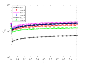
(a) $\alpha=0.06$.

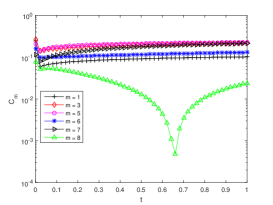
(b) $\alpha=0.1$.

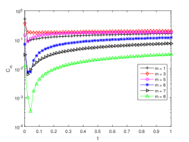
(c) $\alpha=0.2$.

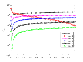
(d) $\alpha=0.3$.

Fig. 5: The bound of constant $C_{m}$ in (56), $U(t)=t^{0.85}$, $\tau=10^{-3}$.

a.2 More numerical results for multi-term FODEs

We present an example using more than ten correction terms to solve the following FODE.

Example a.1.

Consider the following two-term FODE

$${}_{C}D^{2\alpha}_{0,t}Y(t)+{}_{C}D^{\alpha}_{0,t}Y(t)=-Y(t)+f(t),{\quad}t{\,\in\,}{(0,T],T>0}\\$$ (57)

subject to the initial condition $Y(0)=1$, and $0<\alpha\leq 1/2$.

Choose a suitable right-hand side function $f(t)$ such that the analytical solution of (57) is

$$Y(t)=1+\sum_{k=1}^{16}\frac{t^{(k+1)\alpha}}{k}.$$

Here, we use the multi-precision toolbox with 48 significant digits in the computation in order to avoid round-off errors (see http://www.mathworks.com/matlabcentral /fileexchange/6446-multiple-precision-toolbox-for-matlab).

We consider only the fractional order $\alpha=0.05,0.1$ with $\sigma_{k}=(k+1)\alpha$ in (16), and the pointwise errors are shown in Figs. 6–7. We can see that very accurate numerical solutions are obtained as the number of correction terms increases. Although we did not observe the global second-order accuracy, the small factor $S_{m}^{\sigma}$ in the error equation makes numerical solutions very accurate as correction terms increases.

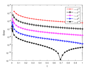
(a) $m=10$.

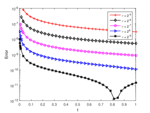
(b) $m=12$.

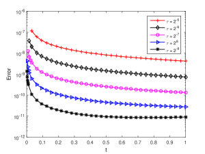
(c) $m=14$.

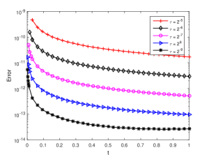
(d) $m=15$.

Fig. 6: Pointwise errors of Example a.1, $\alpha=0.1$.

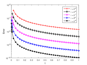
(a) $m=10$.

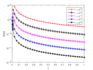
(b) $m=12$.

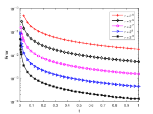
(c) $m=14$.

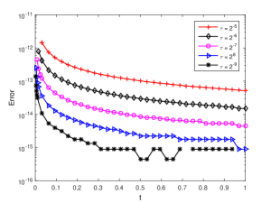
(d) $m=15$.

Fig. 7: Pointwise errors of Example a.1, $\alpha=0.05$.

a.3 Proofs of Theorems 6 and 7

We prove the stability and convergence analysis of LGSEM (34)–(36). We first introduce a lemma.

Lemma 12 (Gronwall’s inequality [35]).

Suppose that $\{k_{n}\}$, $\{\phi_{n}\}$ and $\{p_{n}\}$ are nonnegative sequence. Let $A\geq 0$ and $\phi_{n}$ satisfies

$$\phi_{n}\leq A+\sum_{j=0}^{n-1}p_{j}+\sum_{j=0}^{n-1}k_{j}\phi_{j},{\quad}n\geq 0.$$

Then we have $\phi_{n}\leq\left(A+\sum_{j=0}^{n-1}p_{j}\right)\exp\left(\sum_{j=0}^{n-1}k_{j}\right).$

a.3.1 Proof of Theorem 6

Proof.

Letting $v=2\tau v_{N}^{n+\frac{1}{2}}$ in (34) and $u=2\mu\tau u_{N}^{n+\frac{1}{2}}$ in (35), and eliminating the intermediate term $2\mu\tau\,(\partial_{x}u_{N}^{n+\frac{1}{2}},\partial_{x}v_{N}^{n+\frac{1}{2}})$, we obtain

$$\|v_{N}^{n+1}\|^{2}-\|v_{N}^{n}\|^{2}+2{\nu}\tau^{1-\alpha}\sum_{k=0}^{n}g^{(\alpha)}_{k}(v_{N}^{n-k+\frac{1}{2}},v_{N}^{n+\frac{1}{2}})+\mu(\|\partial_{x}u_{N}^{n+1}\|^{2}-\|\partial_{x}u_{N}^{n}\|^{2})$$ (58)

$$= 2{\nu}\tau^{1-\alpha}\bigg{[}C_{n}(v_{N}^{0},v_{N}^{n+\frac{1}{2}})-\sum_{r=1}^{m_{3}}W_{n,r}(v_{N}^{r}-v_{N}^{0},v_{N}^{n+\frac{1}{2}})\bigg{]}-\sum_{r=1}^{m_{2}}v_{n,r}(v_{N}^{r}-v_{N}^{0},v_{N}^{n+\frac{1}{2}})$$

$$-2\mu\sum_{r=1}^{m_{1}}u_{n,r}(\partial_{x}(u_{N}^{r}-u_{N}^{0}-t_{r}v_{N}^{0}),\partial_{x}u_{N}^{n+\frac{1}{2}})+2\tau(I_{N}f^{n+\frac{1}{2}},v_{N}^{n+\frac{1}{2}}),$$

where $C_{n}$ and $W_{n,r}(r=1,2)$ are defined by

$$C_{n} = \sum_{k=0}^{n}g^{(\alpha)}_{k}=O(n^{-\alpha}),$$ (59)

$$W_{n,r} = \frac{1}{2}(w_{n,r}^{(\alpha)}+w_{n+1,r}^{(\alpha)}),$$ (60)

in which $\{w_{n,r}^{(\alpha)}\}$ are defined by (10) with $\sigma_{r}$ replaced by $\sigma_{r}-1$. Here $C_{n}=O(n^{-\alpha})$ can be derived from the fact $\sum_{k=0}^{n}\omega^{(\alpha)}_{k}=O(n^{-\alpha})$ (see Lemma 3.4 in [47]) and the definition of $g^{(\alpha)}_{k}$ (see (11)). Also, $|W_{n,r}|\leq Cn^{\sigma_{m_{3}}-3-\alpha}$ can be derived from Lemma 8 with $\sigma_{m}=\sigma_{m_{3}}-1$ in (46).

Summing up $n$ from 0 to $K$ and applying Lemma 11, we obtain

$$\|v_{N}^{K+1}\|^{2} + \mu\|\partial_{x}u_{N}^{K+1}\|^{2}\leq\|v_{N}^{0}\|^{2}+\mu\|\partial_{x}u_{N}^{0}\|^{2}+2\tau\sum_{n=0}^{K}(I_{N}f^{n+\frac{1}{2}},v_{N}^{n+\frac{1}{2}})$$ (61)

$$+2{\nu}\tau^{1-\alpha}\sum_{n=0}^{K}C_{n}(v_{N}^{0},v_{N}^{n+\frac{1}{2}})-2{\nu}\tau^{2-\alpha}\sum_{n=0}^{K}\sum_{r=1}^{m_{3}}W_{n,r}\left((v_{N}^{r}-v_{N}^{0})/\tau,v_{N}^{n+\frac{1}{2}}\right)$$

$$-\tau\sum_{n=0}^{K}\sum_{r=1}^{m_{2}}v_{n,r}\left((v_{N}^{r}-v_{N}^{0})/\tau,v_{N}^{n+\frac{1}{2}}\right)$$

$$-2\mu\tau\sum_{n=0}^{K}\sum_{r=1}^{m_{1}}u_{n,r}\left(\partial_{x}(u_{N}^{r}-u_{N}^{0})/\tau-r\partial_{x}v_{N}^{0},\partial_{x}u_{N}^{n+\frac{1}{2}}\right).$$

Applying the Cauchy–Schwarz inequality yields

$$\|v_{N}^{K+1}\|^{2}+\mu\|\partial_{x}u_{N}^{K+1}\|^{2}\leq\|v_{N}^{0}\|^{2}+\mu\|\partial_{x}u_{N}^{0}\|^{2}+C\tau\sum_{n=0}^{K}\left(\|f^{n+\frac{1}{2}}\|^{2}+\|v_{N}^{n+\frac{1}{2}}\|^{2}\right)$$

$$+C\tau^{1-\alpha}\sum_{n=0}^{K}\left[|C_{n}|\left(\|v_{N}^{0}\|^{2}+\|v_{N}^{n+\frac{1}{2}}\|^{2}\right)+\tau\sum_{r=1}^{m_{3}}|W_{n,r}|\left(\|(v_{N}^{r}-v_{N}^{0})/\tau\|^{2}+\|v_{N}^{n+\frac{1}{2}}\|^{2}\right)\right]$$

$$+C\tau\sum_{n=0}^{K}\sum_{r=1}^{m_{2}}|v_{n,r}|\left(\|(v_{N}^{r}-v_{N}^{0})/\tau\|^{2}+\|v_{N}^{n+\frac{1}{2}}\|^{2}\right)$$

$$+C\tau\sum_{n=0}^{K}\sum_{r=1}^{m_{1}}|u_{n,r}|\left(\|\partial_{x}(u_{N}^{r}-u_{N}^{0})/\tau\|^{2}+\|\partial_{x}v_{N}^{0}\|^{2}+\|\partial_{x}u_{N}^{n+\frac{1}{2}}\|^{2}\right),$$ (62)

where $C$ is a positive constant independent of $\tau,h,n,k$ and $K$. For simplicity, we denote

$$S_{1}^{K}=\sum_{n=1}^{K}n^{\sigma_{m_{1}}-3},{\quad}S_{2}^{K}=\sum_{n=1}^{K}n^{\sigma_{m_{2}}-4},{\quad}S_{3}^{K}=\sum_{n=1}^{K}n^{\sigma_{m_{3}}-3-\alpha}.$$ (63)

Then we obtain

$$S_{1}^{K}= \sum_{n=1}^{K}n^{\sigma_{m_{1}}-3}\leq C\max\{1,K^{\sigma_{m_{1}}-2}\},{\quad}S_{2}^{K}=\sum_{n=1}^{K}n^{\sigma_{m_{2}}-4}\leq C\max\{1,K^{\sigma_{m_{2}}-3}\},$$ (64)

$$S_{3}^{K}= \sum_{n=1}^{K}n^{\sigma_{m_{3}}-3-\alpha}\leq C\max\{1,K^{\sigma_{m_{3}}-2-\alpha}\}.$$

Note from (59), (60), and Lemma 8 that

$$|W_{n,r}| \leq Cn^{\sigma_{m_{3}}-3-\alpha},\,|v_{n,r}|\leq Cn^{\sigma_{m_{2}}-4},\,|u_{n,r}|\leq Cn^{\sigma_{m_{1}}-3},\,C_{n}=O(n^{-\alpha}).$$ (65)

Hence, we derive from (62)–(64)

$$\|v_{N}^{K+1}\|^{2}+\mu\|\partial_{x}u_{N}^{K+1}\|^{2}\leq C(\|v_{N}^{0}\|^{2}+\mu\|\partial_{x}u_{N}^{0}\|^{2}+\|\partial_{x}v_{N}^{0}\|^{2})$$

$$+C\sum_{n=1}^{K+1}\Big{(}\tau^{1-\alpha}n^{-\alpha}+\tau+\tau^{2-\alpha}n^{\sigma_{m_{3}}-3-\alpha}+\tau n^{\sigma_{m_{2}}-4}\Big{)}\|v_{N}^{n}\|^{2}$$

$$+C\tau\sum_{n=1}^{K+1}n^{\sigma_{m_{1}}-3}\|\partial_{x}u_{N}^{n}\|^{2}+C\tau^{1-\alpha}\|v_{N}^{0}\|^{2}\sum_{n=0}^{K}|C_{n}|+C\tau\sum_{n=0}^{K+1}\|f^{n}\|^{2}$$

$$+C\tau\sum_{r=1}^{m_{2}}\|\delta_{t}v_{N}^{r-\frac{1}{2}}\|^{2}S_{2}^{K}+C\tau^{2-\alpha}\sum_{r=1}^{m_{3}}\|\delta_{t}v_{N}^{r-\frac{1}{2}}\|^{2}S_{3}^{K}+C\tau\sum_{r=1}^{m_{1}}\|\partial_{x}\delta_{t}u_{N}^{r-\frac{1}{2}}\|^{2}S_{1}^{K}.$$

For small enough $\tau$, using the assumption $\sigma_{m_{1}}\leq 3$, $\sigma_{m_{2}},\sigma_{m_{3}}\leq 4$, and (64), we can get from the above inequality

$$\|v_{N}^{K+1}\|^{2}+\mu\|\partial_{x}u_{N}^{K+1}\|^{2}\leq\rho^{K}+C\sum_{n=1}^{K}d_{n}(\|v_{N}^{n}\|^{2}+\mu\|\partial_{x}u_{N}^{n}\|^{2}),$$ (66)

where $d_{n}=\tau^{1-\alpha}n^{-\alpha}+\tau+\tau^{2-\alpha}n^{\sigma_{m_{3}}-3-\alpha}+\tau n^{\sigma_{m_{2}}-4}+\tau n^{\sigma_{m_{1}}-3}$, and

$$\rho^{K}= C\bigg{(}\|v_{N}^{0}\|^{2}+\mu\|\partial_{x}u_{N}^{0}\|^{2}+\|\partial_{x}v_{N}^{0}\|^{2}+\tau\sum_{r=1}^{m_{1}}\|\partial_{x}\delta_{t}u_{N}^{r-\frac{1}{2}}\|^{2}S_{1}^{K}$$ (67)

$$+\tau\sum_{r=1}^{m_{2}}\|\delta_{t}v_{N}^{r-\frac{1}{2}}\|^{2}S_{2}^{K}+\tau^{2-\alpha}\sum_{r=1}^{m_{3}}\|\delta_{t}v_{N}^{r-\frac{1}{2}}\|^{2}S_{3}^{K}+\tau\sum_{n=0}^{K+1}\|f^{n}\|^{2}\bigg{)}.$$

Applying Gronwall’s inequality (Lemma 12) yields

$$\|v_{N}^{K+1}\|^{2}+\mu\|\partial_{x}u_{N}^{K+1}\|^{2}\leq\rho^{K}\exp\left(C\sum_{n=1}^{K}d_{n}\right).$$ (68)

Using the condition $\sigma_{m_{1}}\leq 3$ and $\sigma_{m_{2}},\sigma_{m_{3}}\leq 4$ leads to

$$\sum_{n=1}^{K}d_{n}\leq C(T^{1-\alpha}+T^{2-\alpha}+T+1).$$ (69)

Applying (64), $\sigma_{m_{1}}\leq 3$ and $\sigma_{m_{2}},\sigma_{m_{3}}\leq 4$ yields

$$\rho^{K} \leq C(\|v_{N}^{0}\|^{2}+\mu\|\partial_{x}u_{N}^{0}\|^{2}+\|\partial_{x}v_{N}^{0}\|^{2})+C\sum_{r=1}^{m_{1}}\|\partial_{x}\delta_{t}u_{N}^{r-\frac{1}{2}}\|^{2}$$ (70)

$$+C\sum_{r=1}^{m_{2}}\|\delta_{t}v_{N}^{r-\frac{1}{2}}\|^{2}+C\sum_{r=1}^{m_{3}}\|\delta_{t}v_{N}^{r-\frac{1}{2}}\|^{2}+C\tau\sum_{n=0}^{K+1}\|f^{n}\|^{2}.$$

Combining (68)–(70) reaches the conclusion. This completes the proof. ∎

a.3.2 Proof of Theorem 7

We now focus on the convergence of the scheme (34)–(36). Introduce the projector $P_{N}^{1,0}$: $H^{1}_{0}(\Omega)\to V_{N}^{0}$ as

$$(\partial_{x}(P_{N}^{1,0}u-u),\partial_{x}v)=0,{\quad}u\in H^{1}_{0}(\Omega),{\quad}\forall v\in V_{N}^{0}.$$ (71)

The properties of the interpolation and projection operators are listed below.

Lemma 13 ([2]).

If $u{\,\in\,}{H^{r}(\Omega)},\,r{\,\geq\,}0$, then we have

$$\big{\|}{\partial_{x}^{l}(u-I_{N}u)}\big{\|}{\leq}Ch^{r-l}\|{u}\|_{H^{r}(\Omega)},{\quad}l=0,1.$$

Lemma 14 ([2]).

If $u{\,\in\,}{H^{r}(\Omega)}\cap{H^{1}_{0}(\Omega)},\,r{\,\geq\,}1$, then

$$\big{\|}{\partial_{x}^{l}(u-P_{N}^{1,0}u)}\big{\|}{\leq}Ch^{r-l}\|{u}\|_{H^{r}(\Omega)},{\quad}l=0,1.$$

Denote by $e_{u}=u_{N}-P_{N}^{1,0}U$, $\eta_{u}=U-P_{N}^{1,0}U$, $e_{v}=v_{N}-P_{N}^{1,0}V$, and $\eta_{v}=V-P_{N}^{1,0}V$. Then we get the error equation of (34)–(36) as follows

$$(\delta_{t}e_{v}^{n+\frac{1}{2}},v)+\frac{1}{\tau}\sum_{r=1}^{m_{2}}v_{n,r}(e_{v}^{r}-e_{v}^{0},v)+\frac{\nu}{2}\left[\left(\mathcal{{A}}_{0,-1}^{\alpha,n+1,m_{3}}(e_{v}-e_{v}^{0}),v\right)+\left(\mathcal{{A}}_{0,-1}^{\alpha,n,m_{3}}(e_{v}-e_{v}^{0}),v\right)\right]$$

$${\qquad\qquad\quad}+\mu\,(\partial_{x}e_{u}^{n+\frac{1}{2}},\partial_{x}v)=(G^{n},v),$$ (72)

$$(\delta_{t}\partial_{x}e_{u}^{n+\frac{1}{2}},\partial_{x}u)+\frac{1}{\tau}\sum_{r=1}^{m_{1}}u_{n,r}(\partial_{x}(e_{u}^{r}-e_{u}^{0}-t_{r}e_{v}^{0}),v)-(\partial_{x}e_{v}^{n+\frac{1}{2}},\partial_{x}u)=(H^{n},u),$$ (73)

where $u,v\in V_{N}^{0}$, $H^{n}=O(\tau^{2}t_{n}^{\sigma_{m_{1}+1}-3})$, and

$$G^{n} = \delta_{t}\eta_{v}^{n+\frac{1}{2}}+\frac{1}{\tau}\sum_{r=1}^{m_{2}}v_{n,r}(\eta_{v}^{r}-\eta_{v}^{0})+\frac{\nu}{2}\left(\mathcal{{A}}_{0,-1}^{\alpha,n+1,m_{3}}(\eta_{v}-\eta_{v}^{0})+\mathcal{{A}}_{0,-1}^{\alpha,n,m_{3}}(\eta_{v}-\eta_{v}^{0})\right)$$

$$+I_{N}f^{n+1}-f^{n+1}+O(\tau^{2}t_{n}^{\sigma_{m_{2}+1}-4})+O(\tau^{2}t_{n}^{\sigma_{m_{3}+1}-3-\alpha}).$$

Proof.

From Theorem 6, (72)–(73), and the properties $e_{v}^{0}=e_{u}^{0}=0$, we can similarly derive

$$\|e_{v}^{n}\|^{2}+\mu\|\partial_{x}e_{u}^{n}\|^{2}\leq CR^{m_{1},m_{2},m_{3}}(e)+C\tau\sum_{k=0}^{n}\left(\|G^{k}\|^{2}+\|H^{k}\|^{2}\right),$$ (74)

where

$$R^{m_{1},m_{2},m_{3}}(e)=\sum_{k=1}^{m_{1}}\|\partial_{x}\delta_{t}e_{u}^{k-\frac{1}{2}}\|^{2}+\sum_{k=1}^{m_{2}}\|\delta_{t}e_{v}^{k-\frac{1}{2}}\|^{2}+\sum_{k=1}^{m_{3}}\|\delta_{t}e_{v}^{k-\frac{1}{2}}\|^{2}.$$

It is easy to obtain $\|H^{n}\|\leq Cn^{\sigma_{m_{1}+1}-3}\tau^{\sigma_{m_{1}+1}-1}$ and

$$\|G^{n}\|\leq C\left(h^{r}+n^{\sigma_{m_{2}+1}-4}\tau^{\sigma_{m_{2}+1}-2}+n^{\sigma_{m_{3}+1}-3-\alpha}\tau^{\sigma_{m_{3}+1}-1-\alpha}\right).$$

From (74) and the boundedness of $\|G^{n}\|$ and $\|H^{n}\|$, we derive

$$\|e_{v}^{n}\|^{2} + \mu\|\partial_{x}e_{u}^{n}\|^{2}\leq C\bigg{(}h^{2r}+R^{m_{1},m_{2},m_{3}}(e)+\tau^{2\sigma_{m_{1}+1}-1}\sum_{k=1}^{n}k^{2(\sigma_{m_{1}+1}-3)}$$ (75)

$$+\tau^{2\sigma_{m_{2}+1}-3}\sum_{k=1}^{n}k^{2(\sigma_{m_{2}+1}-4)}+\tau^{2\sigma_{m_{3}+1}-1-2\alpha}\sum_{k=1}^{n}k^{2(\sigma_{m_{2}+1}-3-\alpha)}\bigg{)}.$$

Using the assumption $\sigma_{m_{1}}\leq 3,\sigma_{m_{2}},\sigma_{m_{3}}\leq 4$ and applying the property $\sum_{k=1}^{n}k^{\beta}\leq C\max\{1,n^{1+\beta}\},\beta\in\mathbb{R},\beta\neq-1$, we obtain

$$\|e_{v}^{n}\|^{2} +\mu\|\partial_{x}e_{u}^{n}\|^{2}\leq C\Big{(}h^{2r}+R^{m_{1},m_{2},m_{3}}(e)+\tau^{\min\{4,2{\sigma_{m_{1}+1}-1},2\sigma_{m_{2}+1}-3,2\sigma_{m_{3}+1}-1-2\alpha\}}\Big{)}.$$

We can get $R^{m_{1},m_{2},m_{3}}(e)\leq C(h^{2r-2}+\tau^{\min\{4,2{\sigma_{m_{1}+1}-1},2\sigma_{m_{2}+1}-3,2\sigma_{m_{3}+1}-1-2\alpha\}})$ from the assumption, hence

$$\max\{\|e_{v}^{n}\|,\|\partial_{x}e_{u}^{n}\|\}\leq C\Big{(}\tau^{\min\{2,{\sigma_{m_{1}+1}-0.5},\sigma_{m_{2}+1}-1.5,\sigma_{m_{3}+1}-0.5-\alpha\}}+h^{r-1}\Big{)}.$$

Applying the triangle inequality $\|\partial_{x}(u_{N}^{n}-U(t_{n}))\|\leq\|\partial_{x}e_{u}^{n}\|+\|\partial_{x}\eta_{u}^{n}\|$ and Lemma 14 yields the desired result. ∎

a.4 Multi-term time-fractional subdiffusion equation

Consider the following multi-term time-fractional subdiffusion equation

$$\left\{\begin{aligned} &{}_{C}D^{\alpha_{1}}_{0,t}U+\nu\,{}_{C}D^{\alpha_{2}}_{0,t}U=\mu\,\partial_{x}^{2}U+f(x,t),{\quad}(x,t){\,\in\,}\Omega{\times}(0,T],T>0,\\ &U(x,0)=\phi_{0}(x),{\quad}x{\,\in\,}\bar{\Omega},\\ &U(x,t)=0,{\quad}(x,t)\in\partial\Omega\times(0,T],\end{aligned}\right.$$ (76)

where $\Omega=(a,b)$, $0<\alpha_{1},\alpha_{2}\leq 1$, $\nu\geq 0$, and $\mu>0$. Here, we extend LGSEM (34)–(36) to solve (76), which can be easily extended to more generalized multi-term time-fractional subdiffusion equations, see e.g. [20, 25, 37]. We directly present the LGSEM for (76) as: Find $u_{N}^{n}\in V_{N}^{0}$ for $n=1,2,...,n_{T}$, such that

$$\left(\mathcal{{A}}_{0,-1}^{{\alpha_{1}},n,m_{1}}\hat{u}_{N},v\right)+\nu\left(\mathcal{{A}}_{0,-1}^{{\alpha_{2}},n,m_{2}}\hat{u}_{N},v\right)+\mu(\partial_{x}u_{N}^{n},\partial_{x}v)=(I_{N}f^{n},v),\,\,\forall v\in V_{N}^{0},$$ (77)

$$u_{N}^{0}=P_{N}^{1,0}U(0).$$ (78)

where $\hat{u}_{N}^{k}=u_{N}^{k}-u_{N}^{0}\,(k\geq 0)$, $m_{1},m_{2}$ are suitable positive integers, and $\mathcal{{A}}_{0,-1}^{\alpha_{k},n,m_{k}}\,(k=1,2)$ are defined as in (9).

The convergence of the scheme (77)–(78) can be similarly proven as that of Theorem 7, which is given by

$$\left(\tau\sum_{k=0}^{n}\|\partial_{x}(u_{N}^{k}-U(t_{k}))\|^{2}\right)^{1/2}\leq C\left(\tau^{\min\{2,\sigma_{m_{1}+1}-{\alpha_{1}},\sigma_{m_{2}+1}-{\alpha_{2}}\}}+h^{r-1}\right),$$

where the analytical solution of (76) satisfies $U(t)-U(0)=\sum_{r=1}^{m}c_{r}t^{\sigma_{r}}+u(t)t^{\sigma_{m+1}}$, $u(t)$ is uniformly bounded for $t\in[0,T]$, $U(t)\in H_{0}^{r}(\Omega)$, and $\sigma_{m_{1}},\sigma_{m_{2}}\leq 3$.

Remark 6.

If $m_{1}=m_{2}=0$ in (77)–(78), then we have

$$\|\partial_{x}(u_{N}^{n}-U(t_{n}))\| \leq C\left(\tau^{\min\{2,\sigma_{1}-{\alpha_{1}},\sigma_{1}-{\alpha_{2}}\}}+h^{r-1}\right),$$

$$\left(\tau\sum_{k=0}^{n}\|\partial_{x}(u_{N}^{k}-U(t_{k}))\|^{2}\right)^{1/2} \leq C\left(\tau^{\min\{2,\sigma_{1}-{\alpha_{1}}+0.5,\sigma_{1}-{\alpha_{2}}+0.5\}}+h^{r-1}\right).$$

Example a.2.

Consider the following time-fractional subdiffusion equation

$${}_{C}D^{\alpha_{1}}_{0,t}U+{}_{C}D^{\alpha_{2}}_{0,t}U=\partial_{x}^{2}U+\exp(-t){\sin(\pi x)},{\quad}(x,t){\,\in\,}(0,1){\times}(0,T],T>0$$ (79)

subject to the homogenous initial and boundary conditions, $\alpha_{1}=3/4$, and $\alpha_{2}=1/2$.

Next, we use the scheme (77)–(78) with $m_{1}=m_{2}=m$ to solve (79). Here in space, we use two subdomains: $[0,1]=[0,1/2]\cup[1/2,1]$, and $N=(32,32)$. We observe numerically that the resolution in space is fine enough and the total error is dominated by errors from time discretization.

It is known in [9, p. 183] that the analytical solution $U(t)$ to (79) satisfies $U(t)=\sum_{k=1}^{\infty}c_{k}t^{\sigma_{k}}$, where $\sigma_{k}=(2+k)/4$. As we do not have the explicit form of the solution, we use reference solutions that are obtained with smaller time stepsize $\tau=2^{-13}$.

In Table 13, we observe that the average $L^{2}$ errors become smaller when $m$ increases. We also observe second-order accuracy when $m=3$. In the first column of Table 13, we also list numerical results from the scheme of applying the L1 method in time [20, 37] with spatial discretization by the spectral element method (L1-SEM). We observe first-order accuracy of the L1-SEM, with the corresponding errors much larger than those by our proposed schemes.

We observe that we do not need to use the correction terms to get second-order accuracy when computing solutions at time far from $t=0$. Hence, we can still use the method (77)–(78) to solve (79), but the operator $\mathcal{{A}}_{0,-1}^{{\alpha_{k}},n,m_{k}}(k=1,2)$ can be replaced with $\mathcal{{A}}_{0,-1}^{{\alpha_{k}},n}$ when $n\geq\lceil n_{T}/5\rceil$, i.e., $w_{n,r}=0$ in (9) for $n\geq\lceil n_{T}/5\rceil$. It is shown in Table 14 that similar error behaviors are obtained, compared to those results in Table 13. This can be readily explained by the truncation error defined in (8): When $n\geq n_{0}$, $n_{0}$ is suitably large, the correction term in $\mathcal{{A}}_{0,-1}^{{\alpha_{k}},n,m_{k}}\,(k=1,2)$ contributes little to accuracy and convergence rate of the method (77)–(78).

Table 13: The average $L^{2}$ errors $\left(\tau\sum_{n=0}^{n_{T}}\|u_{N}^{n}-U(t_{n})\|^{2}\right)^{1/2}$ for Example a.2, $N=(16,16)$, $T=1$.

$\tau$	L1-SEM	Order	$m=1$	Order	$m=2$	Order	$m=3$	Order
$2^{-7}$	6.3514e-4		1.5330e-4		1.3581e-5		1.5120e-5
$2^{-8}$	3.3779e-4	0.91	6.1717e-5	1.31	7.5292e-6	0.85	4.1216e-6	1.87
$2^{-9}$	1.7322e-4	0.96	2.4066e-5	1.35	3.1527e-6	1.25	8.6364e-7	2.25
$2^{-10}$	8.4504e-5	1.03	9.1040e-6	1.40	1.1281e-6	1.48	1.2301e-7	2.81
$2^{-11}$	3.7468e-5	1.17	3.2316e-6	1.49	3.5344e-7	1.67	2.3307e-8	2.39

Table 14: The average $L^{2}$ errors $\left(\tau\sum_{n=0}^{n_{T}}\|u_{N}^{n}-U(t_{n})\|^{2}\right)^{1/2}$ for Example a.2, $N=(16,16),{T=1}$, and $w_{n,k}=0$ in (77) for $n\geq\lceil n_{T}/5\rceil$, see also $w_{n,k}$ in (9).

$\tau$	$m=0$	Order	$m=1$	Order	$m=2$	Order	$m=3$	Order
$2^{-7}$	6.3706e-4		1.5347e-4		1.3536e-5		1.5065e-5
$2^{-8}$	3.3836e-4	0.91	6.1769e-5	1.31	7.5037e-6	0.85	4.1149e-6	1.87
$2^{-9}$	1.7304e-4	0.96	2.4081e-5	1.35	3.1433e-6	1.25	8.6822e-7	2.24
$2^{-10}$	8.4077e-5	1.04	9.1086e-6	1.40	1.1249e-6	1.48	1.3063e-7	2.73
$2^{-11}$	3.7071e-5	1.18	3.2329e-6	1.49	3.5248e-7	1.67	2.8196e-8	2.21

a.5 The $L1$ method and fractional trapezoidal rule used in Example 5.2

• L1 method: The Caputo derivatives in (39) are discretized by the L1 method, and the corresponding scheme is given by

  $$\sum_{j=1}^{2}\sum_{k=0}^{n-1}b^{(\alpha_{j})}_{n-k-1}(y^{k+1}-y^{k})=f(t_{n},y^{n}),{\quad}y^{0}=Y_{0},$$ (80)

  where $f(t,Y)=Y(1-Y^{2})+\cos(t)$ and $b^{(\alpha)}_{k}=\frac{\tau^{-\alpha}}{\Gamma(2-\alpha)}[(k+1)^{1-\alpha}-k^{1-\alpha}]$.

• Trapezoidal rule method: We transform (39) into its integral form as $Y(t)+D^{-(\alpha_{1}-\alpha_{2})}_{0,t}(Y(t)-Y(0))=Y(0)+D^{-(\alpha_{1}-\alpha_{2})}_{0,t}(Y(t)(1-Y^{2}(t))+\cos(t))$, then the trapezoidal rule is applied to the fractional integrals. The corresponding scheme is given by

  $$(y^{n}-y^{0})+\sum_{k=0}^{n}a^{(\alpha_{1}-\alpha_{2})}_{n,k}(y^{k}-y^{0})=\sum_{k=0}^{n}a^{(\alpha_{1})}_{n,k}f(t_{k},y^{k}),{\quad}y^{0}=Y_{0},$$ (81)

  where $f(t,Y)=Y(1-Y^{2})+\cos(t)$ and $a^{(\alpha)}_{n,k}$ is given by

  $$a^{(\alpha)}_{n,k}=\frac{\tau^{\alpha}}{\Gamma(2+\alpha)}\left\{\begin{aligned} &(n-1)^{\alpha+1}-(n-1-\alpha)n^{\alpha},{\quad}k=0,\\ &(n-k+1)^{\alpha+1}-2(n-k)^{\alpha+1}+(n-k-1)^{\alpha+1},\\ &{\qquad\qquad}1\leq k\leq n-1,\\ &1,{\quad}k=n.\end{aligned}\right.$$

References

- [1] W. Cai, W. Chen, and X. Zhang, A Matlab toolbox for positive fractional time derivative modeling of arbitrarily frequency-dependent viscosity, J. Vib. Control, 20 (2014), pp. 1009–1016.
- [2] C. Canuto, M. Y. Hussaini, A. Quarteroni, and T. A. Zang, Spectral methods, Scientific Computation, Springer-Verlag, Berlin, 2006. Fundamentals in single domains.
- [3] Y. Cao, T. Herdman, and Y. Xu, A hybrid collocation method for Volterra integral equations with weakly singular kernels, SIAM J. Numer. Anal., 41 (2003), pp. 364–381 (electronic).
- [4] C. Çelik and M. Duman, Crank-Nicolson method for the fractional diffusion equation with the Riesz fractional derivative, J. Comput. Phys., 231 (2012), pp. 1743–1750.
- [5] C.-M. Chen, F. Liu, I. Turner, and V. Anh, A Fourier method for the fractional diffusion equation describing sub-diffusion, J. Comput. Phys., 227 (2007), pp. 886–897.
- [6] M. Chen and W. Deng, Fourth order accurate scheme for the space fractional diffusion equations, SIAM J. Numer. Anal., 52 (2014), pp. 1418–1438.
- [7] S. Chen, J. Shen, and L.-L. Wang, Generalized Jacobi functions and their applications to fractional differential equations, Math. Comp., 2015, http://dx.doi.org/10.1090/mcom3035.
- [8] E. Cuesta, C. Lubich, and C. Palencia, Convolution quadrature time discretization of fractional diffusion-wave equations, Math. Comp., 75 (2006), pp. 673–696 (electronic).
- [9] K. Diethelm, The Analysis of Fractional Differential Equations, Springer-Verlag, Berlin, 2010.
- [10] K. Diethelm, J. M. Ford, N. J. Ford, and M. Weilbeer, Pitfalls in fast numerical solvers for fractional differential equations, J. Comput. Appl. Math., 186 (2006), pp. 482–503.
- [11] K. Diethelm, N. J. Ford, and A. D. Freed, Detailed error analysis for a fractional Adams method, Numer. Algorithms, 36 (2004), pp. 31–52.
- [12] H. Ding, C. Li, and Y. Chen, High-order algorithms for Riesz derivative and their applications (I), Abstr. Appl. Anal., (2014), pp. Art. ID 653797, 17.
- [13] , High-order algorithms for Riesz derivative and their applications (II), J. Comput. Phys., 293 (2015), pp. 218–237.
- [14] S. Esmaeili, M. Shamsi, and Y. Luchko, Numerical solution of fractional differential equations with a collocation method based on Müntz polynomials, Comput. Math. Appl., 62 (2011), pp. 918–929.
- [15] N. J. Ford and J. A. Connolly, Systems-based decomposition schemes for the approximate solution of multi-term fractional differential equations, J. Comput. Appl. Math., 229 (2009), pp. 282–391.
- [16] N. J. Ford, M. L. Morgado, and M. Rebelo, Nonpolynomial collocation approximation of solutions to fractional differential equations, Fract. Calc. Appl. Anal., 16 (2013), pp. 874–891.
- [17] G.-H. Gao, H.-W. Sun, and Z.-Z. Sun, Stability and convergence of finite difference schemes for a class of time-fractional sub-diffusion equations based on certain superconvergence, J. Comput. Phys., 280 (2015), pp. 510–528.
- [18] H. Jiang, F. Liu, I. Turner, and K. Burrage, Analytical solutions for the multi-term time-fractional diffusion-wave/diffusion equations in a finite domain, Comput. Math. Appl., 64 (2012), pp. 3377–3388.
- [19] , Analytical solutions for the multi-term time-space Caputo-Riesz fractional advection-diffusion equations on a finite domain, J. Math. Anal. Appl., 389 (2012), pp. 1117–1127.
- [20] B. Jin, R. Lazarov, Y. Liu, and Z. Zhou, The Galerkin finite element method for a multi-term time-fractional diffusion equation, J. Comput. Phys., 281 (2015), pp. 825–843.
- [21] B. Jin and Z. Zhou, A finite element method with singularity reconstruction for fractional boundary value problems, ESAIM: M2AN, 49 (2015), pp. 1261–1283.
- [22] C. Li and F. Zeng, The finite difference methods for fractional ordinary differential equations, Numer. Funct. Anal. Optim., 34 (2013), pp. 149–179.
- [23] Z. Li, Y. Liu, and M. Yamamoto, Initial-boundary value problems for multi-term time-fractional diffusion equations with positive constant coeffcients, arXiv:1312.2112v2, (2014).
- [24] Y. Lin and C. Xu, Finite difference/spectral approximations for the time-fractional diffusion equation, J. Comput. Phys., 225 (2007), pp. 1533–1552.
- [25] F. Liu, M. M. Meerschaert, R. J. McGough, P. Zhuang, and Q. Liu, Numerical methods for solving the multi-term time-fractional wave-diffusion equation, Fract. Calc. Appl. Anal., 16 (2013), pp. 9–25.
- [26] C. Lubich, Discretized fractional calculus, SIAM J. Math. Anal., 17 (1986), pp. 704–719.
- [27] , A stability analysis of convolution quadratures for Abel-Volterra integral equations, IMA J. Numer. Anal., 6 (1986), pp. 87–101.
- [28] Y. Luchko, Initial-boundary problems for the generalized multi-term time-fractional diffusion equation, J. Math. Anal. Appl., 374 (2011), pp. 538–548.
- [29] Z. P. Mao and J. Shen, Efficient spectral–Galerkin methods for fractional partial differential equations with variable coefficients, J. Comput. Phys., 307 (2016), pp. 243–261.
- [30] W. McLean and K. Mustapha, A second-order accurate numerical method for a fractional wave equation, Numer. Math., 105 (2007), pp. 481–510.
- [31] M. M. Meerschaert and C. Tadjeran, Finite difference approximations for fractional advection-dispersion flow equations, J. Comput. Appl. Math., 172 (2004), pp. 65–77.
- [32] K. Mustapha and W. McLean, Superconvergence of a discontinuous Galerkin method for fractional diffusion and wave equations, SIAM J. Numer. Anal., 51 (2013), pp. 491–515.
- [33] A. Pedas and E. Tamme, Spline collocation methods for linear multi-term fractional differential equations, J. Comput. Appl. Math., 236 (2011), pp. 167–176.
- [34] I. Podlubny, Fractional differential equations, Academic Press, Inc., San Diego, CA, 1999.
- [35] A. Quarteroni and A. Valli, Numerical approximation of partial differential equations, vol. 23 of Springer Series in Computational Mathematics, Springer-Verlag, Berlin, 1994.
- [36] J. Quintana-Murillo and S. Yuste, A finite difference method with non-uniform timesteps for fractional diffusion and diffusion-wave equations, The European Physical Journal Special Topics, 222 (2013), pp. 1987–1998.
- [37] J. Ren and Z.-z. Sun, Efficient and stable numerical methods for multi-term time fractional sub-diffusion equations, East Asian J. Appl. Math., 4 (2014), pp. 242–266.
- [38] E. Sousa, How to approximate the fractional derivative of order , Internat. J. Bifur. Chaos Appl. Sci. Engrg., 22 (2012), pp. 1250075, 13.
- [39] W. Tian, H. Zhou, and W. Deng, A class of second order difference approximation for solving space fractional diffusion equations, Math. Comp., 84 (2015), pp. 1703–1727.
- [40] H. Wang and X. Zhang, A high-accuracy preserving spectral Galerkin method for the Dirichlet boundary-value problem of variable-coefficient conservative fractional diffusion equations, J. Comput. Phys., 281 (2015), pp. 67–81.
- [41] Z. Wang and S. Vong, Compact difference schemes for the modified anomalous fractional sub-diffusion equation and the fractional diffusion-wave equation, J. Comput. Phys., 277 (2014), pp. 1–15.
- [42] H. Ye, F. Liu, V. Anh, and I. Turner, Maximum principle and numerical method for the multi-term time-space Riesz-Caputo fractional differential equations, Appl. Math. Comput., 227 (2014), pp. 531–540.
- [43] S. B. Yuste, Weighted average finite difference methods for fractional diffusion equations, J. Comput. Phys., 216 (2006), pp. 264–274.
- [44] M. Zayernouri and G. E. Karniadakis, Fractional spectral collocation method, SIAM J. Sci. Comput., 36 (2014), pp. A40–A62.
- [45] F. Zeng, Second-order stable finite difference schemes for the time-fractional diffusion-wave equation, J. Sci. Comput., 65 (2015), pp. 411–430.
- [46] F. Zeng, C. Li, F. Liu, and I. Turner, The use of finite difference/element approaches for solving the time-fractional subdiffusion equation, SIAM J. Sci. Comput., 35 (2013), pp. A2976–A3000.
- [47] , Numerical algorithms for time-fractional subdiffusion equation with second-order accuracy, SIAM J. Sci. Comput., 37 (2015), pp. A55–A78.
- [48] F. Zeng, Z. Zhang, and G. E. Karniadakis, A generalized spectral collocation method with tunable accuracy for variable-order fractional differential equations, SIAM J. Sci. Comput. 37 (2015), pp. A2710–A2732.
- [49] , Fast difference schemes for solving high-dimensional time-fractional subdiffusion equations, J. Comput. Phys. 307 (2016), pp. 15–33.
- [50] Y.-n. Zhang, Z.-z. Sun, and H.-l. Liao, Finite difference methods for the time fractional diffusion equation on non-uniform meshes, J. Comput. Phys., 265 (2014), pp. 195–210.
- [51] Z. Zhang, F. Zeng, and G. E. Karniadakis, Optimal error estimates for spectral Petrov-Galerkin and collocation methods for initial value problems for fractional differential equations, SIAM J. Numer. Anal., 53 (2015), pp. 2074–2096.
- [52] X. Zhao, Z.-z. Sun, and Z.-p. Hao, A fourth-order compact ADI scheme for two-dimensional nonlinear space fractional Schrödinger equation, SIAM J. Sci. Comput., 36 (2014), pp. A2865–A2886.
- [53] M. Zheng, F. Liu, V. Anh, and I. Turner, A high order spectral method for the multi-term time-fractional diffusion equations, Appl. Math. Modelling, 2015, in press.
- [54] H. Zhou, W. Tian, and W. Deng, Quasi-compact finite difference schemes for space fractional diffusion equations, J. Sci. Comput., 56 (2013), pp. 45–66.