Brownian trading excursions and avalanches

Abstract

We study a parsimonious but non-trivial model of the latent limit order book where orders get placed with a fixed displacement from a center price process, i.e. some process in-between best bid and best ask, and get executed whenever this center price reaches their level. This mechanism corresponds to the fundamental solution of the stochastic heat equation with multiplicative noise for the relative order volume distribution. We classify various types of trades, and introduce the trading excursion process which is a Poisson point process. This allows to derive the Laplace transforms of the times to various trading events under the corresponding intensity measure. As a main application, we study the distribution of order avalanches, i.e. a series of order executions not interrupted by more than an $\varepsilon$-time interval, which moreover generalizes recent results about Parisian options.

1 Introduction

The main object of interest in this study is to develop a parsimonious model of the limit order book (LOB) for financial assets, where price level and number of orders away from the best bid/ask prices are recorded. We refer to [CJP15] for an overview of market microstructure trading.

Quite a few articles on the LOB, starting amongst others with Kruk [Kru03], are investigating the limiting behavior of some discretely modeled dynamics. Cont and de Larrard [CdL13] model the dynamics of best bid and ask quotes as two interacting queues. Their structural model combines high frequency price dynamics with the order flow, and a Markovian jump-diffusion process in the positive orthant is reached as scaling limit. Horst et al. [BHQ14] derive a functional limit theorem where the limits of the standing buy and sell volume densities are described by two linear stochastic partial differential equations, which are coupled with a two-dimensional reflected Brownian motion that is the limit of the best bid and ask price processes, whereas Abergel and Jedidi [AJ13] consider the volume of the LOB at different distances to the best ask price and determine a diffusion limit for the mid price. Delattre et al. [DRR13] study the efficient price which is a price market practitioners could agree upon and its statistical estimation. The placing of orders is captured by Osterrieder [Ost06] in a marked point process model, so that the order book is modeled by several measure valued processes.

Our study is quite different to the aforementioned works. For the point of focus, we consider a latent order book model, see [TLD⁺11], which contains the orders of low-frequency traders, whereas high frequency orders which get typically cancelled after a very short time span are not recorded. As we are in particular interested how limit orders get intrinsically executed, we do not allow for any other mechanism besides that the center price, which we model as a Brownian motion, hits the level where the limit orders are placed. Here orders get issued relative to the actual center price according to some universal aggregated volume density function.

Expanding formally the relative order volume distribution via Ito’s formula, it results that this volume distribution solves a stochastic heat equation with multiplicative noise, which will be studied in a subsequent paper [HKR17b]. Here we are interested in the fundamental solution, which corresponds to order placement according to a Dirac measure on some level $\mu$ away from the best bid or ask price. This leads to an approachable, but nonetheless highly non-trivial model of limit order executions. We do not make any claims that our model is realistic, but it should be understood as a parsimonious model which can later be extended in various directions, like more sophisticated models for the order arrival process as well as for the center price.

In this context, we discuss in detail and classify various types of trading times which can be characterized via doubly reflected Brownian motion. There are two basic execution mechanisms for the ask side of the book (which one can then subdivide further): a Type I trade occurs whenever the price maximum increases, whereas a Type II trade is triggered after a downfall by more than the displacement followed by an equal surge of the center price. We then study excursions to the next trading time. The trading excursion process is a Poisson point process, for which the intensity measure is known. This allows us to calculate the Laplace transforms under the intensity measure of the times to various types of trades in terms of hypberbolic functions.

A major application of these results is the study of order execution avalanches, i.e. a series of order executions not interrupted by more than an $\varepsilon$-time interval. One has to allow for a small time window where orders do not get executed due to the fact that Brownian motion has no point of increase. Here we drew some inspiration from the paper Stapleton and Christensen [SC06] about avalanches which is in the spirit of the theory of self-organized criticality. We derive the Laplace transform of the general avalanche length of order execution in our model, which improves over several known results in the context of Parisian options before, in particular by Dassios and Wu [DW15] as well as Gauthier [Gau02]. A similar result for simple avalanches (not containing Type II trades) has been proved by Dudok de Wit [DdW13] by a different method in a limit order book framework.

The structure of the paper is as follows: In the next section, we introduce our latent limit order book model, in particular the order placement and execution mechanisms. Section 3 contains the classification of various types of trading times, followed by an analysis of the order book with Dirac-type placement. In Section 5 the central idea of trading excursions is introduced, which leads in Section 6 to the hyperbolic function table regarding Laplace transforms of the times to various trading events. As our main application, we derive in Section 7 the Laplace transform of the order avalanche length.

2 A Brownian motion model for the limit order book

As in [RY99, Sec.XII.2, p.480] we shall work with the canonical version $W$ of Brownian motion on the Wiener space $(\mathbf{W},\mathcal{F},P)$. This means $\mathbf{W}$ is the space of continuous functions $w:\mathbb{R}_{+}\to\mathbb{R}$ with $w(0)=0$, equipped with the locally uniform topology, $P$ is the Wiener measure, $\mathcal{F}$ is the Borel $\sigma$-field of $\mathbf{W}$ completed with respect to $P$, and $W_{t}(w)=w(t)$ for $t\geq 0$ and $w\in\mathbf{W}$.

We denote by $\{L_{t}^{a}:a\in\mathbb{R},t\in\mathbb{R}_{+}\}$ a bicontinuous modification of the family of local times of $W$, see [RY99, Thm.VI.1.7, p.225].

We assume that orders arrive with density one in every infinitesimal time interval $dt$, model the center price process $W$ as a Brownian motion, and denote by $\mathbb{F=}\left(\mathcal{F}_{t}\right)_{t\geq 0}$ its augmented filtration. This ‘center price’ is just thought to lie in between best bid and ask, see below for the precise order execution mechanism at best bid/ask.

2.1 Absolutely continuous order placement

Let $V(t,x)$ denote the order volume at time $t\geq 0$ and level $x\in\mathbb{R}$. The placement of new limit orders is governed by some integrable function $g:\mathbb{R}\setminus\{0\}\to\mathbb{R}_{+}$. An intuitive description of the dynamics is as follows:

• During an infinitesimal time interval $dt$, it is assumed that new limit orders are created at every level $W_{t}+x$ with volume density $g(x)dx$,

• limit orders at level $x$ are executed once the center price hits the corresponding level, i.e. when $W_{t}=x$,

• there will be no order withdrawal.

For a rigorous definition let us denote by

$$\sigma(t,x):=\sup\{s\in[0,t]:\mbox{$W_{s}=x$ or $s=0$}\}$$ (1)

the last exit time of $W$ from level $x$ before time $t$. Consider now a time $t\geq 0$ and a level $x\in\mathbb{R}$. At time $\sigma(t,x)$ all orders at level $x$ are executed. The volume $V(t,x)$ is made up from new orders placed during the time interval $(\sigma(t,x),t]$ and thus we define

$$V(t,x):=\int_{\sigma(t,x)}^{t}g(x-W_{s})\text{ }ds.$$ (2)

Note that order execution is included in (2) since the integral gets void once $W$ reaches the level $x$, capturing the aforementioned execution mechanism. In particular $V(t,W_{t})=0$ for all $t\geq 0$.

We distinguish the bid order book and the ask order book processes, which we define as

$$\underline{V}(t,x):=V(t,x)I_{x\leq W_{t}},\quad\overline{V}(t,x):=V(t,x)I_{x\geq W_{t}}.$$ (3)

Obviously we have $V(t,x)=\overline{V}(t,x)+\underline{V}(t,x)$.

Definition 1.

The best ask process $\alpha$ is given by

$$\alpha(t):=\inf\{x\in\mathbb{R}:\overline{V}(t,x)>0\},\quad t>0$$ (4)

and the best bid process $\beta$ is given by

$$\beta(t):=\sup\{x\in\mathbb{R}:\underline{V}(t,x)>0\},\quad t>0$$ (5)

Remark 2.

It is shown in Hubalek, Krühner and Rheinländer [HKR17b] that the relative volume random field $v\left(t,x\right):=V\left(t,x+W_{t}\right)$ is a weak solution (in an appropriate sense) of the SPDE

$$dv(t,x) =\left(\frac{1}{2}\partial_{x}^{2}v(t,x)+g(x)\right)dt+\partial_{x}v(t,x)dW_{t},$$ (6)

$$v(0,x) =0,\quad v(t,0)=0,\quad\forall(t,x)\in\mathbb{R}_{+}\times\mathbb{R},$$ (7)

and $V$ can be expressed in terms of Brownian local time $L^{y}$ at the level $y$ as

$$V(t,x)=\int_{\mathbb{R}}\left(L_{t}^{x-y}-L_{\sigma(t,x)}^{x-y}\right)g(y)dy,$$ (8)

which follows from (2) by the occupation times formula, cf. [RY99, Corollary VI.1.6].

2.2 General order placement

In view of (8), we propose for a finite Borel measure $G$ with $G(\{0\})=0$ the order book process

$$V(t,x)=\int_{\mathbb{R}}\left(L_{t}^{x-y}-L_{\sigma(t,x)}^{x-y}\right)G(dy).$$ (9)

The decomposition into bid and ask (3) and the definitions for best bid and ask (4) and (5) apply unchanged also to the model with general order placement.

Of particular importance for the analysis is the case when order placements are not absolutely continuous, but occur only at a fixed distance $\mu>0$ from the center. This corresponds to choosing

$$G(dx)=\delta_{-\mu}(dx)+\delta_{\mu}(dx),$$ (10)

with $\delta_{\pm\mu}$ denoting the Dirac distribution at $\pm\mu$, and leads to

$$\underline{V}(t,x)=L_{t}^{x+\mu}-L_{\sigma(t,x)}^{x+\mu},\quad\overline{V}(t,x)=L_{t}^{x-\mu}-L_{\sigma(t,x)}^{x-\mu},$$ (11)

where $L_{t}^{x}$ denotes the Brownian local time at level $x$.

These definitions can be motivated by the analogous notions for the discrete order book model from [HKR17a], which can be studied by elementary counting of single orders of size one.

While this basic model is a gross simplification, it nevertheless gives some insight about the classification of trading times, and leads to new mathematical results regarding order avalanches which have been studied before in the context of Parisian options, see [DW15]. Moreover, (11) can be considered as fundamental solution or Green’s function for the SPDE (6) with general order placement intensity $g$.

3 Trading times – definition and classification

In this section we start with a pathwise analysis of trading times on the Wiener space. For this we consider a fixed $w\in\mathbf{W}$ that admits a continuous local time function $L$, i.e. $L:[0,\infty)\times\mathbb{R}\rightarrow\mathbb{R}_{+}$ such that $\int_{0}^{t}1_{\{w(s)\in A\}}ds=\int_{A}L_{t}^{x}dx$ for any Borel set $A\in\mathcal{B}(\mathbb{R})$, $t\geq 0$.

Remark 3.

To emphasize the pathwise nature of the results in this section we should write $L_{t}^{x}(w)$ instead of $L_{t}^{x}$ and similarily $\underline{V}(t,x,w)$, $\overline{V}(t,x,w)$ etc., but for better readability we omit the $w$ in the notation.

We define in complete analogy to Equation (11), but now for the single path $w$,

$$\underline{V}(t,x):=L_{t}^{x+\mu}-L_{\sigma(t,x)}^{x+\mu},\quad\overline{V}(t,x):=L_{t}^{x-\mu}-L_{\sigma(t,x)}^{x-\mu},$$ (12)

$\alpha(t):=\inf\{x>w(t):\overline{V}(t,x)>0\}$ and $\beta(t):=\sup\{x<w(t):\overline{V}(t,x)>0\}$ for $t>0$, $x\in\mathbb{R}$.

The trading times are exactly the times when the path $w$ hits the best ask $\alpha$, resp. the best bid $\beta$.

Definition 4.

We define the set of ask trading times $\overline{\Theta}$ and the set of bid trading times $\underline{\Theta}$ by

$$\overline{\Theta}:=\{t\geq 0:w(t)=\alpha(t)\},\quad\underline{\Theta}:=\{t\geq 0:w(t)=\beta(t)\}.$$ (13)

Remark 5.

In the following we shall focus on the ask side and simply write $\Theta$ for $\overline{\Theta}$. The corresponding definitions and results for the bid side are completely analogous.

To classify trading times let us introduce the last and next trading time.

Definition 6.

The last trading time before $t$ is

$$\Upsilon(t):=\sup\{s\in[0,t):\mbox{$s\in\Theta$ or $s=0$}\},$$ (14)

the next trading time after $t$ is

$$\Xi(t):=\inf\{s\in(t,\infty):\mbox{$s\in\Theta$ or $s=\infty$}\}.$$ (15)

We start classifying different trades into those trades where the best ask increases (Type I) and those where the best ask decreases (Type II). By convention we consider the first trade to be of Type II.

Definition 7.

The set of Type I trades is defined by

$$\Theta_{\mathrm{I}}:=\{t\in\Theta:\alpha(\Upsilon(t))\leq\alpha(t),\Upsilon(t)\neq 0\}$$ (16)

the set of Type II trades is

$$\Theta_{\mathrm{II}}:=\{t\in\Theta:\mbox{$\alpha(\Upsilon(t))>\alpha(t)$ or $\Upsilon(t)=0$}\}.$$

Schematic illustrations for a Type I resp. Type II trade are given in Fig. 2 resp. in Fig. 5.

For a finer classification, we distinguish the cases where trades accumulate (a) before and after $t$, (b) before but not after $t$, (c) after but not before $t$, and (d) isolated trades. Thus a priory we have eight types.

Definition 8.

$$\begin{array}[]{ll}\Theta_{\mathrm{I_{a}}}&:=\{t\in\Theta_{\mathrm{I}}:\Upsilon(t)=t=\Xi(t)\},\\ \Theta_{\mathrm{I_{b}}}&:=\{t\in\Theta_{\mathrm{I}}:\Upsilon(t)=t<\Xi(t)\},\\ \Theta_{\mathrm{I_{c}}}&:=\{t\in\Theta_{\mathrm{I}}:\Upsilon(t)<t=\Xi(t)\},\\ \Theta_{\mathrm{I_{d}}}&:=\{t\in\Theta_{\mathrm{I}}:\Upsilon(t)<t<\Xi(t)\},\end{array}\quad\begin{array}[]{ll}\Theta_{\mathrm{II_{a}}}&:=\{t\in\Theta_{\mathrm{II}}:\Upsilon(t)=t=\Xi(t)\},\\ \Theta_{\mathrm{II_{b}}}&:=\{t\in\Theta_{\mathrm{II}}:\Upsilon(t)=t<\Xi(t)\},\\ \Theta_{\mathrm{II_{c}}}&:=\{t\in\Theta_{\mathrm{II}}:\Upsilon(t)<t=\Xi(t)\}\quad\text{and}\\ \Theta_{\mathrm{II_{d}}}&:=\{t\in\Theta_{\mathrm{II}}:\Upsilon(t)<t<\Xi(t)\}.\end{array}$$ (17)

However, we shall see in Proposition 9 that Type IIa and Type IIb trades do not exist, and, then again in a stochastic setup, in Proposition 20 that the probability for isolated trades (i.e. Type Id and Type IId) is zero. The only trades that do occur with positive probability are Type Ia, Type Ib, Type Ic, and Type IIc.

A schematic illustration for various types of trades is given in Fig. 1 on page 1.

Proposition 9.

Type II trades do not accumulate from the left, i.e., we have $\Theta_{\mathrm{II_{a}}}=\emptyset$ and $\Theta_{\mathrm{II_{b}}}=\emptyset$ for all $w\in\mathbf{W}$.

Proof.

Let $t\in\Theta_{\mathrm{II}}$ and assume that $\Upsilon(t)=t$. Then $\alpha\left(\Upsilon(t)\right)=\alpha\left(t\right)$ and hence $t\notin\Theta_{\mathrm{II}}$. Therefore, $t\in\Theta_{\mathrm{II_{c}}}\cup\Theta_{\mathrm{II_{d}}}$.    

Remark 10.

Note that if $w_{0}=0$, and the order book is initially empty, then the first trade will be a Type II trade by definition. Moreover, all Type II trades afterwards happen at levels below or equal the last trading level, whereas Type I trades happen at levels higher than the last trade. After the first trade, we have the following succession of trades: at first, there are in every $\varepsilon$-interval infinitely many Type Ia trades, until a downward excursion from $\alpha$, i.e. an upward excursion of $\alpha-W$ from zero.

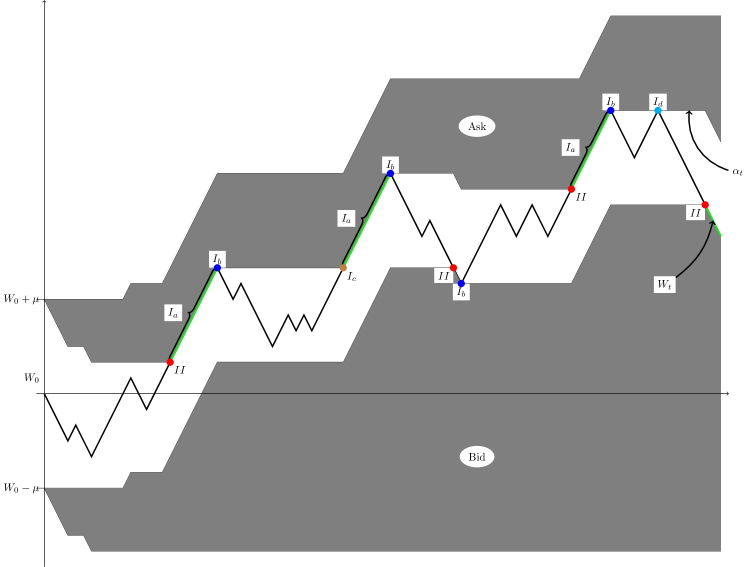
Figure 1: A schematic illustration of different types of trading times

We introduce an alternative representation for the best ask process $\alpha$. This will be used in the next sections for characterising the time to next trade in a probabilistic way. Denote by

$$w^{\ast}(s,t):=\sup\left\{w(r):r\in\left[s,t\right]\right\},\quad w_{\ast}(s,t):=\inf\left\{w(r):r\in\left[s,t\right]\right\}$$ (18)

the running maximum respectively minimum of the path $w$ in the interval $[s,t]$.

Definition 11.

Let

$$\Gamma_{s}:=\inf\{t\geq s:w(t)=w_{\ast}(s,t)+\mu\},\quad\Psi_{s}:=\inf\{t\geq s:w(t)=w^{\ast}(s,t)-\mu\}$$ (19)

and define for any $n\geq 0$ the times $\tau_{0}:=0$ and

$$\tau_{n+1}:=\begin{cases}\infty&\tau_{n}=\infty\\ \Gamma_{\tau_{n}}&n\text{ even, }t_{n}<\infty\\ \Psi_{\tau_{n}}&\text{otherwise.}\end{cases}$$ (20)

We start with a small observation for the time-points $\tau_{n}$, $n\in\mathbb{N}$.

Lemma 12.

The sequence $(\tau_{n})_{n\in\mathbb{N}}$ is strictly increasing until reaching $\infty$ and it has no finite accumulation point.

Proof.

Let $n\in\mathbb{N}$ such that $\tau_{n}\neq\infty$. By continuity of $w$ there is $\eta>0$ such that $|w(t)-w(\tau_{n})|<\mu/2$ for any $t\in[\tau_{n},\tau_{n}+\eta]$. Then, $w^{\ast}(\tau_{n},\tau_{n}+\eta)-w_{\ast}(\tau_{n},\tau_{n}+\eta)<\mu$ and hence $\Psi_{\tau_{n}},\Gamma_{\tau_{n}}>\tau_{n}+\eta$. Consequently, $\tau_{n+1}>\tau_{n}+\eta$.

Now assume by contradiction that $\tau_{n}\nearrow t$ for some $t\in(0,\infty)$. By continuity of $w$, there is $\eta>0$ such that $|w(t)-w(s)|<\mu/2$ for any $s\in[t-\eta,t]$. Moreover, there is $n\in\mathbb{N}$ such that $|\tau_{n}-t|\leq\eta$ and hence we have $t>\tau_{n+1}>\tau_{n}+\eta\geq t$. A contradiction.    

We can now identify the behavior of the best ask process $\alpha$ in terms of the times $(\tau_{n})_{n\geq 0}$.

Proposition 13.

We have

$$\alpha(t)=\begin{cases}w_{\ast}(\tau_{n},t)+\mu;&\tau_{n}\leq t<\tau_{n+1},~{}n\text{ {even}}\\ w^{\ast}(\tau_{n},t);&\tau_{n}\leq t<\tau_{n+1},~{}n\text{ {odd.}}\end{cases}$$

for any $t>0$. Moreover, $\alpha$ is a continuous function of finite variation which is non-increasing on $\{t:\exists n\in\mathbb{N}:\tau_{n}\leq t<\tau_{n+1},n\text{ even}\}$ and non-decreasing on the compliment.

Proof.

Define

$$\gamma(t):=\begin{cases}w_{\ast}(\tau_{n},t)+\mu;&\tau_{n}\leq t<\tau_{n+1},~{}n\text{ {even}}\\ w^{\ast}(\tau_{n},t);&\tau_{n}\leq t<\tau_{n+1},~{}n\text{ {odd.}}\end{cases}$$

for any $t>0$. We first show that $\gamma$ is continuous. Clearly, $\gamma$ is càdlàg and it is continuous outside $\{\tau_{n}:n\geq 0\}$ by definition. Let $n\geq 1$ with $\tau_{n}\neq\infty$.

Case 1: $n$ is even. By definition we have $\tau_{n}=\Psi_{\tau_{n-1}}$ and hence $w(\tau_{n})+\mu=w^{\ast}(\tau_{n-1},\tau_{n})$.

$$\gamma(\tau_{n}-) =\lim_{t\nearrow\tau_{n}}\gamma(t)=\lim_{t\nearrow\tau_{n}}w^{\ast}(\tau_{n-1},t)=w^{\ast}(\tau_{n-1},\tau_{n})$$

$$=w(\tau_{n})+\mu=w_{\ast}(\tau_{n},\tau_{n})+\mu=\gamma(\tau_{n}).$$

Case 2: $n$ is odd. This is proved analogously like the even case.

Thus $\gamma$ is a continuous function. Next we show that $\alpha=\gamma$. Now, let $t\in(\tau_{0},\tau_{1}]$. Then, $\gamma(t)=w_{*}(t_{0},t)+\mu$ and $\{w(s):s\in[0,t]\}=[w_{*}(0,t),w^{*}(0,t)]$. Hence $L_{t}^{u}>0$ for Lebesgue almost any $u\in[w_{*}(0,t),w^{*}(0,t)]$ and $L_{t}^{u}=0$ for any $u\in\mathbb{R}\backslash[w_{*}(0,t),w^{*}(0,t)]$. Consequently,

$$\alpha(t)=\inf\{x>w(t):V(t,x)>0\}=w_{*}(0,t)+\mu=\gamma(t).$$

Now let

$$I:=\{n\in\mathbb{N}:\forall t\in(\tau_{n},\tau_{n+1}]:\alpha(t)=\gamma(t)\}.$$

Let $n\in I\cup\{0\}$ and $t\in[\tau_{n+1},\tau_{n+2}]$.

Case 1: $n+1$ is even. Then, $\gamma(t)=w^{*}(\tau_{n+1},t)$ and $w(t)\leq w_{*}(\tau_{n+1},\tau_{n+2})+\mu$ by definition of $\gamma$ and $\tau_{n+2}$. Consequently,

$$w^{*}(\tau_{n+1},\tau_{n+2})=w_{*}(\tau_{1},\tau_{2})+\mu$$

and hence

$$V(t,x)=\left(V(\tau_{n+1},x)+L_{t}^{x-\mu}-L_{\tau_{n+1}}^{x-\mu}\right)\mathbf{1}_{\{w^{*}(\tau_{n+1},t)<x\}}\geq V(\tau_{n+1},x)\mathbf{1}_{\{w^{*}(\tau_{n+1},t)<x\}}.$$

Lemma 41 yields $\alpha(t)=w^{*}(\tau_{n+1},t)=\gamma(t)$.

Case 2: $n+1$ is odd. This works similar and we get $n+1\in I$.

By induction $\mathbb{N}=I\cup\{0\}$ which yields the claim.    

Corollary 14.

$\tau_{1}$ is the first (ask) trade and $\tau_{2n-1}$ denotes the $n$-th Type II trade (in the ask order book) for any $n\in\mathbb{N}$.

In view of this corollary we define, for mathematical convenience, the first trade to be of Type II.

Proof.

The first statement is immediate from the definition and the second statement follow immediately from Proposition 13.    

Remark 15.

In this section we have not used any specific properties of Brownian motion. In fact, we solely argued from the existence of a continuous occupation density which exists a.s. for many processes.

Let $X$ be any continuous semimartingale such that its quadratic variation is given by $[X,X](t)=\int_{0}^{t}c(X(s))ds$ where $c:\mathbb{R}\rightarrow(0,\infty)$ is a continuous function. [RY99, VI.1.7] yields that it has local time $L$ which is continuous in time and càdlàg in its space variable. [RY99, Corollary VI.1.6] yields that for any Borel set $A\in\mathcal{B}(\mathbb{R})$ we have

$$\int_{0}^{t}1_{\{X(s)\in A\}}ds=\int_{0}^{t}\frac{1_{\{X(s)\in A\}}}{c(X(s))}d[X,X](s)=\int_{A}\frac{L_{t}^{x}}{c(x)}dx$$

and, hence, $X$ has occupation density $\rho^{t}_{x}=\frac{L_{t}^{x}}{c(x)}$, $x\in\mathbb{R}$, $t\geq 0$. In particular, if its local time posses a continuous version, then so does its occupation density.

For more details on occupation densities see [GH80].

Remark 16.

Throughout this section we worked with the specific Dirac order placement. However, a close inspection of the arguments reveals that this is not strictly necessary to obtain the preceeding results. If orders are placed with respect to some measure $G$ instead, as in Equation (9), and $0\notin\mathrm{supp}(G)$, then defining $\mu:=\inf\mathrm{supp}(G|_{\mathcal{B}(\mathbb{R}_{+})})$ allows to obtain the same results as presented in this section as long as $\mu>0$.

4 Analysis of the Brownian order book with Dirac order placement

4.1 Characterizing trading times via a doubly reflected Brownian motion

We return to our stochastic setup as in Section 2.1. Our aim is now to characterize trading times via a doubly reflected Brownian motion. The results from the preceding section hold almost surely by the occupation times formula [RY99, Theorem VI.1.6] and [RY99, Theorem VI.1.7].

Remark 17.

Firstly, we observe that $(\tau_{n})_{n\geq 0}$ from Definition 11 is an increasing sequence of stopping times.

Up to here we have essentially gathered pathwise properties which do not rely on the specific structure of the Brownian motion except for the continuous sample path property and the existence of a continuous occupation density. This, however, holds for many other processes as well, cf. [Pro04, Theorem IV.76, Corollary IV.2]. For the rest of this section we consider features of trading times which appear to be more specific to the Brownian motion.

Definition 18.

Let $\mu>0$. A $[0,\mu]$-valued stochastic process $X$ is called a doubly reflected Brownian motion if

$$f(X(t))-\int_{0}^{t}\frac{1}{2}f^{\prime\prime}(X(s))ds,\quad t\geq 0$$

is a martingale for any twice continuously differentiable function $f:[0,\mu]\rightarrow\mathbb{R}$ with $f^{\prime}(0)=0=f^{\prime}(\mu)$.

Recall that [EK86, Theorems 8.1.1, 4.5.4] yield that such a process exist and [EK86, Theorem 4.4.1] yields that its process law is uniquely determined by its initial distribution $P^{X(0)}$.

Theorem 19.

The process $\alpha-W$ is a doubly reflected Brownian motion on the interval $[0,\mu]$ with $(\alpha-W)(0)=\mu$. Moreover, we have $\Theta=\{t:(\alpha-W)(t)=0\}$.

Clearly, $W-\beta$ is another doubly reflected Brownian motion on the interval $[0,\mu]$ and $\underline{\Theta}=\{t:(W-\beta)(t)=0\}$.

Proof.

Let $f:[0,\mu]\rightarrow\mathbb{R}$ be a twice continuously differentiable function with $f^{\prime}(0)=0=f^{\prime}(\mu)$ and define $R:=W-\alpha$. Let

$$I:=\Bigg{\{}n\in\mathbb{N}: \textstyle E\left[f(R(\tau_{n}+1))-\frac{1}{2}\int_{\tau_{n}}^{\tau_{n+1}}f^{\prime\prime}(R(s))ds\middle|\mathcal{F}_{\eta}\right]=f(R(\eta))-\int_{\tau_{n}}^{\eta}\frac{1}{2}f^{\prime\prime}(R(s))ds$$

$$\text{ for any stopping time }\eta\in[\tau_{n},\tau_{n+1}]\Bigg{\}}$$

Let $n\in\mathbb{N}$ be even and define $X(t):=W(t+\tau_{n})-W(\tau_{n})$ and $X_{\ast}(t):=\inf\{t\geq 0:X(t)\}$. Then $X$ is a Brownian motion which is independent of $\mathcal{F}_{\tau_{n}}$ and Proposition 13 yields that $R(\eta+\tau_{n})=R(\tau_{n})-X(\eta)+X_{\ast}(\eta)$ for any random time $\eta$ which is bounded by $\Delta\tau_{n}:=\tau_{n+1}-\tau_{n}$. Moreover, the law of $X_{\ast}-X$ coincides with the law of $-|B|$ for some Brownian motion $B$, which follows from a well-known result of Lévy, see for example [RY99, Thm.VI.2.3, p.240], and hence

$$f(R(\tau_{n})+(X_{\ast}-X)^{\Delta\tau_{n}}(t))+\int_{0}^{t\wedge\Delta\tau_{n}}\frac{1}{2}f^{\prime\prime}(R(\tau_{n})+(X_{\ast}-X)(s))ds,\quad t\geq 0$$

is a martingale. Hence, $n\in I$. For odd $n\in\mathbb{N}$ similar arguments show that $n\in I$ and thus $I=\mathbb{N}$. The tower property yields that $(R(t)-\int_{0}^{t}\frac{1}{2}f^{\prime\prime}(R(s))ds)_{t\geq 0}$ is a martingale and hence $R$ is an $[0,\mu]$-valued process with $[R](t)=[W](t)=t$ and reflecting boundaries and hence a doubly reflected Brownian motion, cf. [EK86, p. 366].    

Next we show that there are no isolated trades, i.e. there are no trades of Type Id or Type IId.

Corollary 20.

We have no isolated trades, i.e., $P(\Theta_{\mathrm{I}_{d}}\cup\Theta_{\mathrm{II}_{d}}=\emptyset)=1$. In particular, we have

$$P(\Theta_{\mathrm{II}}=\Theta_{\mathrm{II}_{c}}) =1.$$

Proof.

By Theorem 19 we have to show that a doubly reflected Brownian motion on $[0,\mu]$ has $P$-a.s. no isolated zeros. Using the construction in [KS91], Section 2.8.C, we see that this is equivalent to show that a standard Brownian motion has $P$-a.s. no isolated times in the set $\{2z\mu:z\in\mathbb{Z}\}$. This is a consequence of [KS91], Theorem 9.6, Chapter 2.    

4.2 Stopping times and trading times

So far we have defined trading times pathwise: $t\in\mathbb{R}^{+}$ is a trading time for $w\in\mathbf{W}$ if $w(t)=\alpha(t,w)$. We say a random time $\tau$ is a trading time, if $W_{\tau}=\alpha(\tau)$ a.s. Next, we will give some examples of trading times which are also stopping times and we will show that a stopping time which is a trading time is not of Type Ib.

Lemma 21.

Let $\tau$ be a stopping time such that $P(\tau\in\Theta)=1$. Then $\Xi(\tau)=\tau$ $P$-a.s. In particular, $P(\tau\in\Theta_{\mathrm{I}_{b}})=0$.

Proof.

Let $\epsilon>0$ and define $B(t):=W(t+\tau)-W(\tau)$, $t\geq 0$. Then, $B$ is a standard Brownian motion. Let $\sigma_{\epsilon}$ be the time where $B$ attains its maximum on $[0,\epsilon]$. Then, $\sigma_{\epsilon}$ is measurable and $B(\sigma_{\epsilon})>0$ $P$-a.s. Hence $\tau+\sigma_{\epsilon}$ is a trading time and, consequently, $P(\Xi(\tau)=\tau)=1$.    

Corollary 14 together with Remark 17 reveals that the Type II trades can be enumerated by stopping times. Lemma 21 shows that the Type Ib trades are not stopping times. This leaves the question whether stopping times can be of Type Ia or Type Ic, which is, indeed, the case.

First entry times of high levels are actually Type Ia trades.

Example 22.

Let $x>\mu$ and $\gamma_{x}:=\inf\{t\geq 0:w(t)=x\}$. Then we have

$$P(\gamma_{x}\text{ is a Type~{}{Ia} trade})=1.$$

Proof.

By Proposition 13 we have $\alpha(t)\leq w^{*}(0,t)$ and clearly $w(t)\leq\alpha(t)$ for any $t\in[\tau_{1},\infty)$. Since

$$\tau_{1}=\inf\{t>0:w(t)=w^{*}(0,t)-\mu\}$$

we have $w^{*}(0,\tau_{1})\leq\mu$. Hence, we have $\tau_{1}\leq\gamma_{x}$. Thus we get

$$w^{*}(0,\gamma_{x})=x=w(\gamma_{x})\leq\alpha(\gamma_{x})\leq w^{*}(0,\alpha_{x}).$$

and hence $\gamma_{x}\in\Theta$.

Let $\epsilon\in(0,\gamma_{x})$. Then, there is $s_{\epsilon}\in(\gamma_{x}-\epsilon,\gamma_{x})$ such that $w(s_{\epsilon})=w^{*}(0,s_{\epsilon})>\mu$. Hence, $\alpha(s_{\epsilon})=w(s_{\epsilon})$ and we have $s_{\epsilon}\in\Theta$. This implies that $\Upsilon(\gamma_{x})=\gamma_{x}$. Lemma 21 yields that $\Xi(\gamma_{x})=\gamma_{x}$ $P$-a.s. Hence, $\gamma_{x}\in\Theta_{\mathrm{I}_{a}}$ $P$-a.s.    

Example 23.

There is a stopping time $\eta$ such that

$$P(\eta\text{ is a Type~{}{Ic} trade})=1.$$

Proof.

For a stopping time $\eta$ define the new stopping times

$$\gamma_{0}(\eta) :=\inf\{t\geq\eta:(\alpha-W)(t)=0\},$$

$$\gamma_{1}(\eta) :=\inf\{t\geq\eta:(\alpha-W)(t)=\mu/2\},$$

$$\gamma_{2}(\eta) :=\inf\{t\geq\eta:(\alpha-W)(t)\in\{0,\mu\}\}.$$

Clearly, $\gamma_{j}(\eta)$ is $P$-a.s. finite for any finite stopping time $\eta$, $j=0,1,2$. Moreover,

$$P((\alpha-W)(\gamma_{2}(\gamma_{1}(\eta)))=0)=1/2$$

by symmetry and the Markov property for any stopping time $\eta$. We have

$$A(\eta):=\{\gamma_{2}(\gamma_{1}(\gamma_{0}(\eta))):(\alpha-W)(\gamma_{2}(\gamma_{1}(\gamma_{0}(\eta))))=0\}\subseteq\Theta_{\mathrm{I}_{c}}$$

for any finite stopping time $\eta$.

Define $\eta_{0}:=\tau_{2}$ where $\tau_{2}$ is given in Definition 11. Observe that $w(\tau_{2})\neq\alpha(\tau_{2})$. Define recursively

$$\eta_{n+1}:=\begin{cases}\eta_{n}&\text{if $\alpha(\eta_{n})=w(\eta_{n})$},\\ \gamma_{2}(\gamma_{1}(\gamma_{0}(\eta_{n})))&\text{otherwise.}\end{cases}$$

Then, $(\eta_{n})_{n\in\mathbb{N}}$ converges $P$-a.s. in finitely many steps. Denote $\eta_{\infty}:=\lim_{n\rightarrow\infty}\eta_{n}$. Clearly, $\alpha(\eta_{\infty})=w(\eta_{\infty})$ $P$-a.s. Moreover, denote $\eta_{-}:=\eta_{\{\sup\{n\in\mathbb{N}:\eta_{n}\neq\eta_{\infty}\}\}}$. Then, we have $\gamma_{2}(\gamma_{1}(\gamma_{0}(\eta_{-})))=\eta_{\infty}$. Consequently,

$$P(\eta_{\infty}\in\Theta_{\mathrm{II}_{c}})=1.$$

   

5 Trading excursions

5.1 The trading excursion process

Theorem 19 shows that trading times correspond to the zeroes of the Markov processes $X$ and $Y$ defined by

$$X=\alpha-W,\quad Y=W-\beta.$$ (21)

This allows to study trading times by using excursion theory. Let us recapitulate briefly the terminology and notation of excursion theory, for background and more details we refer the reader to [RY99, Ch.XII] and [Blu92].

For $w\in\mathbf{W}$ define

$$R(w)=\inf\{t>0:w(t)=0\}.$$ (22)

Let $U^{+}$ denote all nonnegative functions $w$ such that $0<R(w)<\infty$, let $\delta$ denote the function that is identically zero, and set $U^{+}_{\delta}=U^{+}\cup\{\delta\}$, and let $\mathcal{U}^{+}_{\delta}$ denote the trace of the Borel $\sigma$-field on $\mathbf{W}$ in $U^{+}_{\delta}$.

First we note that $X$ is a continuous semi-martingale, namely doubly reflected Brownian motion on $[0,\mu]$. Thus it admits a local time at zero that satifies the Tanaka formula,

$$L_{t}(X)=|X_{t}|-|X_{0}|-\int_{0}^{t}\operatorname{sgn}(X_{s})dX_{s},\quad t\geq 0.$$ (23)

Consider the inverse local time process,

$$\tau_{s}(X)=\inf\{t\geq 0:L_{t}(X)\geq s\},\quad s>0.$$ (24)

Definition 24.

The trading excursion process for the ask-side is the process $(\overline{e}_{s},s>0)$, i.e. the zero-excursion process for $X$. The trading excursion process for the bid-side is the process $(\underline{e}_{s},s>0)$ i.e. the zero-excursion process for $Y$.

This means, that $\overline{e}$ and $\underline{e}$ are defined on $\Omega\times\mathbb{R}_{+}$ and take values in $U_{\delta}^{+}$ as follows, see [RY99, Def.XII.2.1, p.480]:

1. If $\Delta\tau_{s}(X)>0$, then $\overline{e}_{s}(w)$ is the map

   $$r\mapsto\overline{e}_{s}(r,w)=I_{[r\leq\Delta\tau_{s}(w)]}X_{\tau_{s-}(w)+r}(w),$$ (25)

2. if $\Delta\tau_{s}(X)=0$, then $\overline{e}_{s}(w)=\delta.$

Thus $\overline{e}$ and $\underline{e}$ take values in the function space $U_{\delta}^{+}$. Illustrations for the trading excursion process are given in Figures 2,3,4 for a Type I trade resp. in Figures 5,6,7 for a Type II trade.

Theorem 25.

The bid and ask trading excursion processes are Poisson point processes.

Proof.

The previous proposition says that ask trading excursions for $W$ correspond to excursions from zero for $\alpha-W$. The process $\alpha-W$ is a doubly reflected Brownian motion, which is a Markov process. We can apply [Blu92, Thm.3.18, p.95]. The same argument holds for $W-\beta$.    

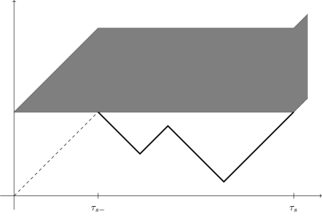
Figure 2: Ask trade of Type I

Figure 3: Corresponding path of $\alpha-W$

Figure 4: Corresponding excursion $\overline{e}_{s}$

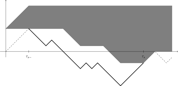
Figure 5: Ask trade of Type II

Figure 6: Corresponding path of $\alpha-W$

Figure 7: Corresponding excursion $\overline{e}_{s}$

5.2 Description of the trading excursion measure

For any Poisson point process there exists an intensity measure.

Definition 26.

Let us denote the intensity measures for the bid and ask excursion processes by $\underline{n}$ and $\overline{n}$.

The measures $\underline{n}$ and $\overline{n}$ are $\sigma$-finite measures on $\mathcal{U}_{\delta}^{+}$, and satisfy

$$\underline{n}(\Gamma)=\frac{1}{t}E[\underline{N}_{t}^{\Gamma}],\quad\overline{n}(\Gamma)=\frac{1}{t}E[\overline{N}_{t}^{\Gamma}],\quad t>0,$$ (26)

where

$$\underline{N}_{t}^{\Gamma}=\sum_{0<s<t}I_{\Gamma}(\underline{e}_{s}),\quad\overline{N}_{t}^{\Gamma}=\sum_{0<s<t}I_{\Gamma}(\overline{e}_{s}),\quad\Gamma\in\mathcal{U}_{\delta}^{+}.$$ (27)

Remark 27.

In the following we focus on $\underline{n}$ because $\overline{n}=\underline{n}$.

Let us recall a convenient notation from Williams [Wil91, Sec.5.0, p.49], for the integral of a measurable function $F:U_{\delta}^{+}:\to\mathbb{R}$ with respect to the measure $\underline{n}$ and a set $\Gamma\in\mathcal{U}_{\delta}^{+}$,

$$\underline{n}(F)=\int F(u)\underline{n}(du),\quad\underline{n}(F;\Gamma)=\int_{\Gamma}F(u)\underline{n}(du).$$ (28)

For better readability, we shall also write $\underline{n}[F]$ and $\underline{n}[F;\Gamma]$ instead of $\underline{n}(F)$ and $\underline{n}(F;\Gamma)$ when the expressions for $F$ or $\Gamma$ are more involved. Furthermore, let us introduce for $x>0$ and $u\in C(\mathbb{R}_{+};\mathbb{R})$ the hitting time

$$T_{x}(u)=\inf\{t>0:u(t)=x\}.$$ (29)

We can now give a description of the trading excursion measure that is inspired by Williams’ description of the Ito measure. Pick three independent processes, namely two $\operatorname{BES}^{3}(0)$ processes $\rho$ and $\tilde{\rho}$, and a standard Brownian motion $b$ (a $\operatorname{BES}^{3}(0)$ processes is a process whose law coincides with the law of $|B|$ where $B$ is a three dimensional standard Brownian motion starting in zero.). For all $x\in(0,\mu)$ we define a process $Z^{x}$ by

$$Z^{x}=\left\{\begin{array}[]{ll}\rho_{t}&0\leq t\leq T_{x}(\rho),\\ x-\tilde{\rho}_{t-T_{x}(\rho)}&T_{x}(\rho)<t\leq T_{x}(\rho)+T_{x}(\tilde{\rho}),\\ 0&t>T_{x}(\rho)+T_{x}(\tilde{\rho}),\end{array}\right.$$ (30)

and we define

$$Z^{\mu}=\left\{\begin{array}[]{ll}\rho_{t}&0\leq t\leq T_{\mu}(\rho),\\ \mu-|b_{t-T_{\mu}(\rho)}|&T_{\mu}(\rho)<t\leq T_{\mu}(\rho)+T_{\mu}(|b|),\\ 0&t>T_{\mu}(\rho)+T_{\mu}(|b|).\end{array}\right.$$ (31)

Let us introduce length $R$ and height $H$ for excursions $u\in U_{\delta}^{+}$ by

$$R(u)=\inf\{t>0:u(t)=0\},\quad H(u)=\sup\{u(t):0\leq t\leq R(u)\},$$ (32)

and

$$R_{I}(u)=R(u)I_{H(u)<\mu},\quad R_{II}(u)=R(u)I_{H(u)\geq\mu}.$$ (33)

So, $R_{I}(u)$ is the length of a trading excursion that ends with a Type Ic trade, and zero otherwise, whereas $R_{II}(u)$ is the length of a trading excursion that ends with a Type II trade, and zero otherwise.

Theorem 28.

For any $\Gamma\in\mathcal{U}_{\delta}^{+}$

$$\underline{n}(\Gamma)=\frac{1}{2}\int_{0}^{\mu}P[Z^{x}\in\Gamma]x^{-2}dx+\frac{1}{2\mu}P[Z^{\mu}\in\Gamma].$$ (34)

Proof.

This is a combination of two results about Williams’ description of the Ito measure, namely the excursion conditioned on a fixed height, see [RY99, Thm.XII.4.5, p.499], and the decomposition of the excursion straddling the first hitting time of level $\mu$ as presented in [Rog81, Prop.3.3, p.237] and [YY13, 6.8 (a), p.75].    

Corollary 29.

Let $F:C(\mathbb{R}_{+};\mathbb{R})\to\mathbb{R}$ be a non-negative measurable function. Then

$$\underline{n}(F)=\frac{1}{2}\int_{0}^{\mu}E[F(Z^{x})]x^{-2}dx+\frac{1}{2\mu}E[F(Z^{\mu})].$$ (35)

The formula holds also true if $F$ is real- or complex-valued and $\underline{n}(|F|)<\infty$, or equivalently, if

$$\int_{0}^{\mu}E[|F(Z^{x})|]x^{-2}dx+E[|F(Z^{\mu})|]<\infty.$$ (36)

Corollary 30.

We have

$$\underline{n}[H\geq x]=\left\{\begin{array}[]{ll}\displaystyle\frac{1}{2x}&0<x\leq\mu,\\ &\\ \displaystyle 0&x>\mu,\end{array}\right.$$ (37)

and

$$\underline{n}[H\in dx]=\frac{1}{2x^{2}}I_{(0,\mu)}(x)dx+\frac{1}{2\mu}\delta_{\mu}(dx).$$ (38)

6 The hyperbolic function table for intertrading times

6.1 The hyperbolic table under the trading excursion measure

A trading excursion starts with a Ib trade. In this section we study the time to the next trade after a trading excursion. Consider the time interval from a Ib ask trade to the next trade. This is a trading excursion interval for $W$, and by Theorem 19, a zero excursion interval for $\alpha-W$. So the time to the next trade is just the length of an excursion interval. We shall start with the trading excursion space $(U_{\delta}^{+},\mathcal{U}_{\delta}^{+},\underline{n})$ and then transfer the results to the probability space $(\Omega,\mathcal{F},P)$.

The time to the next trade for a trading excursion $u\in U_{\delta}^{+}$ is the length $R$ of the trading excursion, the type of the next trade depends on the height $H$. If $H(u)<\mu$ the next trade is of Type I, if $H(u)\geq\mu$ it is of Type II. Below we shall see that $\underline{n}[H>\mu]=0$.

We state the following theorems for real $\lambda>0$. Using arguments based on results on the analyticity of Laplace transforms it can be shown that they extend to a larger complex domain.

Lemma 31 (On the joint law of $R$ and $H$ under $\underline{n}$).

Suppose $\lambda>0$ and $0<y\leq\mu$, then we have

$$\underline{n}[1-e^{-\lambda R};H<y]=-\frac{1}{2y}+\frac{1}{2}\sqrt{2\lambda}\coth(y\sqrt{2\lambda}).$$ (39)

Proof.

For this proof we use the description of the trading excursion measure given in Section 5.2. From (30) we note first that $R(Z^{x})=T_{x}(\rho)+T_{x}(\tilde{\rho})$ and $H(Z^{x})=x$ for $0<x<\mu$. The random variables $T_{x}(\rho)$ and $T_{x}(\tilde{\rho})$ are independent first hitting times of $\operatorname{BES}^{3}$-processes for level $x$. The corresponding Laplace transform is well-known, namely

$$E[e^{-\lambda T_{x}(\rho)}]=E[e^{-\lambda T_{x}(\tilde{\rho})}]=\frac{x\sqrt{2\lambda}}{\sinh(x\sqrt{2\lambda})}.$$ (40)

See [Ken78, (3.8), p.762] with $\nu=1/2$, see also [BPY01, Tab.2, Row 3, Col.1, p.450 and Sec.4.5, p.453]. From Corollary 29 we get

$$\underline{n}[1-e^{-\lambda T};H<y]=\frac{1}{2}\int_{0}^{\mu}E[1-e^{-\lambda R(Z^{x})};H(Z^{x})<y]x^{-2}dx$$ (41)

$$\qquad=\frac{1}{2}\int_{0}^{y}E[1-e^{-\lambda R(Z^{x})}]x^{-2}dx=\frac{1}{2}\int_{0}^{y}\left(1-E\left[e^{-\lambda(T_{x}(\rho)+T_{x}(\tilde{\rho}))}\right]\right)x^{-2}dx$$ (42)

$$\qquad=\frac{1}{2}\int_{0}^{y}\left[1-\left(\frac{x\sqrt{2\lambda}}{\sinh(x\sqrt{2\lambda})}\right)^{2}\right]x^{-2}dx=-\frac{1}{2y}+\frac{1}{2}\sqrt{2\lambda}\coth(y\sqrt{2\lambda}).$$ (43)

   

Theorem 32 (Hyperbolic table under the trading excursion measure).

Let $\lambda>0$.

1. We have for the length $R_{I}$ of the trading excursion to the next Type $I$ trade

   $$\underline{n}[1-e^{-\lambda R_{I}}]=-\frac{1}{2\mu}+\frac{1}{2}\sqrt{2\lambda}\coth(\mu\sqrt{2\lambda}),$$ (44)

2. for the length $R_{II}$ of the trading excursion to the next Type $II$ trade

   $$\underline{n}[1-e^{-\lambda R_{II}}]=\frac{1}{2\mu}-\sqrt{2\lambda}\operatorname{csch}(2\mu\sqrt{2\lambda}),$$ (45)

3. and for the length $R$ of the trading excursion to the next trade

   $$\underline{n}[1-e^{-\lambda R}]=\frac{1}{2}\sqrt{2\lambda}\tanh(\mu\sqrt{2\lambda}).$$ (46)

Proof.

Part (1) is due to [YY13, p.66] and agrees with the result from Theorem 31 for the special case $y=\mu$.

For Part (2) we note first from (31) that $R(Z^{\mu})=T_{\mu}(\rho)+T_{\mu}(|b|)$, with $\rho$ a $\operatorname{BES}^{3}$-process and $|b|$ an independent reflected Brownian motion, The random variables $T_{\mu}(\rho)$ and $T_{\mu}(|b|)$ are their first hitting times of level $\mu$ respectively, and $H(Z^{\mu})=\mu$. The corresponding Laplace transforms are well-known, namely

$$E[e^{-\lambda T_{\mu}(\rho)}]=\mu\sqrt{2\lambda}\operatorname{csch}(\mu\sqrt{2\lambda}),\quad E[e^{-\lambda T_{\mu}(|b|)}]=\frac{1}{\cosh(\mu\sqrt{2\lambda})}.$$ (47)

See [Ken78, (3.8), p.762] with $\nu=1/2$ and $\nu=-1/2$, see also [BPY01, Tab.2, Row 3, Col.3, p.450 and Sec.4.5, p.453]. Thus we get by Corollary 29

$$\underline{n}[e^{-\lambda R_{II}};H=\mu] = \frac{1}{2\mu}E[e^{-\lambda(T_{\mu}(\rho)+T_{\mu}(|b|))}]$$ (48)

$$= \frac{\sqrt{2\lambda}}{2\sinh(\mu\sqrt{2\lambda})}\frac{1}{\cosh(\mu\sqrt{2\lambda})}=\sqrt{2\lambda}\operatorname{csch}(2\mu\sqrt{2\lambda}).$$ (49)

Part (3) is obtained by adding Parts (1) and (2) and an elementary duplication formula for hyperbolic functions, [AS64, 4.5.31, p.84].    

Remark 33.

We can rewrite (44) and (45) as follows:

$$\underline{n}[1-e^{-\lambda R}I_{H<\mu}]=\frac{1}{2}\sqrt{2\lambda}\coth(\mu\sqrt{2\lambda}),$$ (50)

and

$$\underline{n}[e^{-\lambda R}I_{H=\mu}]=\sqrt{2\lambda}\operatorname{csch}(2\mu\sqrt{2\lambda}).$$ (51)

Note that $\underline{n}[e^{-\lambda R}I_{H<\mu}]=\infty$ for all $\lambda>0$ though.

We can describe the distributions of $R$ and $H$ under $\underline{n}$ more explicitly using theta functions. There are many notations and parametrizations for theta functions, see [WW96, Sec.21.9, p.487] for an overview. We choose a variant inspired by [Dev09], which allows a simple statement of transformation formulas. Let

$$\theta_{2}(x) = 2\sum_{n\geq 1}e^{-(n-1/2)^{2}\pi x},$$ (52)

$$\theta_{3}(x) = 1+2\sum_{n\geq 1}e^{-n^{2}\pi x},$$ (53)

$$\theta_{4}(x) = 1+2\sum_{n\geq 1}(-1)^{n}e^{-n^{2}\pi x}.$$ (54)

Theorem 34 (Theta table).

We have

1. $$\underline{n}[R>x,H<y]=\frac{1}{2y}\left[\theta_{3}\left(\frac{\pi x}{2y^{2}}\right)-1\right],\quad x>0,0<y\leq\mu$$ (55)

2. $$\underline{n}[R>x,H=\mu]=\frac{1}{2\mu}\left[1-\theta_{4}\left(\frac{\pi x}{8\mu^{2}}\right)\right],\quad x>0,$$ (56)

3. $$\underline{n}[R>x]=\frac{1}{2\mu}\theta_{2}\left(\frac{\pi x}{2\mu^{2}}\right),\quad x>0.$$ (57)

Proof.

By Fubini’s Theorem and (39) we compute the Laplace transform

$$\int_{0}^{\infty}e^{-\lambda x}\underline{n}[R>x,H<y]dx = \frac{1}{\lambda}\underline{n}[1-e^{-\lambda R};H<y]$$ (58)

$$= -\frac{1}{2\lambda y}+\frac{1}{\sqrt{2\lambda}}\coth(y\sqrt{2\lambda}).$$ (59)

This agrees with the Laplace transform of (55), which is known resp. easily checked by termwise-transformation followed by an application of the partial fraction expansion of the hyperbolic cotangent. Equations (56) and (57) can be proved in a similar way.    

For later usage we differentiate those formulas with respect to $x$ and $y$ and obtain

$$\underline{n}[R\in dx]=-\frac{\pi}{4\mu^{3}}\theta_{2}^{\prime}\left(\frac{\pi x}{2\mu^{2}}\right)dx.$$ (60)

$$\underline{n}[R\in dx,H\in dy] = \left[\frac{3\pi}{4y^{4}}\theta_{3}^{\prime}\left(\frac{\pi x}{2y^{2}}\right)+\frac{\pi^{2}x}{4y^{6}}\theta_{3}^{\prime\prime}\left(\frac{\pi x}{2y^{2}}\right)\right]I_{(0,\mu)}(y)dxdy$$ (62)

$$\qquad\qquad-\frac{\pi}{16\mu^{3}}\theta_{4}^{\prime}\left(\frac{\pi x}{8\mu^{2}}\right)dx\delta_{\mu}(dy).$$

6.2 The hyperbolic table under the probability measure

We have two general devices for Poisson point processes to relate results for the probability measure to results about its intensity measure, namely the Exponential Formula [RY99, Prop.XII.1.12, p.476] and the Master Formula [RY99, Prop.XII.1.10 and Corl.XII.1.11, p.475].

Theorem 35 (Hyperbolic table in exponential form).

Let $\lambda>0$ and $t>0$.

1. We have for the length $R_{I}$ of the trading excursion to the next Type $I$ trade

   $$E\left[\exp\left\{-\lambda\sum_{0<s\leq t}R_{I}(\underline{e}_{s})\right\}\right]=\exp\left[-t\left(-\frac{1}{2\mu}+\frac{1}{2}\sqrt{2\lambda}\coth(\mu\sqrt{2\lambda})\right)\right],$$ (63)

2. for the length $R_{II}$ of the trading excursion to the next Type $II$ trade

   $$E\left[\exp\left\{-\lambda\sum_{0<s\leq t}R_{II}(\underline{e}_{s})\right\}\right]=\exp\left[-t\left(\frac{1}{2\mu}-\sqrt{2\lambda}\operatorname{csch}(2\mu\sqrt{2\lambda})\right)\right],$$ (64)

3. and for the length $R$ of the trading excursion to the next trade

   $$E\left[\exp\left\{-\lambda\sum_{0<s\leq t}R(\underline{e}_{s})\right\}\right]=\exp\left[-t\left(\frac{1}{2}\sqrt{2\lambda}\tanh(\mu\sqrt{2\lambda})\right)\right].$$ (65)

Proof.

This follows from the exponential formula with $f(s,u)=\lambda R_{I}(u)$, $f(s,u)=\lambda R_{II}(u)$, $f(s,u)=\lambda R(u)$ and Theorem 32 above.    

Remark 36.

The sums on the left hand sides are summing over excursions until the local time reaches the level $t$, which corresponds to real time $\tau_{t}$.

Corollary 37 (Hyperbolic table in additive form).

Suppose $\lambda>0$ and $t>0$.

1. We have for the length $R_{I}$ of the trading excursion to the next Type $I$ trade

   $$E\left[\sum_{0<s\leq t}\left(1-e^{-\lambda R_{I}(\underline{e}_{s})}\right)\right]=t\left[-\frac{1}{2\mu}+\frac{1}{2}\sqrt{2\lambda}\coth(\mu\sqrt{2\lambda})\right].$$ (66)

2. We have for the time to the next trade $T$ assuming it is Type II

   $$E\left[\sum_{0<s\leq t}\left(1-e^{-\lambda R_{II}(\underline{e}_{s})}\right)\right]=t\left[\frac{1}{2\mu}-\sqrt{2\lambda}\operatorname{csch}(2\mu\sqrt{2\lambda})\right].$$ (67)

3. We have for the time to the next trade $T$

   $$E\left[\sum_{0<s\leq t}\left(1-e^{-\lambda R(\underline{e}_{s})}\right)\right]=t\left[\frac{1}{2}\sqrt{2\lambda}\tanh(\mu\sqrt{2\lambda})\right].$$ (68)

Proof.

This follows from the master formula [RY99, XII.1.10] with $f(s,u)=1-e^{-\lambda R_{I}(u)}$, $f(s,u)=1-e^{-\lambda R_{II}(u)}$, $f(s,u)=1-e^{-\lambda R(u)}$ respectively and Theorem 32 above.    

7 Laplace transform for the avalanche length

Orders in the LOB get executed via avalanches. In other words, limit orders may accumulate on some levels, and when the price process crosses those values, we will see a sudden decrease of the number of orders. We take record if there is no order execution in a time period lasting longer than $\varepsilon>0$.

Recall from Definitions 4 and 6 that $\Theta$ denotes the set of all trading times, $\Upsilon(t)$ (resp. $\Xi$) denotes the time of last trade before (resp. next trade after) time $t$.

Definition 38.

Let

$$a\in\Theta,~{}\Upsilon(a)\leq(a-\varepsilon)_{+},~{}b\in\Theta,~{}\Xi(b)\geq b+\varepsilon,$$ (69)

$$\Xi(t)\leq t+\varepsilon\quad\forall t\in(a,b).$$ (70)

An $\varepsilon$-avalanche is defined as the process $\left\{W_{t}:a\leq t\leq b\right\}$. We call $a$ and $b$ start and end of the avalanche. The corresponding $\varepsilon$-avalanche length is $b-a$.

There is a sequence of stopping times $(T_{n}^{a})_{n\geq 1}$ enumerating the start of avalanches, and a sequence of honest times $(T_{n}^{e})_{n\geq 1}$ enumerating the end of avalanches (for the completed filtration). We are interested into the distribution of the avalanche length for which we will rely on the hyperbolic table of the distribution of intertrading times.

Theorem 39.

Let $T$ be a stopping time starting an $\varepsilon$-avalanche and $A^{\varepsilon}$ be the corresponding avalanche length. Then we have the Laplace transform

$$E\left[e^{-\lambda A^{\varepsilon}}\right]=\frac{H(\varepsilon)}{H(\varepsilon)+\int_{0}^{\varepsilon}(1-e^{-\lambda x})h(x)dx}.$$ (71)

where

$$H(\varepsilon)=\frac{1}{2\mu}\theta_{2}\left(\frac{\pi\varepsilon}{2\mu^{2}}\right),\quad h(x)=-\frac{\pi}{4\mu^{3}}\theta_{2}^{\prime}\left(\frac{\pi x}{2\mu^{2}}\right).$$ (72)

Proof.

Let $\underline{e}$ denote the trading excursion process for the ask side. We have seen that it is a Poisson point process with intensity measure $\underline{n}$. Let $R$ denote the excursion length functional. Set

$$X_{s}=\sum_{0\leq r\leq s}R(e_{r}),\quad s\geq 0.$$ (73)

By Theorem 35 and Theorem 34 we see that $X$ is a Lévy process with Lévy measure

$$\nu_{X}(dx)=\underline{n}(dx)=h(x)dx,\quad x>0.$$ (74)

For $\varepsilon>0$ we can write $X=J+Y$ with

$$Y_{s}=\sum_{0\leq r\leq s}\Delta X_{s}I_{\Delta X_{s}>\varepsilon},\quad J_{s}=X_{s}-Y_{s},\quad s\geq 0.$$ (75)

Then $J$ and $Y$ are two independent Lévy processes with Lévy measures

$$\nu_{J}(dx)=I_{x\leq\varepsilon}h(x)dx,\quad\nu_{Y}(dx)=I_{x>\varepsilon}h(x)dx,\quad x>0.$$ (76)

Let $S=\inf\{s\geq 0:\Delta Y_{s}>0\}$. This is the first jump time of a compound Poisson process with Lévy measure $\nu_{Y}$ and thus exponential with parameter $\beta$ given by

$$\beta=\nu_{Y}(\mathbb{R}_{+})=\underline{n}[R>\epsilon]=H(\epsilon).$$ (77)

The Lévy-Khintchine formula for the cumulant of $J$ says

$$\kappa(\lambda)=\int_{0}^{\infty}(e^{-\lambda x}-1)\nu_{J}(dx).$$ (78)

A straight integration gives

$$\kappa(\lambda)=-\int_{0}^{\varepsilon}(1-e^{-\lambda x})h(x)dx.$$ (79)

The full avalanche length is $A=J_{S}$. By independence we obtain the Laplace transform

$$E[e^{-\lambda A}]=\int_{0}^{\infty}e^{\kappa(\lambda)s}\beta e^{-\beta s}ds=\frac{\beta}{\beta-\kappa(\lambda)}$$ (80)

and combining this with the results above yields the result.    

Remark 40.

Let us ignore Type II trades, and assume that orders are only executed as in the Type I case. Dassios and Wu [DW15] derive the Laplace transform of the avalanche length $L^{\varepsilon}$ in the context of Parisian options. The same formula can be inferred (Dudok de Wit [DdW13]) from the Lévy measure of the subordinator consisting of Brownian passage times. It results that

$$E\left[e^{-\lambda L^{\varepsilon}}\right]=\frac{1}{\sqrt{\lambda\varepsilon\pi}\mathrm{\mathop{\mathrm{e}rf}}\left(\sqrt{\lambda\varepsilon}\right)+e^{-\lambda\varepsilon}},$$ (81)

which can be proven in a completely analogous way by choosing $\tilde{h}\left(x\right)=x^{-3/2}/\sqrt{2\pi}$, which is the density of the excursion length $T$ under the Ito measure $n$, instead of function $h$. In this case the integral in the denominator can be evaluated in terms of the error function by some elementary computations.

8 Technical remarks, discussions and proofs

8.1 Depth of the order book after the first trade

The next lemma states that the limit order book has an order depth of at least $\mu$ after the first trade $\tau_{1}$ has happened. Here, we work under the same assumptions as in Section 3.

Lemma 41.

$\tau_{1}$ is the first trade and for any $t\geq\tau_{1}$ there is a closed set $K_{t}$ which is a Lebesgue null-set such that

$$(\alpha(t),\alpha(t)+\mu)\backslash K_{t}\subseteq\{x\in\mathbb{R}:V(t,x)>0\}\subseteq(\alpha(t),\infty).$$

Proof.

The last inclusion is trivial.

For $t\in[0,\tau_{1}]$ we have $V(t,x)=0$ for any $x<w_{\ast}(0,\tau_{1})+\mu$ and, hence, the first trade does not take place in $[0,\tau_{1})$. Moreover, we have

$$\{w(t):t\in[0,\tau_{1}]\}=[w_{\ast}(0,\tau_{1}),w^{*}(0,\tau_{1})]=[w_{\ast}(0,\tau_{1}),w_{\ast}(0,\tau_{1})+\mu].$$

Consequently, $L_{\tau_{1}}^{\cdot}$ has support $[w_{\ast}(0,\tau_{1}),w_{\ast}(0,\tau_{1})+\mu]$. Let

$$K_{\tau_{1}}:=\{x\in[w_{\ast}(0,\tau_{1}),w_{\ast}(0,\tau_{1})+\mu]:L_{\tau_{1}}^{x}=0\}=\{x\in[w^{\ast}(0,\tau_{1}),w^{\ast}(0,\tau_{1})+\mu]:L_{\tau_{1}}^{x-\mu}=0\}.$$

Then, $K_{\tau_{1}}$ is closed by continuity of the occupation density and it is a Lebesgue null-set. Clearly, we have

$$\{x:V(\tau_{1},x)>0\}=\{x:L_{\tau_{1}}^{x-\mu}>0\}=[w^{\ast}(0,\tau_{1}),w^{\ast}(0,\tau_{1})+\mu]\backslash K_{\tau_{1}}.$$

The first claim follows.

Let $T\in[\tau_{1},\infty]$ be maximal such that for any $t\in[\tau_{1},T)$ the claim holds. Assume by contradiction that $T<\infty$. By continuity of $w$ the claim holds at time $T$. Again by continuity there is $\delta>0$ such that $w^{\ast}(T,T+\delta)<w_{\ast}(T,T+\delta)$. We have

$$V(t,x)=V(T,x)\mathbf{1}_{\sigma_{T,t}(x)=T}+L^{x-\mu}_{t}-L^{x-\mu}_{\sigma_{T,t}(x)}$$

where $\sigma_{T,t}(x):=\inf\{s\in[T,t]:w(s)=x\text{ or }s=T\}$ for any $x\in\mathbb{R}$, $t\in[T,T+\delta]$. For $x>w^{*}(T,t)$ we have $\sigma_{T,t}(x)=T$ and hence

$$V(t,x)=V(T,x)+L^{x-\mu}_{t}-L^{x-\mu}_{T}$$

and for $x\leq w^{*}(T,t)$ we have $V(t,x)=0$. Thus,

$$\{x:V(t,x)>0\}=\{x>w^{*}(T,t):V(T,x)>0\}\cup\{x\in\mathbb{R}:L^{x-\mu}_{t}-L^{x-\mu}_{T}>0\}.$$

This clearly contradicts the maximality of $T$. Thus $T=\infty$. The second claim follows.    

8.2 Proper trades

The condition for $\tau$ to be a trading time of the path $w$ means that the order book is not void in any sufficiently small interval $(w(\tau),w\left(\tau\right)+\varepsilon)$. This does not necessarily imply that an actual trade takes place at $\tau$. In fact, if the order book is initially empty, then

$$\tau:=\inf\left\{t>0:w(t)-\inf\{w(s):s\in(0,t)\}=\mu\right\}$$

is the time of the first trade and, if additionally $L_{\tau}^{\inf\{w(s):s\in(0,t)\}}=0$ (which happens if the occupation density is continuous), then $V(\tau-,\alpha(\tau))=0$, i.e. the limit order book has orders only right above the level $\alpha(\tau)$. However, this phenomenon is somewhat an artifact of working in continuous time, and for the purposes of the current study it is quite sensible to include such times as well under the label ‘trading times’. In fact, a proper trade takes place at time $\tau>0$ iff $V\left(\tau{-},w({\tau})\right)>0$ (and then, as always, $V\left(\tau,w({\tau})\right)=0$).

Note, whenever the order volume can be described by a continuous function then the volume at the best bid and ask will be zero.

Finally, we want to identify the proper trades. First, we need to know that the limit order book has at least an order depth of $\mu$ starting from the first trading time $\tau_{1}$.

Lemma 42.

Let $\eta$ be a random time with $\eta\geq\tau_{1}$ where $\tau_{1}$ is defined in Definition 11. Then we have

$$(\alpha(\eta),\alpha(\eta)+\mu)\subseteq\{x\in\mathbb{R}:V(\eta,x)>0\}~{}\mbox{$P$-a.s.}$$

Proof.

We have

$$\tau_{1} =\inf\{t>0:W_{\ast}(0,t)+\mu=W^{\ast}(0,t)\},$$

$$V(t,x) =L_{t}^{x-\mu}-L^{x-\mu}_{\sigma_{t}(x)},$$

$$\{x\in\mathbb{R}:L_{t}^{x-\mu}>0\} =(W_{\ast}(0,t)+\mu,W^{\ast}(0,t)+\mu),\quad P\text{-a.s.}.$$

Thus, we get

$$\{x\in\mathbb{R}:V(\tau_{1},x)>0\}=\{W^{\ast}(0,\tau_{1}),W^{\ast}(0,\tau_{1})+\mu\}=(\alpha(\tau_{1}),\alpha(\tau_{1})+\mu)\quad\mbox{$P$-a.s.}$$

Thus, for a random time $\eta\geq\tau_{1}$ we have

$$\{x\in\mathbb{R}:V(\eta,x)>0\}\supseteq(\alpha(\eta),\alpha(\eta)+\mu)\quad\mbox{$P$-a.s.}$$

   

The next proposition identifies the proper trades exactly as the trades of Type Ia and Type Ib.

Proposition 43.

Let $\Theta_{!}:=\{t>0:V(t-,w(t))>0\}$. Then

$$P(\Theta_{!}=\Theta_{\mathrm{I}_{a}}\cup\Theta_{\mathrm{I}_{b}})=1.$$

In other words, a proper trade takes place if and only if a trade of Type Ia or Type Ib takes place.

Proof.

Let $t\in\Theta_{!}$. Let $\delta>0$ such that $V(t-\epsilon,w(t))>0$ for any $\epsilon\in(0,\delta)$. Now let $\epsilon\in(0,\delta)$. Lemma 42 yields that $\alpha(t-\epsilon)<w(t)$. Thus, there is $t_{\epsilon}\in(t-\epsilon,t)$ such that $\alpha(t_{\epsilon})=w(t_{\epsilon})$. Hence, we have $t_{\epsilon}\in\Theta$. Consequently, we have $\Upsilon(t)=t$ which implies $t\in\Theta_{\mathrm{I}_{a}}\cup\Theta_{\mathrm{I}_{b}}$.

Now, let $t\in\Theta_{\mathrm{I}_{a}}\cup\Theta_{\mathrm{I}_{b}}$. Proposition 13 yields that there is $t_{0}\in[0,t]$ such that $\alpha(s)=w^{*}(t_{0},s)$ for any $s\in[t_{0},t]$. Since $t\notin\Theta_{\mathrm{II}}$ we have $t_{0}<t$. Hence, there is $t_{1}\in[t_{0},t)$ such that $\alpha(t_{1})+\mu>\alpha(t)$. Lemma 42 yields that $V(t_{1},x)>0$ for any $x\in(\alpha(t_{1}),\alpha(t_{1})+\mu)\supseteq[\alpha(t),\alpha(t_{1})+\mu)$. Consequently, we have $V(s,x)>0$ for any $s\in[t_{1},t)$, $x\in[\alpha(t),\alpha(t_{1})+\mu)$. This implies that $V(t-,w(t))=V(t-,\alpha(t))>0$. Hence, $t\in\Theta_{!}$.

References

- [AJ13] Frédéric Abergel and Aymen Jedidi. A mathematical approach to order book modeling. International Journal of Theoretical and Applied Finance, 16(5):1350025 (40 pages), 2013.
- [AS64] Milton Abramowitz and Irene A. Stegun. Handbook of Mathematical Functions with Formulas, Graphs, and Mathematical Tables, volume 55 of National Bureau of Standards Applied Mathematics Series. For sale by the Superintendent of Documents, U.S. Government Printing Office, Washington, D.C., 1964.
- [BHQ14] Christian Bayer, Ulrich Horst, and Jinniao Qiu. A functional limit theorem for limit order books with state dependent price dynamics. ArXiv e-prints, May 2014.
- [Blu92] Robert M. Blumenthal. Excursions of Markov Processes. Birkhäuser Boston Inc., Boston, MA, 1992.
- [BPY01] Philippe Biane, Jim Pitman, and Marc Yor. Probability laws related to the Jacobi theta and Riemann zeta functions, and Brownian excursions. Bulletin of the American Mathematical Society, 38(4):435–465, 2001.
- [CdL13] Rama Cont and Adrien de Larrard. Price dynamics in a Markovian limit order market. SIAM Journal on Financial Mathematics, 4(1):1–25, 2013.
- [CJP15] Álvaro Cartea, Sebastian Jaimungal, and Jose Penalva. Algorithmic and High-Frequency Trading. Cambridge University Press, 2015.
- [CST10] Rama Cont, Sasha Stoikov, and Rishi Talreja. A stochastic model for order book dynamics. Operations Research, 58(3):549–563, 2010.
- [DdW13] Laurent Dudok de Wit. Liquidity Risks Based on the Limit Order Book. Master thesis, TU Wien and EPFL, 2013.
- [Dev09] Luc Devroye. On exact simulation algorithms for some distributions related to Jacobi theta functions. Statistics & Probability Letters, 79(21):2251–2259, 2009.
- [DRR13] Sylvain Delattre, Christian Y. Robert, and Mathieu Rosenbaum. Estimating the efficient price from the order flow: a Brownian Cox process approach. Stochastic Processes and their Applications, 123(7):2603–2619, 2013.
- [DW15] Angelos Dassios and Shanle Wu. Two-side Parisian option with single barrier. Preprint, LSE, Statistics, 2015.
- [EK86] Stewart N. Ethier and Thomas G. Kurtz. Markov Processes. John Wiley & Sons, Inc., New York, 1986. Characterization and Convergence.
- [Gau02] Laurent Gauthier. Options Réelles et Options Exotiques, une Approche Probabiliste. Thèse pour le doctorat, Université Panthéon-Sorbonne, Paris I, November 2002.
- [GH80] Donald Geman and Joseph Horowitz. Occupation densities. The Annals of Probability, 8(1):1–67, 1980.
- [HKR17a] Friedrich Hubalek, Paul Krühner, and Thorsten Rheinländer. The discrete LOB draft. Work in progress, TU Wien, 2017.
- [HKR17b] Friedrich Hubalek, Paul Krühner, and Thorsten Rheinländer. The SPDE-LOB draft. Work in progress, TU Wien, 2017.
- [Ken78] John Kent. Some probabilistic properties of Bessel functions. The Annals of Probability, 6(5):760–770, 1978.
- [Kru03] Łukasz Kruk. Functional limit theorems for a simple auction. Mathematics of Operations Research, 28(4):716–751, 2003.
- [KS91] Ioannis Karatzas and Steven E. Shreve. Brownian Motion and Stochastic Calculus. Springer-Verlag, New York, second edition, 1991.
- [Ost06] Jörg Osterrieder. Arbitrage, Market Microstructure and the Limit Order Book. PhD thesis, ETH Zürich, 2006.
- [Pro04] Philip E. Protter. Stochastic Integration and Differential Equations. Springer-Verlag, Berlin, second edition, 2004.
- [Rog81] L. C. G. Rogers. Williams’ characterisation of the Brownian excursion law: proof and applications. In Seminar on Probability, XV (Univ. Strasbourg, Strasbourg, 1979/1980), volume 850 of Lecture Notes in Math., pages 227–250. Springer, Berlin-New York, 1981.
- [RY99] Daniel Revuz and Marc Yor. Continuous martingales and Brownian motion. Springer-Verlag, Berlin, third edition, 1999.
- [SC06] Matthew Stapleton and Kim Christensen. One-dimensional directed sandpile models and the area under a Brownian curve. Journal of Physics. A. Mathematical and General, 39(29):9107–9126, 2006.
- [TLD+11] B. Tóth, Y. Lempérière, C. Derembleand, J. De Lataillade, J. Kockelkoren, and J.-P. Bouchaud. Anomalous price impact and the critical nature of liquidity in financial markets. Phys. Rev. X, 1(2):021006, 2011.
- [Wil91] David Williams. Probability with Martingales. Cambridge University Press, Cambridge, 1991.
- [WW96] Edmund T. Whittaker and George N. Watson. A Course of Modern Analysis. Cambridge University Press, Cambridge, 1996. Reprint of the fourth (1927) edition.
- [YY13] Ju-Yi Yen and Marc Yor. Local Times and Excursion Theory for Brownian Motion, volume 2088 of Lecture Notes in Mathematics. Springer, 2013. A tale of Wiener and Itô measures.