Computation of the transmitted and polarized scattered fluxes
by the exoplanet HD 189733b in X-rays

Abstract

Thousands of exoplanets have been detected, but only one exoplanetary transit was potentially observed in X-rays from HD 189733A. What makes the detection of exoplanets so difficult in this band? To answer this question, we run Monte-Carlo radiative transfer simulations to estimate the amount of X-ray flux reprocessed by HD 189733b Despite its extended evaporating-atmosphere, we find that the X-ray absorption radius of HD 189733b at 0.7 keV, the mean energy of the photons detected in the 0.25–2 keV energy band by XMM-Newton, is $\sim$1.01 times the planetary radius for an atmosphere of atomic Hydrogen and Helium (including ions), and produces a maximum depth of $\sim$2.1% at $\sim$$\pm 46$ min from the center of the planetary transit on the geometrically thick and optically thin corona. We compute numerically in the 0.25–2 keV energy band that this maximum depth is only of $\sim$1.6% at $\sim$$\pm 47$ min from the transit center, and little sensitive to the metal abundance assuming that adding metals in the atmosphere would not dramatically change the density-temperature profile. Regarding a direct detection of HD 189733b in X-rays, we find that the amount of flux reprocessed by the exoplanetary atmosphere varies with the orbital phase, spanning between 3–5 orders of magnitude fainter than the flux of the primary star. Additionally, the degree of linear polarization emerging from HD 189733b is $<$0.003%, with maximums detected near planetary greatest elongations. This implies that both the modulation of the X-ray flux with the orbital phase and the scattered-induced continuum polarization cannot be observed with current X-ray facilities.

1. Introduction

Hitherto, the main exoplanet detection technique relies on spectroscopic and photometric transits. If a planet passes in front of a star, the star will be partially eclipsed and its flux will be dimmed by the successive coverage and uncoverage of the stellar surface by the transiting planet, resulting in detectable dips in the stellar light curve. In the optical and infrared bands, where most of the transit detection occurred, those transit depths are of the order of 1–3%, e.g., 1.6% for HD 209458b (Charbonneau et al., 2000; Brown et al., 2001), and 2.45% for HD 189733b (Lecavelier Des Etangs et al., 2008; Bouchy et al., 2005). If the photospheric disk has a uniform emission (i.e., there is no limb-darkening), these depths are equal to the square of the ratio of the exoplanet radius ($R_{\mathrm{p}}$) to the stellar radius ($R_{\star}$). From multi-wavelength light curves, it becomes possible to characterize the atmosphere and exosphere of giant exoplanets (e.g., Redfield et al., 2008), but additional measurements are needed to estimate the mass of the planet, the orbital parameters, and the inclination angle. These results can be achieved thanks to radial velocity measurements, orbital brightness modulations, gravitational microlensing, direct imaging, astrometry, and polarimetry. The later is probably one of the most delicate methods since the anticipated white light polarization degree (about 10^-5, Carciofi & Magalhães 2005; Kostogryz et al. 2014; Kopparla et al. 2016) resulting from scattering of stellar photons onto the atmospheric layers of Hot Jupiters is expected to be just about detectable given the current limits of current optical, broad-band, stellar polarimeters (Schmid et al., 2005; Hough et al., 2006; Wiktorowicz, 2009). Berdyugina et al. (2008, 2011) reported to have successfully achieved a $B$-band polarimetric detection of HD 189733b and found a peak polarization of 2$\times$10^-4 (i.e. 0.02 %) and a cosine-shaped distribution of polarization over the orbital period. From those results, Berdyugina et al. (2008) inferred additional constraints on the size of the scattering atmosphere of HD 189733b, and on the orientation of the system with respect to the Earth-primary line of sight. Yet there is no reliable measurement of the true scattered light polarization from HD 189733b in the $B$-band, as Wiktorowicz et al. (2015) and Bott et al. (2016) reported an absence of large amplitude polarization variations. Even if their observations are consistent with a plausible polarization amplitude from the planet, the low significance of the polarimetric observations cannot be used as a claim for detection. This highlights the difficulty of polarimetric measurements of exoplanets in the optical band. However, spectroscopic detection of exoplanets has been quite successful at all wavebands, except at X-rays energies.

It is unfortunate since X-ray photometry, spectroscopy, and polarimetry could help to constrain the composition and morphology of the exoplanet’s atmosphere. Poppenhaeger et al. (2013) reported for HD 189733 the detection in the 0.25–2 keV energy band of a transit depth estimate ranging from 4.0$\pm$2.7% to 7.3$\pm$2.5% (see in their Table 6 the limb-brightened model), which might be larger than the transit depth in optical of 2.391$\pm$0.001%, computed for a uniformly emitting disk using the planetary radius of Torres, Winn & Holman (2008). These values of transit depths in X-rays were obtained by fitting the X-ray broad-band light curve using the analytic chromospheric transit of Schlawin et al. (2010) that assumes a geometrically thin emission. However, the corona of the Sun (a normal star) is by definition located above the chromosphere and the solar coronal plasma is extended above the photosphere (see for a review on the solar corona, e.g., Aschwanden, 2004), therefore, a zero thickness is not appropriate to describe the geometry of the corona of HD 189733A, a moderately active star. Moreover, the normalized phase-folded X-ray light curve of HD 189733A is affected for a phase binning of 0.005 (corresponding to 958 s) by large statistical noise ($\sim$5%; Poisson noise from added-up raw count rate out transit in Table 5 of Poppenhaeger et al. 2013) and astrophysical (white noise) scatter ($\sim$4%; see bottom right panel of Fig. 12 in the Appendix of Poppenhaeger et al. 2013) that hinders any fitting. Therefore, more sensitive X-ray observations of the transit of HD 189733b are mandatory to obtain an accurate measurement of the shape of the planetary transit of the corona of HD 189733A and to better constrain its maximum depth.

In any case, the first indirect detection of an extra-solar planet in the 0.1 – 10 keV energy range opens new questions: What is the expected X-ray absorption radius and scattered flux from giant exoplanets? Is a direct detection of giant exoplanets feasible in this energy band? Is, similarly to the optical band, a polarimetric detection within the reach of future instruments? To solve those issues, it is necessary to estimate the host-star flux reprocessed by the exoplanet gaseous surface first, and then to compute the resulting scattering-induced polarization. It is a particularly relevant issue since we have known for decades that stellar X-ray polarimetry is a very powerful diagnostic tool (e.g., Manzo, 1993).

In this regards, HD 189733b is one of the best laboratories for giant exoplanet studies. HD 189733 is a binary system, situated at a distance of about 19.45 pc from the Sun (van Leeuwen, 2007). The primary component HD 189733A is a main-sequence star of stellar type K1.5 V, mass 0.846 $M_{\odot}$ (de Kok et al., 2013), radius 0.805 $R_{\odot}$ (van Belle & von Braun, 2009; Boyajian et al., 2015) and rotational period 11.953 days (Henry & Winn, 2008). HD 189733A emits about 10${}^{28~{}}$erg.s^-1 in the 0.25 – 2 keV band, corresponding to $10^{-5}$ times its bolometric luminosity, which is about 10 times larger than the ratio of X-ray to bolometric luminosity observed from the Sun at its maximum (Poppenhaeger et al., 2013). The secondary component of spectral type M4 V is located at an angular separation of 11$\farcs$4 ($\sim$ 216 au) from HD 189733A with an orbital period is 3200 years (Bakos et al., 2006) and it is approximatively two orders of magnitude fainter in X-rays than HD 189733A (Poppenhaeger et al., 2013). The exoplanet HD 189733b with mass 1.162 $M_{\mathrm{J}}$ (de Kok et al., 2013) and radius 1.26 $R_{\mathrm{J}}$, was discovered by transit observations in optical (Bouchy et al., 2005). Orbiting around HD 189733A in 2.219 days (Triaud et al., 2009), this Hot Jupiter is situated at only 0.031 au from its host star. Due to its proximity from Earth and its favorable observing geometrical conditions — its orbital plane is parallel within about 4^∘ of our line of sight (Triaud et al., 2009) and its orbit is nearly circular (Berdyugina et al., 2008) — HD 189733b stands as the perfect object for observations and numerical modeling.

Hence, in this paper, we aim to investigate the HD 189733A planetary system in terms of photometry and continuum polarization. Focusing our study on soft X-rays, where the stellar coronal emission peaks, we build in Sect. 2 a template X-ray spectrum for the corona of HD 189733A and a model for the atmosphere of HD 189733b according to the latest observational constraints. We present the Monte-Carlo code that we used to perform our calculations of radiative transfer and report the very first estimations of the reprocessed flux emerging from the outer atmospheric layers of HD 189733b, along with its resulting X-ray polarization, in Sect. 3. In Sect. 4, we discuss our results in the context of present and future X-ray facilities, and conclude our paper in Sect. 5.

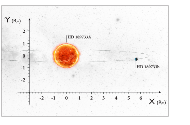
Figure 1.— Artist representation of the exoplanet HD 189733b. HD 189733b orbits in nearly circular motion around its host-star HD 189733A; its orbital plane is parallel within about 4^∘ of the Earth-primary line of sight. Note the limb brightening effect emerging from the optically thin, stellar corona.

2. Modeling the HD 189733A corona and the HD 189733b atmosphere

Probing the gases and plasmas that form exoplanet atmospheres is a challenging task, as extra-solar bodies are usually very faint. Yet, constraints on the atmospheric composition and temperature of the external layers of hot Jupiter and hot Neptune-like planets can be derived from primary and secondary eclipses for transiting exoplanets (Seager & Sasselov, 2000). Numerical models are thus very useful to evaluate the detection capabilities of our current and forthcoming generation of telescopes, together with fitting observed spectra with atmospheric models. It is in this scope that we now present a planetary system model for HD 189733 derived from observations. A sketch of our model is presented in Fig. 1. We list in Tab. 1 the physical properties of HD 189733A and HD 189733b that we use in this work. Note that our results are likely to vary if a new set of input parameters is derived from future observations.

2.1. Template X-ray spectrum of the HD 189733A quiescent corona

Table 1Physical properties of HD 189733A and HD 189733b

Property	Value	Reference
$R_{\star}/R_{\odot}$	$0.756\pm 0.018$	Torres, Winn & Holman (2008)
$M_{\star}/M_{\odot}$	$0.806\pm 0.048$	Torres, Winn & Holman (2008)
$R_{\mathrm{p}}/R_{\star}$	$0.15463\pm 0.00022$	Torres, Winn & Holman (2008)
$R_{\mathrm{p}}/R_{\mathrm{J}}$	$1.138\pm 0.027$	Torres, Winn & Holman (2008)
$M_{\mathrm{p}}/M_{\mathrm{J}}$	$1.144^{+0.057}_{-0.056}$	Torres, Winn & Holman (2008)
$a$/au	$0.03099^{+0.00060}_{-0.00063}$	Torres, Winn & Holman (2008)
$R_{\mathrm{Roche}}/R_{\mathrm{p}}$	4.35	Salz et al. (2016)
$P/\mathrm{days}$	$2.21857312^{+0.00000036}_{-0.00000076}$	Triaud et al. (2009)
$d/\mathrm{pc}$	19	Bouchy et al. (2005)
$i_{\mathrm{orbit}}/\mathrm{deg}$	$85.58\pm 0.006$	Torres, Winn & Holman (2008)
$b$	$0.680\pm 0.005$	Torres, Winn & Holman (2008)

The moderately active corona of HD 189733A emits X-ray photons from an optically thin plasma in collisional ionization-equilibrium; the X-ray spectrum is a bremsstrahlung continuum emission plus line emission from metals. The X-ray spectra of the quiescent corona obtained with XMM-Newton and Chandra are well described by two-isothermal plasma (Pillitteri et al., 2010, 2011, 2014; Poppenhaeger et al., 2013). Each isothermal plasma is characterized by an electronic temperature and a corresponding emission measure, defined as $EM=\int n_{\mathrm{e}}^{2}dV$ for a fully ionized plasma where the electronic density, $n_{\mathrm{e}}$, is equal to the ion density. The photoelectric absorption above 0.2 keV along the line of sight is negligible since the distance of this star is low.

We use the spectral fitting parameters of the quiescent corona obtained on April 17, 2007 with XMM-Newton by Pillitteri et al. (2011) for a distance of $d=19.3$ pc: a cool plasma component with $kT_{1}=0.24\pm 0.01$ keV (corresponding to $T_{\mathrm{e,1}}=2.8\pm 0.1$ MK) and $EM_{1}=4.7_{-0.3}^{+0.4}\times 10^{50}$ cm^-3, and warm plasma component with $kT_{2}$=0.71${}_{-0.03}^{+0.04}$ keV (corresponding to $T_{\mathrm{e,2}}=8.2_{-0.3}^{+0.5}$ MK) and $EM_{2}=(2.8\pm 0.3)\times 10^{50}$ cm^-3.

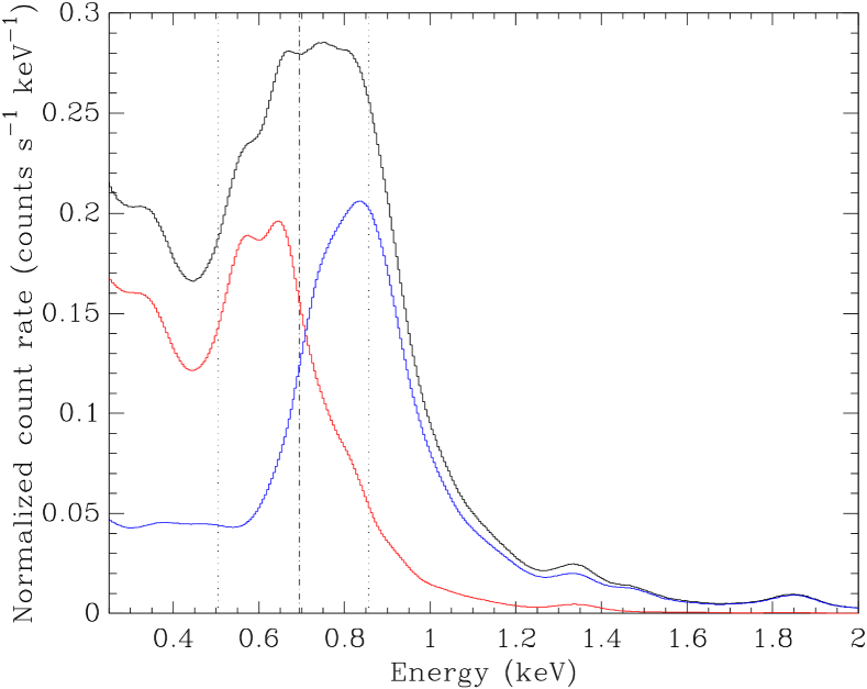
Figure 2.— XMM-Newton/pn template spectrum of HD 189733A used in this work. The energy range is 0.25–2 keV. Top panel: instrumental spectrum simulated from X-ray observations, grouped with a minimum of 25 counts. The dashed-dotted and dotted vertical lines are the energies of the median (50th-percentile), lower and upper quantiles (25th and 75th-percentiles) of the observed count rates, respectively. The red, blue, and black lines are the cool, warm, and total plasma components, respectively. Bottom panel: unfolded spectrum. The red, blue, and black dots are the cool, warm, and total plasma components used for our modeling of the X-ray corona, respectively.

We model this quiescent coronal emission with XSPEC (version 12.9.0) using two vapec models (Smith et al., 2001) with element abundances of Anders & Grevesse (1989) and Fe=0.57, O=0.51, and Ne=0.3 (Pillitteri et al., 2011). We simulate an XMM-Newton observation of this coronal model with the European Photon Imaging Camera (EPIC) pn instrument (Strüder et al., 2001) and the medium filter (Strüder et al., 2001) which determines in the 0.25–2.0 keV energy range an X-ray flux of $2.9\times 10^{-13}$ erg.cm^-2.s^-1 (corresponding to an X-ray luminosity of $1.3\times 10^{28}$ erg.s^-1 for $d$=19.3 pc) with a count rate of 0.188 pn count s^-1.

The count rate distribution versus energy, i.e., the simulated instrumental spectrum, is shown in the top panel of Fig. 2. Among the total counts detected in the 0.25–2.0 keV energy range, 25% have energy lower than 0.51 keV (see lower dotted vertical line), 50% have energy lower than 0.69 keV (see lower dashed-dotted vertical line), 75% have energy lower than 0.86 keV (see upper dotted vertical line). The bottom panel of Fig. 2 is the so-called unfolded spectrum with an energy sampling of $\sim$5 eV.

We will use this template spectrum to compute numerically the depth of the transit observed in the 0.25–2 keV energy range with XMM-Newton (Sect. 2.4).

We will perform in Sect. 2.5 Monte-Carlo radiative transfer simulations at the mean energy of the photons detected in the 0.25-2 keV energy band, $E_{\mathrm{mean}}=0.70$ keV, where the X-ray emission is mainly bremsstrahlung continuum emission. The coronal photon flux at this energy is $11.8\times 10^{-5}$ photons cm^-2 s^-1, with $F_{\mathrm{ph,1}}=9.2\times 10^{-5}$ and $F_{\mathrm{ph,2}}=2.6\times 10^{-5}$ photons cm^-2 s^-1, the photon flux from the cool and warm plasma, respectively (bottom panel of Fig. 2). We will assess the impact on the transmitted flux of X-ray observation in a broad energy-band in Sect. 2.4.3.

2.2. Model of the HD 189733 quiescent corona

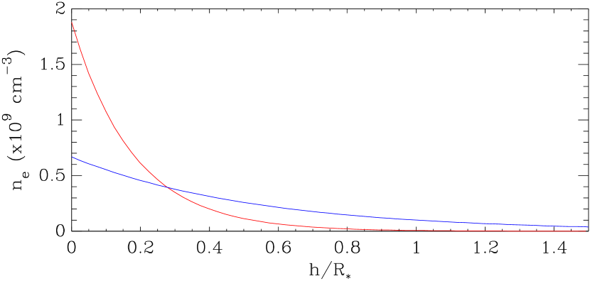
Figure 3.— Coronal electronic density versus the height above the corona. The red and blue lines are for the cool and warm coronal plasma, respectively.

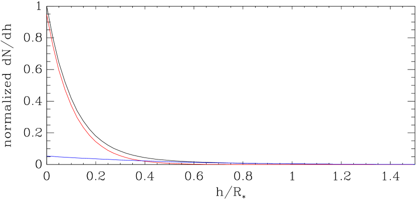
Figure 4.— Ratio of warm-to-cool plasma emissivity (with identical normalization) versus energy. The cross is the value corresponding to $E_{\mathrm{mean}}=0.7$ keV (vertical dashed line).

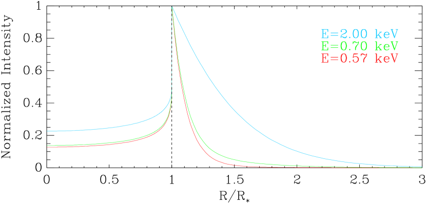
Figure 5.— Normalized photon emission at $E_{\mathrm{mean}}=0.7$ keV versus the height above the corona. The red and blue are for the cool and warm coronal plasma, respectively. The solid line is for the cool+warm coronal plasma and is normalized at the peak.

Figure 6.— Coronal emission profile integrated along the line of sight versus the distance from the stellar center. The vertical dashed line is the solar limb. All the profiles have been normalized at the solar limb (vertical dashed line). The red and blue lines are the most compact and extended coronal emission profiles occuring at 0.57 and 2.00 keV, respectively. The green line is the coronal emission profile at 0.7 keV that we use in our simulation.

The X-ray emitting plasma of the Sun corona is visible both in active regions where it is confined in magnetic loops and in the most homogeneous parts of the quiet Sun corona where there is any detectable features of magnetic loops; both coronal regions extending well above the photosphere. For HD 189733A only the large-scale magnetic topology is accessible from Zeeman-Doppler imaging, Moutou et al. (2007) showed that “it is significantly more complex than that of the Sun ; it involves in particular a significant toroidal component and contributions from magnetic multipoles of order up to 5”. However, it is beyond the scope of this article to use this magnetic topology as a scaffold to build a model of the X-ray emitting plasma of the HD 189733A corona (see, e.g., Jardine et al. 2006). We focus on the quiescent and diffuse corona, which is more representative of the average plasma distribution on the stellar surface. Therefore, following our template spectrum, we model the quiescent corona as two isothermal-plasma in hydrostatic equilibrium (see Sect. 3.3 of Aschwanden 2004).

In the isothermal approximation, the pressure scale height is defined as:

$$\lambda_{\mathrm{p}}(T_{\mathrm{e}})=\frac{2kT_{\mathrm{e}}}{\mu m_{\mathrm{H}}g_{\star}}\,,$$ (1)

where $k$ is the Boltzmann’s constant, $\mu\approx 1.27$ is the mean particle weight, $m_{\mathrm{H}}$ is the mass of the hydrogen atom, and $g_{\star}=GM_{\star}/R_{\star}^{2}$ is the stellar gravitational field. For HD 189733, we obtain: $\lambda_{\mathrm{p}}(T_{\mathrm{e}})=3.4\times 10^{9}\times(T_{\mathrm{e}}/\mathrm{MK})$ cm. Therefore, $\lambda_{\mathrm{p}}(T_{\mathrm{e,1}})=0.18R_{\star}$ and $\lambda_{\mathrm{p}}(T_{\mathrm{e,2}})=0.53R_{\star}$. Since the pressure is obtained by $p=2n_{\mathrm{e}}kT_{\mathrm{e}}$, the electronic density scale height is identical to the pressure scale height in the isothermal approximation. Neglecting the variation of the gravitational field with the height above the photosphere, $h$, the electronic density, $n_{\mathrm{e}}$, follows an exponential profile:

$$n_{\mathrm{e}}(h)=n_{\mathrm{e}}(0)\exp{\!\left\{\frac{-h}{\lambda_{\mathrm{p}}(T_{\mathrm{e}})}\right\}}\,.$$ (2)

We introduce, $f_{\mathrm{obs}}$, the fraction of the corona outer area that is not eclipsed by the stellar disk for an observer on Earth (Eq. 5 of Schmitt 1990):

$$f_{\mathrm{obs}}(x)=0.5\times\frac{1+\sqrt{x(2+x)}}{1+x}\,,$$ (3)

with $x=h/R_{\star}$. Obviously, only half of the coronal area is visible when $h=0$ ($f_{\mathrm{obs}}(0)=0.5$), and the coronal area is fully visible when $h=\infty$ ($f_{\mathrm{obs}}(\infty)=1.0$).

The observed emission measure must be computed on the coronal volume that is not eclipsed by the stellar disk:

$$EM_{\mathrm{obs}}=\int_{0}^{\infty}\frac{dEM(h)}{dh}f_{\mathrm{obs}}\!\left(\frac{h}{R_{\star}}\right)\,dh\,,$$ (4)

with the differential emission measure

$$\frac{dEM(h)}{dh}=n_{\mathrm{e}}(h)^{2}4\pi(R_{\star}+h)^{2}\,.$$ (5)

From Eq. 1–5 and the values of the observed electronic temperatures and emission measures, we derive numerically the electronic density at the base of the corona: $n_{\mathrm{e,1}}(0)=1.9\times 10^{9}$ cm^-3 and $n_{\mathrm{e,2}}(0)=6.7\times 10^{8}$ cm^-3; Fig. 6 shows the corresponding profiles of the coronal electronic density.

We obtain the profile of the photon number emitted by the corona for an energy, $E$, and a height, $h$, above the corona:

$$\frac{dN(E_{i},h)}{dh} = \Delta E_{i}\times\frac{10^{-14}}{4\pi d^{2}}\times{\tt vapec}(E_{i},kT_{1})\times$$ (6)

$$(\frac{dEM_{1}(h)}{dh}$$

$$+\frac{{\tt vapec}(E_{i},kT_{2})}{{\tt vapec}(E_{i},kT_{1})}\times\frac{dEM_{2}(h)}{dh})\,,$$

where $\Delta E_{i}$ is the width of the spectral bin of the ancillary response file at energy $E_{i}$, and ${\tt vapec}(E_{i},kT_{j})$ is the X-ray photon flux (in unit of photons cm^-2 s^-1 keV^-1) for a plasma temperature of $kT_{j}$ and a normalization of 1 (i.e., ${\tt vapec}$ parameter $norm\equiv 10^{-14}EM/4\pi d^{2}=1$).

The ratio of warm-to-cool plasma emissivity in Eq. 6 is plotted versus the energy in Fig. 6, using the energy sampling of the unfolded spectrum. Peaks and dips are due to emission lines from the warm and cool plasma, respectively. In the 0.25-2 keV energy band, the minimum and maximum values are 0.06 and 262 achieved at 0.57 and 2.00 keV, respectively. For a spectral energy resolution of $\Delta E_{i}=5$ eV, ${\tt vapec}(E,kT_{2})/{\tt vapec}(E,kT_{1})$ is equal to 0.45 at $E=E_{\mathrm{mean}}=0.7$ keV. Figure 6 shows the resulting normalized profile of the photons emitted by the corona at $E_{\mathrm{mean}}$ obtained using Eq. 6. Figure 6 shows the corresponding emission intensity integrated along the line of sight versus $R$, the distance from the stellar center. The emission intensity is maximum at the stellar limb and decreases from it with the distance, more or less slowly depending of the small or large contribution, respectively, of the warm plasma compared to the cool plasma to the coronal emission. Therefore, the size of the coronal emission varies with energy: the smallest and largest sizes are observed at 0.57 and 2.00 keV, respectively.

We define the quiescent corona has layers of constant, isotropic, and optically thin emission, above an optically thick sphere of radius $R_{\star}$ (Fig. 6). Since ordinary bremsstrahlung emission from plasma shows no intrinsic polarization due to the random motions of electrons (Dolan, 1967), we consider only unpolarized X-ray photons from the stellar corona.

2.3. Model of the HD 189733b atmosphere

The physical properties of the upper atmosphere of HD 189733b can be constrained with transmission spectroscopy of HD 189733A (for a review of exoplanetary atmospheres see Madhusudhan et al., 2014). Assuming that the transmission spectrum of HD 189733A from optical to near-infrared is dominated by Rayleigh scattering, Lecavelier Des Etangs et al. (2008) derive an atmospheric temperature of $1340\pm 150$ K at 0.1564 $R_{\star}$. They prefer scattering by condensates of Enstatite (MgSiO₃, with radius between $\sim 10^{-2}$ and $\sim 10^{-1}$ $\mu$m) rather than by molecular hydrogen. Assuming solar abundances, they derive at 0.1564 $R_{\star}$ for particle sizes of about $10^{-2}$ – $10^{-1}$ $\mu$m, a pressure of $2\times 10^{-3}$–$2\times 10^{-6}$ bar and a particle density of $1.1\times 10^{16}$–$1.1\times 10^{13}$ cm^-3. The revised transmission spectrum across the entire visible and infrared range is well dominated by Rayleigh scattering, which is interpreted as the signature of a haze of condensed grains extending over more than two orders of magnitude in pressure, with a possible gradient of grain sizes in the atmosphere due to sedimentation processes (Pont et al., 2013).

The gas of the HD 189733b atmosphere is photoionized by the UV emission of HD 189733A (e.g., Sanz-Forcada et al., 2011) and cools by radiation from collisionally excited atomic hydrogen, which leads similarly to H ii regions to a temperature of about $10,000$ K. This high temperature produces a (slow) evaporative-wind (Yelle, 2004; Murray-Clay et al., 2009).

Figure 7.— Atmospheric model of HD 189733b of Salz et al. (2016) used in our X-ray simulation. From top to bottom panels, the total Hydrogen number density, temperature, pressure, velocity, and Hydrogen (green) and Helium (red) ionic fractions of the planetary atmosphere are represented versus the distance from the planetary center, ranging from the planetary radius to the Roche’s radius.

Huitson et al. (2012) detected an upper atmospheric heating of HD 189733b from HST sodium observations, i.e., evidence of a thermosphere. Salz et al. (2015) obtained a 1D, spherically symmetric hydrodynamic simulations of the escaping atmosphere of HD 189733b, predicting gas velocity of $\sim$9 km s^-1 at the Roche’s radius, $R_{\mathrm{Roche}}=4.35~{}R_{\mathrm{p}}$ (Fig. 7), by coupling a detailed photoionization and plasma simulation code with a general MHD code, and assuming only atomic Hydrogen an Helium in the atmosphere. Since the resulting temperature-pressure profile (see below Fig. 12) is consistent with the rise of temperature with the altitude observed by Huitson et al. (2012), we adopt the Salz et al. (2015)’s profiles to describe for $r\geq R_{\mathrm{p}}$ the thermosphere of HD 189733b.

Line et al. (2014) showed from secondary eclipse spectroscopy that for $R_{\mathrm{p}}\geq r\geq r_{\mathrm{in}}$, corresponding to an atmospheric pressure increasing from $p(R_{\mathrm{p}})\sim$10 to $p(r_{\mathrm{in}})\sim 1000$ dyn cm^-2, the lower atmosphere of HD 189733b is isothermal, with an equilibrium temperature of $T_{\mathrm{eq}}\sim 1200$ K. Therefore, we use the hydrostatic equilibrium to extent the pressure and density profiles into this lower atmospheric layer. The pressure scale height of this neutral atmospheric layer is:

$$\lambda_{\mathrm{p}}^{\mathrm{atm}}(T_{\mathrm{eq}})=\frac{kT\mathrm{eq}}{\mu(R_{\mathrm{p}})m_{\mathrm{H}}g_{\mathrm{p}}}$$ (7)

where $g_{\mathrm{p}}=GM_{\mathrm{p}}/R_{\mathrm{p}}^{2}$ is the planetary gravitational field, and $T_{\mathrm{eq}}=1190$ K and $\mu(R_{\mathrm{p}})=1.28015$ (Salz et al., 2016), which leads to $\lambda_{\mathrm{p}}^{\mathrm{atm}}(T_{\mathrm{eq}})=0.0043~{}R_{\mathrm{p}}$ (i.e., 350 km). The pressure and density follow the same exponential profile:

$$p(r) = p(R_{\mathrm{p}})\times f(r)$$ (8)

$$n_{\mathrm{H}}(r) = n_{\mathrm{H}}(R_{\mathrm{p}})\times f(r)$$ (9)

where

$$f(r)=\exp{\!\left\{-\frac{r-R_{\mathrm{p}}}{\lambda_{\mathrm{p}}^{\mathrm{atm}}(T_{\mathrm{eq}})}\right\}}$$ (10)

when neglecting the variation of the planetary gravitional field with the depth below the planetary radius, and $p(R_{\mathrm{p}})=12.7$ dyn cm^-2 and $n_{\mathrm{H}}(R_{\mathrm{p}})=7.7\times 10^{13}$ cm^-3 (Salz et al., 2016). Therefore, $r_{\mathrm{in}}=0.981R_{\mathrm{p}}$ and $n_{\mathrm{H}}(r_{\mathrm{in}})=6.0\times 10^{15}$ cm^-3.

2.4. Analytic computation of the transmitted flux

2.4.1 X-ray absorption radius

The planetary absorption radius during transit is defined as the distance in the plane of the sky from the planetary center where the optical depth through the atmosphere along the line-of-sight, $\tau$, is equal to unity. The total photon extinction cross-section in X-rays is the sum of photoelectric absorption and scattering cross-sections. The latter is the sum of coherent (Rayleigh) and incoherent (Compton) scattering by bound electrons in atoms/molecules (Hubbell et al., 1975). For comparison, we compute these cross-section components for an atmosphere of neutral Hydrogen and Helium with solar abundances (Asplund et al., 2009) with the XCOM (Berger & Hubbell, 1987). At 1 keV the total photon cross-section is 46.5 barn/H atom, composed at 98.1% by the photoelectric absorption (45.6 barn/H atom), this proportion decreases with higher energy. The scattering cross-section at 1 keV is dominated by the coherent (Rayleigh) process with 0.8 barn/H atom compared to 0.1 barn/H atom for the incoherent (Compton) scattering. Therefore, we will neglect the scattering cross-sections in our analytic computation at 0.7 keV.

The simplified solution of the absorption radius proposed by Fortney (2005) is only valid for a geometrically thin atmosphere and can not be used a priori here due to the extended evaporative-wind. From the geometrical parameters introduced in Fig. 8, the optical depth at energy $E$ through the planetary atmosphere along the line-of-sight is computed versus the distance from the planetary center, $r$, as follows:

$$\frac{\tau{{}_{\mathrm{X}}(r,E,Z)}}{2}=\!\!\int_{0}^{L}\!\!\!\sigma_{\mathrm{X}}(\sqrt{r^{2}+l^{2}},E,Z)\,n_{\mathrm{H}}(\sqrt{r^{2}+l^{2}})\,dl$$ (11)

with $L=\sqrt{R_{\mathrm{Roche}}^{2}-r^{2}}$, $n_{\mathrm{H}}$ the total Hydrogen number density, and $\sigma_{\mathrm{X}}(r,E,Z)$ the photoelectric cross-section per Hydrogen atom, where $Z$ is the metallicity.

Figure 8.— Definition of the geometrical parameters of the planetary atmosphere.

The photoelectric cross-section at the distance $r$ from the planetary center and energy $E$ is computed as:

$$\sigma_{\mathrm{X}}(r,E,Z) = f_{\mathrm{H}}(r)\,\sigma_{\mathrm{X,H}}(E)$$ (12)

$$+ A_{\mathrm{He}}\left(f_{\mathrm{He}}(r)\,\sigma_{\mathrm{X,He}}(E)+f_{\mathrm{He^{+}}}(r)\,\sigma_{\mathrm{X,He^{+}}}(E)\right)$$

$$+ Z\sum_{\mathrm{k\notin[H,He]}}\!\!A_{k}\,\sigma_{\mathrm{X,}k}(E)$$

with $f_{\mathrm{H}}$, $f_{\mathrm{He}}$, and $f_{\mathrm{He^{+}}}$ the ionic fractions (see bottom panel of Fig. 7); $A_{i}$ the abundance in number of the neutral element $i$ relative to the hydrogen (Asplund et al., 2009) and $\sigma_{\mathrm{X,}i}$ the photoelectric cross-section of the neutral or ionized element $i$ relative to the hydrogen (Verner & Yakovlev, 1995). Since the dust grains in the planetary atmosphere are optically thin to X-rays due to their small sizes ($\ll 1$ $\mu$m), there is no self-blanketing effect, i.e., no decrease of the X-ray cross-section due to some element in the solid phase (Bethell et al., 2011).

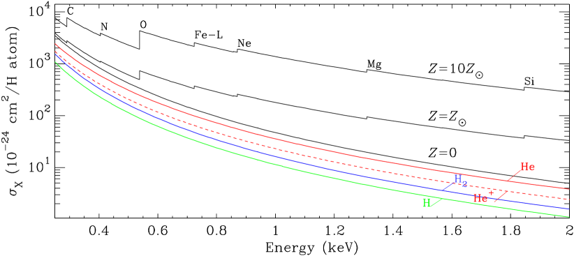
Figure 9.— Photon cross-section of photoelectric absorption in X-rays versus metallicity. The green and blue solid-lines are the X-ray cross-sections of atomic and molecular Hydrogen, respectively. The solid and dashed red-lines are the X-ray cross-sections of neutral and one-times ionized Helium, respectively. The black solid lines are the X-ray cross-section for neutral atomic Hydrogen and Helium with no metals, solar metallicity and ten times solar metallicity (no metallic ions). The main ionization-edges of the inner electronic-shells are labeled with element names and shell name except for K.

Figure 10.— Optical depth through the planetary atmosphere along the line-of-sight at $E_{\mathrm{mean}}=0.7$ keV versus the distance to the planet center. The planetary atmosphere is composed of atomic H, He and He⁺ with no metals, solar metallicity and ten times solar metallicity (no metallic ions). The vertical dotted lines indicate the corresponding X-ray absorption radius.

Following Salz et al. (2016), we will only consider in our simulation atomic Hydrogen and Helium photoelectric cross-sections (Fig. 10). Since $\sigma_{\mathrm{X,H_{2}}}=2.85\,\sigma_{\mathrm{X,H}}$ (Wilms et al., 2000) and $A_{\mathrm{H_{2}}}=0.5$, the contribution of the molecular Hydrogen in the low atmosphere to an increase of the photoelectric cross-section is small. However, metal abundances has a strong impact on the photoelectric absorption. Since ions (e.g., He⁺) have lower photoelectric cross-section than neutral elements (fully ionized elements have obviously a null photoelectric cross-section), the ionized escaping atmosphere is more transparent to X-rays than the lower atmosphere.

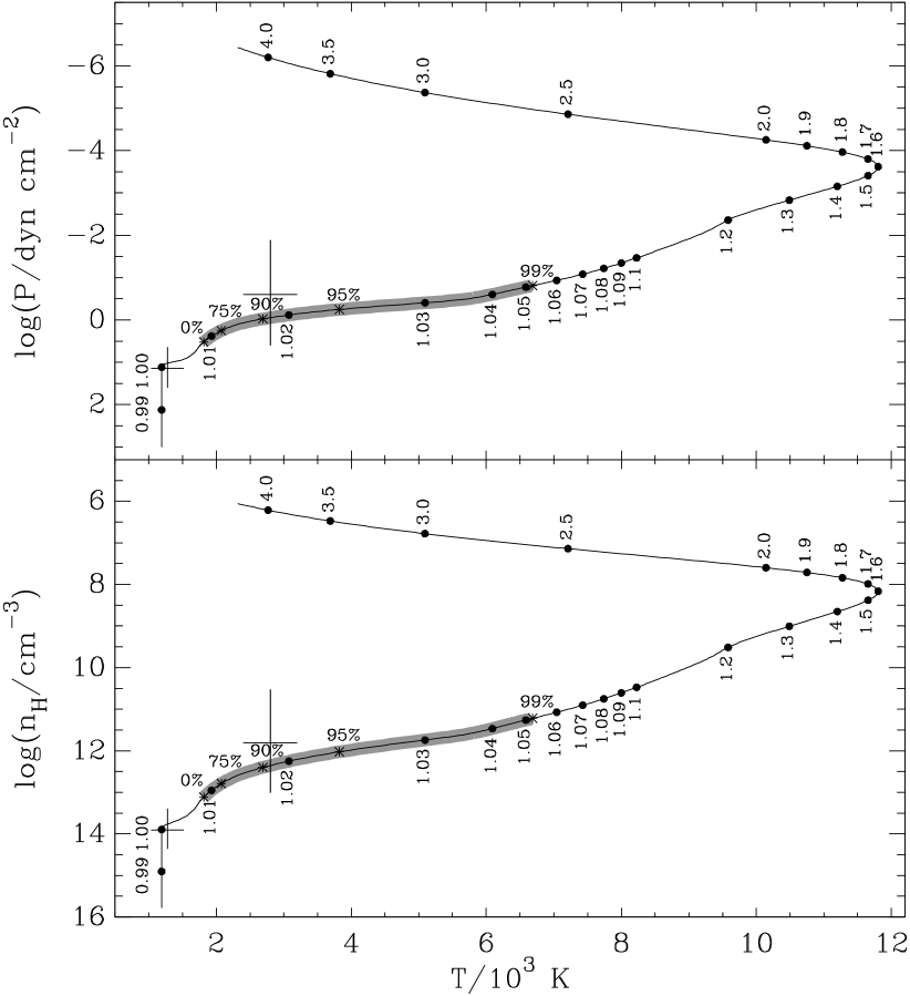
Figure 11.— Cumulative contribution of the atmosphere at elevation $z$ above the planetary radius to the optical depth at the X-ray absorption radius at 0.7 keV (vertical dashed line). The maximum elevation value on the x-axis corresponds to the atmospheric layer contributing for 99% to the optical depth.

Figure 12.— Atmospheric structure of HD 189733b (adapted from Salz et al. 2016). The top and bottom panels are the pressure-temperature and the density-temperature profile, respectively. The crosses are the HST Sodium observations of Huitson et al. (2012). The vertical labels give the distance from the planetary center in planetary radius. The thick grey region with percent-labeled asterisks indicates the contribution of the atmospheric layers to the absorption at the X-ray absorption radius at 0.7 keV (Fig. 12).

Figure 10 shows the variation of the optical depth (Eq. 12) at 0.7 keV versus the distance to the planetary center. We find that the planetary absorption radius at 0.7 keV, $R_{\mathrm{X}}(\mathrm{0.7~{}keV})$ is 1.008 $R_{\mathrm{p}}$ (corresponding to 0.156 $R_{\star}$), i.e., located at $z=$634 km above the planetary radius. Figure 12 shows that 99% of the absorption at $R_{\mathrm{X}}(\mathrm{0.7~{}keV})$ is produced by the upper ($z$=634–4243) atmospheric layers that intersect the line of sight (e.g., the dashed circle in Fig. 8). In this absorbing atmospheric shell with a width of 3,609 km the total Hydrogen number density and temperature ranges are $1.1\times 10^{13}$–$1.2\times 10^{11}$ cm^-3 and 1870–7004 K, respectively (Fig. 12). The physical properties of the atmospheric layers that contribute to the bulk of the X-ray absorption are constrained by the optical measurements of Huitson et al. (2012).

Assuming that adding metals in the atmosphere would not change dramatically the density-temperature profile (see, however, the discussion in Salz et al. 2016), we estimate that $R_{\mathrm{X}}(\mathrm{0.7~{}keV})$ increases from 1.008 to 1.059 $R_{\mathrm{p}}$ (or equivalently from 0.156 to 0.164 $R_{\star}$) when the neutral metals increase from zero to ten times the solar metallicity (Fig. 10).

2.4.2 Transmitted flux at 0.7 keV during the planetary transit on the stellar corona

For comparison purpose, we compute the phases of the first, second, third and fourth contacts of the primary eclipse in the optical: $\phi_{1}=-\phi_{4}=-0.0169$ and $\phi_{2}=-\phi_{3}=-0.0091$ (vertical dotted lines in Fig. 13). The corresponding photospheric transit of a uniformly emitting disk (e.g., Mandel & Agol, 2002) has a maximum transit depth of $(R_{\mathrm{p}}/R_{\star})^{2}=2.39\%$ (dotted line in Fig. 13).

The chromospheric transit was computed analytically by Schlawin et al. (2010), assuming an optically thin and geometrically thin shell of emission (zero thickness). It is characterized by a W-profile with a maximum depth of approximately $\delta_{\mathrm{max,approx}}^{\mathrm{chrom}}=0.5(R_{\mathrm{p}}/R_{\star})^{3/2}$, i.e., $0.5(R_{\mathrm{p}}/R_{\star})^{-1/2}$ times deeper than the maximum transit depth of a uniformly emitting disk. These two minimums occur slightly before and after the second and third contacts, respectively, with a depth here of exactly $\delta_{\mathrm{max}}^{\mathrm{chrom}}=3.10\%$ (dashed line in Fig. 13). This characteristic shape is due to the strong limb brightening that occurs since the zero-thickness chromosphere has its largest column density at the disk’s edge.

We compute numerically the normalized light curve of the planetary transit on the stellar corona from the coronal emission profile integrated along the line of sight, $I$ (Fig. 6), and the optical depth through the planetary atmosphere, $\tau$ (Fig. 10), using the formula:

$$I_{\mathrm{transit}}(t)=\frac{\int_{-\infty}^{+\infty}\int_{-\infty}^{+\infty}I(\sqrt{X^{2}+Y^{2}})\,e^{-\tau\left(\frac{r(X,Y,t)}{R_{\mathrm{p}}}\right)}dXdY}{\int_{-\infty}^{+\infty}\int_{-\infty}^{+\infty}I(\sqrt{X^{2}+Y^{2}})\,dXdY}$$ (13)

where $X$ and $Y$ are the cartesian coordinates in the plane of the sky expressed in stellar radius (Fig. 1), and $r(X,Y,t)=\sqrt{(X-X_{\mathrm{p}}(t))^{2}+(Y-Y_{\mathrm{p}}(t))^{2}}$ is the distance from the position of the planetary center at time $t$, $X_{\mathrm{p}}(t)=a\cos(i)\sin(2\pi t/P)$ and $Y_{\mathrm{p}}(t)=-a\cos(i)\cos(2\pi t/P)$. We obtain a similar W-profile since the coronal emission is also optically thin (solid line in Fig. 13). But, the coronal transit is less deep and more extended than the chromospheric transit since the corona is extended above the photosphere (green line in Fig. 6). We find $\delta_{\mathrm{max}}=2.06\%$ at $\phi=\pm 0.0143$, corresponding to a temporal shift of $\pm$45.8 min from the transit center. At the transit center the depth is reduced to only 0.77%.

Figure 13.— Light curves of the planetary transits of HD 189733b. The black solid line is the coronal transit at 0.7 keV computed for $R_{\mathrm{X}}(\mathrm{0.7~{}keV})=1.008R_{\mathrm{p}}$ (corresponding to a planetary atmosphere of H, He, and He⁺). For comparison, the vertical dotted lines indicated the first, second, third, and fourth contacts of the photospheric transit in the optical. The dotted and dashed lines are the photospheric transit (uniformly emitting disk, e.g., Mandel & Agol 2002) and the chromospheric transit (Schlawin et al., 2010), respectively. The cross data are the coronal transit signature obtained by our simulation at 0.7 keV (see Fig. 17).

2.4.3 Impact of the broad energy-band on the observed transmitted flux

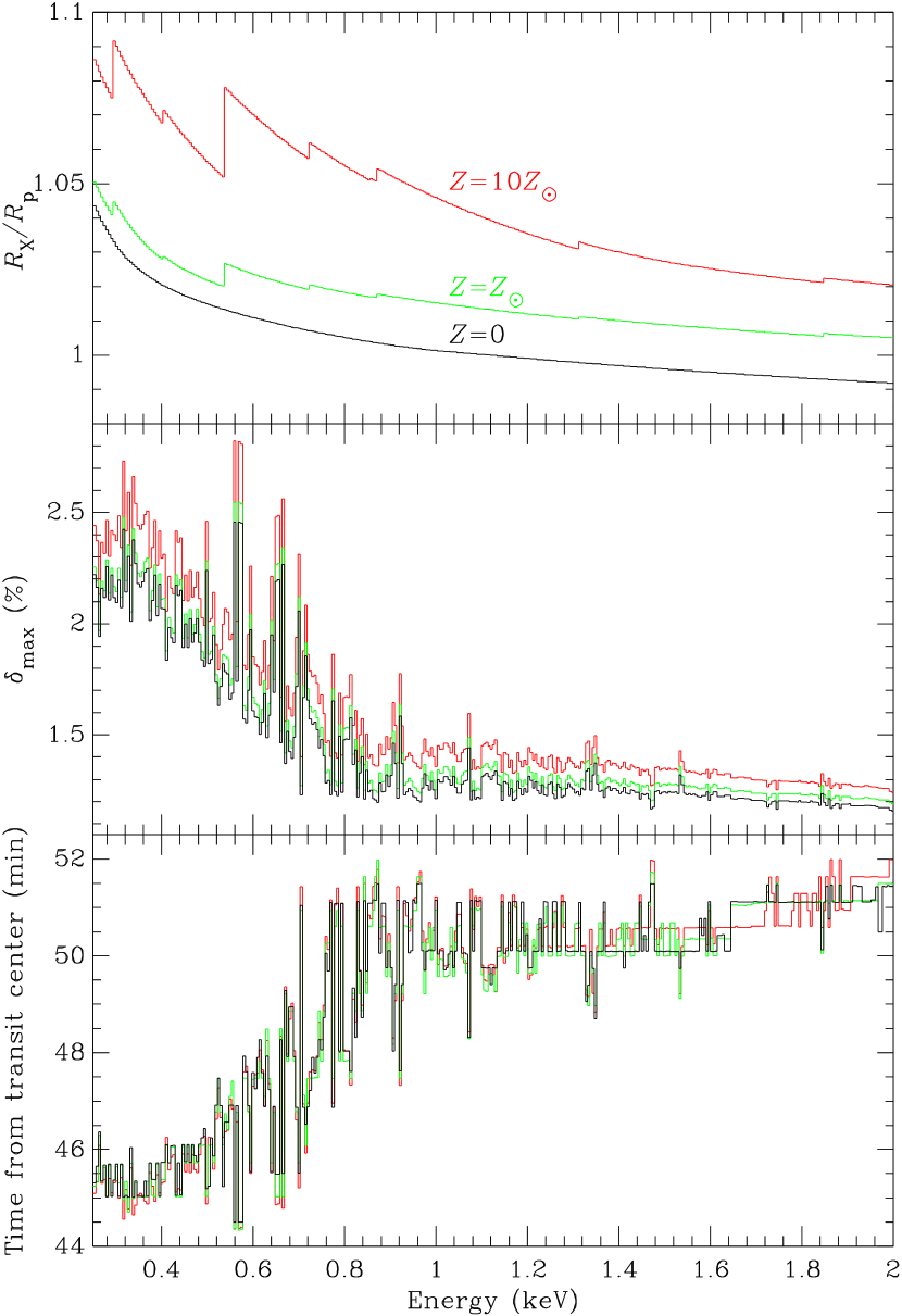
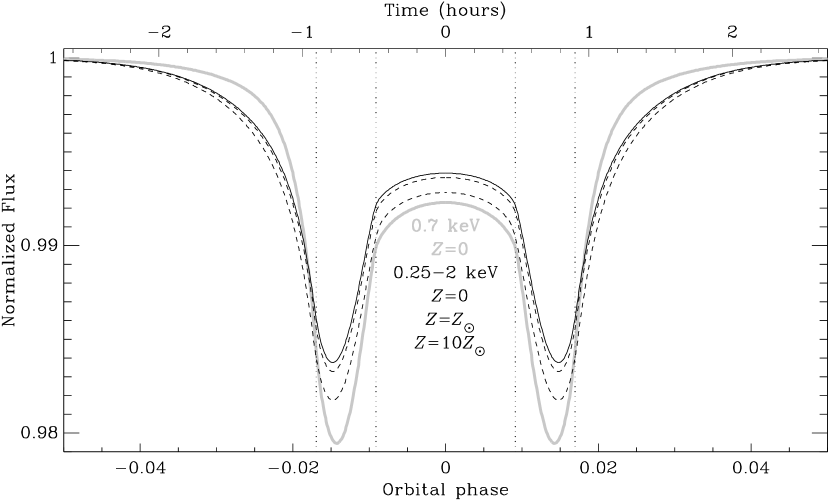
Figure 14.— Characteristics of the coronal transit versus X-ray energy. Top panel: X-ray absorption radius given in planetary radius. Middle panel: maximum depth of the coronal transit in percent. Bottom panel: temporal shift of the maximum depth from the transit center. Black, green, and red lines are for a planetary atmosphere composed of atomic H, He, He⁺ with no metals, solar metallicity and ten times solar metallicity (no metallic ions), respectively.

Figure 15.— Planetary transit in the 0.25–2.0 keV energy band. For comparison purpose, the vertical dashed lines are the eclipse contact in the optical and the grey line is the planetary transit at 0.7 keV for no metals.

Due to the limited sensitivity of the current X-ray facilities, any tentative detection of planetary transits must use light curves in a broad energy band to increase the signal-to-noise ratio. The extension and depth of the coronal transit is modified by the variations with energy of the coronal emission profile, the photon extinction cross-section (determining the absorption radius), and the observed stellar flux. It is therefore important to assess in a broad energy band the effective transit. This effective transit is the weighted average of the monoenergetic transit on the broad energy-band, using the observed X-ray count rate versus energy (i.e., the observed X-ray spectrum; top panel of Fig. 2) as weight.

For a given metallicity, we compute at each grid energy the coronal profile and the absorption radius, and the corresponding light curve of the coronal transit. The top panel of Fig. 15 shows the absorption radius decreasing with the energy, with local jump associated to the ionization edges of metals. When there is no metals, the X-ray absorption radius becomes lower than the planetary radius –the lower boundary of Salz et al. (2016)’s simulation– at energies larger than $\sim$1.1 keV. Therefore, the optical depth used to compute the absorption factor in Eq. 13 has also to be estimated inside the lower atmosphere, which requires an extension of the density model as we did in Sect. 2.3. This leads for comparison at $r_{\mathrm{in}}$ to $\tau(Z=0,E=2.0~{}\mathrm{keV})\sim 12$.

The mid and bottom panels of Fig. 15 show the maximum depth of the coronal transit and its temporal shift from the transit center, respectively, vs. energy. Both values are mainly correlated with the warm-to-cool plasma emissivity ratio (Fig. 6) that controls the extension of the corona.

Then, we compute the weighted average light curve of the coronal transit in the 0.25–2 keV energy band for XMM-Newton/pn using the template instrumental spectrum of HD 189733A as weight (Fig. 15). We obtain maximum transit depths of 1.62%, 1.67%, and 1.82%, for no metals, and one and ten times solar metallicity (no metallic ions), respectively, at $\phi=\pm 0.0148$ corresponding to a temporal shift of $\pm$47.4 min from the transit center; at the transit center the depth is reduced to 0.61%, 0.64%, and 0.72%, respectively.

Therefore, the maximum transit depth in the 0.25–2 keV energy band is little sensitive to the metal abundance. Moreover, the transit light curve at 0.7 keV (grey line in Fig. 15) is a correct approximation of the transit light curve in the 0.25–2 keV energy band.

2.5. Monte Carlo radiative transfer

To simulate the transit of HD 189733b in front of its host star, we used the radiative transfer code stokes. Originally written for polarimetric investigations of active galactic nuclei, stokes has been extended over the last years to cover a much larger panel of astrophysical sources (a detailed list of examples can be found in Marin & Goosmann 2014). The code and its characteristics are extensively described in Goosmann & Gaskell (2007), Marin et al. (2012) and Marin et al. (2015) for the optical/UV part, and in Marin & Dovčiak (2015) for the X-ray band, so we will simply summarize the principal aspects of stokes relevant for our computations.

The code can handle a large panel of emitting, scattering and/or absorbing geometries in a fully three-dimensional environment. Multiple scattering enables the code to radiatively couple all the different regions of a given model, and a web of virtual detectors arranged in a spherical geometry is used to record the photon wavelength, intensity, and polarization state, according to the Stokes formalism ($\vec{S}=(I,Q,U,V)^{\rm T}$). About 10¹¹ photons have been sampled for our analysis. The total intensity (flux), polarization degree $P$ (= $\sqrt{Q^{2}+U^{2}+V^{2}}/I$), and polarization angle $\psi$ (= $0.5\tan^{-1}(U/Q)$) are computed by averaging all the detected photons, at each line-of-sight in polar and azimuthal directions. Mie, Rayleigh, Thomson, Compton and inverse Compton scattering are included from the near-infrared to hard X-ray bands.

For planetary atmospheres in the X-ray domain, Rayleigh and Compton scattering of photons onto bound electrons will be the major mechanism to alter the net polarization, and a visual representation of the integrated and differential scattering cross sections produced by stokes is presented in Fig. 16. Note that for molecular hydrogen the incoherent scattering cross-section is two-times larger than for atomic hydrogen (Sunyaev et al., 1999).

Photo-ionization and recombination effects, which also influence the resulting polarization by absorption and unpolarized re-emission processes, are based on quantum mechanics computations from Lee (1994) and Lee et al. (1994). We use fluorescent yields and energy of the subsequently re-emitted Auger photons from the Opacity Project (Cunto & Mendoza, 1992), and X-ray photoelectric cross-sections and inner-shell edge energies of Verner & Yakovlev (1995). Finally, we opt for elemental abundances from Asplund et al. (2009) and ten times solar metallicity to allow direct comparison with Poppenhaeger et al. (2013).

Since the X-ray scattering by dust grains (Mathis & Lee, 1991) is not yet implemented in stokes, we consider only gaseous components. We do not consider additional soft X-ray emission from the exoplanet itself induced by the stellar wind charge exchange mechanism since it was estimated in the case of the close-in exoplanet HD 209458b to be about five orders of magnitude fainter than the emission from the host star (Kislyakova et al., 2015).

We divide our two-zone model with constant-density shells sampling any 0.1-dex variation of the density from a density of 7.697$\times$10¹³ cm^-3 corresponding to a pressure of 12.739 bar, a temperature of 1190.2 K, and a 0.7 keV optical depth of $\sim$4.608.

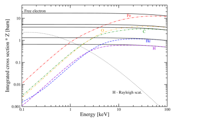
Figure 16.— Elemental photon scattering cross-section versus energy. Top: integrated cross-section for Compton scattering onto a variety of elements chosen accordingly to Asplund et al. (2009) for their high abundance. Solid black line: coherent (Compton) scattering on free electrons (Klein-Nishina cross-section). Incoherent (Compton) scattering on bound electrons: long-dashed violet line of H, short-dashed blue line of He, dot-short-dashed green line of C, double-dot-dashed orange line of O, dot-long-dashed red line of Fe. The black dotted line shows coherent (Rayleigh) scattering onto an hydrogen atom for comparison. Bottom: $E_{\mathrm{mean}}=0.7$ keV differential cross section versus scattering angle for the same free and bound electrons.

3. Photo-polarimetric results

We present the outcomes of our simulations in Fig 17. Results are plotted with respect to the orbital phase of HD 189733b, also converted into transit hours. Each data-point is associated with its 1$\sigma$ Monte Carlo error bars resulting from the simulation. The Monte Carlo statistical error is estimated using the standard deviation $\sigma$ that is roughly proportional to $\sqrt{\rm Var(X)}$/$\sqrt{N}$ for large $N$, with $N$ the number of photons sampled in the direction of the observer and Var(X) the variance of the estimate.

3.1. Photometry

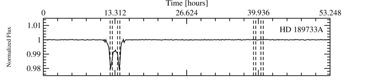
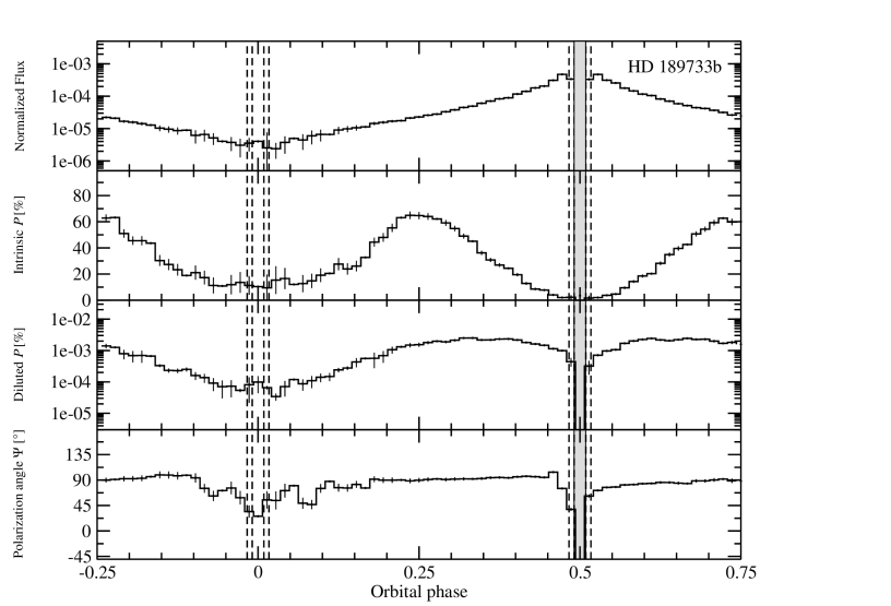
Figure 17.— Photometry at $E_{\mathrm{mean}}$=0.7 keV of HD 189733A, and reprocessed flux from the surface of HD 189733b (first two panels). The fluxes are normalized to the initial flux of the star. Polarimetric results are shown in terms of $P$ (polarization percentage) and $\psi$ (polarization position angle, defined with respect to the vertical axis of the system). The error bars correspond to 1$\sigma$ statistical errors in the Monte Carlo simulation. The vertical dashed lines are the first, second, third and fourth contacts of the primary (planetary transit) and secondary eclipses in the optical. The gray box indicates a region where polarization measurement of HD 189733b is impossible due to the disappearance of the exoplanet behind its star.

The top panel of Fig 17 shows the light curve of HD 189733A at 0.7 keV, normalized to unity. The exoplanet orbits in front of HD 189733A from orbital phase -0.25 to orbital phase +0.25, with an eclipse of the stellar corona (i.e., a planetary transit) occuring between orbital phases -0.0169 and +0.0169. During this planetary transit, the 0.7 keV flux decreases by 2.00$\pm$0.15 % between the first and second contacts, as the exoplanet starts to cover the X-ray corona, then rises to 1.07$\pm$0.15 % at orbital phase 0. It then decreases back to 2.02$\pm$0.15 % between the third and fourth contacts before resuming to the non-eclipsed flux, showing no more variation during the remainder of the orbit of HD 189733b. A close up representation of the transit is shown in Fig. 13 for clarity purposes. We find a perfect agreement between numerical and simulation results within the Monte-Carlo statistical error of our modeling.

Using the stokes code, we isolated photons that are re-emitted/scattered from HD 189733b, and plotted the resulting light curve (normalized with respect to the unitary flux of HD 189733A) in Fig 17 (second panel from the top). To increase the statistics of the photon-starved results, the phase resolution of the re-emitted/scattered radiation has been decreased compared to Fig. 13. Due to the strong photoelectric absorption processes that prevail at soft X-ray energies, the X-ray flux from the exoplanet is found to be three to five orders of magnitude lower than the photon flux from the main star. From the HD 189733A flux of $2.9\times 10^{-13~{}}$ erg cm^-2 s^-1 at 0.7 keV, the flux of HD 189733b is about $10^{-16}$ – $10^{-18}$ erg cm^-2 s^-1, depending on the orbital phase of the planet. The flux reprocessed onto the atmospheric layers of HD 189733b strongly depends on the angle between the source, the exoplanet atmosphere and the observer; this effect is due to the differential scattering phase function of incoherent scattering, as presented in Fig. 16 (bottom). In the case of Rayleigh scattering, forward and backward reprocessing prevails while, for incoherent scattering onto bound electrons, forward and perpendicular scattering are less probable. However, backscattering is very strong and when the gaseous planet passes beyond the plane-of-the-sky, its reprocessed flux rises up to a normalized flux of $\sim$ 4.7 $\times$ 10^-4. Then, HD 189733b disappears behind its star and flux drops to zero.

3.2. Polarization

The middle panel of Fig 17 is a visualization of the linear continuum polarization degree $P$, ranging from 0 (unpolarized) to 100 % (fully polarized). It is the polarization resulting from scattered light only, i.e. not diluted by the unpolarized stellar flux. The shape of the polarization curve is very similar to the results obtained by Stam et al. (2004), who evaluated the spectra of visible to near-infrared starlight reflected by Jupiter-like extrasolar planets. As Stam et al. (2004), we find polarization maximums close to orbital phases $\pm 0.25$, i.e., near planetary greatest elongations, with $P$ = 64.9$\pm$2.9 % which is slightly larger than in infrared. Since the planet’s orbital plane is inclined by 4^∘, the polarization degree does not drop to zero at zero orbital phase as a small fraction of photons scatters onto the top of the atmospheric layers towards the Earth. Hence, we are sure that our model produces correct results and extends the near-infrared/optical investigation of Stam et al. (2004) to X-ray energies.

The fourth panel of Fig 17 also shows the star+planet linear polarization, now taking into account polarization dilution by the unpolarized stellar photons, i.e., $P_{\mathrm{diluted}}=\sqrt{Q^{2}+U^{2}+V^{2}}/(I_{\star}+I_{\mathrm{p,scatt}})$. The overall shape of the polarization curve, associated with a polarization degree below 0.003 %, is quite different from the intrinsic $P$. In fact, maximum polarization is found when the exoplanet transits behind the plane-of-the-sky, with a local diminution to zero when HD 189733b is occulted by its primary star. The departure from a purely sinusoidal waveform is again due to the scattering phase function of incoherent scattering that promotes backscattering. Associated with maximum fluxes from HD 189733b that are not located at maximal planetary elongations, the net diluted polarization degree peaks at orbital phases +0.35 and +0.65. The highest degrees of $P$ are of the order of 0.0025 $\pm$ 0.0002 % at 0.7 keV, similarly to the polarization found in the optical band (Carciofi & Magalhães, 2005).

Finally, the bottom panel of Fig 17 presents the absolute polarization position angle $\psi$ to be observed with an X-ray polarimeter. When HD 189733b does not transit on HD 189733A, its polarization angle is equal to 90^∘ (the $\vec{E}$-vector of the radiation is aligned with the projected rotational axis of the orbit). However, when the planet is about to transit in front of its primary star, $\psi$ oscillates around 90^∘. The canceling contribution of unpolarized fluxes from the star and the 90^∘ oriented polarization position angle resulting from scattering prevent the $\psi$ value from stabilizing, resulting in a chaotic signal. This behavior is strengthened due to the edge-on orientation of the exoplanet’s orbit. As the illuminated side of HD 189733b, producing the scattering-induced polarization signal, is facing the star, an observer situated on Earth no longer detects the bright side of the atmosphere and the signal is almost canceled. Only photons that have scattered on the top of the atmosphere carry a non-random polarization signal. Since most of the radiation comes from HD 189733A, the resulting polarization signal is highly diluted and thus $\psi$ randomly oscillates.

Another variation of $\psi$ is detected when the planet passes behind HD 189733A: at the ingress (egress) point, the polarization position angle increases (decreases) by $\sim$ 30^∘, due to the partial obscuration of the reprocessing target. The inclination of the system and the partial obscuration of the planetary disk suppresses the averaging of polarization and results in $\psi$ variations before a pure cancellation of polarization due to the planet disappearance. The amplitude of the fluctuation of $\psi$ is directly correlated with the orbital inclination of the exoplanet and could be, in principle, used to estimate the impact parameter of the transit.

4. Is direct detection of the exoplanet in X-rays possible?

We presented the first quantification of the amount of X-ray flux reprocessed by the Hot Jupiter exoplanet HD 189733b, along with the first estimation of the net polarization a future X-ray polarimeter could detect.

4.1. Scattered X-ray flux

We find that the 0.7 keV flux of HD 189733b is three to five orders of magnitude lower than its primary main sequence K1.5 V star, depending on the orbital phase of the exoplanet. Considering a stellar flux of 2.9$\times$10${}^{-13~{}}$erg cm^-2 s^-1 at 0.7 keV and at a distance of 19.45 pc, it implies that the reprocessed flux from HD 189733b is lower than 1.0$\times$10${}^{-16~{}}$erg cm^-2 s^-1 at best before ingress and after egress.

Since the planetary emission cannot be spatially resolved from the stellar emission in X-rays (angular separation lower than $1\farcs 6$ mas), one can only look for flux modulation with orbital phase. As a guideline, we can use a threshold $f^{\mathrm{limit}}_{\mathrm{p}}$ of the planetary relative flux, $f_{\mathrm{p}}$, to divide the X-ray observation of $N$ planetary orbits (of period $P$ in seconds) in two parts. During the orbital phase $\Delta\phi$, where $f_{\mathrm{p}}$ is lower than $f^{\mathrm{limit}}_{\mathrm{p}}$, the X-ray count rate of HD 189733 is $CR_{\mathrm{low}}=<\!CR\!>(1+<\!f_{\mathrm{p}}\!>)$ with $<\!CR\!>$ the count rate of the host star and $<\!f_{\mathrm{p}}\!>$ the average planetary relative flux on $\Delta\phi$. During the orbital phase $1-\Delta\phi$, where $f_{\mathrm{p}}$ is larger than $f^{\mathrm{limit}}_{\mathrm{p}}$, the X-ray count rate of HD 189733 is $CR_{\mathrm{high}}=<\!CR\!>(1+\alpha<\!f_{\mathrm{p}}\!>)$, with $\alpha$ the average increase of the relative planetary flux. The increase of count rate $\Delta CR\equiv CR_{\mathrm{high}}-CR_{\mathrm{low}}$ is statistically significant if $\Delta CR\geq n\sigma$ with $n=4$ and assuming Poisson noise $\sigma^{2}=(CR_{\mathrm{low}}/\Delta\phi+CR_{\mathrm{high}}/(1-\Delta\phi))/(NP)$. Straightforward algebra leads to:

$$N\gtrsim n^{2}/(f^{2}(\alpha-1)^{2}\Delta\phi(1-\Delta\phi)P<\!CR\!>).$$ (14)

Using $<\!CR\!>=0.188$ pn count s^-1 (Sect. 2.1), we find a minimum value of $13,315$ orbits for $f^{\mathrm{limit}}_{\mathrm{p}}=7.5\times 10^{-5}$, $\alpha=8.7$, and $\Delta\phi=0.89$. Since the needed accuracy requires a total exposure time of 81 years, the modulation of the X-ray flux with the orbital phase cannot be observed.

4.2. X-ray polarization

Fig. 17 shows that the continuum polarization degree resulting from the interaction of stellar photons with the inner layers of the HD 189733b’s atmosphere is very low, ranging from 0 to 0.003 %. Due to strong dilution by the unpolarized primary source, this level of polarization corresponds to an amplitude of $\sim$ 10^-4. Coupled to a low X-ray luminosity, such degree of polarization is, by any standard, by far too low to be detected with the current generation of X-ray polarimeters. Such statement includes the Gas Pixel Detector technology (Soffitta et al., 2013), Time Projection Chamber polarimeter concepts (Black et al., 2010), and polarimeters based on Bragg diffraction and Thomson scattering (Kaaret et al., 1989). Note that most of those polarimeter concepts are also limited to energies higher than 0.7 keV.

5. Conclusions

In this paper, we adopted the Salz et al. (2016)’s model of the atmosphere of HD 189733b to run a Monte-Carlo radiative transfer code to estimate the amount of X-ray photons emitted from the corona of HD 189733A reprocessed on this Hot-Jupiter like exoplanet. We obtained the predictive X-ray transit light curve of HD 189733A and quantified the flux and polarization emerging from scattering onto the atmospheric layers.

We have found that the maximum depth of the planetary transit on the geometrically thick and optically thin corona of HD 189733A in the 0.25–2 keV energy band is $\sim$1.7%. With the assumption that adding metals in the atmosphere would not change dramatically the density-temperature profile, we have estimated that the maximum transit depth is little sensitive to the metal abundance. Since the maximum depth of the X-ray transit of HD 189733b estimated from the current modeling of its atmosphere is small, forthcoming deeper observations with the current X-ray observatories may not have the required X-ray sensitivity to accurately constrain the transit shape. The next generation of large X-ray mission from the ESA, Athena, thanks to its larger mirror area (e.g., the proposed Athena+ mission had at 1 keV a mirror area about 14 times larger than the FM2-pn mirror of XMM-Newton; Nandra et al. 2013; Jansen et al. 2001) should allow deeper investigations of the X-ray planetary transits of HD 189733A (Branduardi-Raymont et al., 2013).

We have quantified the amount of flux reprocessed onto the Hot Jupiter surface. The exoplanet’s flux is three to five orders of magnitude fainter than its primary star, with maximums at egress and ingress points due to the asymmetrical scattering phase function of Compton and Rayleigh scattering. At most, the reprocessed flux is lower than 1.0$\times$10${}^{-16~{}}$erg cm^-2 s^-1. A detection of the flux modulation with orbital phase is in pratical not achievable since requiring tremendous exposure time.

The reprocessed flux is associated with a very weak, diluted, amount of linear polarization. The polarization degree being less than to 0.003 %, it is impossible to measure it with the current technology of X-ray polarimeters.

However, the direct detection of the X-rays scattered by HD 189733b might be considered in the future with the possible advent of interferometric facilities in X-rays, e.g., the Black Hole Mapper visionary-mission with (sub)microarcsecond resolution (see NASA Astrophysics in the Next Three Decades, Kouveliotou et al. 2014).

References

- Agol et al. (2010) Agol, E., Cowan, N. B., Knutson, H. A., et al. 2010, ApJ, 721, 1861
- Anders & Ebihara (1982) Anders, E., & Ebihara, M. 1982, Geochim. Cosmochim. Acta, 46, 2363
- Anders & Grevesse (1989) Anders, E., & Grevesse, N. 1989, Geochim. Cosmochim. Acta, 53, 197
- Aschwanden (2004) Aschwanden, M. J. 2004, Physics of the Solar Corona. An Introduction, Praxis Publishing Ltd. (Chichester, UK)
- Asplund et al. (2009) Asplund, M., Grevesse, N., Sauval, A. J., & Scott, P. 2009, ARA&A, 47, 481
- Barret et al. (2013) Barret, D., den Herder, J. W., Piro, L., et al. 2013, arXiv:1308.6784
- Bakos et al. (2006) Bakos, G. Á., Pál, A., Latham, D. W., Noyes, R. W., & Stefanik, R. P. 2006, ApJL, 641, L57
- Barstow et al. (2014) Barstow, J. K., Aigrain, S., Irwin, P. G. J., et al. 2014, ApJ, 786, 154
- Branduardi-Raymont et al. (2013) Branduardi-Raymont, G., Sciortino, S., Dennerl, K., et al. 2013, arXiv:1306.2332
- Berdyugina et al. (2008) Berdyugina, S. V., Berdyugin, A. V., Fluri, D. M., & Piirola, V. 2008, ApJL, 673, L83
- Berdyugina et al. (2011) Berdyugina, S. V., Berdyugin, A. V., Fluri, D. M., & Piirola, V. 2011, ApJL, 728, L6
- Berger & Hubbell (1987) Berger, M.J. and Hubbell, J.H., 1987, NBSIR 87-3597, National Bureau of Standards
- Berger et al. (1999) Berger, T. E., De Pontieu, B., Schrijver, C. J., & Title, A. M. 1999, ApJL, 519, L97
- Berger et al. (2010) Berger, M.J., Hubbell, J.H., Seltzer, S.M., et al., 2010, National Institute of Standards and Technology
- Bethell et al. (2011) Bethell, T. J., & Bergin, E. A. 2011, ApJ, 740, 7
- Birkby et al. (2013) Birkby, J. L., de Kok, R. J., Brogi, M., et al. 2013, MNRAS, 436, L35
- Black et al. (2010) Black, J. K., Deines-Jones, P., Hill, J. E., et al. 2010, Proceedings of the SPIE, 7732, 77320X
- Bott et al. (2016) Bott, K., Bailey, J., Kedziora-Chudczer, L., et al. 2016, MNRAS,
- Bouchy et al. (2005) Bouchy, F., Udry, S., Mayor, M., et al. 2005, A&A, 444, L15
- Boyajian et al. (2015) Boyajian, T., von Braun, K., Feiden, G. A., et al. 2015, MNRAS, 447, 846
- Brown et al. (2001) Brown, T. M., Charbonneau, D., Gilliland, R. L., Noyes, R. W., & Burrows, A. 2001, ApJ, 552, 699
- Carciofi & Magalhães (2005) Carciofi, A. C., & Magalhães, A. M. 2005, ApJ, 635, 570
- Charbonneau et al. (2000) Charbonneau, D., Brown, T. M., Latham, D. W., & Mayor, M. 2000, ApJL, 529, L45
- Cox (2000) Cox, A. N. 2000, Allen’s Astrophysical Quantities
- Cunto & Mendoza (1992) Cunto, W., & Mendoza, C. 1992, RMxAA, 23, 107
- de Kok et al. (2013) de Kok, R. J., Brogi, M., Snellen, I. A. G., et al. 2013, A&A, 554, AA82
- Dolan (1967) Dolan, J. F. 1967, Space Science Reviews, 6, 579
- Eggleton (1983) Eggleton, P. P. 1983, ApJ, 268, 368
- Fortney (2005) Fortney, J. J. 2005, MNRAS, 364, 649
- Goosmann & Gaskell (2007) Goosmann, R. W., & Gaskell, C. M. 2007, A&A, 465, 129
- Henry & Winn (2008) Henry, G. W., & Winn, J. N. 2008, AJ, 135, 68
- Hough et al. (2006) Hough, J. H., Lucas, P. W., Bailey, J. A., et al. 2006, Publications of the Astronomical Society of the Pacific, 118, 1302
- Huitson et al. (2012) Huitson, C. M., Sing, D. K., Vidal-Madjar, A., et al. 2012, MNRAS, 422, 2477
- Hubbell et al. (1975) Hubbell, J. H., Veigele, W. J., Briggs, E. A., et al. 1975, Journal of Physical and Chemical Reference Data, 4, 471
- Jansen et al. (2001) Jansen, F., Lumb, D., Altieri, B., et al. 2001, A&A, 365, L1
- Jardine et al. (2006) Jardine, M., Collier Cameron, A., Donati, J.-F., Gregory, S. G., & Wood, K. 2006, MNRAS, 367, 917
- Kaaret et al. (1989) Kaaret, P., Novick, R., Martin, C., et al. 1989, Proceedings of the SPI, 1160, 587
- Kislyakova et al. (2015) Kislyakova, K. G., Fossati, L., Johnstone, C. P., et al. 2015, ApJL, 799, L15
- Kopparla et al. (2016) Kopparla, P., Natraj, V., Zhang, X., et al. 2016, ApJ, 817, 32
- Kostogryz et al. (2014) Kostogryz, N. M., Berdyugina, S. V., & Yakobchuk, T. M 2014, arXiv:1408.5023
- Kostogryz et al. (2015) Kostogryz, N. M., Yakobchuk, T. M., & Berdyugina, S. V. 2015, ApJ, 806, 97
- Kouveliotou et al. (2014) Kouveliotou, C., Agol, E., Batalha, N., et al. 2014, arXiv:1401.3741
- Lavvas et al. (2014) Lavvas, P., Koskinen, T., & Yelle, R. V. 2014, arXiv:1410.8102
- Lecavelier Des Etangs et al. (2008) Lecavelier Des Etangs, A., Pont, F., Vidal-Madjar, A., & Sing, D. 2008, A&A, 481, L83
- Lee (1994) Lee, H. W. 1994, MNRAS, 268, 49
- Lee et al. (1994) Lee, H.-W., Blandford, R. D., & Western, L. 1994, MNRAS, 267, 303
- Line et al. (2014) Line, M. R., Knutson, H., Wolf, A. S., & Yung, Y. L. 2014, ApJ, 783, 70
- Lequeux (2005) Lequeux, J. 2005, The interstellar medium, EDP Sciences, 2003 Edited by J. Lequeux. Astronomy and astrophysics library, Berlin: Springer, 2005
- Mamajek (2015) Mamajek, E. E., Prsa, A., Torres, G., et al. 2015, arXiv:1510.07674
- Manzo (1993) Manzo, G. 1993, Nuovo Cimento C Geophysics Space Physics C, 16, 753
- Madhusudhan et al. (2014) Madhusudhan, N., Knutson, H., Fortney, J. J., & Barman, T. 2014, Protostars and Planets VI, 739
- Mandel & Agol (2002) Mandel, K., & Agol, E. 2002, ApJL, 580, L171
- Marin et al. (2012) Marin, F., Goosmann, R. W., Gaskell, C. M., Porquet, D., & Dovčiak, M. 2012, A&A, 548, A121
- Marin & Goosmann (2014) Marin, F., & Goosmann, R. W. 2014, SF2A-2014: Proceedings of the Annual meeting of the French Society of Astronomy and Astrophysics, 103
- Marin & Dovčiak (2015) Marin, F., & Dovčiak, M. 2015, A&A, 573, AA60
- Marin et al. (2015) Marin, F., Goosmann, R. W., & Gaskell, C. M. 2015, A&A, 577, A66
- Mathis & Lee (1991) Mathis, J. S., & Lee, C.-W. 1991, ApJ, 376, 490
- Miguel & Kaltenegger (2014) Miguel, Y., & Kaltenegger, L. 2014, , 780, 166
- Morrison & McCammon (1983) Morrison, R., & McCammon, D. 1983, ApJ, 270, 119
- Moutou et al. (2007) Moutou, C., Donati, J.-F., Savalle, R., et al. 2007, A&A, 473, 651
- Murray-Clay et al. (2009) Murray-Clay, R. A., Chiang, E. I., & Murray, N. 2009, ApJ, 693, 23
- Nandra et al. (2013) Nandra, K., Barret, D., Barcons, X., et al. 2013, arXiv:1306.2307
- Pillitteri et al. (2010) Pillitteri, I., Wolk, S. J., Cohen, O., et al. 2010, ApJ, 722, 1216
- Pillitteri et al. (2011) Pillitteri, I., Günther, H. M., Wolk, S. J., Kashyap, V. L., & Cohen, O. 2011, ApJL, 741, LL18
- Pillitteri et al. (2014) Pillitteri, I., Wolk, S. J., Lopez-Santiago, J., et al. 2014, ApJ, 785, 145
- Pont et al. (2008) Pont, F., Knutson, H., Gilliland, R. L., Moutou, C., & Charbonneau, D. 2008, MNRAS, 385, 109
- Pont et al. (2013) Pont, F., Sing, D. K., Gibson, N. P., et al. 2013, MNRAS, 432, 2917
- Poppenhaeger et al. (2013) Poppenhaeger, K., Schmitt, J. H. M. M., & Wolk, S. J. 2013, ApJ, 773, 62
- Poppenhaeger et al. (2014) Poppenhaeger, K., & Wolk, S. J. 2014, A&A, 565, LL1
- Redfield et al. (2008) Redfield, S., Endl, M., Cochran, W. D., & Koesterke, L. 2008, ApJL, 673, L87
- Ryter (1996) Ryter, C. E. 1996, Ap&SS, 236, 285
- Salz et al. (2015) Salz, M., Schneider, P. C., Czesla, S., & Schmitt, J. H. M. M. 2015, A&A, 576, A42
- Salz et al. (2016) Salz, M., Czesla, S., Schneider, P. C., & Schmitt, J. H. M. M. 2016, A&A, 586, A75
- Sanz-Forcada et al. (2011) Sanz-Forcada, J., Micela, G., Ribas, I., et al. 2011, A&A, 532, AA6
- Schlawin et al. (2010) Schlawin, E., Agol, E., Walkowicz, L. M., Covey, K., & Lloyd, J. P. 2010, ApJL, 722, L75
- Schmid et al. (2005) Schmid, H. M., Gisler, D., Joos, F., et al. 2005, Astronomical Polarimetry: Current Status and Future Directions, 343, 89
- Schmitt (1990) Schmitt, J. H. M. M. 1990, Advances in Space Research, 10, 115
- Seager & Sasselov (2000) Seager, S., & Sasselov, D. D. 2000, ApJ, 537, 916
- Smith et al. (2001) Smith, R. K., Brickhouse, N. S., Liedahl, D. A., & Raymond, J. C. 2001, ApJL, 556, L91
- Soffitta et al. (2013) Soffitta, P., Barcons, X., Bellazzini, R., et al. 2013, Experimental Astronomy, 36, 523
- Stam et al. (2004) Stam, D. M., Hovenier, J. W., & Waters, L. B. F. M. 2004, A&A, 428, 663
- Strüder et al. (2001) Strüder, L., Briel, U., Dennerl, K., et al. 2001, A&A, 365, L18
- Sunyaev et al. (1999) Sunyaev, R. A., Uskov, D. B., & Churazov, E. M. 1999, Astronomy Letters, 25, 199