The stellar contents and star formation in the NGC 7538 region

Abstract

Deep optical photometric data on the NGC 7538 region were collected and combined with archival data sets from $Chandra$, 2MASS and Spitzer surveys in order to generate a new catalog of young stellar objects (YSOs) including those not showing IR excess emission. This new catalog is complete down to 0.8 M_⊙. The nature of the YSOs associated with the NGC 7538 region and their spatial distribution are used to study the star formation process and the resultant mass function (MF) in the region. Out of the 419 YSOs, $\sim$91% have ages between 0.1 to 2.5 Myr and $\sim$86% have masses between 0.5 to 3.5 M_⊙, as derived by spectral energy distribution fitting analysis. Around 24%, 62% and 2% of these YSOs are classified to be the Class I, Class II and Class III sources, respectively. The X-ray activity in the Class I, Class II and Class III objects is not significantly different from each other. This result implies that the enhanced X-ray surface flux due to the increase in the rotation rate may be compensated by the decrease in the stellar surface area during the pre-main sequence evolution. Our analysis shows that the O3V type high mass star ‘IRS 6’ might have triggered the formation of young low mass stars up to a radial distance of 3 pc. The MF shows a turn-off at around 1.5 M_⊙ and the value of its slope ‘$\Gamma$’ in the mass range $1.5<$M/M${}_{\odot}<6$ comes out to be $-1.76\pm 0.24$, which is steeper than the Salpeter value.

1 Introduction

Observational studies of bubbles associated with H II regions suggest that their expansion probably triggers 14% to 30% of the star formation in our Galaxy (e.g., Deharveng et al., 2010; Thompson et al., 2012; Kendrew et al., 2012). These observational results have revealed the importance of OB stars on star formation activity on the Galactic scale. Massive stars have a profound effect on their natal environment creating wind-blown shells, cavities and H II regions. The immense amount of energy released through their stellar winds and radiation disperses and destroys the remaining molecular gas and likely inhibits further star formation. However, it has also been argued that in some circumstances, the energy feedback by these massive stars can promote and induce subsequent star formation in the surrounding molecular gas before it disperses (Koenig et al., 2012). Identification and characterization of the young stellar objects (YSOs) in star-forming regions (SFRs) hosting massive stars are essential steps to examine the physical processes that govern the star formation of the next generation in such regions. One of the notable feedback effects of massive stars is the triggering of star formation of new generations, either by sweeping the neighboring molecular gas into a dense shell which subsequently fragments into pre-stellar cores (e.g., Elmegreen & Lada, 1977; Whitworth et al., 1994; Elmegreen, 1998) or by compressing pre-existing dense clumps (e.g., Sandford et al., 1982; Bertoldi, 1989; Lefloch & Lazareff, 1994). The former process is called ‘collect and collapse’ and the latter ‘radiation driven implosion (RDI).’ The aligned elongated distribution of young stellar objects (YSOs) with respect to the high mass star/stars around the interface of an H II region and a molecular cloud is considered as an observational signature of the RDI process (Ogura et al., 2002; Lee et al., 2005), whereas the neutral compressed layer observed as a ring of molecular line emission surrounding the H II region is an observational signature of the collect and collapse process (for details, cf. Deharveng et al., 2005). Dale et al. (2015) with the help of the hydrodynamic simulations of star formation, including the feedback from the O-type stars, found that these observational markers does not improve significantly the chances of correctly identifying a given star as triggered, therefore they urge caution in interpreting observations of star formation near feedback-driven structures in terms of triggering. Of course, systems where many putative triggering indicators can be satisfied simultaneously are more likely to be genuine sites of triggering.

NGC 7538 (cf. Fig. 1) located at a distance of 2.65 kpc (cf. Appendix A) is an H II region which belongs to the Cas OB2 complex in the Perseus spiral arm (Frieswijk et al., 2008) and it contains massive stars in different evolutionary stages; main-sequence (MS) stars with spectral types between O3 and O9 (IRS 6 and IRS 5, Puga et al., 2010) which ionize the H II region NGC 7538, infra-red (IR) sources IRS 1 (associated with a disc and an outflow; Pestalozzi et al., 2009; Sandell et al., 2009), IRS 2 and IRS 3 (Wynn-Williams et al., 1974) located south of NGC 7538 and associated with UCH II regions and with the IR cluster NGC 7538S (Carpenter et al., 1993; Bica et al., 2003; Sandell & Wright, 2010), and YSOs like IRS 9 and IRS 11 (Werner et al., 1979). Thus, as a SFR associated with an H II region, it is ideally suited to study the impact of massive stars on the formation of high- and low-mass stars in its surroundings. In this paper, we will study this region in continuation of our efforts to understand the star formation scenario in such SFRs (Sharma et al., 2007; Pandey et al., 2008; Jose et al., 2008; Chauhan et al., 2009, 2011; Sharma et al., 2012; Mallick et al., 2012; Pandey et al., 2013; Jose et al., 2013).

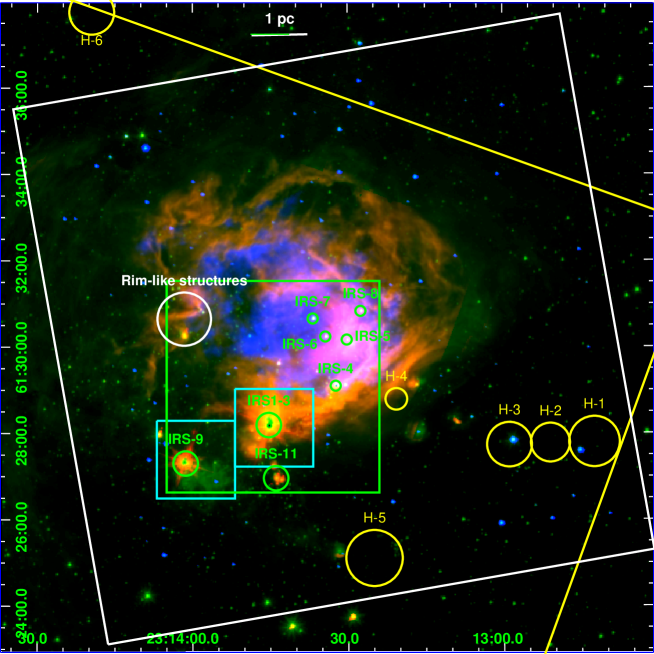
Figure 1: Color-composite image obtained by using the H$\alpha$ (blue), 3.6 $\mu$m (green), and 8.0 $\mu$m (red) images for an area of $\sim 15\times 15$ arcmin² around NGC 7538. White box represents the region covered in the optical survey. Region below the slightly horizontal yellow line and westward of slightly vertical yellow line represent the area covered in the $Chandra$ X-ray survey. The green and cyan boxes represent the areas covered by Ojha et al. (2004b) and Mallick et al. (2014) in their near-infrared (NIR) surveys, respectively. Positions of various IR sources (IRS 1-11), rim-like structures and $Herschel$-identified massive SFRs (H1 - H6) are also shown. The x-axis and y-axis are RA and Dec, respectively. in J2000 epoch.

The NGC 7538 region has been studied by Ojha et al. (2004b) by using NIR observations centered at IRS 1-3 (cf. Fig. 1), along with radio continuum observations at 1280 MHz. They have identified YSOs and classified them according to their evolutionary stages using NIR two-colour diagrams (TCDs) and generated the $K_{s}$-band luminosity function (KLF) to discuss the age sequence and mass spectrum of the YSOs in the region. They have discerned several substructures having different evolutionary stages. Balog et al. (2004) by using their NIR survey found that most of the red sources in this region are concentrated at the southern rim bounding the optical H II region and in the area around the IR sources IRS 1-3. Puga et al. (2010) have put an upper limit to the age of the central cluster as 2.2 Myr based on the lifetime of the most massive O3V star (60 M_⊙, IRS 6). Sandell & Sievers (2004), using their high spatial resolution submillimeter maps, found that the three major centers of star-forming activity (IRS 1-3, IRS 11, and IRS 9) in the NGC 7538 region are connected to each other through filamentary dust ridges. Recently, Mallick et al. (2014) have also observed in NIR the two comparatively smaller regions of NGC 7538 centered on IRS 1-3 and IRS 9 (cf. Fig. 1) to study the luminosity function (LF) and initial mass function (IMF) of these regions. They have complemented their deep NIR observations with X-ray, radio and molecular line observations to study the stellar population, ionized gas characteristics and dense molecular gas morphology in the region. Recently, Chavarría et al. (2014) have presented a homogeneous IR and molecular data to study the spatial distribution of YSOs and the properties of their clustering and correlation with the surrounding molecular cloud structures. They have compared these properties of this massive SFR with those of low-mass SFRs. However, they could not reach any concrete conclusion about the triggering mechanism due to the lack of the investigation of time causality between the expansion of the H II region and the age of the newly formed stars.

Most of the previous studies related to the star formation in this region are concentrated mainly on the IRS 1-11 region directly associated with NGC 7538. In the present work, we will revisit this region, but not only study a wider area but also make use of deep optical data of our own along with the multiwavelength archival data sets from various surveys ($Chandra$, Spitzer, 2MASS). Whereas the previous studies have neither derived the physical parameters (age/masses) of the individual YSOs nor checked for their association with the NGC 7538 region, we have done them and present a catalog of YSOs containing these information. For part of them spectral energy distribution (SED) fitting analyses have been applied. The spatial distribution of these YSOs, along with those of the mid-infrared (MIR) and radio emission, and the mass function (MF), will be used to constrain the star formation history in the region.

The rest of this paper is organized as follows: In Section 2, we describe the optical and archival data sets. In Section 3, we identify YSOs, catalog them according to their evolutionary stages, and derive their physical parameters. The X-ray spectral analysis of the YSOs is also explained in this section. All of these analyses are discussed in Section 4 and the conclusions are summarized in Section 5.

2 Observation and data reduction

2.1 Optical data

The CCD $UBV{(RI)}_{c}$ and $H\alpha$+continuum photometric data of the NGC 7538 region, centered at $\alpha_{J2000}$: 23^h13^m38^s, $\delta_{J2000}$: +61^∘31^′23^′′; $l=111.548^{\circ}$ and $b=0.832^{\circ}$, were acquired on 06, 07 November 2004 and 25 October 2005, respectively, by using the $2048\times 2048$ pixel² CCD camera mounted on the f/13 Cassegrain focus of the 104-cm Sampurnanand telescope of Aryabhatta Research Institute of Observational Sciences (ARIES), Nainital, India. In this set up, each pixel of the CCD corresponds to $0.37$ arcsec and the entire chip covers a field of $\sim 13\times 13$ arcmin² on the sky. To improve the signal to noise ratio (SNR), the observations were carried out in the binning mode of $2\times 2$ pixel. The read-out noise and gain of the CCD are 5.3 $e^{-}$ and 10 $e^{-}$/ADU respectively. The average FWHMs of the star images were $\sim 2$ arcsec. The broad-band $UBV{(RI)}_{c}$ observations of the NGC 7538 region were standardized by observing stars in the SA95 field (Landolt, 1992) centered on SA 112 ($\alpha_{J2000}$: 03^h53^m40^s, $\delta_{J2000}$: -00^∘00^′54^′′) on 06 November 2004. A reference field of $\sim 13\times 13$ arcmin² located about 10 arcmin away towards south-west of the NGC 7538 region was also observed to estimate the contamination due to foreground/background field stars on 30 November 2005 in $VI_{c}$. This reference field were standardized by using the common stars with the NGC 7538 region. The log of the observations is given in Table 1. In Fig. 1, we have shown the observed region (white box) on the colour-composite image of NGC 7538 obtained by combining the 3.6 $\mu$m (blue colour), H$\alpha$ (green colour) and 8.0 $\mu$m (red colour) images.

Table 1: Log of optical observations with the 104-cm Sampurnanand telescope, Nainital.

Date of observations/Filter	Exp. (sec)$\times$ No. of frames
	NGC 7538
06 November 2004
$U$	$300\times 4$
$B$	$180\times 4,60\times 3$
$V$	$60\times 4$
$R_{c}$	$30\times 4$
$I_{c}$	$30\times 4$
07 November 2004
$U$	$900\times 3$
$B$	$600\times 3$
$V$	$600\times 3$
$R_{c}$	$300\times 4$
$I_{c}$	$300\times 4$
25 October 2005
$H\alpha$	$900\times 2,300\times 3$
$Continuum$	$900\times 1,300\times 1$
	Reference field
30 November 2005
$V$	$600\times 3$
$I_{c}$	$300\times 3$

Figure 2: Differences between standard and transformed magnitudes and colours of standard stars plotted against the standard $V$ magnitude and $(B-V)$ colour.

Initial processing of the data frames was done by using the IRAF and ESO-MIDAS data reduction packages. Photometry of the cleaned frames was carried out by using DAOPHOT-II software (Stetson, 1987). The point spread function (PSF) was obtained for each frame by using several uncontaminated stars. Magnitudes obtained from different frames were averaged. When brighter stars were saturated on deep exposure frames, their magnitudes have been taken from short exposure frames. We used the DAOGROW program for construction of an aperture growth curve required for determining the difference between the aperture and PSF magnitudes.

Figure 3: DAOPHOT errors in magnitudes and colours as a function of $V$ magnitude.

Calibration of the instrumental magnitudes to the standard system was done by using the procedures outlined by Stetson (1992). The calibration equations derived by the least-squares linear regression are as follows:

$u=U+(7.178\pm 0.029)-(0.035\pm 0.039)(U-B)+(0.467\pm 0.046)X$,

$b=B+(4.771\pm 0.027)-(0.037\pm 0.028)(B-V)+(0.255\pm 0.025)X$,

$v=V+(4.274\pm 0.007)-(0.025\pm 0.005)(V-I_{c})+(0.143\pm 0.005)X$,

$r_{c}=R_{c}+(4.169\pm 0.005)-(0.028\pm 0.009)(V-R_{c})+(0.102\pm 0.003)X$,

$i_{c}=I_{c}+(4.611\pm 0.011)+(0.022\pm 0.008)(V-I_{c})+(0.072\pm 0.008)X$

where $U,B,V,R_{c}$ and $I_{c}$ are the standard magnitudes and $u,b,v,r_{c}$ and $i_{c}$ are the instrumental aperture magnitudes normalized for 1 second of exposure time and $X$ is the airmass. We have ignored the second-order colour correction terms as they are generally small in comparison to other errors present in the photometric data reduction. Fig. 2 shows the standardization residual, $\Delta$, between standard and transformed $V$ magnitudes and $(U-B),(B-V),(V-R_{c})$, and $(V-I_{c})$ colours of the standard stars as a function of $V$ magnitude and $(B-V)$ colour. As can be seen from the figure, the residuals are not showing any trends with colour or magnitude. The typical DAOPHOT errors in magnitude and colour as a function of $V$ magnitude, are shown in Fig. 3. It can be seen that, in the $V$ band, the errors become large ($\geq$0.1 mag) for stars fainter than $V\simeq 22$ mag, so the measurements beyond this magnitude are not reliable. In total 969 sources, with detection at least in the $V$ and $I_{c}$ bands and errors less than 0.1 mag, have been identified in this study.

2.2 Grism slitless spectroscopy

Slitless grism spectroscopy has also been carried out for the NGC 7538 region in search for H$\alpha$ emission stars. The observations were made with the Himalayan Faint Object Spectrograph Camera (HFOSC) on the 2-m Himalayan Chandra Telescope (HCT) of the Indian Astronomical Observatory (IAO), Hanle, India on 2004 September 21. A combination of a ‘wide H$\alpha$’ interference filter (6300-6740 Å) and grism 5 (5200-10300 Å) of HFOSC was used without slit. The central $2K\times 2K$ pixel of the $2K\times 4K$ CCD was used for data acquisition. The pixel size is 15 $\mu$m with an image scale of 0.297 arcsec pixel^-1. The resolution of the spectra is 870. We secured three spectroscopic frames of 5-min and 1-min exposure each with the grism in as well as three direct frames of 1-min exposure each with the grism out. The seeing size at the time of the observations was $\simeq$ 2 arcsec.

Table 2: $H\alpha$ emission stars identified by grism spectroscopy.

ID	$\alpha_{J2000}$	$\delta_{J2000}$	EW (H$\alpha$)
	(h:m:s)	(∘:′:′′)	(Å)
G1	23:13:16.66	+61:28:01.4	9.9
G2	23:13:32.75	+61:27:49.7	91.2
G3	23:13:56.36	+61:25:06.9	3.0
G4	23:14:06.64	+61:27:57.7	35.0
G5	23:14:13.04	+61:34:52.4	8.4
G6	23:14:13.38	+61:31:46.6	10.6

2.3 Archival data

2.3.1 $Chandra$ X-ray data

The NGC 7538 region has also been observed by $Chandra$ X-ray Observatory on 25 March, 2005 (cf. Fig. 1) centered at $\alpha_{J2000}$: 23^h13^m47.8^s, $\delta_{J2000}$: +61^∘28^′15.5^′′. The satellite roll angle (i.e. the orientation of the CCD array relative to north-south direction) during the observations was 19.2^∘. Exposures for 30 ks were obtained in the very faint data mode with a 3.2 s frame time by using the ACIS-I imaging array as the primary detector. ACIS-I consists of four front illuminated $1024\times 1024$ CCDs with a pixel size of 0.492 arcsec and a combined FOV of $\sim$17$\times$17 arcmin². The observed region of NGC 7538 by $Chandra$ is shown in Fig. 1. More detailed information on $Chandra$ and its instrumentation can be found in the $Chandra$ Proposer’s Guide. Tsujimoto et al. (2005) have used this data and presented a preliminary report indicating 180 X-ray sources in this region. 123 of them have 2MASS NIR counterparts. They have studied IR sources in this region and found that IRS 2, 4, 5, 6, 9 and 11 are bright in X-ray and have soft X-ray spectra similar to early type field stars. IRS 7 and 8 were identified as foreground stars due to absence of X-ray and, IRS 1 and IRS 2 were not detected probably due to high extinction.

Recently, Mallick et al. (2014) have reported 27 sources with NIR counterparts in the IRS 1-3 and IRS 9 regions (cf. Fig. 1).

In this study, X-ray data will be used to study the X-ray properties of the YSOs. We have used CIAO 4.8 data analysis software in combination with the $Chandra$ calibration database CALDB v.4.7.1 to reduce the X-ray data. The light curves from on-chip background regions were inspected for possible large background fluctuations that might have resulted from solar flares, however we did not find any such fluctuations. After filtering the data for the energy band 0.5 to 8.0 keV, the time integrated background was found to be 0.06 counts arcsec^-2. Source detection was then performed with the Palermo Wavelet Detection, PWDetect code (Damiani et al., 1997). It analyzes the data at different spatial scales, allowing the detection of both point-like and moderately extended sources, and efficiently resolving close pairs. The most important input parameter for this code is the detection threshold, which we estimated from the relationship between the background level and expected number of spurious detection due to Poisson noise (for detail, see Damiani et al., 1997). The background level was determined with the BACKGROUND command of XIMAGE. After filtering events in the energy band 0.5-8.0 keV, the ACIS-I observations comprise a total of about 56 k counts. This background level translates into a SNR threshold of 5.0 if we accept one spurious detection in the FOV, or into SNR 4.6 if we accept 10 spurious detections. The first choice results in detection of 158 sources, whereas the second one detects 193 sources. We decided to adopt the second criterion; however, we manually rejected 3 sources because they were detected either in the CCD gaps or twice. Finally, 190 X-ray point sources have been adopted for further analyses. The locations of these 190 X-ray point sources are shown in Fig. 4 overlaid on the $Chandra$ X-ray image.

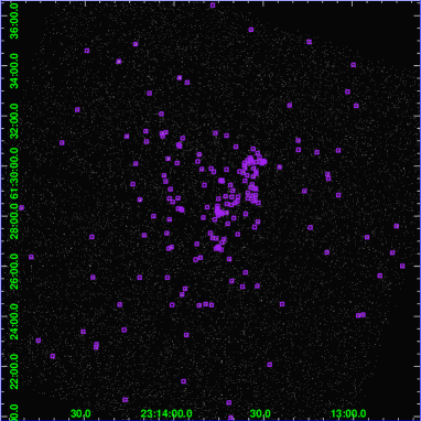
Figure 4: X-ray image obtained from the $Chandra$ observations. The identified point sources are shown by purple squares. The x-axis and y-axis are RA and Dec. in J2000 epoch.

2.3.2 Spitzer and 2MASS IR data

This region was observed by $Spitzer$ spacebased telescope on 14 August, 2006 (PI: Giovanni Fazio; program ID: 30784) with Infrared Array Camera (IRAC). These images have been mosaiced to create a $15\times 15$ arcmin² FOV (cf. Fig. 1) in all IRAC bands by using the MOPEX software provided by $Spitzer$ Science Center (SSC), containing the common area observed in the optical and X-ray wavelengths. These mosaiced images are used to make a color composite image (cf. Fig. 1) of this region.

Ojha et al. (2004b) have done NIR observations in a $5\times 5$ arcmin² FOV near IRS 1-3 (cf. Fig. 1) by using 2.2m University of Hawaii telescope. The NIR survey has 10$\sigma$ limiting magnitudes of 19.5, 18.4, and 17.3 in the $J$, $H$, and $K_{s}$ bands, respectively. Comparatively smaller regions ($1.8\times 1.8$ arcmin² FOV) centered on IRS 1-3 and IRS 9 (cf. Fig 1) were observed by using the 8.2m Subaru telescope by Mallick et al. (2014) in $J$, $H$, and $K$ bands. The 10$\sigma$ limiting magnitudes for these observations were $\sim$22, 21, and 20 in the $J$, $H$, and $K$ bands, respectively. Also, recently, Chavarría et al. (2014) have compiled $J$ and $K$ data (upto $K\sim 17.5$ mag) in a widest FOV of $20\times 20$ arcmin² in the NGC 7538 region using the 2.1m telescope at Kitt Peak National Observatory. These authors have published their YSOs catalog, which are merged together to form a combined catalog of YSOs (cf. Section 3.1.2) in the present study.

We have also used the 2MASS Point Source Catalog (PSC) (Cutri et al., 2003) for NIR (JHK_s) photometry in the NGC 7538 region. This catalog is reported to be 99$\%$ complete down to the limiting magnitudes of 15.8, 15.1 and 14.3 in the $J$, $H$ and $K_{s}$ band, respectively. We have selected only those sources which have NIR photometric accuracy $<$ 0.2 mag and detection in at least $H$ and $K_{s}$ bands.

3 Analysis and results

3.1 Identification of YSOs

YSOs are usually grouped into the evolutionary classes 0, I, II, and III, which represent in-falling protostars, evolved protostars, classical T-Tauri stars (CTTSs) and weak-line T-Tauri stars (WTTSs), respectively (cf. Feigelson & Montmerle, 1999a). Class 0 YSOs are so deeply buried inside the molecular clouds that they are not visible at optical or NIR wavelengths whereas Class I are characterized with the growth of an accretion disk surrounded by an envelope and are visible in IR and occasionally in optical if viewed in the pole-on direction (Nisini et al., 2005; White et al., 2007; Williams & Cieza, 2011). The CTTSs feature disks from which the material is accreted and line emission, e.g., in H$\alpha$, can be seen due to this accreting material. These disks can also be probed through their IR excess (over the normal stellar photospheres). WTTSs on the contrary have little or no disk material left and hence have no strong H$\alpha$ emission and IR excess. As the level of X-ray emission of pre-main sequence (PMS) stars are higher than that of MS stars (e.g., Feigelson & Montmerle, 1999b; Feigelson et al., 2002a; Favata & Micela, 2003; Güdel, 2004; Caramazza et al., 2012), X-ray observations provide a very efficient means of selecting WTTSs associated with the SFRs, which might be missed in the surveys based only on H$\alpha$ emission and/or IR excess emission. Below, we report identification of YSOs on the basis of their H$\alpha$, IR and/or X-ray emission.

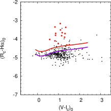
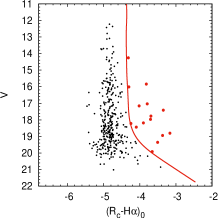
Figure 5: (Left-hand panel): $(R_{c}-H\alpha)_{0}$ index is shown as a function of $(V-I_{c})_{0}$ colour. The blue curve indicates the relation for MS stars as taken from Sung et al. (1997) and reddened for $A_{V}$= 2.3 mag (cf. Appendix A). The red curve yields the thresholds for H$\alpha$ emitter candidates (cf. Section 3.1.1). (Right-hand panel): $V$ versus $(R_{c}-H\alpha)_{0}$ CMD. The solid curve demarcates the H$\alpha$ emitter candidates from MS stars. The red dots represent selected H$\alpha$ emitting candidates.

3.1.1 H$\alpha$ emission

H$\alpha$ emission stars in a SFR are considered as PMS stars or candidates and the level of its strength (expressed by equivalent width ‘EW_Hα’) could be a direct indicator of their evolutionary stages. The conventional distinction between CTTS and WTTS is EW_Hα = 10Å  and it is greater for the former (cf. Herbig & Bell, 1988). The slitless grism frames were visually inspected to identify stars with H$\alpha$ enhancement. Then the EW_Hα of these stars has been estimated by using the APALL task of IRAF. EWs in pixels is converted into angstroms by multiplying 3.8 to it, as has been calculated for grism 5 having resolution R = 870 and assuming sampling of 2 pixels.

We have identified six H$\alpha$ emission stars spectroscopically and their position and EW_Hα are given in Table 2. Based on the value of EWs, three each were classified as Class II and Class III sources, respectively.

To identify H$\alpha$ emission stars we have also used narrow band H$\alpha$ photometry based on its excess emission. In the study of NGC 6383, Rauw et al. (2010) found that H$\alpha$ equivalent width of 10Åcorresponds to $(R_{c}-H\alpha)$ index of 0.24 $\pm$ 0.04 mag above the MS relation introduced by Sung et al. (1997). In the present study, we have used this condition to identify H$\alpha$ emission stars and classified them as Class II sources. Since our H$\alpha$ photometry is not calibrated, in order to compare this H$\alpha$ magnitude to that of Sung et al. (1997), we estimated the zero point by comparing visually the observed $(R_{c}-H\alpha)$ and dereddened $(V-I_{c})$ with the $(R_{c}-H\alpha)_{0}$ versus $(V-I_{c})_{0}$ relation of emission-free MS stars as determined by Sung et al. (1997) for the NGC 2264 region. We have to subtract 3.85 mag from the observed values to obtain $(R_{c}-H\alpha)$ index in the Sung et al. (1997) system. The $(V-I_{c})$ colour is dereddened by the minimum extinction value derived in Appendix A (i.e., $E(B-V)_{min}$ = 0.75 mag and $R_{V}$ = 2.82). In the left-hand panel of Fig. 5, we have plotted the $(R_{c}-H\alpha)_{0}$ versus $(V-I_{c})_{0}$ distribution of all the stars along with the MS relation (blue curve) given by Sung et al. (1997). All the sources above the red curve (0.24 mag above the MS relation, cf., Sung et al., 1997) are assumed as H$\alpha$ excess emission sources of Class II evolutionary stage. Since there is a large scatter in the distribution in Fig. 5; left-hand panel, there may be some false identifications of H$\alpha$ emitters. To minimize false detections, we have introduced another selection criterion using the $V$ versus $(R_{c}-H\alpha)_{0}$ CMD (cf. Fig. 5; right-hand panel). We define an envelope which contains MS stars keeping in mind its broadening at faint magnitudes due to large photometric errors, possible presence of binaries, field stars etc. (Phelps & Janes, 1994). The stars which are having values of $(R_{c}-H\alpha)_{0}-\sigma_{(R_{c}-H\alpha)_{0}}$ larger than that of the envelope of the MS can be safely assumed as probable H$\alpha$ emitters (Kumar et al., 2014). Our final criterion for photometrically selected H$\alpha$ emitters is to satisfy both of the above conditions. 15 sources (red dots in Fig. 5) were identified as H$\alpha$ emitting YSOs and were categorized as Class II YSOs. None of them were identified through grism spectroscopy.

In total 21 stars were classified as YSOs (3 as Class III and 18 as Class II) on the basis of H$\alpha$ spectroscopy and photometry.

3.1.2 IR emission

Recently, Chavarría et al. (2014) have identified 562 YSOs in a $15\times 15$ arcmin² FOV of the NGC 7538 region on the basis of NIR/MIR excess emission. They classified 234 YSOs which have detections in all four IRAC bands on the basis of the value of the slopes ‘$\alpha_{IRAC}$’ of their SEDs. We further used [[3.6] - [4.5]]₀ versus [[$K$] - [3.6]]₀ TCD (for details see, Gutermuth et al., 2009) for the classification of remaining YSOs. YSOs having $[J-H]$ color $\geq 0.6$ mag and lying above the CTTS locus or its extension are traced back to CTTS locus or its extension to get their intrinsic colors. For YSOs that lack $J$ band photometry, baseline colors in the $[H-K]$ versus [[3.6] - [4.5]] color-color space YSO locus, as measured by Gutermuth et al. (2005) is used to get their intrinsic colors. 43 Class I and 108 Class II sources were classified by using their location in the above mentioned TCD and are shown as yellow circles and red dots, respectively in Fig. 6. For those YSOs which are not detected in the IRAC bands but have NIR $(JHK)$ detections and have $(J-H)>0.6$ mag (13 sources), we have used the classical NIR TCDs (cf. Ojha et al., 2004b; Sharma et al., 2012) for their classifications. Finally, out of 562 YSOs, 239 (234 IRAC four band sources plus 5 MIPS sources) were classified by Chavarría et al. (2014) and 164 are classified in this study. Remaining 159 YSOs could not be classified as either they have no IRAC detections and $(J-H)<0.6$ mag or they do not fall at the location of Class I/II YSOs in IRAC [[3.6] - [4.5]]₀ versus [[$K$] - [3.6]]₀ TCD.

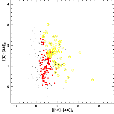
Figure 6: ${[[K]-[3.6]]}_{0}$ vs. ${[[3.6]-[4.5]]}_{0}$ TCD for those YSOs identified by Chavarría et al. (2014) that lack detection at either 5.8 $\mu$m or 8.0 $\mu$m, but have NIR detection in the $K$ band (black dots). The YSOs classified as Class I and Class II, based on the colour criteria by Gutermuth et al. (2009), are shown by using yellow circles and red dots, respectively.

Ojha et al. (2004b) have studied the NGC 7538 region and identified and classified 286 YSOs (18 Class I and 268 Class II YSOs) based on their excess emission in IR using their location in the NIR TCD (e.g. Fig. 7). The solid and thick black dashed curves in Fig. 7 represent the un-reddened MS and giant branch (Bessell & Brett, 1988), respectively. The dotted blue line indicates the locus of un-reddened CTTSs (Meyer et al., 1997). The parallel dashed red lines are the reddening lines drawn from the tip (spectral type M4) of the giant branch (“upper reddening line"), from the base (spectral type A0) of the MS branch (“middle reddening line") and from the tip of the intrinsic CTTS line (“lower reddening line"). The extinction ratios $A_{J}/A_{V}=0.265,A_{H}/A_{V}=0.155$ and $A_{K}/A_{V}=0.090$ have been taken from Cohen et al. (1981). These extinction ratios are for the normal Galactic medium (i.e., $R_{V}$= 3.1), since for $\lambda>\lambda_{I}$ the reddening law can be taken as a universal quantity (Cardelli et al., 1989; He et al., 1995). The sources can be classified according to the three regions in this diagram (cf. Ojha et al., 2004a). ‘F’ sources are located between the upper and middle reddening lines and are considered to be either field stars (MS stars, giants) or Class III sources and Class II sources with small NIR excess. ‘T’ sources are located between the middle and lower reddening lines. These sources are considered to be mostly CTTSs (or Class II objects) with large NIR excess. There may be an overlap of Herbig Ae/Be stars in the ‘T’ region (Hillenbrand et al., 1992). ‘P’ sources are those located in the region red-ward of the lower reddening line and are most likely Class I objects (protostellar-like objects; Ojha et al. (2004a)). Most recently, Mallick et al. (2014) also identified and classified 168 YSOs (24 Class I and 144 Class II) similarly in the IRS 1-3 region. We combined these two NIR data sets with a match radius of 1 arcsec and cataloged 408 YSOs (40 Class I and 368 Class II; 46 were in both catalogs). After combining this catalog with that of Chavarría et al. (2014, 562 YSOs) with the same match radius of 1 arcsec, we compiled altogether 890 YSOs (80 YSOs were in both catalogs) in the selected region of NGC 7538. 169, 569 and 3 are Class I, Class II and Class III objects, respectively. The details are given in Table 3.

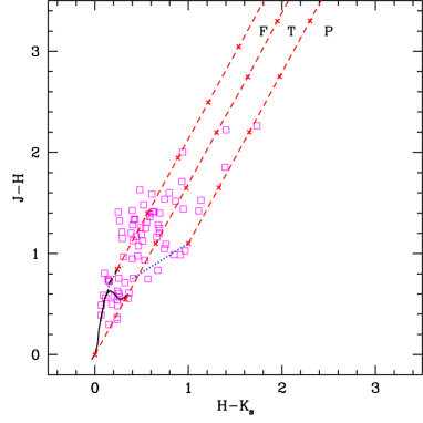
Figure 7: NIR TCD for the sources having X-ray counterparts (purple squares) in the NGC 7538 region. The continuous and thick black dashed curves represent the dereddened MS and giant branches (Bessell & Brett, 1988), respectively. The dotted blue line indicates the locus of dereddened CTTSs (Meyer et al., 1997). The parallel red dashed lines are the reddening lines drawn from the tip (spectral type M4) of the giant branch (left reddening line), from the base (spectral type A0) of the MS branch (middle reddening line) and from the tip of the intrinsic CTTS line (right reddening line). The crosses on the reddening lines show an increment of $A_{V}$ = 5 mag.

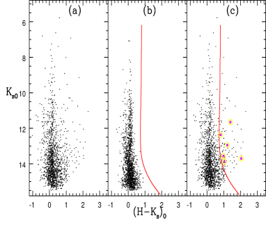
Figure 8: $K_{s}{{}_{0}}/(H-K_{s}){{}_{0}}$ CMD for (a) stars in the NGC 7538 region, (b) stars in the reference field and (c) identified X-ray emitting IR excess stars (purple squares inside yellow circles). The red thick line demarcates the X-ray emitting IR excess stars from MS stars.

3.1.3 X-ray emission

The sample of the YSOs selected on the basis of IR excess may be incomplete because the circumstellar-disks in young stars may disappear on time-scales of just a few Myr (see Briceño et al., 2007). Recent studies of a few SFRs reveal that disk fraction decreases with age of the region, e.g., Sh 2-311: 35% disk fraction, age=4 Myr, distance = 5 kpc (Yadav et al., 2016); NGC 2282: 58% disk fraction, age= 2-5 Myr, distance=1.65 kpc (Dutta et al., 2015); W3-AFGL333: 50-60% disk fraction, age=2 Myr, distance=2 kpc (Jose et al., 2016). Since the average age of the YSOs in NGC 7538 region is 1.4 Myr (cf. Section 4.1), we can expect less than 40% of YSOs do not show excess emission in NIR/MIR (Haisch et al., 2001; Hernández et al., 2008).

Since X-ray detection method is sensitive also to young stars that have already dispersed their circumstellar disks (Preibisch et al., 2011), we have paid attention to X-ray emitting stars and classified them according to their evolutionary stages using the classical NIR TCDs (Jose et al., 2008; Pandey et al., 2008; Sharma et al., 2012; Kumar et al., 2014).

In Fig. 7, we have plotted the NIR TCD for the X-ray counterparts. Since none of the previous studies on the NGC 7538 region (cf. Ojha et al., 2004b; Mallick et al., 2014; Chavarría et al., 2014) have published their deep photometric catalogs online, we have used 2MASS data to find the NIR counterparts of the X-ray sources. The Chandra on-axis point-spread function (PSF) is $0.5^{\prime\prime}$ and it degrades at large off-axis angles (see e.g. Getman et al., 2005; Broos et al., 2010). So we used an optimal matching radius of 1 arcsec to determine the 2MASS NIR counterparts of the X-ray sources. This size of the matching radius is well established in other studies as well (see e.g. Feigelson et al., 2002a; Wang et al., 2007). Ninety of the X-ray emitting sources have 2MASS NIR counterparts falling in the our selected region ($15\times 15$ arcmin² FOV) of NGC 7538. All the 2MASS magnitudes and colours have been converted into the California Institute of Technology (CIT) system. All the curves and lines are also in the CIT system. The sources falling in the ‘F’ region and above the extension of the intrinsic CTTS locus as well as the sources having $(J-H)\geq 0.6$ and lying to the left of the upper reddening line are assigned as WTTSs/Class III sources (45 sources) (see, e.g., Jose et al., 2008; Pandey et al., 2008; Sharma et al., 2012; Kumar et al., 2014). The X-ray counterparts falling in the ‘T’ (12 sources) and ‘P’ (1 sources) regions are classified as Class II and Class I sources, respectively.

Sixteen X-ray sources do not have $J$ band data. The classification of these sources was done by comparing the dereddened $K_{s}{{}_{0}}/(H-K_{s}){{}_{0}}$ CMD of the studied region with that of the reference field, having the equal area (cf. Fig. 8). This scheme has been explained in detail by Kumar et al. (2014). The amounts of reddening and extinction were estimated on the extinction map obtained by using the NIR TCD. Briefly, the stars having $(J-H)$ colour $\geq 0.6$ mag and lying above the CTTS locus or its extension were traced back to the CTTS locus or its extension to get their amounts of reddening. Once we have the amount of reddening for individual stars, we can generate extinction maps for the target and field regions. The extinction maps were then used to deredden the remaining stars. The red solid curve in Fig. 8 represents the outer boundary of the field star distribution in the CMD taking into account the scatter due to photometric errors and variations in the $A_{V}$ values (see for details, Kumar et al., 2014). All the stars having a colour ‘$(H-K)_{0}-\sigma_{(H-K)_{0}}$’ larger than the $red$ cut-off curve in the studied region, are believed to have excess emission in the $K_{s}$ band and can be presumed as Class I YSOs (see also Ojha et al., 2004b; Mallick et al., 2012; Kumar et al., 2014). We have classified six sources without $J$ band detections as Class I on the basis of the above criterion.

In total 64 sources with X-ray emission were classified as YSOs (45 as Class III, 12 as Class II and 7 as Class I) on the basis of their positions in the NIR TCD/CMD.

3.1.4 The YSOs sample

We have cross identified the YSOs detected in the present survey based on H$\alpha$ (21 sources, cf. 3.1.1) and X-ray emission (64 sources, cf 3.1.3) with those which were detected on the basis of excess IR emission and are available in the literature (890 sources, cf. Section 3.1.2 and Table 3, Ojha et al., 2004b; Mallick et al., 2014; Chavarría et al., 2014), using a search radius of 1 arcsec. We found 6 H$\alpha$ and 26 X-ray emitting sources are also showing excess IR emission, thus we confirmed their identification. The remaining 53 sources (cf. Table 4) are new additions and have been added to make a catalog of altogether 943 YSOs in the 15$\times$15 arcmin² field around NGC 7538. Optical counterparts for 74 of these YSOs were also identified by using a search radius of 1 arcsec. The position, magnitude, colour and classification of these YSOs are given in Table 5.

Since the aim of this work is to study the star formation activities in the NGC 7538 region, the information regarding individual properties of the YSOs is vital, which are derived by using the SED fitting analysis (cf. Section 3.2.1). The SEDs of YSOs can be generated by using the multiwavelength data (i.e. optical to MIR) under the condition that a minimum of 5 data points should be available. Out of 943 YSOs, 463 satisfy this criterion and therefore are used in the further analysis. The evolutionary classes of most of these YSOs were defined on the basis of available data sets. First they were classified on the basis of $\alpha_{IRAC}$ (cf. Chavarría et al., 2014). Those which do not have $\alpha_{IRAC}$, were then classified on the basis of MIR+NIR TCD. And if IRAC data are not available, then the NIR TCD classification scheme was used (cf. Section 3.1.2). Finally, the newly identified YSOs on the basis of their X-ray and H$\alpha$ emission (cf. Section 3.1.1 and Section 3.1.3) were classified based on their IR excess properties and EWs of H$\alpha$ line, respectively.

3.1.5 Source contamination and the completeness of the YSOs sample

We have a sample of 419 YSOs for which SEDs can be generated and are associated with the NGC 7538 SFR. Our candidate YSOs may be contaminated by IR excess sources such as star forming galaxies, broad-line active galactic nuclei, unresolved shock emission knots, objects that suffer from polycyclic aromatic hydrocarbon (PAH) emissions etc., that mimic the colours of YSOs. Since we are observing through the Galactic plane, contamination due to galaxies should be negligible (Massi et al., 2015). In order to have a statistical estimate of possible galaxy contamination in our YSOs sample, we used the Spitzer Wide-area Infrared Extragalactic (SWIRE) catalog obtained from the observations of the ELAIS N1 field (Rowan-Robinson et al., 2013). SWIRE is a survey of the extragalactic field using the Spitzer-IRAC and MIPS bands and can be used to predict the number of galaxies in a sample of YSOs (Evans et al., 2009). The SWIRE catalog is resampled for the spatial extent as well as the sensitivity limits of the photometric data in the NGC 7538 region and is also corrected by the average extinction (i.e. $A_{V}$ = 11 mag, cf. Section 4.1). 17 sources in the SWIRE catalog could satisfy these criteria. Similarly, out of the 397 YSOs having IRAC photometry, 7 can be approximately categorized as obscured AGB stars as they have very bright MIR flux, i.e., [4.5]$\leq$7.8 mag (cf. Robitaille et al., 2008). Therefore, the contribution of various contaminants in our YSO sample should be $\sim$6%, which is a small fraction of the total number of YSOs. We also applied the colour/magnitude criteria by Gutermuth et al. (2009) to the YSOs classified by Chavarría et al. (2014) on the basis of their IRAC SEDs, and $\sim$28% of them are matched with the colours of PAH contaminated apertures, shock emissions, PAH emitting galaxies and AGNs. Recently, Jose et al. (2016) have also checked the same scheme applied to their sample of YSOs in the W3-AFGL333 region and found that $\sim$38% of Class I sources and $\sim$15% of Class II sources in their sample turned out to be contaminants. However, using statistical approach as used by us, they have found only $<$5% contaminants in their sample of YSOs. Several studies (e.g., Koenig et al., 2008; Rivera-Ingraham et al., 2011; Willis et al., 2013) have noticed that the use of the Gutermuth et al. (2009) criteria for a region at $\sim$2 kpc would likely provide an overestimation of the contaminations.

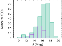
Figure 9: Histogram (green) showing the distribution of the number of YSOs in different $J$ magnitude (left-hand panel) and the corresponding mass limit of the YSOs (right-hand panel). The blue histogram represents the sample of X-ray emitting YSOs (64) having 2MASS detections.

For the above mentioned sample of YSOs having data taken from various surveys, knowledge of its completeness in terms of mass is necessary, but we cannot perform the $ADDSTAR$ routine to derive it. Therefore, we have instead drawn histograms for the numbers of YSOs in different magnitude bins and checked for their peaks. This peak will roughly represent the completeness limit of the data in terms of magnitude (Jose et al., 2013; Willis et al., 2013; Jose et al., 2016; Sharma et al., 2016). Once we know this, the corresponding mass is taken as that of the lowest mass YSO. For example, in Fig. 9 we show the distribution of the numbers of YSOs in different $J$ magnitudes and the corresponding mass limit of the YSOs. The peak of this histogram is in between 17-18 mag and for this magnitude bin the corresponding mass is 0.5 M_⊙. In this way we found that our data are complete down to 0.5, 0.8, 0.8, 0.8 and 0.6 M_⊙ in the $J$, $H$, $K_{s}$, 3.6 $\mu$m and 4.8 $\mu$m bands, respectively. Since the sources undetected at 5.8 $\mu$m and 8.0 $\mu$m were classified on the basis of the 3.6 $\mu$m, 4.8 $\mu$m, $H$ and $K_{s}$ band photometry, the completeness limit for them is not included here. The mass completeness for the YSOs having X-ray and H$\alpha$ emission will depend on the completeness limit of the photometric data from which they were identified. The completeness limit for the X-ray emitting YSOs (64) comes out to be 0.8 M_⊙ as inferred from the peak of the blue histogram in Fig. 9. For the H$\alpha$ emitting sources, their completeness can be approximated as 0.8 M_⊙, which is equivalent to that of the optical data. To conclude, we have taken the highest of these, i.e., 0.8 M_⊙, as the completeness limit for the detection of the current YSO sample.

Table 3: A sample table containing information for 890 cataloged YSOs by Ojha et al. (2004b), Chavarría et al. (2014) and Mallick et al. (2014) in the NGC 7538 region. The complete table is available in an electronic form only.

ID∗	$\alpha_{(2000)}$	$\delta_{(2000)}$	Classa	Classb	Classc	Classd
	(h:m:s)	(∘:′:′′)
$C_{2361}$	23:12:34.40	+61:27:11.3	II	-	-	-
$C_{2362}$	23:12:37.42	+61:36:16.2	-	-	-	-
$C_{2363}$	23:12:40.88	+61:24:56.5	II	-	-	-
$C_{2364}$	23:12:40.88	+61:31:38.8	II	-	-	-
$C_{2365}$	23:12:41.18	+61:28:02.1	II	-	-	-

^∗: O, C and M are YSOs cataloged in Ojha et al. (2004b), Chavarría et al. (2014) and Mallick et al. (2014), respectively.
^a: Classification by Chavarría et al. (2014) based on IRAC SED slope.
^b: Classification by IRAC TCDs.
^c: Classification by Ojha et al. (2004b) and Mallick et al. (2014) through NIR TCDs.
^d: Classification by H$\alpha$ and X-ray emission (i.e., I/II/III(Comment), if Comment=7: H$\alpha$ emission star (spectroscopy), Comment=8: H$\alpha$ emission star (photometry), Comment=9: X-ray emitting star.

Table 4: A sample table containing information for 53 newly identified YSOs. The $J$, $H$ and $K_{s}$ magnitudes and their errors are from the 2MASS PSC. The complete table is available in an electronic form only.

ID	$\alpha_{(2000)}$	$\delta_{(2000)}$	$J\pm\sigma$	$H\pm\sigma$	$K_{s}\pm\sigma$	Classd
	(h:m:s)	(∘:′:′′)	(mag)	(mag)	(mag)
$S_{1}$	23:13:49.12	+61:30:15.4	$11.966\pm 0.024$	$11.120\pm 0.030$	$10.783\pm 0.019$	II(8)
$S_{2}$	23:13:29.47	+61:30:38.9	$12.447\pm 0.034$	$11.945\pm 0.039$	$11.649\pm 0.039$	II(8)
$S_{3}$	23:13:56.29	+61:25:07.3	$13.455\pm 0.031$	$12.843\pm 0.035$	$12.553\pm 0.032$	III(7)
$S_{4}$	23:14:15.91	+61:31:12.1	$13.608\pm 0.027$	$12.843\pm 0.028$	$12.666\pm 0.023$	III(9)
$S_{5}$	23:13:31.96	+61:27:47.3	$13.697\pm 0.030$	$12.223\pm 0.032$	$11.495\pm 0.019$	III(9)

^d: Classification by H$\alpha$ and X-ray emission (i.e., I/II/III(Comment), if Comment=7: H$\alpha$ emission star (spectroscopy), Comment=8: H$\alpha$ emission star (photometry), Comment=9: X-ray emitting star.

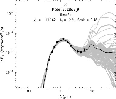
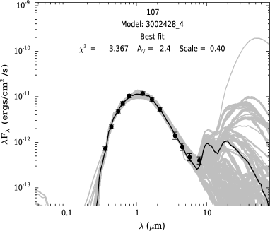
Figure 10: Sample SEDs for Class I (left-hand panel) and Class II (right-hand panel) sources created by the SED fitting tools of Robitaille et al. (2007). The black curve shows the best fit and the gray curves show the subsequent well fits. The filled circles with error bars denote the input flux values.

3.2 YSOs parameters

3.2.1 From spectral energy distribution analysis

We constructed SEDs of the YSOs using the grid models and fitting tools of Robitaille et al. (2006, 2007) for characterizing and understanding their nature. The models were computed by using a Monte-Carlo based 20000 2-D radiation transfer calculations from Whitney et al. (2003b, a, 2004) and by adopting several combinations of a central star, a disk, an in-falling envelope, and a bipolar cavity in a reasonably large parameter space and with 10 viewing angles (inclinations). The SED fitting tools provide the evolutionary stage and physical parameters such as mass, age, disk mass, disk accretion rate and stellar temperature of YSOs and hence are an ideal tool to study the evolutionary status of YSOs.

We constructed the SEDs of 463 YSOs using the multiwavelength data (optical to MIR wavelengths, i.e. 0.37, 0.44, 0.55, 0.65, 0.80, 1.2, 1.6, 2.2, 3.6, 4.5, 5.8 and 8.0 $\mu m$) and with a condition that a minimum of 5 data points should be available (cf. Section 3.1.4). The SED fitting tool fits each of the models to the data allowing the distance and extinction as free parameters. The distance of the NGC 7538 region is taken as 2.65${}^{+0.12}_{-0.11}$ kpc (cf. Appendix A), but the input value ranges to the fitting tool is given with three times the error of the adopted distance, i.e., 2.65-0.12$\times$3 to 2.65+0.12$\times$3 = 2.3 to 3.0 kpc. Since, this region is highly nebulous and Ojha et al. (2004b, Fig. 6) detected YSOs up to $A_{V}$ = 25 mag, we varied $A_{V}$ in a broader range (i.e., from 0 to 30 mag) with three times the errors associated with the foreground $A_{V}$ value ($\pm$2 mag, cf. Appendix A) and keeping in mind the nebulosity associated with this SFR (see also, Samal et al., 2012; Jose et al., 2013; Panwar et al., 2014).

We further set photometric uncertainties of 10% for optical and 20% for both NIR and MIR data. These values are adopted instead of the formal errors in the catalog in order to fit without any possible bias caused by underestimating the flux uncertainties. We obtained the physical parameters of the YSOs using the relative probability distribution for the stages of all the ‘well-fit’ models. The well-fit models for each source are defined by

$\chi^{2}-\chi^{2}_{min}\leq 2N_{data}$

where $\chi^{2}_{min}$ is the goodness-of-fit parameter for the best-fit model and $N_{data}$ is the number of input data points. In Fig. 10, we show example SEDs of Class I and Class II sources, where the solid black curves represent the best-fit and the gray curves are the subsequent well-fits. As can be seen, the SED of the Class I source rises substantially in the MIR in comparison to that of the Class II source due to its optically thick disk. The sheer number of gray curves in the SED indicates how difficult it was to select a single best-fitting model to these data, which is not surprising given that there are no anchors at long wavelengths. Here it is worthwhile to take note that the Class I source shown in Fig. 10 is optically detected, which is not usual, but there are also several other cases where such Class I sources are not detected optically, e.g., Pandey et al. (2013, NGC 1931), Jose et al. (2013, Sh 2-252), Chauhan et al. (2011, W5-East), Ojha et al. (2011, Sh 2-255-257) and Yadav et al. (2016, Sh-2 311). In the present study, five Class I sources have optical detections. Optical detection of Class I sources can be attributed to their viewing angle (Nisini et al., 2005; White et al., 2007; Williams & Cieza, 2011). Also, some Class I and Class II sources can exhibit similar SEDs in the $Spitzer$ bands (Hartmann et al., 2005; Williams & Cieza, 2011; Robitaille et al., 2006). As an example, the models of Whitney et al. (2003a) show that mid-latitude ($\sim 40^{\circ}$)-viewed Class I stars have optical and NIR/MIR characteristics similar to those of more edge-on disk ($\sim 75^{\circ}$) Class II stars. The effects of the edge-on disk orientation are most severe for evolutionary diagnostics determined in the NIR/MIR such as the 2-25 $\mu$m spectral index (White et al., 2007). The definitive identification of Class I sources requires other observations that better constrain the presence of an envelope, such as MIR spectroscopy, far-IR and millimeter photometry, and high-resolution images (Luhman et al., 2010).

From the well-fit models for each source derived from the SED fitting tool, we calculated the $\chi^{2}$ weighted model parameters such as the $A_{V}$, distance, stellar mass and stellar age of each YSO and they are given in Table 6 along with their adopted evolutionary classes (cf. Section 3.1.4). The error in each parameter is calculated from the standard deviation of all well-fit parameters.

Table 5: A sample table containing information for 74 optically identified YSOs. The age and mass of the YSOs are derived from the optical CMD. IDs are the same as in Table 3 and Table 4. The complete table is available in an electronic form only.

ID	$V\pm\sigma$	$(U-B)\pm\sigma$	$(B-V)\pm\sigma$	$(V-R_{c})\pm\sigma$	$(V-I_{c})\pm\sigma$	Age$\pm\sigma$	Mass$\pm\sigma$
	(mag)	(mag)	(mag)	(mag)	(mag)	(Myr)	(M⊙)
$C_{2833}$	$12.369\pm 0.004$	$-0.047\pm 0.005$	$0.611\pm 0.005$	$0.401\pm 0.007$	$0.806\pm 0.008$	$0.4\pm 0.1$	$5.8\pm 0.1$
$C_{2864}$	$13.903\pm 0.005$	$0.676\pm 0.007$	$0.970\pm 0.006$	$0.576\pm 0.011$	$1.077\pm 0.009$	$1.2\pm 0.1$	$3.9\pm 0.3$
$C_{2523}$	$14.259\pm 0.007$	$0.081\pm 0.006$	$1.402\pm 0.008$	$1.050\pm 0.012$	$2.251\pm 0.013$	$0.1\pm 0.1$	$5.4\pm 0.1$
$C_{2411}$	$14.360\pm 0.006$	$0.016\pm 0.006$	$0.742\pm 0.006$	$0.460\pm 0.009$	$0.950\pm 0.009$	$2.5\pm 1.9$	$4.9\pm 0.3$

Table 6: A sample table containing stellar parameters of selected 419 YSOs derived by using the SED fitting analysis. IDs are the same as in Table 3 and Table 4. The complete table is available in an electronic form only.

ID	$N_{data}$	Class	$\chi^{2}_{min}$	Distance$\pm\sigma$	$A_{V}$$\pm\sigma$	Age$\pm\sigma$	Mass$\pm\sigma$
				(kpc)	(mag)	(Myr)	($M_{\odot}$)
$C_{2361}$	6	II	1.7	$2.5\pm 0.2$	$19.8\pm 3.7$	$0.8\pm 0.9$	$1.7\pm 1.0$
$C_{2363}$	6	II	3.1	$2.6\pm 0.3$	$18.0\pm 2.6$	$1.2\pm 1.7$	$1.1\pm 0.8$
$C_{2364}$	7	II	0.7	$2.6\pm 0.3$	$4.4\pm 1.8$	$1.5\pm 1.5$	$1.2\pm 0.7$
$C_{2365}$	6	II	0.6	$2.6\pm 0.3$	$21.2\pm 3.6$	$1.0\pm 1.4$	$1.5\pm 0.9$

The evolutionary class of the YSOs are from Table 3 and Table 4 (cf. Section 3.1.4).

3.2.2 From optical colour-magnitude diagram

By comparing the positions of YSOs in the optical CMD with theoretical isochrones, we can determine their age and mass. In Fig. 11, the $V/(V-I_{c})$ CMD has been plotted for all the sources in the NGC 7538 region along with optically detected 74 YSOs. The post-main-sequence isochrone for 2 Myr calculated by Marigo et al. (2008) (thick black curve) along with the PMS isochrones of 0.1,0.5,1,2,5,10 Myr (red dashed curves) and evolutionary tracks of different masses (red curves) by Siess et al. (2000) are also shown. These isochrones are corrected for the distance (2.65${}^{+0.12}_{-0.11}$ kpc, cf. Appendix A) and the foreground reddening ($E(B-V)_{min}=0.75\pm 0.2$ mag, cf. Appendix A) of NGC 7538 by using the reddening law $R_{V}$=2.82 (cf. Appendix B). Here, it is highly likely that not all the YSOs are situated on the surface of the associated cloud but embedded in it where the reddening law is anomalous ($R_{V}$=3.85, cf. Appendix B). Change of the reddening law can affect the derivation of the physical parameters of the YSOs. Therefore, we checked the change in the position of a YSO in the dereddened optical CMD, corrected for the extinction $A_{V}$= 3 mag (i.e. the average extinction value of the optically detected YSOs, cf. Section 3.2.1, Table 6) by applying different $R_{V}$ values. After removing the foreground contribution, the intra-cluster extinction in $V$ and $(V-I_{c})$ will be 0.9 mag and 0.34 mag, respectively for $R_{V}$=3.85 and, 0.7 mag and 0.28 mag, respectively for $R_{V}$ = 2.82. Therefore, the change in reddening law will have a marginal effect to the derived physical parameters. But the amount of intra-cluster reddening can affect the derivation of ages/masses of YSOs, if not corrected individually. As we can see from Fig. 11, the reddening vector is almost parallel to the isochrones, but nearly perpendicular to the evolutionary tracks for various masses, this effect will be nominal in deriving the ages, but can be substantial in the mass estimation.

The age and mass of the YSOs have been derived from the optical CMD (cf. Fig. 11) by applying the following procedure. We created an error box around each observed data point using the errors associated with photometry as well as errors associated with the estimation of reddening and distance as given in previous paragraph. Five hundred random data points were generated by using Monte-Carlo simulations in this box. The age and mass of each generated point were estimated from the nearest passing isochrone and evolutionary track by Siess et al. (2000). For accuracy, the isochrones and evolutionary tracks were used in a bin size of 0.1 Myr and were interpolated by 2000 points. At the end we have taken their mean and standard deviation as the final derived values and errors and are given in Table 5.

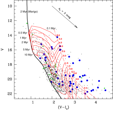
Figure 11: $V/(V-I_{c})$ CMD for all the optically detected sources in the NGC 7538 region. Blue dots are identified YSOs and green circles are the sources categorized as non-members of the region (cf. Section 4.1 for detail). The isochrone for 2 Myr by Marigo et al. (2008) (thick black curve) along with the PMS isochrones of 0.1,0.5,1,2,5,10 Myr (red dashed curves) and the evolutionary tracks of different masses (red curves) by Siess et al. (2000) are also shown. All the isochrones and evolutionary tracks are corrected for the distance of 2.65 kpc and reddening $E(B-V)=0.75$ mag.

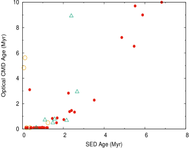
Figure 12: Comparison of the age estimates obtained from the CMD analysis with those from the SED fitting. Yellow open circles, red filled circles and green open triangles represent Class I, Class II and Class III sources, respectively.

In Fig. 12, we have compared the age estimates obtained from the CMD and the SED fitting. The distribution indicates in general a reasonable agreement between them with a large scatter. We have calculated the linear Pearson correlation coefficient (r=0.71) for this distribution and found that the probability of having no correlation is negligible (i.e., 10^-6). The scatter in Fig. 12 may be due to the difference in reddening/extinction corrections to the magnitudes/colours of the YSOs in these two techniques. In the optical CMD, we have used a fixed foreground reddening value for all the YSOs, while in the SED fitting, $A_{V}$ was given as a free parameter in a broad range to deredden the individual YSOs. Therefore, by the CMDs the very young YSOs which tend to be deeply embedded in the cloud can be assigned lower ages than their actual ones. ここ

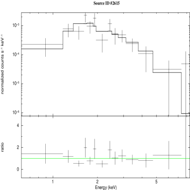
Figure 13: An example X-ray spectrum of a YSO (source ID 2615) fitted by the spectral model phabs $\times$ Apec.

3.3 X-ray spectral analysis

Present data contains 190 X-ray emitting sources, of which 91 are classified as YSOs, either on the basis of their location on the NIR TCD/CMD (64, cf. Section 3.1.3), or having their counterpart in already published list of YSOs (27, cf. Section 3.1.2). For X-ray spectral analysis, we have selected 21 of them, having more than 35 counts (SNR $>$ 5) in the energy band 0.2-8.0 keV to ensure a minimum quality of spectral fits. The spectra of these sources and the background were extracted by using the $specextract$ task. The radii of the extracted regions of the sources varied between 5 arcsec and 15 arcsec depending on the position of the source detected by the $PWDetect$ task (see Section 2.3.1) on the detector as well as on its angular separation with respect to the neighboring X-ray sources. For each source, the background spectrum was obtained from multiple source-free regions chosen according to the source location on the same CCD. The spectra were binned to have a minimum of 5 counts per spectral bin by using $grppha$ task included in ftools. Finally, a spectral analysis was performed based on the global fitting by using the Astrophysical Plasma Emission Code (APEC) version 1.10 modeled by Smith et al. (2001) and implemented in the xspec version 12.3.0. The plasma model APEC calculates both line and continuum emissivities for a hot, optically thin plasma that is in collisional ionization equilibrium. The photoelectric absorption model ($photoelectric~{}absorption~{}screens$; phabs) by Balucinska-Church & McCammon (1992) was used to account for the Galactic absorption. The simplest isothermal gas model was considered for the fitting and expressed as phabs $\times$ Apec by using Cash maximum-likelihood scheme (cstat) in xspec. Plasma abundances were fixed at 0.3 times the solar abundances, as this value is routinely found in X-ray spectral fitting of young stars (e.g., Feigelson et al., 2002b; Currie et al., 2009; Bhatt et al., 2013). The hydrogen column density ($\rm{N_{H}}$) and plasma temperature (kT) determined from the fitting were used to calculate the X-ray flux of the above 21 YSOs by using the cflux model in xspec. For reference, we have shown a sample spectrum in Fig. 13. The X-ray fluxes of the remaining YSOs have been derived from their X-ray count rates. The count conversion factor (CCF, i.e., $\rm{2.6\times 10^{-11}}$ ${\rm erg~{}s^{-1}~{}cm^{-2}}$) to convert count rates into un-absorbed X-ray fluxes has been estimated from WebPIMMS by using the 1T APEC plasma model. The input parameters, kT ($\sim$2.7 keV) and $\rm{N_{H}}$ ($\sim$$\rm{0.75\times 10^{22}~{}cm^{-2}}$) in WebPIMMS were calculated as the mean of the kT derived from the spectral fitting of the 21 X-ray sources which were having counts greater than 35, and by using the LAB model (Kalberla et al., 2005), respectively.

Table 7: A sample table containing the spectral parameters of the X-ray sources having NIR counterparts and identified as YSOs. IDs are the same as in Table 3 and Table 4. The complete table is available in an electronic form only.

ID	$\rm{N_{H}(10^{22}~{}cm^{-2})}$	kT (keV)	$\rm log({{L_{X}}(erg~{}s^{-1})})$
$S_{3}$	$0.45^{+0.18}_{-0.18}$	$0.59^{+0.33}_{-0.20}$	$31.67_{-0.06}^{+0.07}$
$S_{4}$	$0.68^{+0.17}_{-0.16}$	$0.65^{+0.18}_{-0.22}$	$31.85_{-0.07}^{+0.06}$
$S_{5}$	$-$	$-$	$30.59_{-0.19}^{+0.34}$
$S_{7}$	$<0.39$	$4.56^{+7.90}_{-2.16}$	$31.28_{-0.08}^{+0.08}$

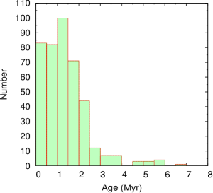
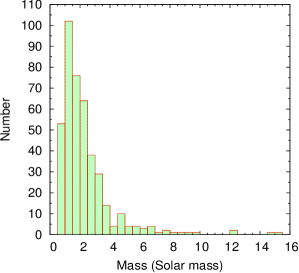
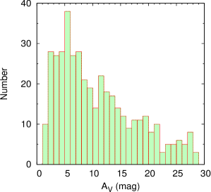
Figure 14: Histograms showing the distribution of the ages (left-hand panel), masses (center panel) and extinction values ‘$A_{V}$’ (right-hand panel) of the YSOs in the NGC 7538 region. The age, mass and $A_{V}$ are derived from the SED fitting analysis (cf. Section 3.4.1).

Finally, the X-ray luminosities ($\rm{L_{X}}$) for all 91 sources were estimated from the X-ray fluxes by using the distance of NGC 7538, i.e., 2.65 kpc. The spectral parameters of these YSOs are given in Table 7. The N_H value for these X-ray sources are in the range of $0.4-4.6\times 10^{22}~{}\rm cm^{-2}$, which corresponds to an $A_{V}$ range of 2 - 24 mag ($\rm N_{H}$ = 1.87 $\times$ 10${}^{21}A_{V}$, Bohlin et al., 1978), which is comparable to the $A_{V}$ range of the YSOs in the present study (cf. Section 4.1). Therefore, we can safely assume that these sources are the members of the NGC 7538 SFR.

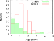
Figure 15: (Left-hand panel): Cumulative distribution of Class I (solid line) and Class II (dotted line) sources as a function of their age. (Right-hand panel): Age distribution of Class I (filled histogram) and Class II (un-filled histogram) sources.

4 Discussion

4.1 Stellar parameters and X-ray properties of the candidate YSOs

In section 3.2.1, we have determined stellar parameters of 463 YSOs using the SED fitting method. The YSOs which fall outside the distance range between 2.53 and 2.77 [i.e., $\rm(D_{s}+\sigma_{s})<(2.65-0.12)~{}kpc$ or $\rm(D_{s}-\sigma_{s})>(2.65+0.12)~{}kpc$] as well as those which have very low $A_{V}$ value [i.e., $A_{V_{s}}+\sigma_{A_{V_{s}}}<$ 2.8-0.2 mag were considered as non-members. In the above D_s and $\sigma_{s}$ are the distance and its error and 2.65 and 0.12 are the corresponding values in kpc and 2.8 and 0.2 are the foreground extinction and its error in magnitude of the NGC 7538 region (cf. Appendix A). A total of 44 sources have been found to be foreground/background populations and mistaken as associated YSOs and these are not used in further analyses. Therefore, we have selected the remaining 419 YSOs as probable members of the NGC 7538 SFR (cf. Table 6). Histograms of the age, mass and $A_{V}$ of these YSOs are shown in Fig. 14. It is found that $\sim$91% (380/419) of the sources have ages between 0.1 to 2.5 Myr. Similar results have been reported by Puga et al. (2010) and Balog et al. (2004). The masses of the YSOs are between 0.5 to 15.2 M_⊙, a majority ($\sim$86%) of them being between 0.5 to 3.5 M_⊙. These age and mass are comparable with those of TTSs. Here it is worthwhile to note that the derived masses of four YSOs are significantly higher than the cut-off limit of 8 M_⊙ for which one cannot separate observationally the luminosity due to accretion from the intrinsic luminosity of the protostar (Ward-Thompson & Whitworth, 2011). The $A_{V}$ distribution shows a long tail indicating its large spread from $A_{V}$=1 - 30 mag, which is consistent with the nebulous nature of this region. The average age, mass and extinction ($A_{V}$) for this sample of YSOs are 1.4 Myr, 2.3 M_⊙ and 11 mag, respectively.

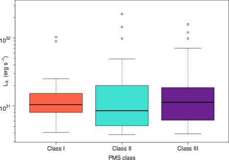
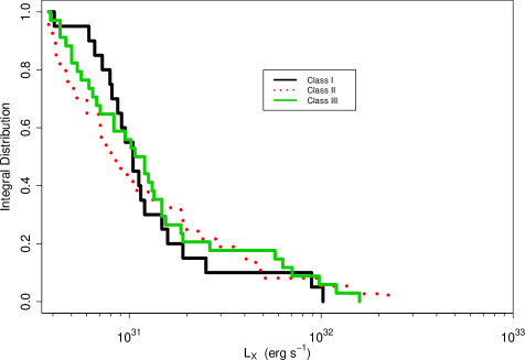
Figure 16: (Left-hand panel): Boxplots of X-ray activity of Class I, Class II and Class III objects. Data inferred from the upper and lower quartile is shown with a box and its range, denoting any points that fall outside this range as open circles. Open circles are the points outside 5 times the interquartile range above the upper quartile and below the lower quartile. (Right-hand panel): Comparison of the XLFs of Class I, Class II and Class III objects.

The evolutionary class of the selected 419 YSOs given in the Table 6 reveals that $\sim$24% (99), $\sim$62% (258) and $\sim$2% (10) sources are Class I, Class II and Class III YSOs, respectively. Remaining 52 of them could not be classified in the present study (cf. Section 3.1.2). The high percentage of Class I/II YSOs indicates the youth of this region. In Fig. 15 (left-hand panel), we have shown the cumulative distribution of Class I and Class II YSOs as a function of their ages, which manifests that Class I sources are relatively younger than Class II sources as expected. We have performed a Kolmogorov-Smirnov (KS) test for this age distribution. The test indicates that the chance of the two populations having been drawn from the same distribution is $\sim$2%. The right-hand panel of Fig. 15 plots the distribution of ages for the Class I and Class II sources. The distribution of the Class I sources shows a peak at a very young age, i.e., $\lesssim$0.5 Myr, whereas that of the Class II sources peaks at $\sim$1-1.5 Myr. Both of these figures were generated for the YSOs having masses greater than the completeness limit of this sample (i.e. $>$0.8 M_⊙) and show an age difference of $\sim$1 Myr between the Class I and Class II sources. Here it is worthwhile to take note that Evans et al. (2009) through c2d $Spitzer$ Legacy projects studied YSOs associated with five nearby molecular clouds and concluded that the life time of the Class I phase is 0.54 Myr. The peak in the histogram of Class I sources agrees well with them.

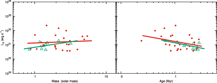
Figure 17: $L_{X}$ versus mass/age in a logarithmic scale for the identified TTSs. Red dots and green triangles represent Class II and Class III YSOs, respectively. Red and green lines are the least square fit to the data for Class II and Class III sources, respectively.

Table 8: Results of two sample tests. Columns 2, 3 and 4 represent the probability that the samples have a common parent $\rm{L_{X}}$ distribution

Test	Class I	Class II	Class I
	versus	versus	versus
	Class II	Class III	Class III
Wilcoxon Rank Sum	0.35	0.44	0.91
Peto and Peto Generalized	0.36	0.44	0.91
Wilcoxon
Kolmogorov-Smirnov	0.19	0.91	0.68
Anderson-Darling	0.16	0.44	0.43

The stellar parameters of the X-ray emitting sources identified as YSOs can be used to study the possible physical origin of the X-ray emission in PMS stars. The coronal activity which is primarily responsible for the generation of X-ray in low mass stars may be affected by the composition of X-ray emitting plasma and the disk fraction during the PMS evolution in different classes of YSOs. A number of studies have been done in various SFRs, but no firm conclusion has been drawn so far on account of contradictory results. In some cases, such as Chameleon I (Feigelson et al., 1993), $\rho$ Ophiuchus (Casanova et al., 1995), IC 348 (Preibisch & Zinnecker, 2002) and NGC 1893 (Pandey et al., 2014), no significant difference has been found in the X-ray luminosity between Class II and Class III YSOs. However, there are several examples (Stelzer & Neuhäuser, 2001a; Flaccomio et al., 2003b; Stassun et al., 2004; Preibisch et al., 2005a; Flaccomio et al., 2006; Telleschi et al., 2007b; Guarcello et al., 2012a) which show that Class II YSOs have lower X-ray luminosities than Class III YSOs.

We have derived $L_{X}$ for 91 YSOs in the NGC 7538 region (cf. Section 3.3). A comparison of the X-ray activity of the YSOs with different classes [Class I: 20, Class II: 34 and Class III: 37] are represented in Fig. 16 with boxplots and X-ray luminosity functions (XLFs) by using the Kaplan Meier estimator of integral distribution functions in the R package (ver 3.2.0). The distribution shows that the X-ray activity is nearly similar in all YSO classes with a mean value of $\rm{log(L_{X})}$ around 31.1 $\rm{erg~{}s^{-1}}$. The distribution of the Class II YSOs shows a relatively larger scatter in comparison to those of the Class I and Class III sources. To derive the statistical significance of the comparison, we performed the two sample tests for estimating the probability of having common parent distributions and the results are given in Table 8. They show that the X-ray activity in the Class I, Class II and Class III objects is not significantly different from each other. It is thought that the X-ray activity in low mass stars is associated mainly with the rotation rate and depth of the convection zone. Our results may imply that the increase of the X-ray surface activity with an increase of the rotation rate may be compensated by the decrease of the stellar surface area during the PMS evolution (Preibisch, 1997; Bhatt et al., 2013).

Out of the 91 YSOs having $L_{X}$ estimation (cf. Section 3.3), the age and mass have been estimated for 47 YSOs on the basis of SED fitting. The masses of these YSOs is $>$0.8 M_⊙. It is worthwhile to mention that the completeness limit for the X-ray emitting YSOs (64) is 0.8 M_⊙ (cf. Section 3.1.5).

To study the effect of circumstellar disks on the X-ray emission, in Fig. 17 we have tried to see if any correlation of $L_{X}$ exists with the age and mass. When concluding any results from these distributions, we have to be careful about the large errors in the estimated values of the age/mass of the TTSs.

Table 9: Coefficients of the straight lines fitted to the $L_{X}$ versus mass/age distribution of the YSOs of different classes.

Class	Mass	a	b	Age	a	b
	(M⊙)			(Myr)
II	0.9 - 5.5	$31.1\pm 0.2$	$0.2\pm 0.5$	$0.2-2.8$	$31.2\pm 0.1$	$-0.7\pm 0.4$
III	0.9 - 3.2	$30.8\pm 0.1$	$0.8\pm 0.5$	$0.7-2.8$	$31.1\pm 0.1$	$-0.8\pm 0.3$

The $L_{X}$ versus mass distribution show a large scatter but with an indication of increasing $L_{X}$ with mass for the Class III sources. The values of coefficients ‘a’ and ‘b’ of the linear regression fit log($L_{X}$) = a + b$\times$log(M_⊙) for the Class II and Class III sources are given in Table 9. The intercepts ‘a’ for the sources of different classes have comparable values to each other, indicating that the presence of circumstellar disks has practically no influence on the X-ray emission. This result is in agreement with that reported by Feigelson et al. (2002a) and Pandey et al. (2014), and is in contradiction with those by Stelzer & Neuhäuser (2001b), Preibisch et al. (2005b) and Telleschi et al. (2007a). There is an indication for a higher value of ‘b’ for Class III as compared to Class II sources. Recently, Pandey et al. (2014) have found, for their sample of Class II and Class III sources in the mass range 0.2-2.0 M_⊙ in the NGC 1893 region, the ‘b’ values to be $0.51\pm 0.20$ and $1.13\pm 0.13$, respectively, whereas the ‘a’ values to be $30.71\pm 0.07$ and $30.74\pm 0.05$, respectively. Telleschi et al. (2007a) have found a = $30.13\pm 0.09$ and $30.57\pm 0.09$ and b = $1.70\pm 0.20$ and $1.78\pm 0.17$ for Class II and Class III sources, respectively, in the Taurus molecular cloud. These slope values are higher than that obtained in the present study. One possible reason for the lower value for the NGC 7538 region may be a bias in our sample toward X-ray luminous, low mass stars. In the case of NGC 2264, the linear fit for the detected sources yields a =$30.6\pm 0.3$ and b = $0.8\pm 0.1$ (Dahm et al., 2007). However, after taking into account the X-ray non-detections, the slope is found to be steeper (b = $1.5\pm 0.1$). The mass range of YSOs used for the fitting also plays a crucial role as already demonstrated by Guarcello et al. (2012b). They have found that for Class III sources having mass $\leq$0.8 M_⊙ in NGC 6611 gave a value of slope b = $1.1\pm 0.3$, whereas the distribution of stars more massive than 0.8 M_⊙ is flatter with a slope of $0.4\pm 0.2$.

As for the $L_{X}$ versus age distribution, $L_{X}$ for both Class II and Class III sources can be seen to decrease systematically with age (in the age range of $\sim$0.4 to 2.8 Myr). The values of the coefficients ‘a’ and ‘b’ of a linear regression fit log($L_{X}$) = a + b$\times$log(age) for the sources of different classes are given in Table 9. The nearly similar values of intercept ‘a’ and slope ‘b’ for Class II and Class III indicate that circumstellar disks have practically no effect on the X-ray emission. Recently, Pandey et al. (2014) have found a = $35.06\pm 0.63$ and $35.29\pm 0.65$ and b = $-0.78\pm 0.10$ and $-0.81\pm 0.11$, respectively, for their sample of Class II and Class III sources in NGC 1893. In NGC 7538 we found that the values of ‘a’ for both Class II and Class III are much lower than those of NGC 1893, but the ‘b’ values are almost similar to theirs. These are slightly steeper in comparison to those (-0.2 to -0.5) reported by Preibisch & Feigelson (2005) and Telleschi et al. ($-0.36\pm 011$; 2007a). This difference in the slope could be more significant in the case of an unbiased sample where we expect more less luminous, low mass X-ray sources which would give a higher value for the slope. If X-ray luminosities of accreting PMS stars are systematically lower than non-accreting PMS stars (e.g., Flaccomio et al., 2003a; Preibisch et al., 2005b) and if Class II sources evolve to Class III sources, one might expect that in the case of the Class II source, $L_{X}$ should increase with age rather than decrease. However, the evolution of the Class II sources up to $\sim$2.8 Myr does not show any sign of increase in X-ray luminosity.

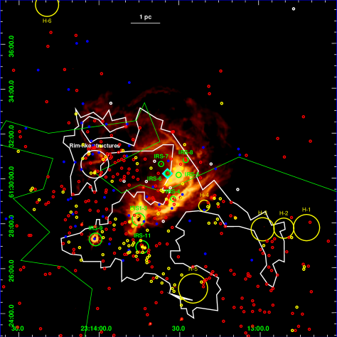
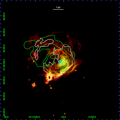
Figure 18: (Left-hand panel): Spatial distribution of the YSOs superimposed on the $15^{\prime}\times 15^{\prime}$ IRAC 8.0 $\mu$m image of the NGC 7538 region. The location of Class I (yellow circles), Class II (red dots), Class III (white dots) and unclassified (blue dots) sources are shown along with the $J=1-0$ line of ¹³CO (green contour) and 850 $\mu$m continuum emission (white contour) taken from Chavarría et al. (2014). Also shown are the positions of high-mass dense clumps (Fallscheer et al., 2013) along with the IR sources. (Right-hand panel): Distributions of the ionized gas as traced by radio (1280 MHz, green contours, Ojha et al., 2004b) and by H$\alpha$ emission (white contours) are shown overlaid on the IRAC 8.0 $\mu$m image of the same region.

.

4.2 Triggered star formation

McCaughrean et al. (1991) have suggested the presence of YSOs of various evolutionary stages in the vicinity of NGC 7538 with considerable substructures (cf. Fig. 1). Brief description of each of them is summarized as follows:

IRS 1-3: This active region has three massive IR sources, each associated with its own compact H II region (Wynn-Williams et al., 1974). IRS 1 has been identified as a high-mass ($\sim$30 M_⊙) protostar with a CO outflow, and is considered as the source injecting energy to the UC H II region NGC 7538 A (Puga et al., 2010). IRS 2, situated $\sim$10 arcsec north of IRS 1, is inferred to be an O9.5V star and possesses the most extended H II region. IRS 3 is situated about $\sim$15 arcsec west of IRS 1 (Ojha et al., 2004b) and is the least luminous of the three.

IRS 4-8: The composition of this active region is a group of young stars located at the southern rim of the optical H II region IRS 4, a bright NIR reflection nebula containing an O9V star IRS 5, and the main ionizing source IRS 6 (O3V type) of the H II region NGC 7538 (Puga et al., 2010). IRS 7 and IRS 8 have been inferred as foreground field stars (Tsujimoto et al., 2005; Puga et al., 2010).

IRS 9: This bright reflection nebula located at the south-eastern tip of NGC 7538 harbors massive protostars (Werner et al., 1979; Pestalozzi et al., 2006; Puga et al., 2010).

IRS 11: This may be a large contracting or rotating filament that is fragmenting at scales of 0.1 pc to 0.01 pc to form multiple high-mass stars ($\sim$10 M_⊙) having disks and envelopes as well as shedding outflows (Pestalozzi et al., 2006; Naranjo-Romero et al., 2012).

Rim-like structures (globules): This nebular region is seen on the north-eastern side of NGC 7538 consisting two cone-shaped rim-like structures. Both point toward IRS 6 and have faint stars on their tip.

Apart from these active regions, Fallscheer et al. (2013) have recently detected 13 more candidates for high-mass dense clump in a one square degree field of NGC 7538. The positions and sizes of some of them are shown in Fig. 1 as H1 to H6, located mainly in the south-western periphery of NGC 7538. These are potential sites of intermediate- to high-mass star formation to be identified through far infra-red (FIR) observations by $Herschel$ space based telescope.

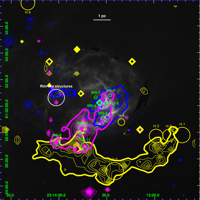
Figure 19: Distribution of younger (yellow contours), older (blue contours) and massive (purple contours) populations overlaid on the IRAC 8.0 $\mu$m image. The location of the IR sources, globules and cold clumps are also shown.

Fig. 18 (left-hand panel) shows the spatial distribution of member YSOs (419 sources, cf. Section 4.1) superimposed on the IRAC 8.0 $\mu$m image of $15\times 15$ arcmin² of the NGC 7538 region. This sample of YSOs is obtained from multiwavelength data taken from various surveys having different completeness limits. In section 3.1.5, we have discussed the completeness of these surveys and found that approximately they can be assumed complete for mass $\geq$0.8 M_⊙. A majority (94%) of the YSOs selected here have masses $\geq$0.8 M_⊙, therefore, incompleteness in this sample will have minimal effect on the over-all spatial distribution of the YSOs.

The ¹³CO $J=1-0$ line (green contour) and 850 $\mu$m continuum (white contour) emission maps taken from Chavarría et al. (2014) are shown in Fig. 18 (left-hand panel). For simplicity we have shown only the outer most contours, representing the extent of gas and dust in this region. The resolution of the ¹³CO and 850 $\mu$m observations are 46 arcsec and 14 arcsec, respectively. Chavarría et al. (2014) have studied the groupings of YSOs in this region and found several of them. They estimated physical parameters of these groups and found that younger sources are located in regions having higher YSOs surface density and are correlated with densest molecular clouds. Since they have not discussed the effect of high mass stars on the recent star formation through the distribution of YSOs, gas and dust, we further used these distributions to trace star formation activities in this region. The positions of the high-mass dense clumps (Fallscheer et al., 2013) along with the IR sources are also shown in the figure. In the right-hand panel of Fig. 18, the distributions of ionized gas as seen in the 1280 MHz radio continuum emission (green contours, Ojha et al., 2004b) and in H$\alpha$ emission (white contours) are shown superposed on the IRAC 8.0 $\mu$m image of the same region. The YSOs are distributed either on the nebulosity or towards the southern regions. The distribution of the ¹³CO, 850 $\mu$m and H$\alpha$ emission indicates a bubble-like feature around the ionizing source IRS 6, likely created due to the expansion of the H II region. The correlation of the PAH emission as seen in IRAC 8.0 $\mu$m image (Pomarès et al., 2009) with the ¹³CO emission indicates that the ionized gas is confined inside the molecular cloud. The lack of diffuse emission at 8.0 $\mu$m can be noticed towards the south-east of IRS 6. However, as can be seen from the radio continuum contours in Fig. 18 (right-hand panel), the ionized gas is bounded more sharply to the south-western region. The distribution of Class I YSOs shows a nice correlation with that of molecular gas and the PAH emission/H II region boundaries. Very few Class I sources are located towards the central region near IRS 6 as compared to the outer, southern regions. The strong positional coincidence between the YSOs and the molecular cloud suggests an enhanced star formation activity towards this region, as often observed in other SFRs (e.g. Evans et al., 2009; Fang et al., 2009). There is a concentration of very young YSOs (mainly Class I) towards the southern region outside of the dust rim (IRS 11). Five high-mass dense clump candidates (Fallscheer et al., 2013) are located just outside the NGC 7538 H II region towards southwest. There are many separate groups of younger YSOs located near these cold molecular clumps. In summary, there are two main concentrations of YSOs, one in the H II region and the other in the southern region.

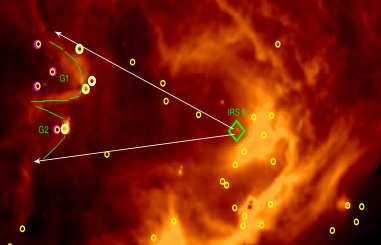
Figure 20: Location of the two globules along with the distribution of Class I YSOs (circles) and ‘IRS 6’, the ionizing source of NGC 7538.

By analyzing the distribution of YSOs of various ages and masses in relation to the molecular cloud structure, we can study the mode of star formation in this region. For this, we have generated contour maps of the age/mass of YSOs smoothened to the resolution of 9 arcsec grid size. In Fig. 19, we have over-plotted the age contours on the IRAC 8.0 $\mu$m image representing younger (yellow contours) and comparatively older (blue contours) YSOs. The outermost age contours for them correspond to 0.7 Myr and 1.8 Myr, respectively. In the same figure, we have also plotted the mass contours (purple contours) of the YSOs representing the massive ones. The outer-most contour for it corresponds to 4.2 M_⊙. The step size are 0.2 Myr and 0.2 M_⊙ for the age and mass contours, respectively. The older population is mainly associated with the H II region enclosed by thick blue contours, whereas the younger one is located outside the H II region mainly in the south-western part enclosed in a thick yellow contour. The mass distribution shows that the massive population, enclosed in the thick purple contours, is sandwiched between these two populations and is associated mainly with IRS 1-3, IRS 9 and IRS 11. The mean values of ages and masses of the YSOs associated with these subregions are given in Table 10.

Table 10: Mean values of ages and masses of YSOs in different regions.

Region	N	Mean mass	Mean age
		(M⊙)	(Myr)
Whole	419	$2.3\pm 0.1$	$1.4\pm 0.1$
South-west (young)	91	$1.8\pm 0.1$	$1.0\pm 0.1$
Central (old)	73	$2.7\pm 0.2$	$2.0\pm 0.2$
"      (old-globules)	32	$2.5\pm 0.2$	$1.9\pm 0.2$
"      (old-IRS 6)	41	$2.9\pm 0.2$	$2.2\pm 0.2$
South-central (massive)	35	$4.7\pm 0.6$	$1.2\pm 0.2$

The location of the IR sources, rim-like structures and the cold clumps are also shown in Fig. 19. The oldest region (thick blue contours) is made up of two separate groups, i.e., one around IRS 6 and the other near the rim-like structures (globules). The masses and ages of the YSOs near the rim-like structures are lower as compared to those in the central region near IRS 6. The two rim-like structures with sharp edges (maybe due to the PAH emission) pointing towards the central star IRS 6 indicate that the ionization front (IF) interacts with the molecular ridge as seen in the ¹³CO emission. They morphologically resemble bright-rimmed clouds that result from the pre-existing dense molecular clouds impacted by the ultra-violet photons from nearby OB stars (Lefloch & Lazareff, 1994). The low mass YSOs on their tips are generally believed to be formed as a result of triggering effect of the expanding H II region (Deharveng et al., 2005; Zavagno et al., 2006; Koenig et al., 2008; Deharveng et al., 2009). Their elongated distribution and age difference with respect to the location of the ionization source can be used to check whether the RDI (Lefloch & Lazareff, 1994; Miao et al., 2006) mode of triggered star formation was effective in the region.

For this purpose, we have compared the time elapsed during the formation of the Class I YSOs in the globule regions with the age/lifetime of the O3 ionization source. In Fig. 20, we show the location of the two globules, the ionizing source IRS 6 and the Class I sources. The presence of extremely young Class I sources presumably represents the very recent star formation event in the region, thus can be taken as a proxy to trace the triggered star formation. The position of the tips of the globules is situated at a projected distance of $\sim$2.4 pc from IRS 6. We estimated the time needed for the IF to travel there as $\sim 0.26$ Myr, assuming that it expanded at the speed of $\sim$9 km s^-1 (see, e.g., Pismis & Moreno, 1976). The age of the Class I sources (white circles in Fig. 20) on this rim is $1.9\pm 0.6$ Myr, which is $\sim$0.3 Myr younger than the estimated age of the O3V star ($\sim$2.2 Myr, cf. Puga et al., 2010). The mean age of the Class I sources inside the rim (magenta circles in Fig. 20) is $1.5\pm 0.6$ Myr. We have evaluated the shock crossing time in the globules to see whether the star formation there initiated by the propagation of the shock or whether it had already taken place prior to the arrival of the shock. Assuming a typical shock propagation velocity of 1-2 km s^-1, as found in the case of bright-rimmed clouds (see, e.g., White et al., 1999; Thompson et al., 2004), the shock travel time to the YSOs, which are projected at distances $\sim$0.6 pc from the head, is $\sim 0.4$ Myr. This time-scale is comparable to the difference in the ages of the YSOs on the rims and inside them. Although the sample is small and the errors are large, these results seems to support the notion that the formation of the YSOs in the globules could be due to the RDI mechanism. The above analysis is not statistically significant to conclude the triggered star formation, but Dale et al. (2015) have stated that the system where many indicators can be satisfied simultaneously can be a genuine site of triggering.

Therefore, to investigate further, we have calculated the dynamical age of the NGC 7538 H II region from its radius using the equation given by Spitzer (1978):

Figure 21: Plots showing the variation of the Strömgren radius and dynamical age with the ambient density.

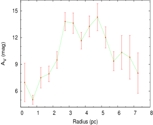
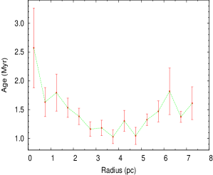
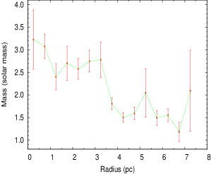
Figure 22: Distribution of $A_{V}$, age and mass of the YSOs as a function of radial distance from the ionizing source IRS 6.

$R(t)=R_{S}(1+{{7ct}\over{4R_{s}}})^{4/7}$,

where $R(t)$ denotes the radius of the H II region at time $t$, and $c$ is the sound speed. The latter was assumed as $\sim$9 km s^-1 (Pismis & Moreno, 1976; Stahler & Palla, 2005), and the former was taken to be 3 pc as is derived from the radio and H$\alpha$ maps (cf. Fig. 18). Then the dynamical age $(t)$ can be calculated if we know Strömgren radius $R_{S}$, which is estimated by using the relation given in Ward-Thompson & Whitworth (2011) and Stahler & Palla (2005) and by assuming an O3V star as the ionizing source emitting 7.4 $\times 10^{49}$ UV photons per second (Vacca et al., 1996). However, the information on the initial ambient density is needed, which we don’t know. So we have left it as a free parameter and calculated the Strömgren radius ($R_{S}$) and the corresponding dynamical age $(t)$ of the H II region for a range of ambient density from $10^{3}$ to $10^{4}$ cm^-3. Fig. 21 shows the results, where $R_{S}$ and $t$ are plotted as a function of the initial ambient density. The former varies from $\sim$ 1.3 to 0.25 pc, while the latter varies from $\sim$ 0.7 to 2.6 Myr. This upper limit of the dynamical age is comparable to the age of the central O3 star and corresponds to a higher ambient density for this region. The mean age of the YSOs in this region is 1.4 Myr, which is less than the dynamical age of the region and, as such, their formation could have been influenced by the expanding H II region.

We have also looked for the radial distance dependence of $A_{V}$/age/mass of YSOs with respect to the ionizing source IRS 6 as shown in Fig. 22. As expected, the $A_{V}$ distribution reveals less extinction near IRS 6 as compared to the outer region. There is a broad peak starting at the projected distance of $\sim$3 pc and we see a decreasing trend after 5 pc. This seems to indicate the presence of a shell-like layer of collected medium just outside the H II region. It is very interesting to note that the age distribution shows a clear decrease from the center to a distance of 3 pc. Also the masses of the YSOs within 3 pc is higher as compared to those outside indicating a difference in the physical properties of the YSOs within 3 pc. These trends are indicative of triggered star formation in the inner region (within 3 pc), where the O3 star played an active role. From 3 pc out, we see a completely different distribution with a large number of young and low mass YSOs (cf. Table 10) located in the southwest region of NGC 7538 (cf. Fig. 19, thick yellow contour). It seems that the YSOs in this group might have formed spontaneously in the absence of any triggering mechanism due to the O3 star. The distribution of the cold clumps also suggests that spontaneous low-mass star formation is under way there. However, disentangling triggered star formation from spontaneous star formation accurately requires precise determination of the proper motions and ages of individual sources (Dale et al., 2015).

4.3 Mass function

The distribution of stellar masses that form in one star-formation event in a given volume of space is called IMF. Together with star formation rate, it is one of the important issues of star-formation studies. Since, environment effects due to the presence of high mass stars may be more revealing at the low-mass end of the present day MF, we will try to study it in the NGC 7538 SFR.

The MF is often expressed by a power law, $N(\log m)\propto m^{\Gamma}$ and the slope of the MF is given as:

$$\Gamma=d\log N(\log m)/d\log m$$

where $N(\log m)$ is the number of stars per unit logarithmic mass interval. The first empirical determination of MF was by Salpeter (1955), which gave $\Gamma=-1.35$ for the field stars in the Galaxy in the mass range $0.4\leq$ m/M${}_{\odot}\leq 10$. However, subsequent works (eg. Miller & Scalo, 1979; Scalo, 1986; Rana, 1991; Kroupa, 2002) suggest that the MF in the Galaxy often deviates from the pure power law. It has been shown (see e.g. Scalo, 1986, 1998; Kroupa, 2002; Chabrier, 2003; Corbelli et al., 2005) that, for masses above $\sim$1 M_⊙, the MF can generally be approximated by a declining power law with a slope similar to that found by Salpeter (1955). However, it is now clear that this power law does not extend to masses below $\sim$1 M_⊙. The distribution becomes flatter below 1 M_⊙ and turns down at the lowest stellar masses. Kroupa (2002) divided the MF slopes for four different mass intervals. It was also often claimed that some (very) massive SFRs have truncated MFs, i.e., contain much smaller numbers of low-mass stars than expected from the field MF. However, most of the recent and sensitive studies of massive SFRs (see, e.g. Liu et al., 2009; Espinoza et al., 2009) found large numbers of low-mass stars in agreement with the expectation from the “normal" field star MF. Preibisch et al. (2011) confirmed these results for the Carina Nebula and supported the assumption of a universal IMF (at least in our Galaxy). In consequence, this result also supports the notion that OB associations and massive star clusters are the dominant supply sources for the Galactic field star population, as already suggested by Miller & Scalo (1978).

Figure 23: $V/(V-I_{c})$ CMD for (a) stars in the NGC 7538 region and (b) stars in the reference region. (c) is a statistically cleaned CMD.

As discussed earlier the sample of YSOs used is compiled from various surveys having different completeness limits. So we have tried to use only our deep and homogeneous optical data to generate the MF of the NGC 7538 region (cf. Sharma et al., 2007; Pandey et al., 2008; Chauhan et al., 2011; Pandey et al., 2013; Jose et al., 2013). For this, we have utilized the optical $V$ versus $(V-I_{c})$ CMD of all the sources in the NGC 7538 FOV and that of the nearby field region of equal area and decontaminated the former sources from foreground/background stars using a statistical subtraction method. In Fig. 23, we have shown the $V/(V-I_{c})$ CMDs for the stars lying within the NGC 7538 FOV (left panel) and for those in the reference field region (middle panel). To statistically subtract the latter from the former, the both CMDs were divided into grids of $\Delta V=1$ mag by $\Delta(V-I_{c})=0.4$ mag. The number of stars in each grid of the both CMDs were then counted and the probable number of cluster members in each grid were estimated from the difference. The estimated numbers of contaminating field stars (the numbers in the bin - the probable numbers of cluster members) were removed from the cluster CMD one by one that is the nearest to the randomly selected star in the CMD of the reference region of that bin. The both CMDs were also corrected for the incompleteness of the data. The photometric data may be incomplete due to various reasons, e.g., nebulosity, crowding of the stars, detection limit etc. In particular it is very important to know the completeness limits in terms of mass. The $IRAF$ routine $ADDSTAR$ of $DAOPHOTII$ was used to determine the completeness factor (CF) (for detail, see Sharma et al., 2008). Briefly, in this method artificial stars of known magnitudes and positions are randomly added in the original frames and then these artificially generated frames are re-reduced by the same procedure as used in the original reduction. The ratio of the number of stars recovered to those added in each magnitude gives the CF as a function of magnitude. To determine the completeness of the $V$ versus $(V-I_{c})$ CMD, we followed the procedure given by Sagar & Richtler (1991) by adding artificial stars to both $V$ and $I$ images in such a way that they have similar geometrical locations but differ in $I$ brightness according to the mean $(V-I_{c})$ colours of the MS stars. Since the mean $(V-I_{c})$ colour of the MS stars is $\sim$2 mag in the NGC 7538 region (cf. Fig. 23), the $I$ band magnitude is offset-ed to the $V$ band magnitude by adding a correction of $\sim$2 mag in Fig. 24 showing the CF as a function of magnitudes. As expected the CF decreases with fainter magnitudes. Our photometry is more than 90% complete up to V$\simeq$21.5 mag, which corresponds to the detection limit of a 0.8 M_⊙ (cf. Fig. 25) PMS star of $\simeq$1.8 Myr age embedded in the nebulosity of $A_{V}\simeq$3.0 mag (i.e., the average values for the optically detected YSOs, cf. Table 6).

In Fig. 25, we have plotted the statistically cleaned $V/(V-I_{c})$ CMD for the NGC 7538 region showing the presence of PMS stars in the region. We have also plotted the ZAMS by Siess et al. (2000) and the PMS isochrones by Siess et al. (2000). The evolutionary tracks by Siess et al. (2000) for various masses have also been plotted. The dashed horizontal line represents the completeness limit of the data at $(V-I_{c})$ = 2 mag after taking into account the average extinction of the YSOs corrected for the distance.

The masses of individual stars were then estimated by the same technique mentioned in Section 3.2.2, and the corresponding MF has been plotted in Fig. 26 (upper panel). For this, we have used only those sources which have ages equivalent to the average age of the optically identified YSOs combined with error (i.e., $\leq$3.5 Myr, cf. Table 6). There is a change of slope from the high mass to low mass end with a turn-of at around 1.5 M_⊙, as has often been noticed in other regions (Sharma et al., 2007; Pandey et al., 2008; Jose et al., 2008). The slope of the MF $\Gamma$ for this sample in the mass range $\sim 1.5<$M/M${}_{\odot}<6$ comes out to be $-1.76\pm 0.24$, which is steeper than the value -1.35 given by Salpeter (1955). We have optical photometry of only two IR sources associated with the NGC 7538 region, i.e., IRS 5 (O9, 20 M_⊙) and IRS 6 (O3, 60 M_⊙) as others could not be resolved or are foreground sources. For the generation of the MF, we have not used these two stars as they will introduce large gaps between the points in the MF distribution and corresponding errors will be quite large. Also, a lower mass range is required to compare this MF distribution to that of YSOs.

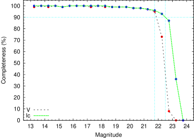
Figure 24: Completeness levels for $V$ and $I_{c}$ (off-setted by 2 mag) bands as a function of magnitude derived from the artificial star experiments (ADDSTAR, see Section 4.3).

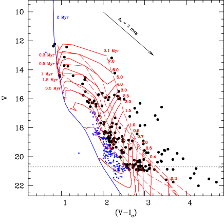
Figure 25: Statistically cleaned $V/(V-I_{c})$ CMD for stars lying in the NGC 7538 region. Filled circles (Ages $\leq$ 3.5 Myr) are used to estimate the MF of the region. The isochrone of 2 Myr by Marigo et al. (2008) and the PMS isochrones of 0.1,0.3,0.5,1,1.8,3.5 Myr along with the evolutionary tracks for different masses by Siess et al. (2000) are also shown. All the curves are corrected for the distance of 2.65 kpc and the foreground extinction $A_{V}$= 2.1 mag. The dashed horizontal line represents the completeness limit of the data after taking into account the average extinction of the YSOs.

Figure 26: A plot of the MF for the statistically cleaned CMD (top panel) and the identified YSOs (bottom panel) in the NGC 7538 region. Log $\phi$ represents log($N$/dlog $m$). The error bars represent $\pm\sqrt{N}$ errors. The solid line shows a least squares fit to the MF distribution (Black dots). Open squares are the data points falling below the completeness limit of 0.8 M_⊙. Open circles are the data points near turn-off point in the MF distribution and are not used in the fitting.

Since the detection limit for the optical sample is upto $A_{V}\simeq$7.7 mag (cf. Appendix A), the optical sample will represent YSOs which are on the surface or partially embedded in the nebulosity of the NGC 7538 SFR. We need NIR/MIR data to cover the deeply embedded YSOs. In Section 3.2.1, with the help of the SED fitting, we have estimated the age and mass of 419 YSOs by using mostly NIR/MIR data. Therefore, we have used this sample to trace further deep in the NGC 7538 region. The completeness limit for this sample, where the data of individual YSOs are taken from various surveys, is discussed in section 3.1.5 and found to be 0.8 M_⊙. The masses of the YSOs in this sample were used to generate the MF and is shown in the lower-panel of Fig. 26 (see also, Kumar et al., 2014; Yadav et al., 2016). We have not used here the four high mass YSOs (cf. Section 4.1). The slope of the MF $\Gamma$ down to a similar mass limit (i.e. 1.5 M_⊙) for this sample of YSOs comes out to be $-1.56\pm 0.27$, which is similar within the error with that derived by using optical CMD. From this, we can infer that the optical and SED fitting samples represent the same population of YSOs.

5 Conclusion

Although the NGC 7538 region has already been studied extensively in IR and radio wavelengths, it is rather neglected in the optical and X-ray. To the best of our knowledge, the present study is the first detailed multiwavelength study (including the optical) of this region. We have added some more YSOs based on their H$\alpha$ or X-ray emission, thus complemented the previous IR excess based catalog of the YSOs in the region. We have checked the association of these YSOs with NGC 7538 and derived their individual physical parameters based on the SED fitting. The spatial distribution of these YSOs along with those of the MIR and radio emission have been used to constrain the star-formation history in the region. The XLF and MF for the YSOs in this region have also been derived. The main results of this study can be summarized as follows:

• Analysis of the $Chandra$ X-ray data in a $\approx 17\times 17$ arcmin² field of the NGC 7538 region reveals 190 X-ray emitting sources.

• On the basis of H$\alpha$ grism spectroscopy, H$\alpha$ (photometry) and X-ray emission, we have identified 6, 15 and 64 YSOs, respectively, in the region. We have compiled a catalog of 943 YSOs by combining those detected in the present study with those previously cataloged. 53 YSOs are new additions from this study. This new catalog is complete down to 0.8 M_⊙.

• We have derived the age/mass of 463 YSOs based on the SED fitting analysis. 419 of them are confirmed to belong to the NGC 7538 SFR and $\sim$91% (380/419) of them have ages between 0.1 to 2.5 Myr. A majority ($\sim$86%) of the 419 YSOs have masses between 0.5 to 3.5 M_⊙ as derived by SED fitting analysis. These ages and masses are comparable with those of TTSs. The $A_{V}$ value for these YSOs shows a spread from 1 to 30 mag. The average age, mass and extinction ($A_{V}$) for this sample of YSOs are 1.4 Myr, 2.3 M_⊙ and 11 mag, respectively.

• Of the above 419 YSOs, around 24% (99), 62% (258) and 2% (10) are found to be Class I, Class II and Class III sources, respectively. The high percentage ($\sim$85%) of Class I and Class II YSOs indicates the youth of this region. A KS test for the age distribution of the Class I and Class II sources suggests that it is different. The ages of Class I sources are $\lesssim$0.5 Myr, whereas the Class II sources have ages $\sim$1-1.5 Myr mostly, indicating an age difference of $\sim$1 Myr between them.

• The mean value of $\rm{log(L_{X})}$ of identified YSOs in the region is found to be around 31.1 $\rm{erg~{}s^{-1}}$. It is found that the X-ray activity of the Class I, Class II and Class III sources is not significantly different from each other. The $L_{X}$ seems to increase with the mass of the Class III sources, whereas it decreases with the age of the Class II and Class III sources. However, we find no statistically significant difference in the slopes and intercepts for the $L_{X}$ versus age distribution for the Class II and Class III sources, which indicates that the presence of circumstellar disks has practically no influence on the X-ray emission. This suggests that the increase of the X-ray surface activity with the increase of the rotation rate may be compensated by the decrease of the stellar surface area during the PMS evolution.

• The spatial distribution of the YSOs along with those of MIR/radio/CO emission has been used to understand the star formation process in the region. The YSOs in the inner region (within 3 pc from IRS 6, containing the bright H II region) may have been formed by a triggering mechanism caused by the central high mass star IRS 6.

• The MF changes its slopes from high mass to low mass sides with a turn-off at around 1.5 M_⊙. The slope of the MF $\Gamma$ in the mass range $1.5<$M/M${}_{\odot}<6$ comes out to be $-1.76\pm 0.24$, which is steeper than the Salpeter (1955) value -1.35.

Appendix A Distance and reddening of NGC 7538

NGC 7538 is located in the second quadrant of the Galaxy in the Perseus arm. Its distance estimates in literature ranges from 2.2 kpc (Moreno & Chavarria-K., 1986) to 2.8 kpc (Crampton et al., 1978). The accuracy of these photometrically determined distances are typically 10%-20%. Puga et al. (2010) reported a spectro-photometric distance of 2.7 $\pm$ 0.5 kpc to this region. Moscadelli et al. (2009), using the trigonometric parallaxes of methanol masers which are usually associated with high-mass SFRs, derived a most accurate distance of this region as 2.65${}^{+0.12}_{-0.11}$. Therefore, we have adopted 2.65 kpc as the distance for NGC 7538 in our analyses.

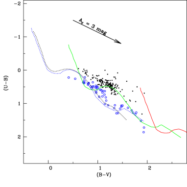
Figure 27: $(U-B)/(B-V)$ TCD for the sources in the NGC 7538 region. The dotted blue curve represents the intrinsic ZAMS for $Z=0.02$ by Schmidt-Kaler (1982) along with the selected foreground stars (blue open circles). 1 Myr isochrone (equivalent to ZAMS) from Marigo et al. (2008) is also shown as black dotted curve. The continuous curves represent the Schmidt-Kaler (1982) ZAMS shifted along the reddening vector (see text for details) by $E(B-V)_{min}$ = 0.75 mag (green curve) and $E(B-V)_{max}$ = 2.2 mag (red curve) for references to the stars embedded in the nebulosity of NGC 7538 (black dots).

A $(U-B)/(B-V)$ TCD has been used to estimate the amount of reddening towards the NGC 7538 region. In Fig. 27 we show the TCD with the intrinsic zero-age-main-sequence (ZAMS, blue dotted curve) taken from Schmidt-Kaler (1982) along with the identified stars (black dots). For comparison, we have also overplotted in Fig. 27, the 1 Myr isochrone (equivalent to ZAMS) from Marigo et al. (2008) which agrees well with that of Schmidt-Kaler (1982). The distribution of the stars shows a large spread along the reddening line, indicating heavy differential reddening in this region. It reveals two different populations, one (blue open circles) distributing along the ZAMS and another (black dots) showing a large spread in their reddening value. The former having negligible reddening must be the foreground population and the latter could be member stars. The both populations are selected visually on the basis of their locations with respect to the ZAMS (for detail cf., Golay, 1974; Phelps & Janes, 1994). If we look at the MIR image of the NGC 7538 region (Fig. 1), we see several dust lanes along with enhancements of nebular emission at many places; the both are likely responsible for the large spread of reddening in the latter population.

The ZAMS from Schmidt-Kaler (1982) is shifted along the reddening vector with a slope of $E(U-B)/E(B-V)$ = $0.72\times 0.91$ (corresponding to $R_{V}$ = 2.82) to match the distribution of the stars showing the minimum reddening among the member population (green curve); this gives $E(B-V)_{min}$ =0.75 and A${}_{V}\simeq$ 0.75$\times$2.82 = 2.1 mag. The others may be embedded in the nebulosity of the H II. The ZAMS is further shifted along the reddening vector with a slope of $E(U-B)/E(B-V)$ = $0.72\times 1.24$ (corresponding to $R_{V}$ = 3.85) to match the distribution of these embedded stars showing the maximum reddening value, $E(B-V)_{max}$=2.2 mag (red curve, A${}_{V}\simeq$ (0.75$\times$2.82 + 1.45$\times$3.85) = 7.7 mag). The approximate error in the reddening measurement ‘$E(B-V)$’ is 0.2 mag, as has been determined by the procedure outlined in Phelps & Janes (1994).

Appendix B Reddening Law

We have used the technique as described by Pandey et al. (2003) to study the nature of the diffuse interstellar medium (ISM) associated with the NGC 7538 region. This can be represented by the ratio of total-to-selective extinction $R_{V}$ = $A_{V}$/$E(B-V)$. The normal reddening law for the solar neighborhood gives the value $R_{V}$ = 3.1$\pm$ 0.2 (Whittet, 2003; Guetter & Vrba, 1989; Lim et al., 2011), but in the case of several SFRs, it is found to be anomalously high (see e.g., Pandey et al., 2000; Pandey et al., 2008; Hur et al., 2012; Pandey et al., 2013; Kumar et al., 2014).

The TCDs of the form of $(V-\lambda)$ versus $(B-V)$, where $\lambda$ indicates one of the wavelengths of the broad-band filters ($R,I,J,H,K,L$), provide an effective method for separating the influence of the normal extinction produced by the general ISM from that of the abnormal extinction arising within regions having a peculiar distribution of dust sizes (cf. Chini et al., 1990; Pandey et al., 2000). We have selected all the stars having optical and NIR detections and plotted their $(V-\lambda)$ versus $(B-V)$ TCDs in Fig. 28. It reveals two distributions having different slopes. Presumably, blue and black dots are the foreground population and the stars associated with NGC 7538, respectively, selected on the basis of their reddening values (cf. Appendix A). Since YSOs (open circles) show excess IR emission, their position can deviate from those of the MS stars in the above TCDs, therefore they have not been used in the calculation of the reddening law. The slopes of the least square fit to the distribution of the MS member stars (black dots) in the $(V-I_{c}),(V-J),(V-H)$ and $(V-K)$ versus $(B-V)$ TCDs are found to be $1.44\pm 0.04,2.47\pm 0.07,2.95\pm 0.07$ and $3.03\pm 0.06$, respectively, which are higher than those found for the general ISM (1.10, 1.96, 2.42 and 2.60; cf., Pandey et al., 2003). On the other hand, the field population (blue dots) gives lower values for them (i.e., $1.12\pm 0.04,1.75\pm 0.08,2.26\pm 0.07$ and $2.36\pm 0.06$).

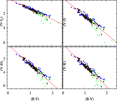
Figure 28: $(V-I_{c}),(V-J),(V-H),(V-K)$ versus $(B-V)$ TCDs for the stars associated with the NGC 7538 region (black dots) and for the foreground populations (blue dots) (cf. Appendix A). Open green circles are identified YSOs (cf. Section 3.1.4) and are not used in the analysis. Straight lines show the least-square fit to the stars in the NGC 7538 region.

The slopes for the MS stars associated with the NGC 7538 region estimated as above yield a higher value for $R_{V}$ ($\sim 3.85\pm 0.15$) (for a description on reddening law estimation, see Pandey et al., 2003), indicating larger grain sizes of the material in this region as compared to the general ISM. In many SFRs, $R_{V}$s tend to deviate from the normal value, preferably towards the higher ones, for example: $R_{V}$ = 3.7 (Kumar et al., 2014, the Carina region), $R_{V}$= 3.3 (Pandey et al., 2013, NGC 1931), $R_{V}$ = 3.5 (Sharma et al., 2012, NGC 281) and $R_{V}$ = 3.7 (Pandey et al., 2008, Be 59). Within dense dark clouds, the accretion of ice mantles on grains and the coagulation due to grain collision can change the size distribution leading to higher $R_{V}$ values (Cardelli et al., 1989). The value of $R_{V}$ for the foreground population (blue dots in Fig. 28) towards the direction of NGC 7538 comes out to be $\sim 2.82\pm 0.10$, indicating a slightly smaller grain size in the foreground medium of NGC 7538 as compared to the general ISM. It is interesting to point out that Eswaraiah et al. (2012) have reported the mean value of $R_{V}$ as $2.79\pm 0.18$ for the general ISM towards the Be 59 SFR ($l=118.22^{\circ}$, $b=5.00^{\circ}$), which is in a similar direction to NGC 7538, on the basis of polarimetric observations.

References

- Balog et al. (2004) Balog Z., Kenyon S. J., Lada E. A., Barsony M., Vinkó J., Gáspaŕ A., 2004, AJ, 128, 2942
- Balucinska-Church & McCammon (1992) Balucinska-Church M., McCammon D., 1992, ApJ, 400, 699
- Bertoldi (1989) Bertoldi F., 1989, ApJ, 346, 735
- Bessell & Brett (1988) Bessell M. S., Brett J. M., 1988, PASP, 100, 1134
- Bhatt et al. (2013) Bhatt H., Pandey J. C., Singh K. P., Sagar R., Kumar B., 2013, Journal of Astrophysics and Astronomy, 34, 393
- Bica et al. (2003) Bica E., Dutra C. M., Barbuy B., 2003, A&A, 397, 177
- Bohlin et al. (1978) Bohlin R. C., Savage B. D., Drake J. F., 1978, ApJ, 224, 132
- Briceño et al. (2007) Briceño C., Preibisch T., Sherry W. H., Mamajek E. A., Mathieu R. D., Walter F. M., Zinnecker H., 2007, Protostars and Planets V, pp 345–360
- Broos et al. (2010) Broos P. S., Townsley L. K., Feigelson E. D., Getman K. V., Bauer F. E., Garmire G. P., 2010, The Astrophysical Journal, 714, 1582
- Caramazza et al. (2012) Caramazza M., et al., 2012, A&A, 539, A74
- Cardelli et al. (1989) Cardelli J. A., Clayton G. C., Mathis J. S., 1989, ApJ, 345, 245
- Carpenter et al. (1993) Carpenter J. M., Snell R. L., Schloerb F. P., Skrutskie M. F., 1993, ApJ, 407, 657
- Casanova et al. (1995) Casanova S., Montmerle T., Feigelson E. D., Andre P., 1995, ApJ, 439, 752
- Chabrier (2003) Chabrier G., 2003, PASP, 115, 763
- Chauhan et al. (2009) Chauhan N., Pandey A. K., Ogura K., Ojha D. K., Bhatt B. C., Ghosh S. K., Rawat P. S., 2009, MNRAS, 396, 964
- Chauhan et al. (2011) Chauhan N., Pandey A. K., Ogura K., Jose J., Ojha D. K., Samal M. R., Mito H., 2011, MNRAS, 415, 1202
- Chavarría et al. (2014) Chavarría L., Allen L., Brunt C., Hora J. L., Muench A., Fazio G., 2014, MNRAS, 439, 3719
- Chini et al. (1990) Chini R., Kruegel E., Kreysa E., 1990, A&A, 227, L5
- Cohen et al. (1981) Cohen J. G., Persson S. E., Elias J. H., Frogel J. A., 1981, ApJ, 249, 481
- Corbelli et al. (2005) Corbelli E., Palla F., Zinnecker H., eds, 2005, The Initial Mass Function 50 years later Astrophysics and Space Science Library Vol. 327
- Crampton et al. (1978) Crampton D., Georgelin Y. M., Georgelin Y. P., 1978, A&A, 66, 1
- Currie et al. (2009) Currie T., Evans N. R., Spitzbart B. D., Irwin J., Wolk S. J., Hernandez J., Kenyon S. J., Pasachoff J. M., 2009, AJ, 137, 3210
- Cutri et al. (2003) Cutri R. M., et al., 2003, VizieR Online Data Catalog, 2246, 0
- Dahm et al. (2007) Dahm S. E., Simon T., Proszkow E. M., Patten B. M., 2007, AJ, 134, 999
- Dale et al. (2015) Dale J. E., Haworth T. J., Bressert E., 2015, MNRAS, 450, 1199
- Damiani et al. (1997) Damiani F., Maggio A., Micela G., Sciortino S., 1997, ApJ, 483, 350
- Deharveng et al. (2005) Deharveng L., Zavagno A., Caplan J., 2005, A&A, 433, 565
- Deharveng et al. (2009) Deharveng L., Zavagno A., Schuller F., Caplan J., Pomarès M., De Breuck C., 2009, A&A, 496, 177
- Deharveng et al. (2010) Deharveng L., et al., 2010, A&A, 523, A6
- Dutta et al. (2015) Dutta S., Mondal S., Jose J., Das R. K., Samal M. R., Ghosh S., 2015, MNRAS, 454, 3597
- Elmegreen (1998) Elmegreen B. G., 1998, in Woodward C. E., Shull J. M., Thronson Jr. H. A., eds, Astronomical Society of the Pacific Conference Series Vol. 148, Origins. p. 150 (arXiv:astro-ph/9712352)
- Elmegreen & Lada (1977) Elmegreen B. G., Lada C. J., 1977, ApJ, 214, 725
- Espinoza et al. (2009) Espinoza P., Selman F. J., Melnick J., 2009, A&A, 501, 563
- Eswaraiah et al. (2012) Eswaraiah C., Pandey A. K., Maheswar G., Chen W. P., Ojha D. K., Chandola H. C., 2012, MNRAS, 419, 2587
- Evans et al. (2009) Evans II N. J., et al., 2009, ApJS, 181, 321
- Fallscheer et al. (2013) Fallscheer C., et al., 2013, ApJ, 773, 102
- Fang et al. (2009) Fang M., van Boekel R., Wang W., Carmona A., Sicilia-Aguilar A., Henning T., 2009, A&A, 504, 461
- Favata & Micela (2003) Favata F., Micela G., 2003, Space Sci. Rev., 108, 577
- Feigelson & Montmerle (1999a) Feigelson E. D., Montmerle T., 1999a, ARA&A, 37, 363
- Feigelson & Montmerle (1999b) Feigelson E. D., Montmerle T., 1999b, ARA&A, 37, 363
- Feigelson et al. (1993) Feigelson E. D., Casanova S., Montmerle T., Guibert J., 1993, ApJ, 416, 623
- Feigelson et al. (2002a) Feigelson E. D., Broos P., Gaffney III J. A., Garmire G., Hillenbrand L. A., Pravdo S. H., Townsley L., Tsuboi Y., 2002a, ApJ, 574, 258
- Feigelson et al. (2002b) Feigelson E. D., Broos P., Gaffney III J. A., Garmire G., Hillenbrand L. A., Pravdo S. H., Townsley L., Tsuboi Y., 2002b, ApJ, 574, 258
- Flaccomio et al. (2003a) Flaccomio E., Damiani F., Micela G., Sciortino S., Harnden Jr. F. R., Murray S. S., Wolk S. J., 2003a, ApJ, 582, 382
- Flaccomio et al. (2003b) Flaccomio E., Damiani F., Micela G., Sciortino S., Harnden Jr. F. R., Murray S. S., Wolk S. J., 2003b, ApJ, 582, 398
- Flaccomio et al. (2006) Flaccomio E., Micela G., Sciortino S., 2006, A&A, 455, 903
- Frieswijk et al. (2008) Frieswijk W. F., Spaans M., Shipman R. F., Teyssier D., Carey S. J., Tielens A. G. G. M., 2008, ApJ, 685, L51
- Getman et al. (2005) Getman K. V., et al., 2005, ApJS, 160, 319
- Golay (1974) Golay M., ed. 1974, Introduction to astronomical photometry Astrophysics and Space Science Library Vol. 41, doi:10.1007/978-94-010-2169-2.
- Guarcello et al. (2012a) Guarcello M. G., Caramazza M., Micela G., Sciortino S., Drake J. J., Prisinzano L., 2012a, ApJ, 753, 117
- Guarcello et al. (2012b) Guarcello M. G., Caramazza M., Micela G., Sciortino S., Drake J. J., Prisinzano L., 2012b, ApJ, 753, 117
- Güdel (2004) Güdel M., 2004, A&ARv, 12, 71
- Guetter & Vrba (1989) Guetter H. H., Vrba F. J., 1989, AJ, 98, 611
- Gutermuth et al. (2005) Gutermuth R. A., Megeath S. T., Pipher J. L., Williams J. P., Allen L. E., Myers P. C., Raines S. N., 2005, ApJ, 632, 397
- Gutermuth et al. (2009) Gutermuth R. A., Megeath S. T., Myers P. C., Allen L. E., Pipher J. L., Fazio G. G., 2009, ApJS, 184, 18
- Haisch et al. (2001) Haisch Jr. K. E., Lada E. A., Lada C. J., 2001, ApJ, 553, L153
- Hartmann et al. (2005) Hartmann L., Megeath S. T., Allen L., Luhman K., Calvet N., D’Alessio P., Franco-Hernandez R., Fazio G., 2005, ApJ, 629, 881
- He et al. (1995) He L., Whittet D. C. B., Kilkenny D., Spencer Jones J. H., 1995, ApJS, 101, 335
- Herbig & Bell (1988) Herbig G. H., Bell K. R., 1988, Third Catalog of Emission-Line Stars of the Orion Population : 3 : 1988
- Hernández et al. (2008) Hernández J., Hartmann L., Calvet N., Jeffries R. D., Gutermuth R., Muzerolle J., Stauffer J., 2008, ApJ, 686, 1195
- Hillenbrand et al. (1992) Hillenbrand L. A., Strom S. E., Vrba F. J., Keene J., 1992, ApJ, 397, 613
- Hur et al. (2012) Hur H., Sung H., Bessell M. S., 2012, AJ, 143, 41
- Jose et al. (2008) Jose J., et al., 2008, MNRAS, 384, 1675
- Jose et al. (2013) Jose J., et al., 2013, MNRAS, 432, 3445
- Jose et al. (2016) Jose J., Kim J. S., Herczeg G. J., Samal M. R., Bieging J. H., Meyer M. R., Sherry W. H., 2016, ApJ, 822, 49
- Kalberla et al. (2005) Kalberla P. M. W., Burton W. B., Hartmann D., Arnal E. M., Bajaja E., Morras R., Pöppel W. G. L., 2005, A&A, 440, 775
- Kendrew et al. (2012) Kendrew S., et al., 2012, ApJ, 755, 71
- Koenig et al. (2008) Koenig X. P., Allen L. E., Gutermuth R. A., Hora J. L., Brunt C. M., Muzerolle J., 2008, ApJ, 688, 1142
- Koenig et al. (2012) Koenig X. P., Leisawitz D. T., Benford D. J., Rebull L. M., Padgett D. L., Assef R. J., 2012, ApJ, 744, 130
- Kroupa (2002) Kroupa P., 2002, Science, 295, 82
- Kumar et al. (2014) Kumar B., Sharma S., Manfroid J., Gosset E., Rauw G., Nazé Y., Kesh Yadav R., 2014, A&A, 567, A109
- Landolt (1992) Landolt A. U., 1992, AJ, 104, 340
- Lee et al. (2005) Lee H.-T., Chen W. P., Zhang Z.-W., Hu J.-Y., 2005, ApJ, 624, 808
- Lefloch & Lazareff (1994) Lefloch B., Lazareff B., 1994, A&A, 289, 559
- Lim et al. (2011) Lim B., Sung H. S., Karimov R., Ibrahimov M., 2011, Journal of Korean Astronomical Society, 44, 39
- Liu et al. (2009) Liu Q., de Grijs R., Deng L. C., Hu Y., Baraffe I., Beaulieu S. F., 2009, MNRAS, 396, 1665
- Luhman et al. (2010) Luhman K. L., Allen P. R., Espaillat C., Hartmann L., Calvet N., 2010, ApJS, 186, 111
- Mallick et al. (2012) Mallick K. K., Ojha D. K., Samal M. R., Pandey A. K., Bhatt B. C., Ghosh S. K., Dewangan L. K., Tamura M., 2012, ApJ, 759, 48
- Mallick et al. (2014) Mallick K. K., et al., 2014, MNRAS, 443, 3218
- Marigo et al. (2008) Marigo P., Girardi L., Bressan A., Groenewegen M. A. T., Silva L., Granato G. L., 2008, A&A, 482, 883
- Massi et al. (2015) Massi F., Giannetti A., Di Carlo E., Brand J., Beltrán M. T., Marconi G., 2015, A&A, 573, A95
- McCaughrean et al. (1991) McCaughrean M., Rayner J., Zinnecker H., 1991, Mem. Soc. Astron. Italiana, 62, 715
- Meyer et al. (1997) Meyer M. R., Calvet N., Hillenbrand L. A., 1997, AJ, 114, 288
- Miao et al. (2006) Miao J., White G. J., Nelson R., Thompson M., Morgan L., 2006, MNRAS, 369, 143
- Miller & Scalo (1978) Miller G. E., Scalo J. M., 1978, PASP, 90, 506
- Miller & Scalo (1979) Miller G. E., Scalo J. M., 1979, ApJS, 41, 513
- Moreno & Chavarria-K. (1986) Moreno M. A., Chavarria-K. C., 1986, A&A, 161, 130
- Moscadelli et al. (2009) Moscadelli L., Reid M. J., Menten K. M., Brunthaler A., Zheng X. W., Xu Y., 2009, ApJ, 693, 406
- Naranjo-Romero et al. (2012) Naranjo-Romero R., Zapata L. A., Vázquez-Semadeni E., Takahashi S., Palau A., Schilke P., 2012, ApJ, 757, 58
- Nisini et al. (2005) Nisini B., Antoniucci S., Giannini T., Lorenzetti D., 2005, A&A, 429, 543
- Ogura et al. (2002) Ogura K., Sugitani K., Pickles A., 2002, AJ, 123, 2597
- Ojha et al. (2004a) Ojha D. K., et al., 2004a, ApJ, 608, 797
- Ojha et al. (2004b) Ojha D. K., et al., 2004b, ApJ, 616, 1042
- Ojha et al. (2011) Ojha D. K., et al., 2011, ApJ, 738, 156
- Pandey et al. (2000) Pandey A. K., Ogura K., Sekiguchi K., 2000, PASJ, 52, 847
- Pandey et al. (2003) Pandey A. K., Upadhyay K., Nakada Y., Ogura K., 2003, A&A, 397, 191
- Pandey et al. (2008) Pandey A. K., Sharma S., Ogura K., Ojha D. K., Chen W. P., Bhatt B. C., Ghosh S. K., 2008, MNRAS, 383, 1241
- Pandey et al. (2013) Pandey A. K., et al., 2013, ApJ, 764, 172
- Pandey et al. (2014) Pandey A. K., Samal M. R., Yadav R. K., Richichi A., Lata S., Pandey J. C., Ojha D. K., Chen W. P., 2014, New Astron., 29, 18
- Panwar et al. (2014) Panwar N., Chen W. P., Pandey A. K., Samal M. R., Ogura K., Ojha D. K., Jose J., Bhatt B. C., 2014, MNRAS, 443, 1614
- Pestalozzi et al. (2006) Pestalozzi M. R., Minier V., Motte F., Conway J. E., 2006, A&A, 448, L57
- Pestalozzi et al. (2009) Pestalozzi M. R., Elitzur M., Conway J. E., 2009, A&A, 501, 999
- Phelps & Janes (1994) Phelps R. L., Janes K. A., 1994, ApJS, 90, 31
- Pismis & Moreno (1976) Pismis P., Moreno M. A., 1976, Rev. Mex. Astron. Astrofis., 1, 373
- Pomarès et al. (2009) Pomarès M., et al., 2009, A&A, 494, 987
- Preibisch (1997) Preibisch T., 1997, A&A, 324, 690
- Preibisch & Feigelson (2005) Preibisch T., Feigelson E. D., 2005, ApJS, 160, 390
- Preibisch & Zinnecker (2002) Preibisch T., Zinnecker H., 2002, AJ, 123, 1613
- Preibisch et al. (2005a) Preibisch T., et al., 2005a, ApJS, 160, 401
- Preibisch et al. (2005b) Preibisch T., et al., 2005b, ApJS, 160, 401
- Preibisch et al. (2011) Preibisch T., et al., 2011, A&A, 530, A34
- Puga et al. (2010) Puga E., et al., 2010, A&A, 517, A2
- Rana (1991) Rana N. C., 1991, ARA&A, 29, 129
- Rauw et al. (2010) Rauw G., Manfroid J., De Becker M., 2010, A&A, 511, A25
- Rivera-Ingraham et al. (2011) Rivera-Ingraham A., Martin P. G., Polychroni D., Moore T. J. T., 2011, ApJ, 743, 39
- Robitaille et al. (2006) Robitaille T. P., Whitney B. A., Indebetouw R., Wood K., Denzmore P., 2006, ApJS, 167, 256
- Robitaille et al. (2007) Robitaille T. P., Whitney B. A., Indebetouw R., Wood K., 2007, ApJS, 169, 328
- Robitaille et al. (2008) Robitaille T. P., et al., 2008, AJ, 136, 2413
- Rowan-Robinson et al. (2013) Rowan-Robinson M., Gonzalez-Solares E., Vaccari M., Marchetti L., 2013, MNRAS, 428, 1958
- Sagar & Richtler (1991) Sagar R., Richtler T., 1991, A&A, 250, 324
- Salpeter (1955) Salpeter E. E., 1955, ApJ, 121, 161
- Samal et al. (2012) Samal M. R., Pandey A. K., Ojha D. K., Chauhan N., Jose J., Pandey B., 2012, ApJ, 755, 20
- Sandell & Sievers (2004) Sandell G., Sievers A., 2004, ApJ, 600, 269
- Sandell & Wright (2010) Sandell G., Wright M., 2010, ApJ, 715, 919
- Sandell et al. (2009) Sandell G., Goss W. M., Wright M., Corder S., 2009, ApJ, 699, L31
- Sandford et al. (1982) Sandford II M. T., Whitaker R. W., Klein R. I., 1982, ApJ, 260, 183
- Scalo (1986) Scalo J. M., 1986, Fundamentals Cosmic Phys., 11, 1
- Scalo (1998) Scalo J., 1998, in Gilmore G., Howell D., eds, Astronomical Society of the Pacific Conference Series Vol. 142, The Stellar Initial Mass Function (38th Herstmonceux Conference). p. 201 (arXiv:astro-ph/9712317)
- Schmidt-Kaler (1982) Schmidt-Kaler T., 1982, in Landolt-Börnstein: Numerical Data and Functional Relationship in Science and Technology, Vol. 2b. eds. Schaifers K., Voigt H. H., Landolt H. (Springer-Verlag), Berlin, p. 19
- Sharma et al. (2007) Sharma S., Pandey A. K., Ojha D. K., Chen W. P., Ghosh S. K., Bhatt B. C., Maheswar G., Sagar R., 2007, MNRAS, 380, 1141
- Sharma et al. (2008) Sharma S., Pandey A. K., Ogura K., Aoki T., Pandey K., Sandhu T. S., Sagar R., 2008, AJ, 135, 1934
- Sharma et al. (2012) Sharma S., et al., 2012, PASJ, 64, 107
- Sharma et al. (2016) Sharma S., et al., 2016, AJ, 151, 126
- Siess et al. (2000) Siess L., Dufour E., Forestini M., 2000, A&A, 358, 593
- Smith et al. (2001) Smith R. K., Brickhouse N. S., Liedahl D. A., Raymond J. C., 2001, ApJ, 556, L91
- Spitzer (1978) Spitzer L., 1978, Physical processes in the interstellar medium
- Stahler & Palla (2005) Stahler S. W., Palla F., 2005, The Formation of Stars
- Stassun et al. (2004) Stassun K. G., Ardila D. R., Barsony M., Basri G., Mathieu R. D., 2004, AJ, 127, 3537
- Stelzer & Neuhäuser (2001a) Stelzer B., Neuhäuser R., 2001a, A&A, 377, 538
- Stelzer & Neuhäuser (2001b) Stelzer B., Neuhäuser R., 2001b, A&A, 377, 538
- Stetson (1987) Stetson P. B., 1987, PASP, 99, 191
- Stetson (1992) Stetson P. B., 1992, in Worrall D. M., Biemesderfer C., Barnes J., eds, Astronomical Society of the Pacific Conference Series Vol. 25, Astronomical Data Analysis Software and Systems I. p. 297
- Sung et al. (1997) Sung H., Bessell M. S., Lee S.-W., 1997, AJ, 114, 2644
- Telleschi et al. (2007a) Telleschi A., Güdel M., Briggs K. R., Audard M., Palla F., 2007a, A&A, 468, 425
- Telleschi et al. (2007b) Telleschi A., Güdel M., Briggs K. R., Audard M., Scelsi L., 2007b, A&A, 468, 443
- Thompson et al. (2004) Thompson M. A., White G. J., Morgan L. K., Miao J., Fridlund C. V. M., Huldtgren-White M., 2004, A&A, 414, 1017
- Thompson et al. (2012) Thompson M. A., Urquhart J. S., Moore T. J. T., Morgan L. K., 2012, MNRAS, 421, 408
- Tsujimoto et al. (2005) Tsujimoto M., Townsley L., Feigelson E. D., Broos P., Getman K. V., Garmire G., 2005, in Protostars and Planets V. p. 8307
- Vacca et al. (1996) Vacca W. D., Garmany C. D., Shull J. M., 1996, ApJ, 460, 914
- Wang et al. (2007) Wang J., Townsley L. K., Feigelson E. D., Getman K. V., Broos P. S., Garmire G. P., Tsujimoto M., 2007, ApJS, 168, 100
- Ward-Thompson & Whitworth (2011) Ward-Thompson D., Whitworth A. P., 2011, An Introduction to Star Formation
- Werner et al. (1979) Werner M. W., Becklin E. E., Gatley I., Matthews K., Neugebauer G., Wynn-Williams C. G., 1979, MNRAS, 188, 463
- White et al. (1999) White G. J., et al., 1999, A&A, 342, 233
- White et al. (2007) White R. J., Greene T. P., Doppmann G. W., Covey K. R., Hillenbrand L. A., 2007, Protostars and Planets V, pp 117–132
- Whitney et al. (2003a) Whitney B. A., Wood K., Bjorkman J. E., Wolff M. J., 2003a, ApJ, 591, 1049
- Whitney et al. (2003b) Whitney B. A., Wood K., Bjorkman J. E., Cohen M., 2003b, ApJ, 598, 1079
- Whitney et al. (2004) Whitney B. A., Indebetouw R., Bjorkman J. E., Wood K., 2004, ApJ, 617, 1177
- Whittet (2003) Whittet D. C. B., ed. 2003, Dust in the galactic environment
- Whitworth et al. (1994) Whitworth A. P., Bhattal A. S., Chapman S. J., Disney M. J., Turner J. A., 1994, MNRAS, 268, 291
- Williams & Cieza (2011) Williams J. P., Cieza L. A., 2011, ARA&A, 49, 67
- Willis et al. (2013) Willis S., Marengo M., Allen L., Fazio G. G., Smith H. A., Carey S., 2013, ApJ, 778, 96
- Wynn-Williams et al. (1974) Wynn-Williams C. G., Becklin E. E., Neugebauer G., 1974, ApJ, 187, 473
- Yadav et al. (2016) Yadav R. K., et al., 2016, MNRAS, 461, 2502
- Zavagno et al. (2006) Zavagno A., Deharveng L., Comerón F., Brand J., Massi F., Caplan J., Russeil D., 2006, A&A, 446, 171