A Concave Optimization Algorithm for Matching Partially Overlapping Point Sets

Abstract

Point matching refers to the process of finding spatial transformation and correspondences between two sets of points. In this paper, we focus on the case that there is only partial overlap between two point sets. Following the approach of the robust point matching method, we model point matching as a mixed linear assignment$-$least square problem and show that after eliminating the transformation variable, the resulting problem of minimization with respect to point correspondence is a concave optimization problem. Furthermore, this problem has the property that the objective function can be converted into a form with few nonlinear terms via a linear transformation. Based on these properties, we employ the branch-and-bound (BnB) algorithm to optimize the resulting problem where the dimension of the search space is small. To further improve efficiency of the BnB algorithm where computation of the lower bound is the bottleneck, we propose a new lower bounding scheme which has a k-cardinality linear assignment formulation and can be efficiently solved. Experimental results show that the proposed algorithm outperforms state-of-the-art methods in terms of robustness to disturbances and point matching accuracy.

1 Introduction

Point matching refers to the process of finding transformation and correspondences between two sets of points. It is a key component in many areas including computer vision, pattern recognition and medical image analysis with applications such as structure-from-motion, tracking, image retrieval and object recognition [29]. Disturbances such as deformation, positional noise, occlusion and outliers often makes this problem difficult.

To address these difficulties, many methods have been proposed (please refer to Sec. 2 for an overview). Among them, one of the most influential and successful is the robust point matching (RPM) method. RPM models point matching as a mixed linear assignment$-$least square problem, where the objective function is a cubic polynomial in its variables and is difficult to solve directly. To address this difficulty, RPM relaxes point correspondence to be fuzzily valued and employs the deterministic annealing (DA) technique [35] to gradually recover the point correspondence. But DA is a heuristic scheme with no global optimality guarantee. This means that RPM may performs poorly if encountering difficult matching problems. Besides, DA initially matches points in two sets with equal chance, which causes the centers of mass of two point sets to be aligned. This trend may persist as algorithm iterates, thus creating a bias in favor of matching the centers of two point sets.

To address the problems associated with the use of DA in RPM, in [20], Lian and Zhang showed that under certain conditions, the objective function of RPM can be converted into a concave quadratic function of point correspondence. Besides, this function has a low rank Hessian matrix. Based on these properties, they then used the BnB algorithm for optimization whose search space has a dimension equal to the number of transformation parameters. The resulting matching algorithm has several desirable advantages over RPM. First, it is globally optimal and thus more robust to disturbances such as extraneous structures; second, it can be rendered invariant to the corresponding transformation when simple transformations such as similarity are employed. But the method assumes that each model point has a counterpart in scene set. This assumption no longer holds in applications where there are outliers in both point sets.

To address this problem, in [21], Lian and Zhang showed that by relaxing the condition that each model point has a counterpart in scene set, the objective function of RPM can still be converted into a concave function of point correspondence, which, albeit not being quadratic, still has a low rank structure. Therefore, it is tractable to use the BnB algorithm for optimization. They also proposed a new lower bounding scheme where the lower bounding problem has a k-cardinality linear assignment formulation and can be efficiently solved.

This paper is an extended version of [21] where we make the following contributions: First, all the transformation parameters including those of translation are regularized in [21] which causes the method not to be translation invariant, whereas translation invariance is certainly a desirable property for a matching algorithm. To address this problem, we show that the objective function of RPM is a strictly convex quadratic function of translation regardless of the values of other variables. Therefore, translation can first be eliminated via minimization. Then, we only need to enforce regularization on the non-translational part of the transformation. This enables our new matching algorithm to be translation invariant and thus more applicable to practical problems.

Second, the method in [21] uses regularization on transformation which forces the transformation solution to be close to a predefined value. But in practice, one may encounter the situation that the actual transformation deviates significantly from the predefined value and thus matching may fail as a result. To address this problem, we propose a new formulation targeted at the 2D/3D similarity registration problems, where regularization on transformation is abandoned in favor of constraints on transformation. This results in a matching algorithm invariant to similarity transformation. The new optimization problem is still concave and has a low rank structure. Therefore, it is tractable to use the BnB algorithm for optimization.

The remainder of the paper is organized as follows. We first review related work in Sec. 2 and RPM in Sec. 3. We then discuss the new energy functions and their optimization in Sec. 4 and 5, respectively. We finally present the experimental results in Sec. 6 and conclude the paper in Sec. 7.

2 Related work

2.1 Heuristic based methods

The category of methods closely related with our method are those modeling both spatial transformation and point correspondence. The iterative closest point (ICP) method [5, 36] is a well known point matching method due to its simplicity and speed. ICP iterates between recovering point correspondence based on nearest neighbor relationship and updating transformation as a least square problem. But ICP is prone to be trapped in local minima because of the discrete nature of point correspondence. To address this problem, the robust point matching (RPM) method [9] relaxes point correspondence to be fuzzily valued and uses deterministic annealing (DA) to gradually recover point correspondence. But DA has the tendency of leading to matching results where the centers of mass of two point sets are aligned. To address this problem, the covariance matrix of the transformation parameters is used to guide the determination of point correspondence in [30], which results in better robustness to missing or extraneous structures. But because the size of the covariance matrix is square times the number of transformation parameters, this method is only suitable for transformations with few parameters. Recently, the $L_{2}E$ estimator is introduced into point matching in [23] to more robustly estimate the spatial transformation. What’s common with the above methods is that they are all heuristically based. Therefore, these methods may fail if the employed heuristics don’t fit the matching problem.

The second category of methods are those modeling only spatial transformation. Most of these methods are based on the idea that a point set can be viewed as the result of sampling from a distribution. Among these methods, the coherent point drift method [25] casts the point matching problem as that of fitting a Gaussian Mixture Model (GMM) representing one point set to another point set. The expectation-maximization algorithm is used for optimization. To eliminate the need for solving for point correspondence, Glaunes et al. [11] formulate point matching as aligning two weighted sum of Dirac measures representing two point sets. But Dirac measures is difficult to numerically compute. To address this problem, in [15], two GMMs are used to represent two point sets and the $L_{2}$ distance between them is minimized. The early proposed kernel correlation method of [31] can be viewed as a special case of [15]. The method of [15] was later improved in [6] by using the log-exponential function. Under this formulation, ICP can be interpreted as a special case. The method of [15] was also generalized to solve the group-wise point set registration problem in [33, 8]. Recently, the Schrödinger distance transform is used to represent point sets in [10] and the point set registration problem is converted into the problem of computing the geodesic distance between two points on a unit Hilbert sphere. A common problem with the above methods is that since point correspondence is not modeled in these methods, the one-to-one correspondence constraint is not enforced. Therefore, these methods tend to yield inferior matching results than those enforcing the constraint when encountering difficult matching problems such as the one as studied in this paper, i.e., where there is only partial overlap between two point sets.

The third category of methods are those modeling only point correspondence. Graph matching is used to solve the registration problem in [37, 17] by using the relaxation labeling technique. But the methods need to be initialized by using features such as shape context [4] and SIFT [22].

2.2 Globally optimal methods

Instead of solving the difficult problem of aligning two distributions representing two point sets, Ho et al. [12] proposed to match the moments of distributions. This results in a system of polynomial equations which can be solved by algebraic geometric techniques. But due to use of moments, the method is sensitive to occlusions and outliers. Maciel and Costeira [24] proposed a general framework to convert any correspondence problem into a concave optimization problem. But the resulting concave problem is still hard and the optimization techniques employed there are only suitable for small scale problems.

The branch-and-bound (BnB) algorithm is a popular global optimization technique widely used in computer vision. It is used in [19] to align two sets of 3D shapes based on the Lipschitz optimization theory. But the method does not permit the presence of occlusion or outliers. BnB is used to recover 3D rigid transformation in [26]. But the correspondence needs to be known a priori, which limits the applicability of the method. BnB is applied to optimize the RPM objective function in [28], where branching over the correspondence variable and over the transformation variable are both considered. But due to lack of good structures for optimization, the proposed methods are only suitable for small scale problems. BnB is used to optimize the ICP objective function in [34] by exploiting the special structure of the geometry of 3D rigid motions. BnB was recently applied to the problem of consensus set maximization (CSM) [18], which seeks the best transformation maximizing the number of inliers. The CSM framework was used for the correspondence and grouping problems in [2]. But the method is quite slow due to lack of efficient optimization techniques for the resulting bounding problems. In the case that there is only 3D rotation between two point sets, efficient methods have been proposed [3, 7]. But the success of these methods critically depend on if the estimated translations are correct.

3 The energy function of RPM

Since our energy function originates from the energy function of RPM [9], we will first briefly review RPM. Suppose we are two point sets in $\mathbb{R}^{d}$ to be matched: the model set $\mathscr{X}=\{\mathbf{x}_{i},i=1,\ldots,m\}$ with point $\mathbf{x}_{i}=\begin{bmatrix}x_{i}^{1},\ldots,x_{i}^{d}\end{bmatrix}^{\top}$, and the scene set $\mathscr{Y}=\{\mathbf{y}_{j},j=1,\ldots,n\}$ with point $\mathbf{y}_{j}=\begin{bmatrix}y_{j}^{1},\ldots,y_{j}^{d}\end{bmatrix}^{\top}$. To solve this problem, RPM jointly estimates transformation and point correspondence. It models point matching as a mixed linear assignment$-$least square problem:

$$\min\quad \widetilde{E}(\mathbf{P},{\boldsymbol{\vartheta}})=\sum_{i,j}p_{ij}\|\mathbf{y}_{j}-T(\mathbf{x}_{i}|{\boldsymbol{\vartheta}})\|^{2}+g({\boldsymbol{\vartheta}})$$ (1a)

$$s.t.\quad \mathbf{P}\mathbf{1}_{n}\leq\mathbf{1}_{m},\quad\mathbf{1}_{m}^{\top}\mathbf{P}\leq\mathbf{1}_{n}^{\top},\quad p_{ij}\in\{0,1\}$$ (1b)

where $\mathbf{P}=\{p_{ij}\}$ is the correspondence matrix with $p_{ij}=1$ if there is a matching between $\mathbf{x}_{i}$ and $\mathbf{y}_{j}$ and $0$ otherwise. $\mathbf{1}_{m}$ denotes the $m$-dimensional vector of all ones. $T(\cdot|\boldsymbol{\vartheta})$ is the spatial transformation with parameters ${\boldsymbol{\vartheta}}$. $g({\boldsymbol{\vartheta}})$ is a regularizer on ${\boldsymbol{\vartheta}}$. To solve problem (1a), (1b), RPM relaxes the binary constraint $p_{ij}\in\{0,1\}$ to $0\leq p_{ij}\leq 1$ and employs deterministic annealing (DA) for optimization. However, DA is a heuristic scheme which causes RPM to be less robust to disturbances. In the next section, we will present a new energy function based on the objective function of RPM, which is more amenable to global optimization.

4 The new energy function

To make our problem tractable, we restrict the type of transformations to be the one capable of being decomposed as a translational part $\mathbf{t}$ plus a non-translational part $\boldsymbol{\phi}({\mathbf{x}}_{i}|\boldsymbol{\theta})$, i.e., $T({\mathbf{x}}_{i}|{\boldsymbol{\theta}},{\mathbf{t}})=\boldsymbol{\phi}({\mathbf{x}}_{i}|\boldsymbol{\theta})+{\mathbf{t}}$, where $\boldsymbol{\theta}$ are parameters for the non-translational part of the transformation.

Following the approach of RPM, we model point matching as a mixed linear assignment$-$least square problem,

$$\min\ \widetilde{E}(\mathbf{P},{{\boldsymbol{\theta}}},{\mathbf{t}})= \sum_{i,j}p_{ij}\|{\mathbf{y}}_{j}-\boldsymbol{\phi}({\mathbf{x}}_{i}|\boldsymbol{\theta})-{\mathbf{t}}\|^{2}_{2}$$

$$= {\mathbf{1}}^{\top}\mathbf{P}\mathbf{\widetilde{y}}+\boldsymbol{\phi}^{\top}(\boldsymbol{\theta})[\text{diag}(\mathbf{P}{\mathbf{1}})\otimes\mathbf{I}_{d}]\boldsymbol{\phi}(\boldsymbol{\theta})-2\boldsymbol{\phi}^{\top}(\boldsymbol{\theta})(\mathbf{P}\otimes\mathbf{I}_{d})\mathbf{y}$$

$$+n_{p}\|{\mathbf{t}}\|^{2}_{2}-2{\mathbf{t}}^{\top}[({\mathbf{1}}^{\top}\mathbf{P})\otimes\mathbf{I}_{d}]\mathbf{y}+2{\mathbf{t}}^{\top}[({\mathbf{1}}^{\top}{\mathbf{P}}^{\top})\otimes\mathbf{I}_{d}]\boldsymbol{\phi}(\boldsymbol{\theta})$$ (2)

$$\text{s.t.}\ \mathbf{P}{\mathbf{1}}\leq{\mathbf{1}}_{m},{\mathbf{1}}^{\top} \mathbf{P}\leq{\mathbf{1}}_{n}^{\top},{\mathbf{1}}^{\top}\mathbf{P}{\mathbf{1}}=n_{p},\mathbf{P}\geq 0$$ (3)

Here the vectors $\boldsymbol{\phi}(\boldsymbol{\theta})=\begin{bmatrix}\boldsymbol{\phi}^{\top}(\mathbf{x}_{1}|\boldsymbol{\theta}),\ldots,\boldsymbol{\phi}^{\top}(\mathbf{x}_{m}|\boldsymbol{\theta})\end{bmatrix}^{\top}$, $\mathbf{y}\triangleq\begin{bmatrix}\mathbf{y}_{1}^{\top},\dots,\mathbf{y}_{n}^{\top}\end{bmatrix}^{\top}$ and $\mathbf{\widetilde{y}}\triangleq\begin{bmatrix}\|\mathbf{y}_{1}\|_{2}^{2},\dots,\|\mathbf{y}_{n}\|_{2}^{2}\end{bmatrix}^{\top}$. $\text{diag}(\cdot)$ denotes converting a vector into a diagonal matrix, $\mathbf{I}_{d}$ denotes the $d$-dimensional identity matrix and $\otimes$ denotes the Kronecker product.

Constraint (3) means that the matching is one-to-one. To make our problem tractable, in this paper, we also require that the number of matches is a priori known to be $n_{p}$, a constant positive integer. Constraint (3) satisfies the total unimodularity property [24, 27], which means that the vertices of the polytope (i.e., bounded polyhedron) determined by (3) have integer valued coordinates.

From Eq. (2), one can see that $\widetilde{E}$ is strictly convex quadratic with respect to ${\mathbf{t}}$ regardless of the values of other variables. Therefore, the optimal ${\mathbf{t}^{*}}$ minimizing $E$ can be obtained via solving the equation $\frac{\partial\widetilde{E}}{\partial{\mathbf{t}}}=0$. The result is:

$${\mathbf{t}^{*}}=\frac{1}{n_{p}}\{[({\mathbf{1}}^{\top}\mathbf{P})\otimes\mathbf{I}_{d}]\mathbf{y}-[({\mathbf{1}}^{\top}\mathbf{P}^{\top})\otimes\mathbf{I}_{d}]\boldsymbol{\phi}(\boldsymbol{\theta})\}$$

Substituting ${\mathbf{t}^{*}}$ back into $\widetilde{E}$, $\mathbf{t}$ is eliminated and we arrive at an energy function only in variables $\mathbf{P}$ and ${\boldsymbol{\theta}}$:

$$\widetilde{E}(\mathbf{P},{\boldsymbol{\theta}})=\boldsymbol{\phi}^{\top}(\boldsymbol{\theta})\widetilde{A}(\mathbf{P})\boldsymbol{\phi}(\boldsymbol{\theta})-2\boldsymbol{\phi}^{\top}(\boldsymbol{\theta})\widetilde{\mathbf{b}}(\mathbf{P})+{\mathbf{1}}^{\top}\mathbf{P}\mathbf{\widetilde{y}}-\frac{1}{n_{p}}\|[({\mathbf{1}}^{\top}\mathbf{P})\otimes\mathbf{I}_{d}]\mathbf{y}\|^{2}$$ (4)

where

$$\widetilde{A}(\mathbf{P}) \triangleq\text{diag}(\mathbf{P}\mathbf{1})\otimes\mathbf{I}_{d}-\frac{1}{n_{p}}[(\mathbf{P}\mathbf{1})\otimes\mathbf{I}_{d}][(\mathbf{1}^{\top}\mathbf{P}^{\top})\otimes\mathbf{I}_{d}],$$

$$\widetilde{\mathbf{b}}(\mathbf{P}) \triangleq(\mathbf{P}\otimes\mathbf{I}_{d})\mathbf{y}-\frac{1}{n_{p}}[(\mathbf{P}\mathbf{1})\otimes\mathbf{I}_{d}][(\mathbf{1}^{\top}\mathbf{P})\otimes\mathbf{I}_{d}]\mathbf{y}$$

We next aims to eliminate $\boldsymbol{\theta}$ so as to obtain an energy function only in one variable $\mathbf{P}$. We consider two ways to achieve such a goal in this paper: 1) adding a regularizer on $\boldsymbol{\theta}$ so as to make the energy function a convex function of $\boldsymbol{\theta}$. Then, $\boldsymbol{\theta}$ can be eliminated via convex optimization. 2) using constraints on $\boldsymbol{\theta}$. We will detail these two approaches in the following subsections.

4.1 Approach one: using regularization on $\theta$

To make our problem tractable, we restrict the type of transformations to be the one whose non-translational part is linear with respect to its parameters, i.e., $\boldsymbol{\phi}(\mathbf{x}_{i}|\boldsymbol{\theta})=\mathbf{J}(\mathbf{x}_{i})\boldsymbol{\theta}$. We consider the following form of regularization on $\boldsymbol{\theta}$: $(\boldsymbol{\theta}-\boldsymbol{\theta}_{0})^{\top}\mathbf{H}(\boldsymbol{\theta}-\boldsymbol{\theta}_{0})-\boldsymbol{\theta}_{0}\mathbf{H}\boldsymbol{\theta}_{0}$, i.e., ${\boldsymbol{\theta}}$ is required to be close to a predefined constant value ${\boldsymbol{\theta}}_{0}$. Here $\mathbf{H}$ is a predefined constant symmetric weighting matrix. Under these requirements, the energy function (4) becomes:

$$E(\mathbf{P},{\boldsymbol{\theta}}) =\widetilde{E}(\mathbf{P},{\boldsymbol{\theta}})|_{\boldsymbol{\phi}(\mathbf{x}_{i}|\boldsymbol{\theta})=\mathbf{J}(\mathbf{x}_{i})\boldsymbol{\theta}}+\boldsymbol{\theta}^{\top}\mathbf{H}\boldsymbol{\theta}-2\boldsymbol{\theta}_{0}^{\top}\mathbf{H}\boldsymbol{\theta}$$

$$= {\boldsymbol{\theta}}^{\top}[A(\mathbf{P})+\mathbf{H}]{\boldsymbol{\theta}}-2{\boldsymbol{\theta}}^{\top}[\mathbf{b}(\mathbf{P})+\mathbf{H}\boldsymbol{\theta}_{0}]+{\mathbf{1}}^{\top}\mathbf{P}\mathbf{\widetilde{y}}-\frac{1}{n_{p}}\|[({\mathbf{1}}^{\top}\mathbf{P})\otimes\mathbf{I}_{d}]\mathbf{y}\|^{2}$$ (5)

where

$$A(\mathbf{P})\triangleq \mathbf{J}^{\top}\{\text{diag}(\mathbf{P}\mathbf{1})\otimes\mathbf{I}_{d}-\frac{1}{n_{p}}[(\mathbf{P}\mathbf{1})\otimes\mathbf{I}_{d}][(\mathbf{1}^{\top}\mathbf{P}^{\top})\otimes\mathbf{I}_{d}]\}\mathbf{J},$$

$$\mathbf{b}(\mathbf{P})\triangleq \mathbf{J}^{\top}(\mathbf{P}\otimes\mathbf{I}_{d})\mathbf{y}-\frac{1}{n_{p}}\mathbf{J}^{\top}[(\mathbf{P}\mathbf{1})\otimes\mathbf{I}_{d}][(\mathbf{1}^{\top}\mathbf{P})\otimes\mathbf{I}_{d}]\mathbf{y}$$

Here the matrix $\mathbf{J}\triangleq\begin{bmatrix}\mathbf{J}^{\top}(\mathbf{x}_{1}),\dots,\mathbf{J}^{\top}(\mathbf{x}_{m})\end{bmatrix}^{\top}$.

Under the condition that $A(\mathbf{P})+\mathbf{H}$ is positive definite, (denoted by $A(\mathbf{P})+\mathbf{H}\succ 0$), $E$ becomes a strictly convex quadratic function of $\boldsymbol{\theta}$ and the optimal $\boldsymbol{\theta}^{*}$ minimizing $E$ can be obtained via solving the equation $\frac{\partial E}{\partial\boldsymbol{\theta}}=0$. The result is

$$\boldsymbol{\theta}^{*}=(A(\mathbf{P})+\mathbf{H})^{-1}(b(\mathbf{P})+\mathbf{H}\boldsymbol{\theta}_{0})$$

Substituting $\boldsymbol{\theta}^{*}$ back into Eq. (5), $\boldsymbol{\theta}$ is eliminated and we arrive at an energy function only in one variable $\mathbf{P}$,

$$E(\mathbf{P})= -(b(\mathbf{P})^{\top}+\boldsymbol{\theta}_{0}^{\top}\mathbf{H})(A(\mathbf{P})+\mathbf{H})^{-1}(b(\mathbf{P})+\mathbf{H}\boldsymbol{\theta}_{0})$$

$$-\frac{1}{n_{p}}\|[({\mathbf{1}}^{\top}\mathbf{P})\otimes\mathbf{I}_{d}]\mathbf{y}\|^{2}+{\mathbf{1}}^{\top}\mathbf{P}\mathbf{\widetilde{y}}$$ (6)

$E$ can be characterized by the following propositions:

Proposition 1

$E(\mathbf{P})$ is concave over the spectrahedra $A(\mathbf{P})+\mathbf{H}\succ 0$.

Proof:Based on the preceding derivation, we can see that $\widetilde{E}(\mathbf{P},\boldsymbol{\theta})=\min_{\mathbf{t}}\widetilde{E}(\mathbf{P},\boldsymbol{\theta},\mathbf{t})$ and $E(\mathbf{P})=\min_{\boldsymbol{\theta}}\widetilde{E}(\mathbf{P},\boldsymbol{\theta})|_{\boldsymbol{\phi}(\mathbf{x}_{i}|\boldsymbol{\theta})=\mathbf{J}(\mathbf{x}_{i})\boldsymbol{\theta}}+\boldsymbol{\theta}^{\top}\mathbf{H}\boldsymbol{\theta}-2\boldsymbol{\theta}_{0}\mathbf{H}\boldsymbol{\theta}$ when $A(\mathbf{P})+\mathbf{H}\succ 0$. Therefore we have $E(\mathbf{P})=\min_{\mathbf{t},\boldsymbol{\theta}}\widetilde{E}(\mathbf{P},\boldsymbol{\theta},\mathbf{t})|_{\boldsymbol{\phi}(\mathbf{x}_{i}|\boldsymbol{\theta})=\mathbf{J}(\mathbf{x}_{i})\boldsymbol{\theta}}+\boldsymbol{\theta}^{\top}\mathbf{H}\boldsymbol{\theta}-2\boldsymbol{\theta}_{0}\mathbf{H}\boldsymbol{\theta}$ when $A(\mathbf{P})+\mathbf{H}\succ 0$. It is clear that $\widetilde{E}(\mathbf{P},\boldsymbol{\theta},\mathbf{t})|_{\boldsymbol{\phi}(\mathbf{x}_{i}|\boldsymbol{\theta})=\mathbf{J}(\mathbf{x}_{i})\boldsymbol{\theta}}$ is linear with respect to $\mathbf{P}$. We see that $E(\mathbf{P})$ is the result of point-wise minimization of a family of linear functions, and hence is concave, as illustrated in Fig. 1.

Since $n_{p}>0$, based on the property of Schur complement, we have $A(\mathbf{P})+\mathbf{H}\succ 0\Leftrightarrow\begin{bmatrix}\mathbf{J}^{\top}[\text{diag}(\mathbf{P}\mathbf{1})\otimes\mathbf{I}_{d}]J+\mathbf{H}&\mathbf{J}^{\top}[(\mathbf{P}\mathbf{1})\otimes\mathbf{I}_{d}]\\ [(\mathbf{1}^{\top}\mathbf{P}^{\top})\otimes\mathbf{I}_{d}]J&n_{p}\mathbf{I}_{d}\end{bmatrix}\succ 0$ where the latter inequality is a spectrahedra.

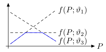
Figure 1: Pointwise minimization of a family of linear functions (dashed straight lines) results in a concave function (piecewise linear solid blue line).

Proposition 2

There exists a minimum binary solution of $E(\mathbf{P})$ under constraint (3) when $A(\mathbf{P})+\mathbf{H}\succ 0$.

Proof:We already proved that $E$ is concave when $A(\mathbf{P})+\mathbf{H}\succ 0$. It is well known that the minimum solution of a concave function over a polytope can be taken at one of its vertices. The proposition follows by combining this result with the total unimodularity of constraint (3) as stated previously.

To facilitate optimization of $E$, matrix $\mathbf{P}$ needs first to be vectorized. Let us define the vectorization of a matrix as the concatenation of its rows , denoted by $\text{vec}(\cdot)$. Let $\mathbf{p}\triangleq\text{vec}(\mathbf{P})$. To obtain a new form of $E$ which has fewer nonlinear terms, we need some new denotations. Let

$$\text{vec}\{\mathbf{J}^{\top}[\text{diag}(\mathbf{P}\mathbf{1}_{n})\otimes\mathbf{I}_{d}]\mathbf{J}\}=\text{vec}\{\mathbf{J}_{2}^{\top}[(\mathbf{P}\mathbf{1}_{n})\otimes\mathbf{I}_{n_{\theta}}]\} =\mathbf{B}\mathbf{p},$$

$$\mathbf{J}^{\top}(\mathbf{P}\otimes\mathbf{I}_{d})\mathbf{y} =\mathbf{C}\mathbf{p},$$

$$\text{vec}\{\mathbf{J}^{\top}[(\mathbf{P}\mathbf{1})\otimes\mathbf{I}_{d}]\} =\mathbf{D}\mathbf{p},$$

$$[(\mathbf{1}^{\top}\mathbf{P})\otimes\mathbf{I}_{d}]\mathbf{y} =\mathbf{F}\mathbf{p}$$

where $n_{\theta}$ denotes the dimension of ${\boldsymbol{\theta}}$ and $\mathbf{J}_{2}\triangleq\begin{bmatrix}\mathbf{J}(\mathbf{x}_{1})^{\top}\mathbf{J}(\mathbf{x}_{1}),\ldots,\mathbf{J}(\mathbf{x}_{m})^{\top}\mathbf{J}(\mathbf{x}_{m})\end{bmatrix}^{\top}$. Based on the fact $\text{vec}(\mathbf{M}_{1}\mathbf{M}_{2}\mathbf{M}_{3})=(\mathbf{M}_{1}\otimes\mathbf{M}_{3}^{\top})\text{vec}(\mathbf{M}_{2})$ for any matrices $\mathbf{M}_{1}$, $\mathbf{M}_{2}$ and $\mathbf{M}_{3}$, we have

$$\mathbf{B} =(\mathbf{J}_{2}^{\top}\otimes\mathbf{I}_{n_{\theta}})\boldsymbol{\Psi}^{m,1}_{n_{\theta}}(\mathbf{I}_{m}\otimes\mathbf{1}_{n}^{\top}),$$

$$\mathbf{C} =(\mathbf{J}^{\top}\otimes\mathbf{y}^{\top})\boldsymbol{\Psi}^{m,n}_{d},$$

$$\mathbf{D} =(\mathbf{J}^{\top}\otimes\mathbf{I}_{d})\boldsymbol{\Psi}^{m,1}_{d}(\mathbf{I}_{m}\otimes\mathbf{1}_{n}^{\top}),$$

$$\mathbf{F} =(\mathbf{I}_{d}\otimes\mathbf{y}^{\top})\boldsymbol{\Psi}^{1,n}_{d}(\mathbf{1}_{m}^{\top}\otimes\mathbf{I}_{n})$$

Here the $mnd^{2}\times mn$ matrix $\boldsymbol{\Psi}^{m,n}_{d}\triangleq\mathbf{I}_{m}\otimes\begin{bmatrix}\mathbf{I}_{n}\otimes(\mathbf{e}_{d}^{1})^{\top},\dots,\mathbf{I}_{n}\otimes(\mathbf{e}_{d}^{d})^{\top}\end{bmatrix}^{\top}$ satisfies $\text{vec}(\mathbf{M}_{m,n}\otimes\mathbf{I}_{d})=\boldsymbol{\Psi}^{m,n}_{d}\text{vec}(\mathbf{M}_{m,n})$ for any $m\times n$ matrix $\mathbf{M}_{m,n}$, where $\mathbf{e}_{d}^{i}$ denotes the $d$-dimensional column vector with the $i$-th entry being $1$ and all other entries being $0$. $\boldsymbol{\Psi}^{m,n}_{d}$ is a large but sparse matrix and can be implemented using function $speye$ in Matlab.

With the above preparation, $E$ can be written in terms of vector $\mathbf{p}$ as:

$$E(\mathbf{p})= -[b^{\top}(\mathbf{p})+\boldsymbol{\theta}_{0}^{\top}\mathbf{H}][\mathbf{A}(\mathbf{p})+\mathbf{H}]^{-1}[b(\mathbf{p})+\mathbf{H}\boldsymbol{\theta}_{0}]-\frac{1}{n_{p}}\|\mathbf{F}\mathbf{p}\|^{2}+({\mathbf{1}}^{\top}\otimes\mathbf{\widetilde{y}}^{\top})\mathbf{p}$$ (7)

where

$$\mathbf{A}(\mathbf{p})\triangleq \text{mat}(\mathbf{B}\mathbf{p})-\frac{1}{n_{p}}\text{mat}(\mathbf{D}\mathbf{p})\text{mat}^{\top}(\mathbf{D}\mathbf{p})$$

$$\mathbf{b}(\mathbf{p})\triangleq \mathbf{C}\mathbf{p}-\frac{1}{n_{p}}\text{mat}(\mathbf{D}\mathbf{p})\mathbf{F}\mathbf{p}$$

Here $\text{mat}(\cdot)$ denotes reconstructing a symmetric matrix from a vector which is the result of applying $\text{vec}(\cdot)$ to a symmetric matrix. Therefore, $\text{mat}(\cdot)$ can be seen as the inverse of operator $\text{vec}(\cdot)$ applied to a symmetric matrix and its meaning will be clear from the context.

Since $\mathbf{1}^{\top}_{mn}\mathbf{p}=n_{p}$, a constant value, regardless of the values of $\mathbf{p}$, rows in $\mathbf{B}$, $\mathbf{C}$, $\mathbf{D}$ and $\mathbf{F}$ equal to multiple of $\mathbf{1}^{\top}_{mn}$ will be useless and can be removed. It can be verified that for 2D similarity and affine transformations and 3D scaling + translation transformation (please refer to Sec. 6 for detail), $\mathbf{B}$ and $\mathbf{D}$ contains such rows. Also, redundant rows can be removed. Since $\text{mat}(\mathbf{B}\mathbf{p})$ and $\text{mat}(\mathbf{D}\mathbf{p})$ are symmetric matrices, $\mathbf{B}$ and $\mathbf{D}$ will contain redundant rows. Based on the above analysis, We hereby denote $\mathbf{B}_{2}$ (respectively $\mathbf{D}_{2}$) as the matrix formed as a result of $\mathbf{B}$ (respectively $\mathbf{D}$) removing such rows. Let the QR factorization of $\begin{bmatrix}\mathbf{B}_{2}^{\top},\mathbf{D}_{2}^{\top},\mathbf{C}^{\top},\mathbf{F}^{\top}\end{bmatrix}$ be $\mathbf{Q}\mathbf{\Gamma}=\begin{bmatrix}\mathbf{B}_{2}^{\top},\mathbf{D}_{2}^{\top},\mathbf{C}^{\top},\mathbf{F}^{\top}\end{bmatrix}$, where $\mathbf{\Gamma}$ is an upper triangular matrix and the columns of $\mathbf{Q}$ are orthogonal unity vectors. In view of the form of $E$ in (7), we can see that the nonlinear part $E_{c}$ of $E$ (i.e., all the terms except for the last term in (7)) is determined by variable $\begin{bmatrix}\mathbf{B}_{2}^{\top},\mathbf{D}_{2}^{\top},\mathbf{C}^{\top},\mathbf{F}^{\top}\end{bmatrix}^{\top}\mathbf{p}=\mathbf{\Gamma}^{\top}\mathbf{Q}^{\top}\mathbf{p}=\mathbf{\Gamma}^{\top}\mathbf{u}$, which in turn is determined by a low dimensional variable $\mathbf{u}\triangleq\mathbf{Q}^{\top}\mathbf{p}$.

The specific form of $E_{c}$ in terms of variable $\mathbf{u}$ is:

$$E_{c}(\mathbf{u})= -[\mathbf{b}^{\top}(\mathbf{u})+\boldsymbol{\theta}_{0}^{\top}\mathbf{H}][\mathbf{A}(\mathbf{u})+\mathbf{H}]^{-1}[\mathbf{b}(\mathbf{u})+\mathbf{H}\boldsymbol{\theta}_{0}]-\frac{1}{n_{p}}\|(\mathbf{\Gamma}^{\top}\mathbf{u})_{F}\|^{2}$$ (8)

where

$$\mathbf{A}(\mathbf{u})\triangleq \text{mat}[(\mathbf{\Gamma}^{\top}\mathbf{u})_{B_{2}}]-\frac{1}{n_{p}}\text{mat}[(\mathbf{\Gamma}^{\top}\mathbf{u})_{D_{2}}]\text{mat}^{\top}[(\mathbf{\Gamma}^{\top}\mathbf{u})_{D_{2}}]$$

$$\mathbf{b}(\mathbf{u})\triangleq (\mathbf{\Gamma}^{\top}\mathbf{u})_{C}-\frac{1}{n_{p}}\text{mat}[(\mathbf{\Gamma}^{\top}\mathbf{u})_{D_{2}}](\mathbf{\Gamma}^{\top}\mathbf{u})_{F}$$

Here $(\mathbf{\Gamma}^{\top}\mathbf{u})_{B_{2}}$ denotes the vector formed by the elements of vector $\mathbf{\Gamma}^{\top}\mathbf{u}$ with indices equal to row indices of the submatrix $\mathbf{B}_{2}$ in matrix $\begin{bmatrix}\mathbf{B}_{2}^{\top},\mathbf{D}_{2}^{\top},\mathbf{C}^{\top},\mathbf{F}^{\top}\end{bmatrix}^{\top}$. Vectors $(\mathbf{\Gamma}^{\top}\mathbf{u})_{D_{2}}$, $(\mathbf{\Gamma}^{\top}\mathbf{u})_{C}$ and $(\mathbf{\Gamma}^{\top}\mathbf{u})_{F}$ are similarly defined. Here we abuse the use of ’mat’ so that $\text{mat}(\mathbf{B}_{2}\mathbf{p})=\text{mat}(\mathbf{B}\mathbf{p})$ and $\text{mat}(\mathbf{D}_{2}\mathbf{p})=\text{mat}(\mathbf{D}\mathbf{p})$. The meaning will be clear from the context. Assume the numbers of rows in $\mathbf{B}_{2}$ and $\mathbf{D}_{2}$ are $n_{B_{2}}$ and $n_{D_{2}}$, respectively. Then the dimension of $\mathbf{u}$ is $n_{B_{2}}+n_{D_{2}}+n_{\theta}+d$, which is much smaller than that of $\mathbf{p}$ and also independent of the cardinalities of the two point sets. This is the key reason why our algorithm is applicable to large scale problems and scale well with problem size.

4.2 Approach two: using constraints on $\theta$

The advantage of the preceding approach is that with $\boldsymbol{\theta}$ eliminated, the subsequent optimization only involves $\mathbf{P}$ which results in good computational efficiency. The disadvantage is that by using regularization on $\boldsymbol{\theta}$ where prior information about $\boldsymbol{\theta}$ needs to be supplied, the transformation solution is biased in favor of the predefined value. In particular, the resulting point matching method is not rotation invariant. To address this problem, in this section, instead of using regularization, we will consider using constraints on $\boldsymbol{\theta}$. However, with the increasing number of constraints, the optimization problem becomes slower to solve. Therefore, we will restrict the type of transformations to be the similarity transformation whose number of constraints is small compared with other types of transformations.

To facilitate derivation of functions in the following, we need to rewrite $\widetilde{E}$ in Eq. (4) using mainly matrices instead of vectors. It is easy to verify that $\widetilde{E}$ can be rewritten as:

$$\widetilde{E}(\mathbf{P},{\boldsymbol{\theta}})= \text{tr}\{\mathbf{\Phi}^{\top}(\boldsymbol{\theta})[\text{diag}(\mathbf{P}\mathbf{1})-\frac{1}{n_{p}}\mathbf{P}\mathbf{1}\mathbf{1}^{\top}\mathbf{P}^{\top}]\mathbf{\Phi}(\boldsymbol{\theta})\}$$

$$-2\text{tr}[\mathbf{\Phi}^{\top}(\boldsymbol{\theta})(\mathbf{P}-\frac{1}{n_{p}}\mathbf{P}\mathbf{1}\mathbf{1}^{\top}\mathbf{P})\mathbf{Y}]+\mathbf{1}^{\top}\mathbf{P}\mathbf{\widetilde{y}}-\frac{1}{s}\|\mathbf{1}^{\top}\mathbf{P}\mathbf{Y}\|^{2}$$ (9)

where the matrices $\mathbf{\Phi}(\boldsymbol{\theta})=\begin{bmatrix}\boldsymbol{\phi}(\mathbf{x}_{1}|\boldsymbol{\theta}),\ldots,\boldsymbol{\phi}(\mathbf{x}_{m}|\boldsymbol{\theta})\end{bmatrix}^{\top}$ and $\mathbf{Y}=\begin{bmatrix}\mathbf{y}_{1},\ldots,\mathbf{y}_{n}\end{bmatrix}^{\top}$. $\text{tr}(\cdot)$ denotes the trace of a matrix.

With the transformation chosen as similarity: $\boldsymbol{\phi}(\mathbf{x}_{i}|\boldsymbol{\theta})=s\mathbf{R}\mathbf{x}_{i}$, where $s$ denotes scale and $\mathbf{R}$ denotes rotation matrix, we have $\mathbf{\Phi}(\boldsymbol{\theta})=s\mathbf{X}\mathbf{R}^{\top}$, where the matrix $\mathbf{X}\triangleq\begin{bmatrix}\mathbf{x}_{1},\ldots,\mathbf{x}_{m}\end{bmatrix}^{\top}$. Substituting this specification into Eq. (9), we get our energy function as:

$$E(\mathbf{P},s,\mathbf{R})=\widetilde{E}(\mathbf{P},\boldsymbol{\theta})|_{\boldsymbol{\phi}(\mathbf{x}_{i}|\boldsymbol{\theta})=s\mathbf{R}\mathbf{x}_{i}}$$

$$=s^{2}(\mathbf{\widetilde{x}}^{\top}\mathbf{P}\mathbf{1}-\frac{1}{n_{p}}\|\mathbf{X}^{\top}\mathbf{P}\mathbf{1}\|^{2})+\mathbf{1}^{\top}\mathbf{P}\mathbf{\widetilde{y}}-2s\,\text{tr}[\mathbf{R}\mathbf{X}^{\top}(\mathbf{P}-\frac{1}{n_{p}}\mathbf{P}\mathbf{1}\mathbf{1}^{\top}\mathbf{P})\mathbf{Y}]-\frac{1}{n_{p}}\|\mathbf{1}^{\top}\mathbf{P}\mathbf{Y}\|^{2}$$ (10)

where the vector $\mathbf{\widetilde{x}}\triangleq\begin{bmatrix}\|\mathbf{x}_{1}\|_{2}^{2},\dots,\|\mathbf{x}_{m}\|_{2}^{2}\end{bmatrix}^{\top}$.

It is clear that

$$\min_{\mathbf{P},s,\mathbf{R}}E(\mathbf{P},s,\mathbf{R})=\min_{\mathbf{P}}\{\min_{s,\mathbf{R}}E(\mathbf{P},s,\mathbf{R})\}=\min_{\mathbf{P}}E(\mathbf{P})$$

where the energy function

$$E(\mathbf{P})\triangleq\min_{s,\mathbf{R}}E(\mathbf{P},s,\mathbf{R})$$ (11)

Therefore, the minimization of $E(\mathbf{P},s,\mathbf{R})$ now boils down to the minimization of $E(\mathbf{P})$. $E(\mathbf{P})$ can be characterized by the following propositions:

Proposition 3

$E(\mathbf{P})$ is concave.

Proof:Based on the aforementioned derivation of the energy function, we have $\widetilde{E}(\mathbf{P},\boldsymbol{\theta})=\min_{{\mathbf{t}}}\widetilde{E}(\mathbf{P},\boldsymbol{\theta},\mathbf{t})$ and $E(\mathbf{P})=\min_{s,\mathbf{R}}\widetilde{E}(\mathbf{P},\boldsymbol{\theta})|_{\boldsymbol{\phi}(\mathbf{x}_{i}|\boldsymbol{\theta})=s\mathbf{R}\mathbf{x}_{i}}$. Therefore, we have
$E(\mathbf{P})=\min_{s,\mathbf{R},{\mathbf{t}}}\widetilde{E}(\mathbf{P},\boldsymbol{\theta},{\mathbf{t}})|_{\boldsymbol{\phi}(\mathbf{x}_{i}|\boldsymbol{\theta})=s\mathbf{R}\mathbf{x}_{i}}$. It is clear that $\widetilde{E}(\mathbf{P},\boldsymbol{\theta},{\mathbf{t}})|_{\boldsymbol{\phi}(\mathbf{x}_{i}|\boldsymbol{\theta})=s\mathbf{R}\mathbf{x}_{i}}$ is linear with respect to $\mathbf{P}$. We see that $E(\mathbf{P})$ is the result of pointwise minimization of a family of linear functions, and hence is concave, as illustrated in Fig. 1.

Proposition 4

There exists a minimum binary solution of $E(\mathbf{P})$ under constraint (3).

We omit the proof of proposition 4 as it is similar to that of proposition 2. Proposition 3 shows that $E$ is concave regardless of the values of $\mathbf{P}$, which is in contrast to the preceding approach where the energy function is only concave over a finite region.

To facilitate optimization of $E$, $E$ needs to be expressed in terms of vector $\mathbf{p}$. To obtain a new form of $E$ which has fewer nonlinear terms, we first need some denotations. Let

$$\text{vec}(\mathbf{X}^{\top}\mathbf{P}\mathbf{Y})\triangleq \mathbf{B}\mathbf{p},$$ (12)

$$\mathbf{X}^{\top}\mathbf{P}\mathbf{1}\triangleq \mathbf{C}\mathbf{p},$$ (13)

$$\mathbf{Y}^{\top}\mathbf{P}^{\top}\mathbf{1}\triangleq \mathbf{D}\mathbf{p},$$ (14)

$$\mathbf{\widetilde{x}}^{\top}\mathbf{P}\mathbf{1}\triangleq \mathbf{a}^{\top}\mathbf{p}$$ (15)

Based on the fact $\text{vec}(\mathbf{M}_{1}\mathbf{M}_{2}\mathbf{M}_{3})=(\mathbf{M}_{1}\otimes\mathbf{M}_{3}^{\top})\text{vec}(\mathbf{M}_{2})$ for any matrices $\mathbf{M}_{1}$, $\mathbf{M}_{2}$ and $\mathbf{M}_{3}$, we have

$$\mathbf{B}=\mathbf{X}^{\top}\otimes\mathbf{Y}^{\top},\mathbf{C}=\mathbf{X}^{\top}\otimes\mathbf{1}_{n}^{\top},\mathbf{D}=\mathbf{1}_{m}^{\top}\otimes\mathbf{Y}^{\top},\mathbf{a}=\mathbf{\widetilde{x}}\otimes\mathbf{1}_{n}$$

With the above preparation, $E(\mathbf{P})$ can be rewritten in terms of $\mathbf{p}$ as

$$E(\mathbf{p})= (\mathbf{1}_{m}^{\top}\otimes\mathbf{\widetilde{y}}^{\top})\mathbf{p}-\frac{1}{n_{p}}\|\mathbf{D}\mathbf{p}\|^{2}+\min_{s,\mathbf{R}}\{s^{2}(\mathbf{a}^{\top}\mathbf{p}-\frac{1}{n_{p}}\|\mathbf{C}\mathbf{p}\|^{2})$$

$$-2s\,\text{tr}(\mathbf{R}[\text{mat}(\mathbf{B}\mathbf{p})-\frac{1}{n_{p}}\mathbf{C}\mathbf{p}\mathbf{p}^{\top}\mathbf{D}^{\top}])\}$$ (16)

Let the QR factorization of matrix $\begin{bmatrix}\mathbf{B}^{\top},\mathbf{C}^{\top},\mathbf{D}^{\top},\mathbf{a}^{\top}\end{bmatrix}$ be $\mathbf{Q}\mathbf{\Gamma}=\begin{bmatrix}\mathbf{B}^{\top},\mathbf{C}^{\top},\mathbf{D}^{\top},\mathbf{a}^{\top}\end{bmatrix}$, where $\mathbf{\Gamma}$ is an upper triangular matrix and the columns of $\mathbf{Q}$ are orthogonal unity vectors. In view of the form of $E$ in (16), we can see that the nonlinear part $E_{c}$ of $E$ (i.e., all the terms except for the first term in (16)) is determined by $\begin{bmatrix}\mathbf{B}^{\top},\mathbf{C}^{\top},\mathbf{D}^{\top},\mathbf{a}^{\top}\end{bmatrix}^{\top}\mathbf{p}=\mathbf{\Gamma}^{\top}\mathbf{Q}^{\top}\mathbf{p}=\mathbf{\Gamma}^{\top}\mathbf{u}$, which in turn is determined by a low dimensional variable $\mathbf{u}\triangleq\mathbf{Q}^{\top}\mathbf{p}$. The specific form of $E_{c}$ in terms of $\mathbf{u}$ is:

$$E_{c}(\mathbf{u})= -\frac{1}{n_{p}}\|(\mathbf{\Gamma}^{\top}\mathbf{u})_{D}\|^{2}+\min_{s,\mathbf{R}}\{s^{2}((\mathbf{\Gamma}^{\top}\mathbf{u})_{a}-\frac{1}{n_{p}}\|(\mathbf{\Gamma}^{\top}\mathbf{u})_{C}\|^{2})$$

$$-2s\,\text{tr}(\mathbf{R}[\text{mat}((\mathbf{\Gamma}^{\top}\mathbf{u})_{B})-\frac{1}{n_{p}}(\mathbf{\Gamma}^{\top}\mathbf{u})_{C}(\mathbf{\Gamma}^{\top}\mathbf{u})_{D}^{\top}])\}$$ (17)

Here $(\mathbf{\Gamma}^{\top}\mathbf{u})_{B}$ denotes the vector formed by the elements of vector $\mathbf{\Gamma}^{\top}\mathbf{u}$ with indices equal to row indices of the submatrix $\mathbf{B}$ in matrix $\begin{bmatrix}\mathbf{B}^{\top},\mathbf{C}^{\top},\mathbf{D}^{\top},\mathbf{a}^{\top}\end{bmatrix}^{\top}$. Vectors $(\mathbf{\Gamma}^{\top}\mathbf{u})_{C}$, $(\mathbf{\Gamma}^{\top}\mathbf{u})_{D}$ and $(\mathbf{\Gamma}^{\top}\mathbf{u})_{a}$ are similarly defined. The dimension of $\mathbf{u}$ is $d^{2}+2d+1$, which is independent of the cardinalities of the two point sets. This is the key reason why our algorithm scales well with problem size.

4.2.1 2D case

Although the preceding energy function derivation directly applies to the 2D case, an energy function with even fewer nonlinear terms can be derived for this case. Assume the rotation angle is $\beta$, then the rotation matrix is $\mathbf{R}=\begin{bmatrix}\cos(\beta)&-\sin(\beta)\\ \sin(\beta)&\cos(\beta)\end{bmatrix}$. Let a unit vector $\mathbf{r}\triangleq[\cos(\beta),\sin(\beta)]^{\top}$, then we have

$$\text{tr}(\mathbf{R}\mathbf{H})=\mathbf{r}^{\top}\mathbf{W}\text{vec}(\mathbf{H})$$ (18)

for any $2\times 2$ matrix $\mathbf{H}$, where the constant matrix $\mathbf{W}\triangleq\begin{bmatrix}1&0&0&1\\ 0&1&-1&0\end{bmatrix}$.

Based on Eq. (18) and the fact that $\max_{\mathbf{r}}\mathbf{r}^{\top}\boldsymbol{\eta}=\|\boldsymbol{\eta}\|$ for and 2D vector $\boldsymbol{\eta}$, we can rewrite the function $E(\mathbf{P})$ in Eq. (11) as:

$$E(\mathbf{P})= \mathbf{1}^{\top}\mathbf{P}\mathbf{\widetilde{y}}-\frac{1}{n_{p}}\|\mathbf{Y}^{\top}\mathbf{P}^{\top}\mathbf{1}\|^{2}+\min_{s}\{s^{2}(\mathbf{\widetilde{x}}^{\top}\mathbf{P}\mathbf{1}-\frac{1}{n_{p}}\|\mathbf{X}^{\top}\mathbf{P}\mathbf{1}\|^{2})$$

$$-2s\|\mathbf{W}\text{vec}(\mathbf{X}^{\top}\mathbf{P}\mathbf{Y}-\frac{1}{n_{p}}\mathbf{X}^{\top}\mathbf{P}\mathbf{1}\mathbf{1}^{\top}\mathbf{P}\mathbf{Y})\|\}$$ (19)

To facilitate the optimization of $E(\mathbf{P})$, $E(\mathbf{P})$ needs to be expressed in terms of vector $\mathbf{p}$. Instead of using the matrix denotation $\mathbf{B}$ as given in Eq. (12), we let

$$\mathbf{W}\text{vec}(\mathbf{X}^{\top}\mathbf{P}\mathbf{Y})\triangleq\mathbf{\widetilde{B}}\mathbf{p}$$

Based on the fact $\text{vec}(\mathbf{M}_{1}\mathbf{M}_{2}\mathbf{M}_{3})=(\mathbf{M}_{1}\otimes\mathbf{M}_{3}^{\top})\text{vec}(\mathbf{M}_{2})$, we have matrix $\mathbf{\widetilde{B}}=\mathbf{W}(\mathbf{X}^{\top}\otimes\mathbf{Y}^{\top})$. Then, we can write $E(\mathbf{P})$ in terms of vector $\mathbf{p}$ as:

$$E(\mathbf{p})= (\mathbf{1}_{m}^{\top}\otimes\mathbf{\widetilde{y}}^{\top})\mathbf{p}-\frac{1}{n_{p}}\|\mathbf{D}\mathbf{p}\|^{2}+\min_{s}\{s^{2}(\mathbf{a}^{\top}\mathbf{p}-\frac{1}{n_{p}}\|\mathbf{C}\mathbf{p}\|^{2})$$

$$-2s\|\mathbf{\widetilde{B}}\mathbf{p}-\frac{1}{n_{p}}\mathbf{W}\text{vec}(\mathbf{C}\mathbf{p}\mathbf{p}^{\top}\mathbf{D}^{\top})\|\}$$ (20)

Let the QR factorization of matrix $\begin{bmatrix}\mathbf{\widetilde{B}}^{\top},\mathbf{C}^{\top},\mathbf{D}^{\top},\mathbf{a}^{\top}\end{bmatrix}$ be $\mathbf{Q}\mathbf{\Gamma}=\begin{bmatrix}\mathbf{\widetilde{B}}^{\top},\mathbf{C}^{\top},\mathbf{D}^{\top},\mathbf{a}^{\top}\end{bmatrix}$. In view of the form of $E$ in Eq. (20), we can see that the concave part $E_{c}$ of $E$ (i.e., all the terms except for the first term in (20)) is determined by $\begin{bmatrix}\mathbf{\widetilde{B}}^{\top},\mathbf{C}^{\top},\mathbf{D}^{\top},\mathbf{a}^{\top}\end{bmatrix}^{\top}\mathbf{p}=\mathbf{\Gamma}^{\top}\mathbf{Q}^{\top}\mathbf{p}=\mathbf{\Gamma}^{\top}\mathbf{u}$, which in turn is determined by variable $\mathbf{u}\triangleq\mathbf{Q}^{\top}\mathbf{p}$. The specific form of $E_{c}$ in terms of $\mathbf{u}$ is

$$E_{c}(\mathbf{u})= -\frac{1}{n_{p}}\|(\mathbf{\Gamma}^{\top}\mathbf{u})_{D}\|^{2}+\min_{s}\{s^{2}[(\mathbf{\Gamma}^{\top}\mathbf{u})_{a}-\frac{1}{n_{p}}\|(\mathbf{\Gamma}^{\top}\mathbf{u})_{C}\|^{2}]$$

$$-2s\|(\mathbf{\Gamma}^{\top}\mathbf{u})_{\widetilde{B}}-\frac{1}{n_{p}}\mathbf{W}\text{vec}((\mathbf{\Gamma}^{\top}\mathbf{u})_{C}(\mathbf{\Gamma}^{\top}\mathbf{u})_{D}^{\top})\|\}$$ (21)

Here the vector $(\mathbf{\Gamma}^{\top}\mathbf{u})_{\widetilde{B}}$ is similarly defined as vectors $(\mathbf{\Gamma}^{\top}\mathbf{u})_{C}$, $(\mathbf{\Gamma}^{\top}\mathbf{u})_{D}$ and $(\mathbf{\Gamma}^{\top}\mathbf{u})_{a}$.

It is easy to verify that the dimension of $\mathbf{u}$ is $3d+1|_{d=2}=7$, which is lower than the dimension $d^{2}+2d+1|_{d=2}=9$ as a result of directly applying the energy function derivation prior to this subsection to the 2D case.

5 Optimization

Our analysis in the previous section indicates that the nonlinear part of $E(\mathbf{p})$ is determined by a low dimensional variable $\mathbf{u}$ and is also concave. Therefore it is natural to use the normal simplicial algorithm [13], a BnB algorithm specifically designed for concave functions, to optimize $E$.

5.1 Initial enclosing region

In the normal simplicial algorithm, simplexes are used to construct the convex envelopes of a concave function. Therefore the initial enclosing region should be chosen as a simplex or a collection of simplexes. We use a collection of simplexes to enclose the feasible region $U\triangleq\{\mathbf{u}|\mathbf{u}=\mathbf{Q}^{\top}\mathbf{p},\mathbf{p}\in\Omega\}$ as the resulting enclosing could be more tight, where $\Omega$ denotes the feasible region of $\mathbf{p}$, as determined by (3). The procedure is as follows. We first choose an interior point $\mathbf{v}_{0}=\mathbf{Q}^{\top}\frac{n_{p}}{mn}\mathbf{1}_{mn}$ of $U$, which corresponds to the fuzziest point correspondence. We then construct a new coordinate system by translating the coordinate system of $\mathbf{u}$ so that the new origin locates at $\mathbf{v}_{0}$, as illustrated in Fig. 2. We now construct each enclosing simplex as the intersection of an orthant of the new coordinate system with a half space containing $U$, whose face supports $U$ and has a normal vector $\mathbf{h}$ chosen as the normalized mean of the orthant axes, as illustrated in Fig. 2.

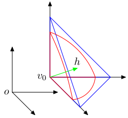
Figure 2: Red region: the intersection of $U$ with an orthant of the new coordinate system. Blue region: an enclosing simplex, one of whose faces supports $U$ and has a normal $\mathbf{h}$ (in green) equal to the normalized mean of the orthant axes.

The distance from $\mathbf{v}_{0}$ to the supporting plane with normal $\mathbf{h}$ can be computed as:

$$\max\{\mathbf{h}^{\top}(\mathbf{Q}^{\top}\mathbf{p}-\mathbf{v}_{0})|\mathbf{p}\in\Omega\}$$ (22)

This is a k-cardinality linear assignment problem which can be either directly solved [1] or transformed into a standard linear assignment problem [32] (we adopt the latter approach and choose the Jonker-Volgenant algorithm [16] for the resulting problem in this paper). The supporting plane with normal $\mathbf{h}$ can then be completely determined. In turn, the vertices of the enclosing simplex can be recovered which has $\mathbf{v}_{0}$ as one of its vertices.

5.2 Choice of $\mathbf{H}$ in approach one of our algorithm

For approach one of our algorithm, we need to ensure $E$ is concave over all the enclosing simplexes. Based on proposition 1, it suffices if $\mathbf{A}(\mathbf{u})+\mathbf{H}\succ 0$ for any $\mathbf{u}$ belonging to the enclosing simplexes. This condition can be satisfied by setting the eigenvalues of $\mathbf{H}$ to be large enough. The procedure is as follows. Assume the eigenvalues of $\mathbf{A}(\mathbf{v}_{i})$ are $\lambda^{j}_{i}$, where $\mathbf{v}_{i}$ is a vertex of the enclosing simplexes. We choose a scalar $\lambda_{0}=\min\{\min_{i,j}{\lambda_{i}^{j}},0\}$ and set $\mathbf{H}=(-\lambda_{0}+\epsilon_{0})\mathbf{I}$, where $\epsilon_{0}$ is a small positive value (we set $\epsilon_{0}=10^{-5}$ in this paper). We now have $\mathbf{A}(\mathbf{v}_{i})+\mathbf{H}\succ 0$ for any vertex $\mathbf{v}_{i}$ of the enclosing simplexes. Since $\mathbf{A}(\mathbf{u})+\mathbf{H}\succ 0$ is a spectrahedra and thus convex as indicated by proposition 1, we therefore have $\mathbf{A}(\mathbf{u})+\mathbf{H}\succ 0$ for any $\mathbf{u}$ belonging to the enclosing simplexes.

5.3 Lower bounds

The convex envelope $E_{cs}$ of the concave part $E_{c}(\mathbf{u})$ of $E$ over a simplex $S=[\mathbf{v}_{1},\ldots,\mathbf{v}_{n_{u}+1}]$ is the unique affine function which coincides with $E_{c}$ at the vertices $\mathbf{v}_{1},\ldots,\mathbf{v}_{n_{u}+1}$ [13], i.e., $E_{cs}(\mathbf{u})=\sum_{i=1}^{n_{u}+1}\alpha_{i}E_{c}(\mathbf{v}_{i})$ with $\mathbf{u}=\sum_{i=1}^{n_{u}+1}\alpha_{i}\mathbf{v}_{i}$, $\sum_{i=1}^{n_{u}+1}\alpha_{i}=1$, $\alpha_{i}\geq 0$, $\forall i$. Here $n_{u}$ denotes the dimension of $\mathbf{u}$. Based on this result, the lower bound of $E$ for region $\Omega\cap S$ can be obtained as the optimal value of the following linear program:

$$\min_{\alpha_{i},\mathbf{p}}\ \sum_{i=1}^{n_{u}+1}\alpha_{i}E_{c}(\mathbf{v}_{i})+(\mathbf{1}_{m}^{\top}\otimes\mathbf{\widetilde{y}}^{\top})\mathbf{p}$$

$$s.t.\sum_{i=1}^{n_{u}+1}\alpha_{i}\mathbf{v}_{i}=\mathbf{Q}^{\top}\mathbf{p},\sum_{i=1}^{n_{u}+1}\alpha_{i}=1,\alpha_{i}\geq 0,\forall i,\mathbf{p}\in\Omega$$ (23)

By tweaking this linear program, in Sec. 5.6, we will propose an alternative lower bounding problem which is much more efficient to solve.

5.3.1 Value of $E(\mathbf{v}_{i})$ in approach two of our algorithm

For approach two of our algorithm, the value of $E(\mathbf{v}_{i})$ needs to be determined. In 3D case, $E(\mathbf{v}_{i})$ has the following form:

$$E(\mathbf{v}_{i})= -\frac{1}{n_{p}}\|(\mathbf{\Gamma}^{\top}\mathbf{v}_{i})_{D}\|^{2}+\min_{s,\mathbf{R}}\{s^{2}[(\mathbf{\Gamma}^{\top}\mathbf{v}_{i})_{a}-\frac{1}{n_{p}}\|(\mathbf{\Gamma}^{\top}\mathbf{v}_{i})_{C}\|^{2}]$$

$$-2s\,\text{tr}(\mathbf{R}[\text{mat}((\mathbf{\Gamma}^{\top}\mathbf{v}_{i})_{B})-\frac{1}{n_{p}}(\mathbf{\Gamma}^{\top}\mathbf{v}_{i})_{C}(\mathbf{\Gamma}^{\top}\mathbf{v}_{i})_{D}^{\top}])\}$$ (24)

Let matrix

$$\mathbf{G}\triangleq\text{mat}((\mathbf{\Gamma}^{\top}\mathbf{v}_{i})_{B})-\frac{1}{n_{p}}(\mathbf{\Gamma}^{\top}\mathbf{v}_{i})_{C}(\mathbf{\Gamma}^{\top}\mathbf{v}_{i})_{D}^{\top}$$

and let $\mathbf{U}\mathbf{S}\mathbf{V}^{\top}$ be the singular value decomposition of $\mathbf{G}^{\top}$, where $\mathbf{S}$ is a diagonal matrix and the columns of $\mathbf{U}$ and $\mathbf{V}$ are orthogonal unity vectors. Then the optimal rotation matrix $\mathbf{R}$ solving problem (24) is $\mathbf{R}^{*}=\mathbf{U}\text{diag}(\begin{bmatrix}1,\ldots,1,\det(\mathbf{U}\mathbf{V}^{\top})\end{bmatrix})\mathbf{V}^{\top}$ [25]. Here $\text{diag}(\cdot)$ denotes converting a vector into a diagonal matrix, and $\det(\cdot)$ denotes the determinant of a square matrix. By substituting $\mathbf{R}^{*}$ back into (24), $\mathbf{R}$ is eliminated and we get a (possibly concave) quadratic program only in one variable $s$. If the range of $s$ is $\underline{s}\leq s\leq\overline{s}$, then one can easily solve this quadratic program by comparing the function values at the two boundary points $\underline{s}$, $\overline{s}$ and the extreme point to obtain the optimal $s$.

2D case: For 2D case, we have

$$E(\mathbf{v}_{i})= -\frac{1}{n_{p}}\|(\mathbf{\Gamma}^{\top}\mathbf{v}_{i})_{D}\|^{2}+\min_{s}\{s^{2}((\mathbf{\Gamma}^{\top}\mathbf{v}_{i})_{a}-\frac{1}{n_{p}}\|(\mathbf{\Gamma}^{\top}\mathbf{v}_{i})_{C}\|^{2})$$

$$-2s\|(\mathbf{\Gamma}^{\top}\mathbf{v}_{i})_{B_{2}}-\frac{1}{n_{p}}\mathbf{W}\text{vec}((\mathbf{\Gamma}^{\top}\mathbf{v}_{i})_{C}(\mathbf{\Gamma}^{\top}\mathbf{v}_{i})_{D}^{\top})\|\}$$ (25)

This is a quadratic program in only one variable $s$. Hence the optimal $s$ can similarly be solved based on the above discussion.

5.4 Division of a simplex

Since the BnB algorithm is used for optimization, during the branching phase, a chosen simplex needs to be subdivided into several smaller simplexes. We adopt the following simple strategy to divide a simplex. For a chosen simplex, the longest edge is bisected. This results in two sub-simplexes. It has been proved that such a subdivision scheme leads to a BnB algorithm that converges [13].

5.5 The normal simplicial BnB algorithm

With the preparation from the previous subsections, We are now ready to describe the algorithm for minimizing $E(\mathbf{p})$. During initialization, a set of simplexes whose union contains the feasible region $\Omega$ is computed. Then in each iteration, the simplex yielding the lowest lower bound among all the simplexes is further subdivided so as to improve the lower bound of $E$ for $\Omega$. Meanwhile, the upper bound is updated by evaluating $E$ with solutions of the linear programs used to compute the lower bounds. The pseudo-code of the algorithm is summarized in Algorithm 1.

1

2Initialization

3Select tolerance error $\epsilon>0$.

4Find a collection of simplexes $\{S_{i}\}$ such that $U\subset{\cup_{i}}S_{i}$ according to Sec. 5.1. (For approach one, choose $\mathbf{H}$ according to Sec. 5.2.) Set $\mathscr{M}_{1}=\mathscr{N}_{1}=\{S_{i}\}$, where $\mathscr{M}_{1}$ denotes the collection of all simplexes and $\mathscr{N}_{1}$ denotes the collection of active simplexes.

5for $k=1,2,\ldots$ do

6      

7      For each simplex $S\in\mathscr{N}_{k}$, solve the linear program (23) to obtain a basic optimal solution $\boldsymbol{\omega}(S)$ and the optimal value $\beta(S)$. $\beta(S)$ is the lower bound of $E$ for region $\Omega\cap S$.

8      Let $\mathbf{p}^{k}$ equal the best among all feasible solutions so far encountered: $\mathbf{p}^{k-1}$ and all $\boldsymbol{\omega}(S),S\in\mathscr{N}_{k}$. Delete all simplexes $S\in\mathscr{M}_{k}$ such that $\beta(S)\geq E(\mathbf{p}^{k})-\epsilon$. Let $\mathscr{R}_{k}$ be the remaining collection of simplexes.

9      If $\mathscr{R}_{k}=\emptyset$, terminate: $\mathbf{p}^{k}$ is the global $\epsilon$-minimal solution. Otherwise, go to the next step.

10      Select the simplex to be divided: $S_{k}\in\arg\min\{\beta(S)|S\in\mathscr{R}_{k}\}$.

11      Divide $S_{k}$ according to Sec. 5.4 to get two sub-simplexes $S_{k1}$ and $S_{k2}$.

12      Let $\mathscr{N}_{k+1}=\{S_{k1},S_{k2}\}$ and $\mathscr{M}_{k+1}=(\mathscr{R}_{k}\backslash\{S_{k}\})\cup\mathscr{N}_{k+1}$.

13 end for

14

Algorithm 1 The normal simplicial algorithm for minimizing $E$

5.6 A new fast lower bounding scheme

Our algorithm is an instance of the BnB technique, therefore it contains three basic subroutines: branching, finding upper and lower bounds. It is obvious that the lower bounding subroutine (23) requires much more time to compute than the other two subroutines since it is a generic linear program, for which there are no efficient algorithms. To address this problem, in this subsection, we will propose an alternative lower bounding scheme which is more efficient to compute.

To this end, a natural idea is to drop the inequality constraints $\alpha_{i}\geq 0,\forall i$ in (23), then there are only linear equality constraints on $\alpha_{i}$. Therefore $\alpha_{i}$ can be eliminated via algebraic substitution and we arrive at the following equivalent problem:

$$\min E_{S}(\mathbf{p})= ([E_{c}(\mathbf{v}_{1}),\ldots,E_{c}(\mathbf{v}_{n_{u}})]-E_{c}(\mathbf{v}_{n_{u}+1})\mathbf{1}_{n_{u}}^{\top})([\mathbf{v}_{1},\ldots,\mathbf{v}_{n_{u}}]-\mathbf{v}_{n_{u}+1}\mathbf{1}_{n_{u}}^{\top})^{-1}(\mathbf{Q}^{\top}\mathbf{p}-\mathbf{v}_{n_{u}+1})$$

$$+E_{c}(\mathbf{v}_{n_{u}+1})+(\mathbf{1}_{m}^{\top}\otimes\mathbf{\widetilde{y}}^{\top})\mathbf{p}$$

$$s.t.\quad\mathbf{p}\in\Omega$$ (26)

Problem (26) is a k-cardinality linear assignment problem which can be efficiently solved by the combinatorial optimization algorithms mentioned in Sec. 5.1. Note that simplex $S$ will not degenerate throughout the BnB iterations and therefore matrix $[\mathbf{v}_{1},\ldots,\mathbf{v}_{n_{u}}]-\mathbf{v}_{n_{u}+1}\mathbf{1}_{n_{u}}^{\top}$ is always invertible. We have the following proposition.

Proposition 5

The optimal value of problem (26) is a lower bound of $E$ for region $\Omega\cap S$.

Proof:Problem (26) is a relaxed version of (23) by dropping the constraints $\alpha_{i}\geq 0,\forall i$. Therefore the optimal value of (26) will not be greater than that of (23), whereas solving (23) yields a lower bound of $E$ for region $\Omega\cap S$.

What remains is to check whether the lower bound computed by (26) is close to the original lower bound. In iteration $k$ of our algorithm, the lowest one among all the lower bounds corresponding to simplexes in $\mathscr{M}_{k}$ is chosen as the lower bound of $E$ for the feasible region $\Omega$. Therefore only the lowest lower bound determines the quality of a bounding scheme. Without loss of generality, let us assume that $\widetilde{S}$ is the simplex yielding the lowest lower bound when using (26) to compute the lower bound of $E$ for region $\Omega$. It’s apparent that there are two possibilities for the location of the optimal solution $\mathbf{p}^{*}$ of problem (26): either $\mathbf{p}^{*}\in\{\mathbf{p}|E_{\widetilde{S}}(\mathbf{p})\leq E(\mathbf{p})\}$ or $\mathbf{p}^{*}\in\{\mathbf{p}|E_{\widetilde{S}}(\mathbf{p})>E(\mathbf{p})\}$, as illustrated in Fig. 3. Note that the latter case is impossible since in this case, $E_{\widetilde{S}}(\mathbf{p}^{*})$ will be strictly larger than the minimum value of $E$ over $\Omega$, violating the assumption that $E_{\widetilde{S}}(\mathbf{p}^{*})$ is a lower bound of $E$ for region $\Omega$. Therefore it can only happen that $\mathbf{p}^{*}\in\{\mathbf{p}|E_{\widetilde{S}}(\mathbf{p})\leq E(\mathbf{p})\}$. Since $p^{*}$ can only be obtained at one of the vertices of $\Omega$. This also indicates that $\{\mathbf{p}|E_{\widetilde{S}}(\mathbf{p})\leq E(\mathbf{p})\}$ contains a segment of the boundary of $\Omega$.

From Fig. 3, we can see that $\{\mathbf{p}|E_{\widetilde{S}}(\mathbf{p})\leq E(\mathbf{p})\}$ is an ellipsoid-like region containing and circumscribing the simplex $\widetilde{S}$. Therefore, under the condition that the gradient of the plane $E_{\widetilde{S}}$ is not large, the lower bounds computed via (23) and via (26) will be close to each other.

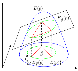
Figure 3: Ellipse-like closed curve $\{\mathbf{p}|E_{\widetilde{S}}(\mathbf{p})=E(\mathbf{p})\}$ separates the solution space into two disjoint regions. Simplex $\widetilde{S}$ is contained in the region $\{\mathbf{p}|E_{\widetilde{S}}(\mathbf{p})\leq E(\mathbf{p})\}$.

5.6.1 Effectiveness of the fast bounding scheme

In this subsection, we will compare the performances of our algorithm under either the original bounding scheme or the fast bounding scheme. We first use the outlier test as described in section 6.1.1 (which tests our first algorithm using regularization on transformation parameters) for comparison where the outlier to data ratio is chosen as $0.5$.

The lower and upper bounds for the feasible region generated by the two bounding schemes in each iteration of our algorithm are shown in figure 4. It can be seen that the difference between the lower bounds generated by the two bounding schemes widens as the number of iterations increases. The main reason is that the gradient of the energy function $E$ is large at the boundary of the feasible region of $\mathbf{u}$ (since $\mathbf{H}$ is chosen so that $\mathbf{A}(\mathbf{u})+\mathbf{H}$ is barely positive definite within the feasible region of $\mathbf{u}$, the value of $E$ (which contains inversion of $\mathbf{A}(\mathbf{u})+\mathbf{H}$) will change dramatically at the boundary of the feasible region of $\mathbf{u}$). Consequently, the gradient of the lower bounding plane $E_{\widetilde{S}}$ is also large (particularly when the simplex ${\widetilde{S}}$ becomes small) since $\{\mathbf{p}|E_{\widetilde{S}}(\mathbf{p})\leq E(\mathbf{p})\}$ contains a segment of the boundary of the feasible region of $\mathbf{u}$. As a result, the minimum value of $E_{\widetilde{S}}$ calculated within the simplex ${\widetilde{S}}$ (which is the lower bound by the original scheme) will differ significantly from the minimum value of $E_{\widetilde{S}}$ calculated within the ellipsoid-like region $\{\mathbf{p}|E_{\widetilde{S}}(\mathbf{p})\leq E(\mathbf{p})\}$ (which is the lower bound by the fast scheme). Nevertheless, from the right column of figure 4, one can see that the upper bound generated by the fast bounding scheme is always lower than that generated by the original scheme, whereas the solution of the algorithm is chosen based on the upper bound. Therefore, this indicates that the proposed fast bounding scheme is better at locating good solutions than the original scheme. Figure 4 also suggests that for fast bounding scheme, since the difference between upper and lower bounds never shrinks to zero, we cannot use the difference between the upper and lower bounds (i.e., tolerance error) to determine when to terminate our algorithm. Instead, in this paper, we will use the maximum search depth (chosen as 15) of the BnB algorithm as the termination criterion. However, this decision will causes our algorithm not to be $\epsilon-$globally optimal. Nevertheless, we empirically found that our method with this decision performs very well in practice.

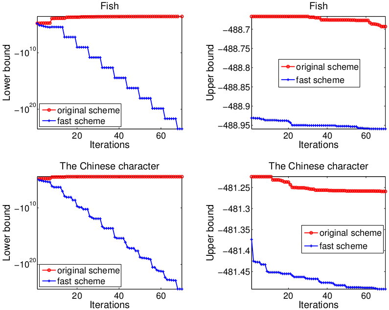
Figure 4: Mean of the lower bounds (left column) and upper bounds (right column) for the feasible region by the two bounding schemes in each iteration of our algorithm. The outlier test in section 6.1.1 is used and 2D similarity transformation is chosen for our algorithm.

The average run time of our algorithm under different choices of bounding schemes are listed in Table 1. It can be seen that the speed of our algorithm using the fast bounding scheme is $254$ times that using the original bounding scheme, demonstrating its high computational efficiency.

Table 1: Average run time of our algorithm under different choices of bounding schemes (in seconds).

	fish	the Chinese character
original scheme	722.5290	1061.5
fast scheme	2.7529	4.2801

We then use the outlier test as described in section 6.2.1 (which tests our second algorithm using constraints on transformation parameters) for comparison, where the outlier to data ratio is chosen as $0.5$.

The lower and upper bounds for the feasible region by the two schemes in each iteration of our algorithm are shown in figure 5. It can be seen that the difference between the lower bounds generated by the two bounding schemes widens as the number of iterations increases, albeit not as quickly as in the previous test. Similar reason as in the previous test can be said about this phenomenon.

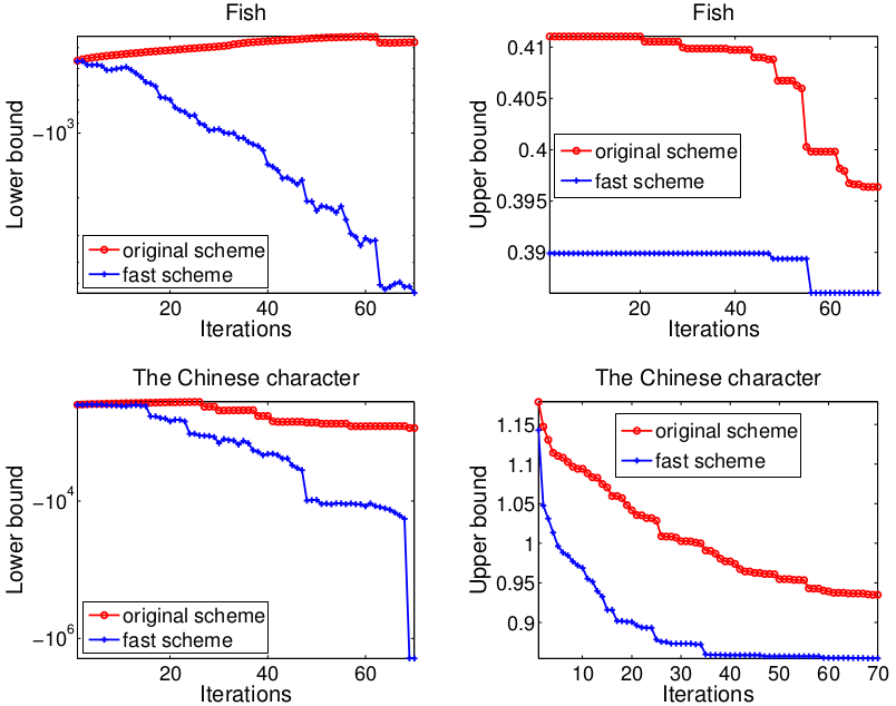
Figure 5: Mean of the lower bounds (left column) and upper bounds (right column) for the feasible region by the two bounding schemes in each iteration of our algorithm. The outlier test in section 6.2.1 is used and 2D similarity transformation is chosen for our algorithm.

5.7 GPU speed-up

Our algorithm initially needs to compute $2^{n_{u}}$ enclosing simplexes (see section 5.1) which corresponds to $2^{n_{u}}$ orthants of the space of $\mathbf{u}$ by solving the linear assignment problem (22). Then, in step 5 of algorithm 1, the linear assignment problem (26) needed to be solved for a set $\mathscr{N}_{k}$ of simplexes. Initially, the size of $\mathscr{N}_{1}$ is $2^{n_{u}}$. When $n_{u}$ is large (e.g., in the case of 3D similarity registration), the above routines cost considerable amount of time. Therefore, it’s desirable that the above routines can be computed as fast as possible. Fortunately, note that the above routines are independent repetitive routines, Therefore, it’s ideal for them to be implemented in parallel. In this paper, we implement the above routines by using the parallel programming toolbox provided by Matlab on an Nvidia Quadro K2200 GPU card. Our experimental results show that doing so can bring about 4x speed-up improvement compared with pure CPU implementation.

6 Experimental results

We implement our method under the Matlab 2014a environment and compare it with other methods on a PC with 2.4 GHz CPU and 8G RAM. For the methods to be compared which only output point correspondences, we use the correspondences generated by the methods to find the best affine transformations between two point sets. We define error as mean of the Euclidean distances between the transformed ground truth model inliers and their corresponding scene inliers.

Since there are two versions of our algorithm which have different requirements on values of transformation parameters, accordingly, we will conduct different experiments to respectively test their performances.

6.1 Experiments on point sets with no rotation between them

In this subsection, we will test our first algorithm which uses regularization on transformation and thus does not allow arbitrary rotation between two point sets. We compare it with RPM [9], CPD [25] and MG [14], whose source codes are freely available. These methods represent state-of-the-arts, only utilize the point position information for matching, and are capable of handling partial overlaps between two point sets.

6.1.1 2D synthesized datasets

Two choices of transformations are considered for our method: 2D similarity and affine transformations. For 2D similarity transformation, we let ${\boldsymbol{\theta}}=\begin{bmatrix}\theta_{1},\ldots,\theta_{4}\end{bmatrix}^{\top}$. Here $[\theta_{3},\theta_{4}]^{\top}$ represents translation and $\theta_{1}=r\cos(\beta)$ and $\theta_{2}=r\sin(\beta)$, with $r$ denoting scale and $\beta$ denoting rotation angle. Then we have the Jacobian matrix $\mathbf{J}(\mathbf{x}_{i})=\begin{bmatrix}x_{i}^{1}&-x_{i}^{2}&1&0\\ x_{i}^{2}&x_{i}^{1}&0&1\end{bmatrix}$. It can be verified that the rows of $\mathbf{B}_{2}=\mathbf{B}(1,:)$ and $\mathbf{D}_{2}=\mathbf{D}([1,2],:)$ constitute the unique rows of $\mathbf{B}$ and $\mathbf{D}$ not equal to multiple of $\mathbf{1}_{mn}^{\top}$, respectively.

For 2D affine transformation, we let ${\boldsymbol{\theta}}=\begin{bmatrix}\theta_{1},\ldots,\theta_{6}\end{bmatrix}^{\top}$ with $[\theta_{1},\ldots,\theta_{4}]^{\top}$ being the parameters of the linear part of the transformation and $[\theta_{5},\theta_{6}]^{\top}$ representing translation. Then we have $\mathbf{J}(\mathbf{x}_{i})=\begin{bmatrix}x_{i}^{1}&x_{i}^{2}&0&0&1&0\\ 0&0&x_{i}^{1}&x_{i}^{2}&0&1\end{bmatrix}$. It can be verified that the rows of $\mathbf{B}_{2}=\mathbf{B}([1,2,6],:)$ and $\mathbf{D}_{2}=\mathbf{D}([1,3],:)$ constitute the unique rows of $\mathbf{B}$ and $\mathbf{D}$ not equal to multiple of $\mathbf{1}_{mn}^{\top}$, respectively.

Affine transformation is used for RPM and rigid transformation is used for CPD and MG (other types of transformations are found to be far less robust for the types of experiments conducted in this paper).

Two categories of tests are used to evaluate performances of different methods: 1) Outlier test. Equal number of normally distributed random outliers are added to different sides of the prototype shape to generate two point sets so as to simulate outlier disturbance, as illustrated in columns 2, 3 of Fig. 6. 2) Occlusion + Outlier test. First, equal degree of occlusions are applied to the prototype shape to generate two point sets, respectively. We simulate occlusion by first finding the shortest Hamiltonian circle of the prototype point set (via solving a traveling salesman problem) and then retaining a segment of the circle starting at a random point. Then, a fixed number of normally distributed random outliers (outlier to data ratio is fixed to 0.5) are added to different sides of the two point sets so as to simulate outlier disturbance, as illustrated in columns 4, 5 of Fig. 6. For all the above tests, random scaling within range from $0.5$ to $1.5$ is applied to the prototype shape when generating the model point set and a moderate amount of nonrigid deformation is applied to the prototype shape when generating the scene point set. Two shapes [9], a fish and a character, as shown in the left column of Fig. 6, are used as the prototype shape, respectively.

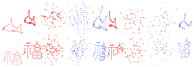
Figure 6: Left column: the prototype shapes. For the remaining columns: examples of model and scene point sets in the outlier (columns 2, 3) and occlusion + outlier (columns 4, 5) tests.

The average matching errors of different methods are shown in Fig. 7. It can be seen that our method performs much better than other methods, particularly in the occlusion+outlier test where there is a large margin between the errors of our method and those of other methods. This demonstrates our method’s robustness to disturbances. Among the different transformation choices of our method, our method using affine transformation performs relatively better than our method using similarity transformation. Among the different $n_{p}$ choices of our method, our method with $n_{p}$ chosen close to the ground truth value performs relatively better than our method with $n_{p}$ chosen far away from the ground truth value. Examples of matching results by different methods are shown in Fig. 8.

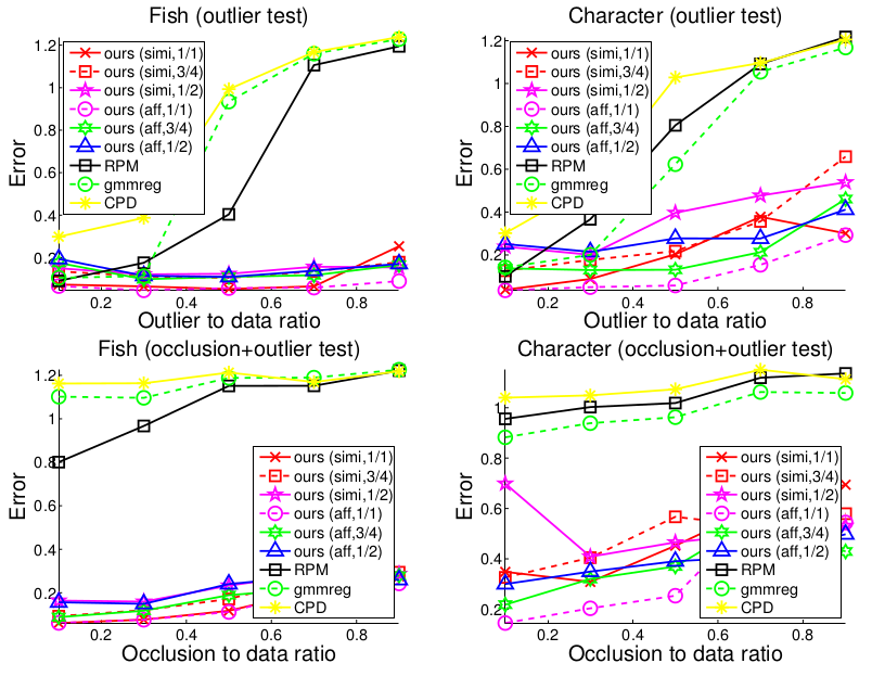
Figure 7: Average matching errors by our method under different transformation choices (similarity and affine) and with different $n_{p}$ values (chosen from $1/2$ to $1/1$ the ground truth value) and other methods over 100 random trials for the 2D outlier and occlusion+outlier tests.

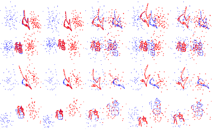
Figure 8: Examples of matching results by different methods in the outlier (top 2 rows) and occlusion + outlier (bottom 2 rows) tests.

The average running times of our method using similarity or affine transformations, RPM, gmmreg and CPD are 3.3286, 26.6627, 1.8421, 0.0613 and 0.0623 seconds, respectively. It can be seen that our method using similarity transformation has similar running time as RPM. Among the different transformation choices of our method, our method using similarity transformation is almost an order-of-magnitude faster than our method using affine transformation. This is because affine transformation have more parameters than similarity transformation, which results in a higher dimensional search space in our method and thus the BnB algorithm needs more time to converge.

6.1.2 3D synthesized datasets

Since 3D affine transformation contains too many parameters which causes our method to converge too slowly, this transformation will not be tested for our method. Instead, we consider a 3D transformation consisting of nonuniform scaling and translation for our method: $T(\mathbf{x}_{i}|\boldsymbol{\theta})=\begin{bmatrix}\theta_{1}x_{i}^{1}+\theta_{4},&\theta_{2}x_{i}^{2}+\theta_{5},&\theta_{3}x_{i}^{3}+\theta_{6}\end{bmatrix}^{\top}$ with $\boldsymbol{\theta}=[\theta_{1},\ldots,\theta_{6}]$. We have the Jacobian matrix $\mathbf{J}(\mathbf{x}_{i})=\begin{bmatrix}x_{i}^{1}&0&0&1&0&0\\ 0&x_{i}^{2}&0&0&1&0\\ 0&0&x_{i}^{3}&0&0&1\end{bmatrix}$. It can be verified that the rows of $\mathbf{B}_{2}=\mathbf{B}([1,5,9],:)$ and $\mathbf{D}_{2}=\mathbf{D}([1,5,9],:)$ constitute the unique rows of $\mathbf{B}$ and $\mathbf{D}$ not equal to multiple of $\mathbf{1}_{mn}^{\top}$, respectively.

Analogous to the experimental setup in the preceding subsection, we use two categories of tests to evaluate performances of different methods: 1) Outlier test and 2) Occlusion + Outlier test, as illustrated in Fig. 9. Two shapes, a horse and a dinosaur, as shown in the left column of Fig. 9, are used as the prototype shape, respectively.

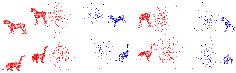
Figure 9: Left column: the prototype shapes. For the remaining columns: examples of model and scene point sets in the outlier (columns 2, 3) and occlusion+outlier (columns 4, 5) tests.

To make a fair comparison, the same 3D transformation of nonuniform scaling + translation is employed by all the comparison methods. The average matching errors of different methods are shown in Fig. 10. It can be seen that our method performs much better than other methods and its errors keep almost unchanged with the increase of severity of disturbances. This demonstrates our method’s strong robustness to disturbances. Examples of matching results by different methods are shown in Fig. 17.

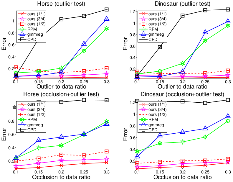
Figure 10: Average matching errors by our method with different $n_{p}$ values (chosen from $1/2$ to $1/1$ the ground truth value) and other methods over 100 random trials for the 3D outlier and occlusion+outlier tests.

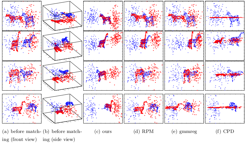
Figure 11: Examples of matching results by different methods in the outlier (top 2 rows) and occlusion+outlier (bottom 2 rows) tests.

The average running times of our method, RPM, gmmreg and CPD are 19.8839, 2.5296, 0.2842 and 0.0957 seconds, respectively.

6.2 Experiments on point sets with random rotations between them

In this subsection, we will test our second algorithm which uses constraints on transformation and allows arbitrary rotation and uniform scaling within a range between two point sets. We compare it with Go-ICP [34] which is globally optimal, only utilizes point position information and allows arbitrary rotations between two point sets. The source code of Go-ICP is generously provided by the author. The range of scale $s$ in our method is set as $0.5\leq s\leq 1.5$.

6.2.1 2D synthesized datasets

Analogous to the experimental setup in subsection 6.1.1, we use two categories of tests to evaluate performances of different methods: 1) Outlier test and 2) Occlusion + Outlier test, as illustrated in Fig. 12. Different from subsection 6.1.1, however, random rotation and scaling within range from $0.5$ to $1.5$ is also applied when generating the model point sets so as to test a method’s ability to cope with arbitrary similarity transformations.

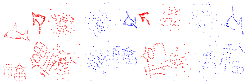
Figure 12: Left column: the prototype shapes. For the remaining columns: examples of model and scene point sets in the outlier (columns 2, 3) and occlusion + outlier (columns 4, 5) tests.

The average matching errors of our method and Go-ICP are shown in Fig. 13. It can be seen that our method performs much better than Go-ICP, especially for the occlusion+outlier test, where there is a large margin between the errors of the two methods. This demonstrates robustness of our method to disturbances.

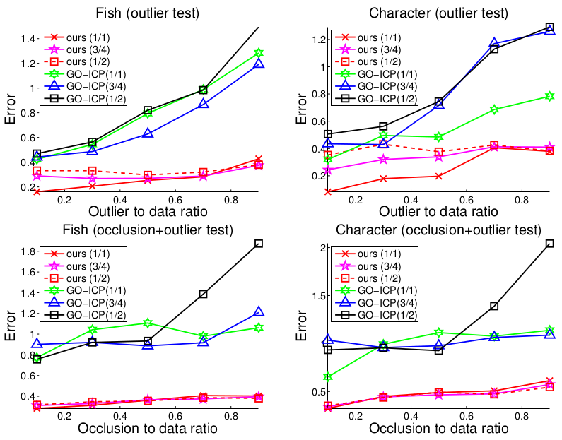
Figure 13: Average matching errors by our method and Go-ICP with different $n_{p}$ values (chosen from $1/2$ to $1/1$ the ground truth value) over 100 random trials for the 2D outlier and occlusion+outlier tests.

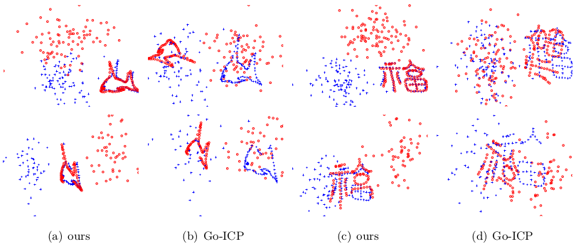
Figure 14: Examples of matching results by our method and Go-ICP for the 2D outlier (top row) and occlusion+outlier (bottom row) tests.

The average running times of our method and Go-ICP are 1.3976 and 1.1701 seconds, respectively.

6.2.2 3D synthesized datasets

Analogous to the experimental setup in the previous subsection, we use two categories of tests to evaluate performances of different methods: 1) Outlier test and 2) Occlusion + Outlier test, as illustrated in Fig. 15. The same two 3D prototype shapes as used in subsection 6.1.2 are used as the prototype shape, respectively.

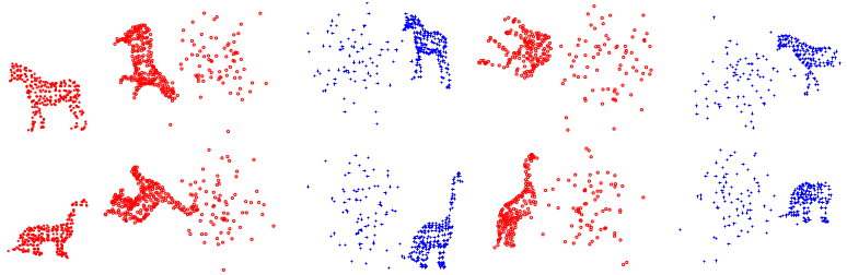
Figure 15: Left column: the prototype shapes. For the rest columns: examples of model and scene point sets in the outlier (columns 2, 3) and occlusion + outlier (columns 4, 5) tests.

The average matching errors of our method and Go-ICP are shown in Fig. 16. It can be seen that our method performs much better than Go-ICP, especially for the occlusion+outlier test, where there is a large margin between the errors of the two methods. This demonstrates robustness of our method to disturbances.

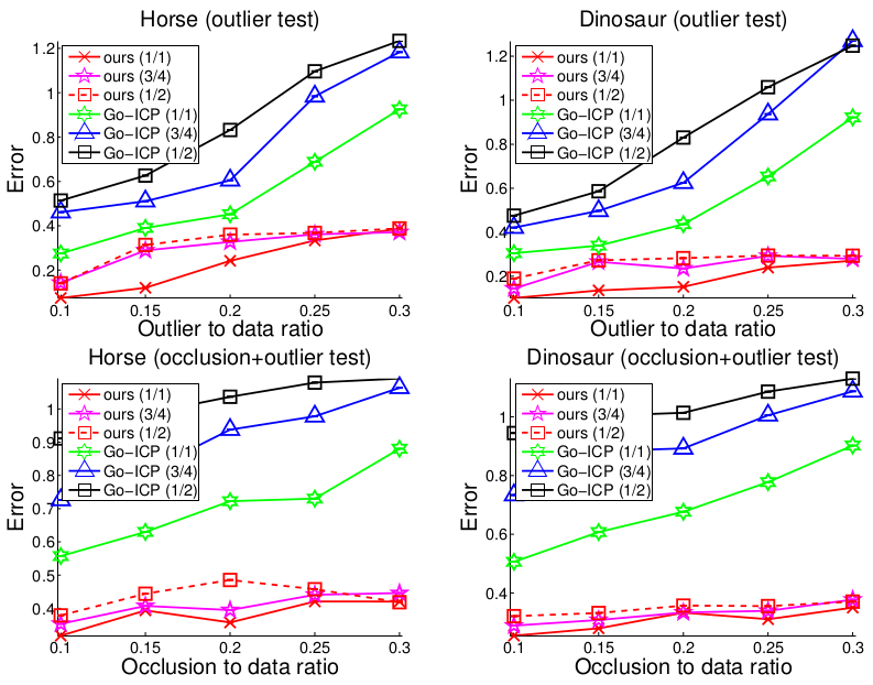
Figure 16: Average matching errors by our method and Go-ICP with different $n_{p}$ values (chosen from $1/2$ to $1/1$ the ground truth value) over 100 random trials for the 3D outlier and occlusion+outlier tests.

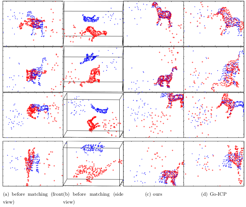
Figure 17: Examples of matching results by our method and Go-ICP in the 3D outlier (top row) and occlusion+outlier (bottom row) tests.

The average running time of our method and Go-ICP are 152.7024 and 1.8105 seconds, respectively.

7 Conclusion

We proposed a new point matching algorithm capable of handling the case that there is only partial overlap between two point sets in this paper. Our algorithm works by reducing the objective function of RPM to a concave function of point correspondence with a low rank structure. The BnB algorithm is then used for optimization. Two cases of transformation, the transformation is linear with respect to its parameters and the 2D/3D similarity transformations, are discussed for our algorithm. We also proposed a new lower bounding scheme which has a k-cardinality linear assignment formulation and can be very efficiently solved. The resulting algorithm is approximately globally optimal, scales well with problem size and is efficient for the 2D case.

Experimental results on both 2D and 3D datasets showed that the proposed method has strong robustness against disturbances and outperforms state-of-the-art methods in terms of robustness to outliers and occlusions with competitive time efficiency.

References

• [1] M. D. Amicoa, A. Lodib, and S. Martello. Efficient algorithms and codes for k-cardinality assignment problems. Discrete Applied Mathematics, 110:25–40, 2001.
• [2] J.-C. Bazin, H. Li, I. S. Kweon, C. P. Vasseur, and K. Ikeuchi. A branch-and-bound approach to correspondence and grouping problems. IEEE Trans. Pattern Analysis and Machine Intelligence, 35(7):1565–1576, 2013.
• [3] J.-C. Bazin, Y. Seo, and M. Pollefeys. Globally optimal consensus set maximization through rotation search. In ACCV, 2012.
• [4] S. Belongie, J. Malik, and J. Puzicha. Shape matching and object recognition using shape contexts. IEEE Trans. Pattern Analysis and Machine Intelligence, 24(4):509–522, 2002.
• [5] P. J. Besl and N. D. McKay. A method for registration of 3-d shapes. IEEE Trans. Pattern Analysis and Machine Intelligence, 14(2):239–256, 1992.
• [6] D. Breitenreicher and C. Schnörr. Model-based multiple rigid object detection and registration in unstructured range data. Int. J. Comput. Vision, 92(1):32–52, Mar. 2011.
• [7] A. P. Bustos, T.-J. Chin, and D. Suter. Fast rotation search with stereographic projections for 3d registration. In CVPR, 2014.
• [8] T. Chen, B. C. Vemuri, A. Rangarajan, and S. J. Eisenschenk. Group-wise point-set registration using a novel cdf-based havrda-charv t divergence. 86(1):111–124, 2010.
• [9] H. Chui and A. Rangarajan. A new point matching algorithm for non-rigid registration. Computer Vision and Image Understanding, 89(2-3):114–141, 2003.
• [10] Y. Deng, A. Rangarajan, S. Eisenschenk, and B. C. Vemuri. A riemannian framework for matching point clouds represented by the schrödinger distance transform. In CVPR, 2014.
• [11] J. Glaunes, A. Trouve, and L. Younes. Diffeomorphic matching of distributions: A new approach for unlabelled point-sets and sub-manifolds matching. In IEEE Conference on Computer Vision and Pattern Recognition (CVPR), pages 712–718, 2004.
• [12] J. Ho, A. Peter, A. Rangarajan, and M.-H. Yang. An algebraic approach to affine registration of point sets. In IEEE Conf. Computer Vision and Pattern Recognition, 2009.
• [13] R. Horst and H. Tuy. Global Optimization, Deterministic Approaches. Springer-Verlag, 1996.
• [14] B. Jian and B. C. Vemuri. A robust algorithm for point set registration using mixture of gaussians. In IEEE International Conference on Computer Vision, volume 2, pages 1246–1251, 2005.
• [15] B. Jian and B. C. Vemuri. Robust point set registration using gaussian mixture models. IEEE Trans. Pattern Analysis and Machine Intelligence, 33(8):1633–1645, 2011.
• [16] R. Jonker and A. Volgenant. A shortest augmenting path algorithm for dense and sparse linear assignment problems. Computing, 38:325–340, 1987.
• [17] J.-H. Lee and C.-H. Won. Topology preserving relaxation labeling for nonrigid point matching. IEEE Trans. Pattern Analysis and Machine Intelligence, 33(2):427–432, 2011.
• [18] H. Li. Consensus set maximization with guaranteed global optimality for robust geometry estimation. In CVPR, 2009.
• [19] H. Li and R. Hartley. The 3d-3d registration problem revisited. In ICCV, 2007.
• [20] W. Lian and L. Zhang. Robust point matching revisited: a concave optimization approach. In European conference on computer vision, 2012.
• [21] W. Lian and L. Zhang. Point matching in the presence of outliers in both point sets: A concave optimization approach. In CVPR, 2014.
• [22] D. G. Lowe. Distinctive image features from scale-invariant keypoints. International Journal of Computer Vision, 2004.
• [23] J. Ma, J. Zhao, J. Tian, Z. Tu, and A. L. Yuille. Robust estimation of nonrigid transformation for point set registration. In CVPR, 2013.
• [24] J. Maciel and J. Costeira. A global solution to sparse correspondence problems. IEEE Trans. Pattern Analysis and Machine Intelligence, 25(2):187–199, 2003.
• [25] A. Myronenko and X. Song. Point set registration: Coherent point drift. IEEE Transactions on Pattern Analysis and Machine Intelligence, 32(12):2262–2275, 2010.
• [26] C. Olsson, F. Kahl, and M. Oskarsson. Branch-and-bound methods for euclidean registration problems. IEEE Transactions on Pattern Analysis and Machine Intelligence, 31(5):783–794, 2009.
• [27] C. H. Papadimitriou and K. Steiglitz. Combinatorial optimization: algorithms and complexity. Dover Publications, INC. Mineola. New York, 1998.
• [28] F. Pfeuffer, M. Stiglmayr, and K. Klamroth. Discrete and geometric branch and bound algorithms for medical image registration. Annals of Operations Research, 196(1):737–765, 2012.
• [29] H. R and Z. A. Multiple View Geometry in Computer Vision (2nd ed.). Cambridge: Cambridge University Press, 2003.
• [30] M. Sofka, G. Yang, and C. V. Stewart. Simultaneous covariance driven correspondence (cdc) and transformation estimation in the expectation maximization framework. In IEEE Conf. Computer Vision and Pattern Recognition, pages 1–8, 2007.
• [31] Y. Tsin and T. Kanade. A correlation-based approach to robust point set registration. In European Conference on Computer Vision, pages 558–569, 2004.
• [32] A. Volgenant. Solving the k-cardinality assignment problem by transformation. European Journal of Operational Research, 157:322–331, 2004.
• [33] F. Wang, B. C. Vemuri, and A. Rangarajan. Groupwise point pattern registration using a novel cdf-based jensen-shannon divergence. In IEEE Conf. Computer Vision and Pattern Recognition, 2006.
• [34] J. Yang, H. Li, and Y. Jia. Go-icp: Solving 3d registration efficiently and globally optimally. In ICCV, 2013.
• [35] A. L. Yuille and J. J. Kosowsky. Statistical physics algorithms that converge. Neural Comput., 6(3):341–356, 1994.
• [36] Z. Zhang. Iterative point matching for registration of free-form curves and surfaces. International Journal of Computer Vision, 13(2):119–152, 1994.
• [37] Y. Zheng and D. Doermann. Robust point matching for nonrigid shapes by preserving local neighborhood structures. IEEE Trans. Pattern Analysis and Machine Intelligence, 28(4):643–649, 2006.