Probing Lepton Flavor Violation Signal via $\gamma\gamma\to\bar{\ell}_{i}\ell_{j}$ in the Left-Right Twin Higgs Model at the ILC

Abstract

To explain the small neutrino masses, heavy Majorana neutrinos are introduced in the left-right twin Higgs model. The heavy neutrinos, together with the charged scalars and the heavy gauge bosons, may contribute large mixings between the neutrinos and the charged leptons, which may induce some distinct lepton flavor violating processes. We will check the $\bar{\ell}_{i}\ell_{j}$ ($i,~{}j=e,~{}\mu,~{}\tau,~{}i\neq j$) productions in the $\gamma$$\gamma$ collision in the left-right twin Higgs model, and find that the production rates may be large in some specific parameter space, in the optimal cases even possible to be detected with reasonable kinematical cuts. we have also shown that these collisions can constrain effectively the model parameters such as the Higgs vacuum expectation value and the right-handed neutrino mass, etc., and may serve as a sensitive probe of this new physics model.

I Introduction

One of the problems of the Standard Model (SM) is that the neutrino oscillation experiments indicate that neutrinos are massive and mix with each other, which manifestly require new physics beyond the SM oscillneutrinos since in SM the neutrino masses and thus Lepton Flavor Violating (LFV) couplings are missing. The LFV signals, however, are predicted in many new physics models, such as supersymmetry susy , topcolor assisted technicolor models tc2-review , little Higgs lh-review , Higgs triple models htm-review , and the Left-Right Twin Higgs (LRTH) lrth-review models, etc.

In the LRTH model, to provide the mass origin of the leptons and to explain the small neutrino masses, right-handed heavy neutrinos are introduced. These right-handed heavy neutrinos can realize the mixings of the neutrinos with the leptons, which can induce LFV processes at the proposed International Linear Collider (ILC)ilc-project , such as the decay $\mu\to e\gamma$ 0711.1238 . We will in this paper will discuss the $\bar{\ell}_{i}\ell_{j}$ ($i,~{}j=e,~{}\mu,~{}\tau,~{}i\neq j$) productions via the $\gamma\gamma$ collision in the LRTH model.

Due to its rather clean environment, the ILC can be an ideal collider to probe new physics. At the ILC, in addition to $e^{+}e^{-}$ collision, one can also realize the $\gamma\gamma$ collision rr-project with the photon beams generated by the backward compton scattering of incident electron- and laser-beams.

The $\gamma\gamma$ collision, however, has two advantages over the $e^{+}e^{-}$ collision of the ILC in probing the LFV interaction rr-advantage ; 0311166 . One is that the process $e^{+}e^{-}\to\bar{\ell}_{i}\ell_{j}$ occurs only via s-channel, and the rates are suppressed by the photon propagator and the neutral gauge boson propagator. On the contrary, the process $\gamma\gamma\to\bar{\ell}_{i}\ell_{j}$ is free of this. Another is that the backgrounds of the $e^{+}e^{-}$ collision may be not so easy to suppressrr-advantage . Since the $\gamma\gamma$ collision may be free of many SM irreducible backgrounds, the LFV productions in $\gamma\gamma$ collision are suitable for detecting the new physics models.

We in this work will study the LFV processes $\gamma\gamma\to\bar{\ell}_{i}\ell_{j}$ ($i\neq j$ and $\ell_{i}=e,~{}\mu,~{}\tau$) induced by the gauge bosons $W^{\pm}$, $W_{H}^{\pm}$ and charged scrlars $\phi^{\pm}$ in LRTH models, at the same time, the heavy neutrinos entering the loop. we will find that, due to the existence of the heavy neutrinos, the production in the LRTH model have different properties and rich phenomenology.

This paper is organized as follows. In Sec. II we briefly review the lepton sector of LRTH model and give the couplings involved in our calculation. In Sec. III, we will discuss the contributions from the gauge bosons and the charged scalars. In Sec.IV, on the base of the former discussion, we will show the parameter constraints related to the processes. Finally, conclusions are given in Sec. V.

II the lepton sector of the LRTH model and the relevant couplings

In the LRTH model lrth-review ; 0711.1238 ; 0611015-su , with the global symmetry $U(4)\times U(4)$, the Higgs field and the twin Higgs in the fundamental representation of each $U(4)$ can be written as $H$ = $(H_{L},H_{R})$ and $\hat{H}$ = $(\hat{H}_{L},\hat{H}_{R})$, respectively. After each Higgs develops a vacuum expectation value (VEV),

$$<H>=(0,0,0,f),\quad<\hat{H}>=(0,0,0,\hat{f}),$$ (1)

the global symmetry $U(4)\times U(4)$ breaks to $U(3)\times U(3)$, with the gauge group $SU(2)_{L}\times SU(2)_{R}\times U(1)_{B-L}$ down to the SM $U(1)_{Y}$. After the breaking, there are six massive gauge bosons left: the SM $Z$ and $W^{\pm}$, and extra heavier bosons, $Z_{H}$ and $W_{H}^{\pm}$. And eight scalars are left: one neutral pseudoscalar, $\phi^{0}$, a pair of charged scalars $\phi^{\pm}$, the SM physical Higgs $h$, and an ${\rm SU}(2)_{L}$ twin Higgs doublet $\hat{h}=(\hat{h}_{1}^{+},\hat{h}_{2}^{0})$.

Neutrino oscillations oscillneutrinos imply that neutrinos are massive, and the LRTH models try to explain the origin of the neutrino masses and mass hierarchy. Three families doublets ${\rm SU}(2)_{L,R}$ are introduced in the LRTH models to provide lepton masses,

$$L_{L\alpha}=-i\left(\begin{array}[]{c}~{}\nu_{L\alpha}\\ l_{L\alpha}\end{array}\right),~{}~{}~{}L_{R\alpha}=\left(\begin{array}[]{c}~{}\nu_{R\alpha}\\ l_{R\alpha}\end{array}\right),$$ (6)

where the family index $\alpha$ runs from 1 to 3.

In the same way as the first two generations of quarks, the charged leptons also obtain their masses via non-renormalisable dimension $5$ operators, which for the lepton sector can be written as

$${y_{l}^{ij}\over\Lambda}(\bar{L}_{Li}H_{L})(H_{R}^{\dagger}{L}_{Rj})+{y_{\nu}^{ij}\over\Lambda}(\bar{L}_{L,i}\tau_{2}H_{L}^{*})(H_{R}^{T}\tau_{2}{L}_{Rj})+{\rm{H.c.}},$$ (7)

which will give rise to lepton Dirac mass terms $y_{\nu,l}^{ij}f^{2}/\Lambda$, once $H_{L}$ and $H_{R}$ acquire VEVs.

The Majorana nature of the left- and right-handed neutrinos, however, makes one to induce Majorana terms ( only the mass section) in dimension 5 operators,

$${c_{L}\over\Lambda}\,\left(\overline{L}_{L\alpha}\tau_{2}H_{L}^{\dagger}\right)^{2}+{\rm H.c},\qquad{c_{R}\over\Lambda}\,\left(\overline{L}_{R\alpha}\tau_{2}H_{R}^{\dagger}\right)^{2}+{\rm H.c.}~{}.\$$ (8)

Once $H_{L}~{}(H_{R})$ obtains a VEV, both neutrino chiralities obtain Majorana masses via these operators, the smallness of the light neutrino masses, however, can not be well explained.

Then, if we assume that the twin Higgs $\hat{H}_{R}$ (which is forbidden to couple to the quarks to prevent the heavy top quark from acquiring a large mass of order $y\hat{f}$) couples to the right-handed neutrinos, one finds that 0711.1238

$${c_{\hat{H}}\over\Lambda}\,\left(\overline{L}_{R\alpha}\tau_{2}\hat{H}_{R}^{\dagger}\right)^{2}+{\rm H.c.}~{},$$ (9)

which will give a contribution to the Majorana mass of the heavy right-handed neutrino, in addition to those of Eq.(8).

After the electroweak symmetry breaking, $H_{R}$ and $\hat{H}_{R}$ get VEVs, $f$ and $\hat{f}$ (Eq.(1)), respectively, we can derive the following seesaw mass matrix for the LRTH model in the basis ($\nu_{L}$,$\nu_{R}$):

$${\cal M}=\left(\begin{array}[]{cc}c{v^{2}\over 2\Lambda}&y_{\nu}{vf\over\sqrt{2}\Lambda}\\ y_{\nu}^{T}{vf\over\sqrt{2}\Lambda}&c{f^{2}\over\Lambda}+c_{\hat{H}}{\hat{f}^{2}\over\Lambda}\end{array}\right)~{}.$$ (10)

In the one-generation case there is two massive states, a heavy ($\sim\nu_{R}$) and a light one. For the case that $v<f<\hat{f}$, the masses of the two eigenstates are about $m_{\nu_{heavy}}\sim c_{\hat{H}}{\hat{f}^{2}\over\Lambda}$ and $m_{\nu_{light}}={cv^{2}\over 2\Lambda}$ 0711.1238 .

The Lagrangian in Eq.(7) induces neutrino masses and the mixings of different generation leptons, which may be a source of lepton flavour violating 0711.1238 .

We consider the contributions of the heavy gauge boson, $W_{H}$, and the charged scalars, $\phi^{\pm}$, too. The relevant vertex interactions for these processes are explicated in the followings:

$$\phi^{-}\bar{l}\nu_{L,R}:\frac{i}{f}(m_{l_{L},\nu_{R}}P_{L}-m_{\nu_{L},l_{R}}P_{R})V_{H}\sim ic_{H}\frac{{\hat{f}}^{2}}{\Lambda f}P_{L},$$ (11)

$$W^{-}_{L,R}\bar{l}\nu_{L,R}:\frac{e}{\sqrt{2}s_{w}}\gamma_{\mu}P_{L,R}V_{H}.$$ (12)

where $V_{H}$ is the mixing matrix of the heavy neutrino and the leptons mediated by the charged scalars and the heavy gauge bosons. The vertexes of $\phi^{-}\bar{l}\nu_{L,R}$ can also be expressed in the coupling constants. The $\phi^{-}\bar{l}\nu_{R}$, for example, is also written as $ic_{H}\frac{\hat{f}^{2}}{\Lambda f}P_{L}$ if we neglect the charged lepton masses and take $m_{\nu_{h}}=c_{H}\hat{f}^{2}/\Lambda$.

III Calculations

III.1 The Distribution Functions in the $\gamma\gamma$ collision

For the $\gamma\gamma$ collision at the ILC, the photon beams are generated by the backward Compton scattering of incident electron- and laser-beams just before the interaction point. The events number is obtained by convoluting the cross section with the photon beam luminosity distribution and for the $\gamma\gamma$ collider the events number is obtained by

$$N_{\gamma\gamma\to\bar{\ell}_{i}\ell_{j}} = \int{\rm d}\sqrt{s_{\gamma\gamma}}\frac{{\rm d}{\cal L}_{\gamma\gamma}}{{\rm d}\sqrt{s_{\gamma\gamma}}}\hat{\sigma}_{\gamma\gamma\to\bar{\ell}_{i}\ell_{j}}(s_{\gamma\gamma})\equiv{\cal L}_{e^{+}e^{-}}~{}\sigma_{\gamma\gamma\to\bar{\ell}_{i}\ell_{j}}(s_{e^{+}e^{-}}),$$ (13)

where ${\rm d}{\cal L}_{\gamma\gamma}/{\rm d}\sqrt{s_{\gamma\gamma}}$ is the photon beam luminosity distribution and $\sigma_{\gamma\gamma\to\bar{\ell}_{i}\ell_{j}}(s_{e^{+}e^{-}})$, with $s_{e^{+}e^{-}}$ being the energy-square of $e^{+}e^{-}$ collision, is defined as the effective cross section of $\gamma\gamma\to\bar{\ell}_{i}\ell_{j}$. In optimum case, $\sigma_{\gamma\gamma\to\bar{\ell}_{i}\ell_{j}}$ can be written as distribution

$$\sigma_{\gamma\gamma\to\bar{\ell}_{i}\ell_{j}}(s_{e^{+}e^{-}}) = \int_{\sqrt{a}}^{x_{max}}2z{\rm d}z~{}\hat{\sigma}_{\gamma\gamma\to\bar{\ell}_{i}\ell_{j}}(s_{\gamma\gamma}=z^{2}s_{e^{+}e^{-}})\int_{z^{2}/x_{max}}^{x_{max}}\frac{{\rm d}x}{x}~{}F_{\gamma/e}(x)~{}F_{\gamma/e}(\frac{z^{2}}{x}),$$ (14)

where $F_{\gamma/e}$ denotes the energy spectrum of the back-scattered photon for unpolarized initial electron and laser photon beams given by

$$F_{\gamma/e}(x) = \frac{1}{D(\xi)}\left(1-x+\frac{1}{1-x}-\frac{4x}{\xi(1-x)}+\frac{4x^{2}}{\xi^{2}(1-x)^{2}}\right).$$ (15)

The definitions of parameters $\xi$, $D(\xi)$ and $x_{max}$ can be found in distribution . In our numerical calculation, we choose $\xi=4.8$, $D(\xi)=1.83$ and $x_{max}=0.83$.

III.2 Amplitudes for $\gamma\gamma\to\bar{\ell}_{i}\ell_{j}$

Via the coupling in Eq.(11), the Feynman diagrams for the production $\gamma\gamma\to\bar{\ell}_{i}\ell_{j}$ mediated by the charged gauge bosons are shown in Fig. 1. The contributions from the charged scalars have the similar structure as that from the gauge boson. That is, if the boson lines change into scalar lines in Fig. 1 and Fig. 2, they will become to the Feynman diagrams contributed by the charged scalars, which have not shown explicitly.

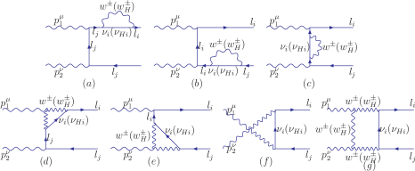
Figure 1: Feynman diagrams for the production $\gamma\gamma\to\bar{\ell}_{i}\ell_{j}$ in the LRTH model mediated by the heavy and light gauge bosons $W_{L,R}^{\pm}$. Those with the two photon lines crossed are not shown.

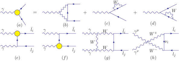
Figure 2: Feynman diagrams for the production $\gamma\gamma\to\bar{\ell}_{i}\ell_{j}$ in the LRTH model, with the triangle- and the self-energy-diagrams replaced by the tree level vertex (a), i.e., (b)(c)(d).

It can also be seen that we have changed Figs.1(a), 1(b), 1(c), 1(d) and 1(e) into Figs.2(e) and 2(f) via extracting a vertex shown as Figs.2(a), 2(b), 2(c) and 2(d)0702264 . To obtain this, we split the propagator in Fig.1(c) into two parts:

$$M_{c}\propto\frac{i}{\not{\hbox{\kern-2.1pt$q$}}-m_{i}}i\Sigma(q)\frac{i}{\not{\hbox{\kern-2.1pt$q$}}-m_{j}}=\frac{i(\not{\hbox{\kern-2.1pt$q$}}+m_{i})}{m_{j}^{2}-m_{i}^{2}}\ i\Sigma(q)\ \frac{i}{\not{\hbox{\kern-2.1pt$q$}}-m_{j}}+\frac{i}{\not{\hbox{\kern-2.1pt$q$}}-m_{i}}\ i\Sigma(q)\ \frac{i(\not{\hbox{\kern-2.1pt$q$}}+m_{j})}{m_{i}^{2}-m_{j}^{2}}.$$ (16)

In the right-handed terms of Eq. (16), the first term together with Fig.1 (a, d), and the second term together with Fig.1(b, e) can be collected into a vertex, irrespectively. Then the momentum dependent $\bar{\ell}_{i}\ell_{j}\gamma$ vertex, after this arrangement, can be defined as,

$$\Gamma^{{}^{\prime}\bar{\ell}_{i}\ell_{j}\gamma}_{\mu}(p_{i},p_{j}) = \Gamma_{\mu}^{\bar{\ell}_{i}\ell_{j}\gamma}(p_{i},p_{j})+i\Sigma(p_{i})\frac{i(\not{\hbox{\kern-2.1pt$p$}}_{i}+m_{j})}{m_{i}^{2}-m_{j}^{2}}\Gamma_{\mu}^{\bar{l}l^{\prime}\gamma}+\Gamma_{\mu}^{\bar{l}l^{\prime}\gamma}\frac{i(\not{\hbox{\kern-2.1pt$p$}}_{j}+m_{i})}{m_{j}^{2}-m_{i}^{2}}\ i\Sigma(p_{j}),$$ (17)

where $\Gamma_{\mu}^{\bar{\ell}_{i}\ell_{j}\gamma}$ is the penguin diagram contribution to the total $\bar{\ell}_{i}\ell_{j}\gamma$ vertex, then the calculation of Fig.1 (a-e) is equivalent to the calculation of the ”tree” level process depicted in Fig.2 (a) and (b), which obviously has a simpler structure.

As for the calculation of the $\bar{\ell}_{i}\ell_{j}\gamma$ vertex, we can firstly give the results from the Lorentz structure, To discuss the contribution of the self energy diagrams, we take Fig.2(c) as an example, and the amplitude can be written as,

$${\cal M}_{c}\sim\gamma^{\rho}\frac{1}{\not{\hbox{\kern-2.1pt$p$}}-\not{\hbox{\kern-2.1pt$k$}}-m_{\nu_{H}}}\gamma_{\rho}\frac{1}{\not{\hbox{\kern-2.1pt$p$}}}\gamma^{\mu}\cdot\bar{\ell}_{i}\ell_{j}\epsilon_{\mu}.$$ (18)

The electromagnetic gauge invariance $\partial_{\mu}{\cal M}=0$ has required this term vanishing. So does Fig.2(d).

So there is only the Fig.2(b) left. When we sum over all the diagrams corresponding to the three intermediate mass eigenstate, note that,

$$\sum\limits_{i}\{\frac{U^{*}_{ei}U_{\mu i}}{(p+k)^{2}-m^{2}_{\nu_{H}}}\} = \sum\limits_{i}U^{*}_{ei}U_{\mu i}\{\frac{1}{(p+k)^{2}}+\frac{m_{i}^{2}}{[(p+k)^{2}]^{2}}+...\}$$ (19)

$$= \sum\limits_{i}\frac{U^{*}_{ei}U_{\mu i}m^{2}_{\nu_{H}}}{[(p+k)^{2}]^{2}}+...,$$

the leading term vanishes via the GIM mechanism, $\sum\limits_{i}U^{*}_{ei}U_{\mu i}=0.$ The Second term, with more powers of $k$ in the denominator, has already cleared away the UV divergence.

The penguin contributions from the heavy gauge bosons and the charged scalars in unitary gauge ($\xi\to\infty$), which are calculated by hands, via Feynman parameterization and Wick rotation, can be written asl-f-li

$${\cal M}_{W_{H}} = \frac{ce^{3}}{(\sqrt{2}s_{W})^{2}}\frac{m_{i}}{64\pi m_{W_{H}}^{4}}\bar{u}_{i}(p)(1-\gamma_{5})(2p\cdot\epsilon-m_{i}\gamma\cdot\epsilon)u_{j}(p-k)$$ (20)

$${\cal M}_{H_{\pm}} = -2e\frac{cm_{i}}{32\pi f^{2}m_{H}^{2}}\bar{u}_{i}(p)(1-\gamma_{5})(2p\cdot\epsilon-m_{i}\gamma\cdot\epsilon)u_{j}(p-k)$$ (21)

where $c=\sum\limits_{i}U^{*}_{ei}U_{\mu i}m^{2}_{i\nu_{H}}$ and $m_{i\nu_{H}}$ is the ith generation heavy neutrino mass. $p,~{}k$ is the momentum of production heavier lepton and the photon of the vertex, respectively, and $m_{i}$ is the heavier lepton mass.

As for the box diagram Fig.2(g) and the bosonic quadruple interaction in Fig.2(h), we have use the calculating tool of LoopToolslooptools .

IV Numerical results

In our calculations, we neglect terms proportional to $v^{2}/f^{2}$ in the new gauge boson masses and also in the relevant Feynman rules. We take the SM parameters as pdg-2016 :

$$m_{e}=0.0051\ {\rm GeV},\quad\quad m_{\mu}=0.106\ {\rm GeV},\quad\quad m_{\tau}=1.777\ {\rm GeV},$$

$$m_{Z}=91.2\ {\rm GeV},\quad\quad\quad s^{2}_{W}=0.231,\quad\quad\alpha_{e}=1/128.8.$$

The internal charged lepton masses, $m_{e},~{}m_{\mu},~{}m_{\tau}$, however, will be neglected since they are much lighter than the gauge bosons, the charged scalars, or the right-handed neutrinos.

When the gauge boson is mediated in the loop, just as shown in Fig. 1 and Fig. 2, the relevant parameters are the masses of the gauge bosons $m_{W},~{}m_{W_{H}}$ and the heavy neutrino $m_{\nu_{H}}$. On the other side, the heavy charged bosons may also contribute large to the lepton flavor changing processes, which can be realized by replacing the heavy gauge bosons with the charged scalars $\phi^{\pm}$ in Fig.1 and Fig. 2.

In the Higgs mediated process, in addition to the masses of the charged scalars $m_{\phi}$ and the heavy neutrino $m_{\nu_{H}}$, the breaking scales $f$, $\hat{f}$ are also dependent parameters. The light neutrino masses and the charged leptons mixings to the light neutrinos $c_{i}$ ($\phi^{-}\bar{l}\nu_{L,R}$) are quite small, so we here neglect the contributions mediated by the light neutrinos. We will focus on the heavy neutrinos, which coupling to charged leptons via the charged scalars is proportional to the heavy neutrino mass, i.e, $\sim c_{H}\frac{\hat{f}^{2}}{\Lambda f}$.

For the masses of the charged scalars and the heavy gauge bosons, we vary their ranges as: $200\leq m_{\phi}\leq 1000$ GeV charged_higgs_mass (sometimes, extending to $100$ GeV) and $1000\leq M_{W_{H}}\leq 5000$ GeV w_h_constraints .

Note that in the couplings of $\phi^{+}(W_{H}^{+})\nu_{H}^{k}\bar{\ell}$ there exist the mixing terms $V_{H}^{kl}$s, which parameterize the interactions of the charged leptons with the heavy neutrinos, mediated by both $\phi^{\pm}$ and $W_{H}^{+}$, and they can be chosen as the Maki-Nakagawa-Sakata (MNS) matrix $V_{\text{MNS}}$, which diagonalizes the neutrino mass matrix massMaki:1962mu ; 07124019 :

$$V_{\text{MNS}}=\left(\begin{array}[]{ccc}c_{12}c_{13}&s_{12}c_{13}&s_{13}e^{-i\delta}\\ -s_{12}c_{23}-c_{12}s_{23}s_{13}e^{i\delta}&c_{12}c_{23}-s_{12}s_{23}s_{13}e^{i\delta}&s_{23}c_{13}\\ s_{12}s_{23}-c_{12}c_{23}s_{13}e^{i\delta}&-c_{12}s_{23}-s_{12}c_{23}s_{13}e^{i\delta}&c_{23}c_{13}\end{array}\right)\,,$$ (22)

where $s_{ij}\equiv\sin\theta_{ij}$ and $c_{ij}\equiv\cos\theta_{ij}$. $\delta$ is the CP-phase.

Three mixing angles $\theta_{12}$, $\theta_{13}$, $\theta_{23}$ can be chosen as free parameters since the they are different from those of the SM. The contribution of the CP-phase $\delta$, varying from $0\sim 2\pi$, can be a free parameter. But we take firstly the three mixing angles $\theta_{12}$, $\theta_{13}$, $\theta_{23}$ and the CP-phase $\delta$ assolar ; atm ; acc ; daya-bay ; delta

$$\sin^{2}2\theta_{12}\simeq 0.86\,,~{}~{}~{}~{}\sin^{2}2\theta_{23}\simeq 1\,,~{}~{}~{}~{}\sin^{2}2\theta_{13}\simeq 0.089\,,~{}~{}~{}~{}\delta\simeq\pi,$$ (23)

and in the final discussion we vary them as free parameters.

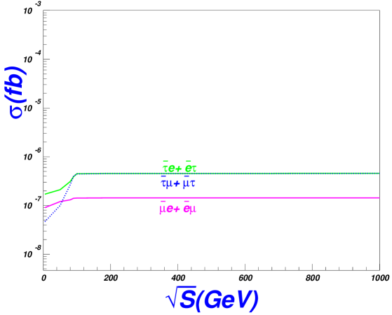
Figure 3: The cross sections of the process $\gamma\gamma$ $\to\bar{\mu}e+\bar{e}\mu$, $\to\bar{\mu}e+\bar{e}\mu$ and $\to\bar{\mu}e+\bar{e}\mu$ vary as the increasing centre-of-mass energy.

IV.1 The SM Background of the Flavor Changing Processes

The SM backgrounds of the flavor changing production is quite small, since these processes are prohibited in the tree level and suppressed largely in the one-loop levelsusy-r-con1 . The main backgrounds of the $\tau\bar{e}$ may be $\gamma\gamma\to\tau^{+}\tau^{-}\to\tau\nu_{e}\bar{\nu}_{\tau}\bar{e}$, $\gamma\gamma\to W^{+}W^{-}\to\tau\nu_{\tau}\nu_{e}\bar{e}$ and $\gamma\gamma\to\tau\bar{e}\nu_{\tau}\nu_{e}$, which are suppressed to be $~{}9.7\times 10^{-4}$ fb, $~{}1.0\times 10^{-1}$ fb and $~{}2.4\times 10^{-2}$ fb.If $3.45\times 10^{2}$ fb^-1 integrated luminosity of the photon collision tesla is chosen, the production rates of $\gamma\gamma\to\mu\bar{e},~{}\tau\bar{e},~{}\tau\bar{\mu}$ should be larger than $10^{-2}$ fb to get the $3\sigma$ observing significance susy-r-con1 ; rvio-susy-rrll .

In the calculation, to avoid the collinear divergence, we require that the scattering angle cut $|\cos\theta_{e}|<0.9$ and the transverse momentum cut $p^{e}_{T}>20{\rm~{}GeV}$, which are the same as the cuts in Ref. susy-r-con1 . Therefore the requirement of the cross section $10^{-2}$ fb can be used to constraint the parameter such as $f$, $m_{\phi}$, $m_{W_{H}}$ and $m_{\nu_{H}}$, etc and give the contours between them, just shown as Fig. (4), Fig. (6).

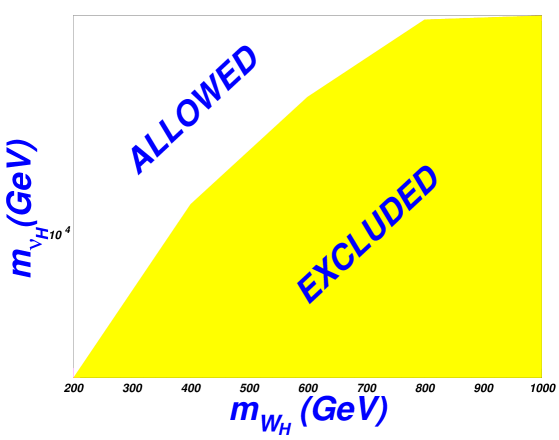
Figure 4: The contour of the process $\gamma\gamma\to\bar{\mu}e+\bar{e}\mu$, between $m_{W_{H}}$ and $m_{\nu_{H}}$.

IV.2 The Contour of $m_{W_{H}}$ and $m_{\nu_{H}}$ in the $W_{H}$-mediated process

Since the relation of parameters in $\gamma\gamma\to\bar{\ell}_{i}\ell_{j}$ mediated by the heavy $W_{H}$ is a little simple, we will begin from this channel to discuss the dependence of the parameters. Of course, the process $\gamma\gamma\to\bar{\ell}_{i}\ell_{j}$ should receive the contribution from both the heavy gauge bosons and the charged scalars, and we will discuss this later.

To find the influence of the center-of-mass energy, we plot in Fig.3 that the cross section changing with the increasing $\sqrt{S}$, and the results are in our expectation. We can see that the production rates of the three channels are almost in the same order, and the trend of every channel is almost flat, so in our following discussion, we will take $\sqrt{S}=200$ GeV and neglect the minor difference induced by it.

From Fig.3, we also see that the three curves in our precision range are almost the same, at least in the same order, so we in the followings will only consider one process, for example, the $\bar{\mu}e+\bar{e}\mu$ production.

We will give the contour of $m_{W_{H}}$ and $m_{\nu_{H}}$ firstly in Fig. 4, in which, the $W_{H}$ is taken between $200$ and $1000$ GeV, but in actual case, we should have a larger $m_{W_{h}}$, e.g., larger than $1000$ GeV, so we can conclude that if $10^{-2}$ fb limit is assumed, the possibility for $m_{W_{H}}$ and $m_{\nu_{H}}$ to survive together is quite small.

IV.3 The Contributions from the $f$, $m_{\phi}$, $m_{\nu_{H}}$ and $m_{W_{H}}$

The VEVs $f$ and $\hat{f}$ of the two Higgses $H$ and $\hat{H}$, respectively, are taken as $500\leq f\leq 5000$ and $\hat{f}=10f$ in this work 0711.1238 . The parameters mainly involved are the parameters $m_{W_{H}}$, $m_{\phi}$, $m_{\nu_{H}}$, the Higgs VEV $f$, and the mixing matrix $V_{H}$, which will be emphatically discussed.

We show in Fig.5 the dependence of parameters $f$, the scalar mass $m_{\phi}$, the heavy neutrino mass $m_{\nu_{H}}$ and the heavy chaged boson mass $m_{W_{H}}$. We also see from in Fig.5 that the dependence of $f$, $m_{\nu_{H}}$, $m_{\phi}$ and $m_{W_{H}}$ is large enough to be detectable in some parameter space, for the $10^{-2}$ limit, with the requirements: $f<1400GeV,~{}m_{\nu_{H}}>6000GeV$ and looser $m_{\phi},~{}m_{W_{H}}$.

We notice that in Fig.5 (a)(b), the $f$ and the $m_{\nu_{H}}$ dependence, which have opposite influence on the production rates, i.e., the cross section is increasing with a increasing $m_{\nu_{H}}$, but a decreasing $f$, which can be understandable since from Eq.(11), we can see that the coupling of $\phi\bar{l}\nu_{H}$ proportional to $m_{\nu_{H}}$, while inverse proportional to $f$.

(a)

(b)

(c)

(d)

Figure 5: The cross section $\sigma$ of the processes $\gamma\gamma\to\bar{\tau}\mu$ as a function of the breaking $f$, the scalar mass $m_{\phi}$, the heavy neutrino mass $m_{\nu_{H}}$ and the heavy charged boson mass $m_{W_{H}}$, respectively.

(a)

(b)

(c)

Figure 6: The contour of $f$ and $m_{\nu_{H}}$(a), of $m_{\phi}$ and $f$(b), and of $m_{\phi}$ and $m_{\nu_{H}}$ (c)

(a)

(b)

(c)

(d)

Figure 7: The production rates as functions of $c_{12}$, $c_{13}$, $c_{23}$, and $\delta$.

The production rates with the $m_{\phi}$ in Fig.5(c), are large, and the total range of the vertical axis is not too wide: 0.009 -0.018 fb, which provide the possibility to measure the scalar mass.

From Fig.5 (d), we can see that the $m_{W_{H}}$ dependence seems quite large, the cross sections, however, the contributions of $m_{W_{H}}$ and $f$ are not related with each other, since the couplings of $W_{H}\bar{l}\nu_{H}$ in Eq.(12) do not comprise the breaking parameter $f$, so in Fig. 5(d) the curve of the cross section on $m_{W_{H}}$ is flat especially when $m_{W_{H}}$ becomes large, which is because in the total production, the scalar contribution dominates so that the change of the heavy gauge boson mass can not affect the production order.

Since in Fig.5 the dependence of $f$, the scalar mass $m_{H}$ and the heavy neutrino mass $m_{\nu_{H}}$ is large, Fig.6 will show the contour of $m_{\nu_{H}}$ vs. $f$ (a), $f$ vs. $m_{H}$(b) and $m_{\nu_{H}}$ vs. $m_{H}$(c).

In Fig. 6(a)(c) we can see that the two contours have similar trend with the changing $m_{\nu_{H}}$. With increasing $m_{\nu_{H}}$, the cross section will increase too, so a large $m_{\nu_{H}}$ is favored. We also see in Fig. 6 that in our grossly discussion, if $f>1000$ GeV, for the rates to arrive at the detectable production rates, $m_{\nu_{H}}$ must be larger than $8190$ GeV, while the scalar mass should be smaller than $300$ GeV.

In Fig. 6(b) we see the contour between $m_{\phi}$ and $f$, and the surviving space is quite small, which is understandable since the largest contribution comes from the mass of the heavy neutrino, and we take $m_{\nu_{H}}=1000$ GeV in Fig.6 (b), which is not enough to obtain a big production rate, so to arrive at the required cross sections, $f$ or $m_{\phi}$ should not too large, which limit them in a small possible space.

From Fig. 6(a)(b)(c), we see that the right-handed neutrino mass contributes largest to the cross section, so this process may serve as a severe constrain to the mass of the heavy neutrino.

Although we have discussed the dependences on $m_{W_{H}}$, $f,~{}m_{\phi},~{}m_{\nu_{H}}$, (see Figs. 4, 3, 5, and 6), we have not considered changing generation mixings, since we have fixed them as the lepton mixing parameters [as in Eq. (23)]. In fig.7 we free them and plot the dependence of these mixing parameters. We find that the cross sections vary large in some ranges but in total are gradual, especially the curve of Fig.7(d).

In Fig.7(a)(b), there are sharp points when $c_{12}=0$ or $c_{13}=0$, and we can find the reason in the expression of the mixing matrix in Eq.(22), in which, the element $V_{12}$ and $V_{13}$ are proportional to $s_{12}$ and $s_{13}$, respectively. $c_{12}=0$ or $c_{13}=0$, $s_{12}=1$ or $s_{13}=1$ will contribute quite large.

V Conclusion

Charged scalar- and gauge boson- mediated lepton flavor changing productions of $\bar{\ell}_{i}\ell_{j}$ ($i\neq j$) via $\gamma\gamma$ collision at the ILC have been performed. We find that in a certain parameter space, the production rates of $\gamma\gamma\to\bar{\ell}_{i}\ell_{j}$ ($i\neq j$) may arrive at $10^{-2}$ fb, which means that we may have serval events each year for the designed luminosity of about $345$ fb^-1/year at the ILC. Due to the negligible observation of such $\bar{\ell}_{i}\ell_{j}$ events in the SM, it would be a detection to the left-right twin Higgs models in the lepton sector.

And more important, if we cannot detect the process, this may constrain the parameters strictly. For example, if the process is undetectable, we can give a upper limit of the Higgs breaking scale $f$. We can see from Fig.5(a), to arrive at the cross section $10^{-2}$ fb, $f$ should be less than $1.4$ TeV in the set parameter space.

Moreover, since the LFV couplings are closely related to the heavy neutrino masses, we may obtain interesting information for the heavy neutrino masses if we could see any signature of the LFV processes. In Fig.5(b), to arrive at the cross section $10^{-2}$ fb, the heavy neutrino mass $m_{\nu_{H}}$ should be larger than $6$ TeV in the given parameter space.

Therefore, these LFV processes may serve as a sensitive probe and a strict constraint of this kind new physics models.

VI Acknowledgments

This work was supported by Excellent Youth Foundation of Zhengzhou University under grands No. 1421317053 and 1421317054, and the Natural Science Foundation of China under grant No. 11605110.

References

- (1) See, for example, M. C. Gonzalez-Garcia and Y. Nir, Rev. Mod. Phys. 75, 345(2003); V. Barger, D. Marfatia, and K. Whisnant, Int. J. Mod. Phys E12, 569(2003); A. Y. Smimov, arXiv: hep-ph/0402264; M. C. Gonzalez-Garcia and M. Maltoni, Physics Reports 460, 1(2007)
- (2) Y. A. Golfand and E. P. Likhtman, JETP Lett. 13, 323(1971) [Pis’ma Zh. Eksp. Teor. Fiz. 13,452 (1971)]; D. V. Volkov and V. P. Akulov, Phys. Lett. B 46, 109 (1973); J. Wess and B. Zumino, Nucl. Phys. B70, 39 (1974).
- (3) C. T. Hill, Phys. Lett. B345, 483 (1995); K. Lane and E. Eichten, Phys. Lett. B352, 382 (1995); K. Lane, Phys. Lett. B433, 96 (1998); G. Cvetic,Rev. Mod. Phys.71, 513 (1999); C. T. Hill and E. H. Simmons, Phys. Rep. 381, 235 (2003).
- (4) N. Arkani-Hamed, A. G. Cohen, T. Gregoire, E. Katz, A. E. Nelson, and J. G. Wacker, J. High Energy Phys. 08 (2002) 021; J. G. Wacker, Nucl. Phys. B, Proc. Suppl. 117, 728 (2003); M. Schmaltz, Nucl. Phys. B, Proc. Suppl. 117, 40 (2003); M. Schmaltz, D. Tucker-Smith, Annu. Rev. Nucl. Part. Sci. 55, 229 (2005).
- (5) J. Schechter and J. W. F. Valle, Phys. Rev. D 22, 2227 (1980); T. P. Cheng and L. F. Li, Phys. Rev. D 22, 2860 (1980).
- (6) Z. Chacko, H.-S. Goh, R. Harnik, Phys. Rev. Lett.96, 231802(2006); Z. Chacko, Y. Nomura, M. Papucci, and G. Perez, J. High Energy Phys. 0601:126,2006, Z. Chacko, H. Goh, R. Harnik, J. High Energy Phys. 0601 (2006) 108.
- (7) See the web: http://www.linearcollider.org/ILC/Publications/Reference-Design-Report. H. Braun et al., CLIC-NOTE-764, [CLIC Study Team Collaboration], CLIC 2008 parameters, http://www.clic-study.org.
- (8) Asmaa Abada and Irene Hidalgo, Phys. Rev. D77, (2008) 113013.
- (9) B. Badelek, et al, Int.J.Mod.Phys.A19 (2004), 5097-5186; J. Gronberg, arXiv:1203.0031; R. Nisius, arXiv:hep-ex/9811024; A. Rosca, Euro. Phys. J. C33, s1044 (2004).
- (10) K. J. Abraham, K. Whisnant and B.-L. Young, Phys. Lett. B 419, 381 (1998).
- (11) Jun-jie Cao, Guo-li Liu, Jin Min Yang, Euro. Phys. J. C41, (2005) 381.
- (12) Hock-Seng Goh, Shufang Su Phys. Rev. D75, 075010 (2007).
- (13) I. F. Ginzburg et al., Nucl. Instrum 219, 5 (1984); V. I. Telnov, Nucl. Instrum. Meth. 294, 72 (1990).
- (14) J.J.Cao, G.Eilam, M.Frank, K.Hikasa, G.L.Liu, I.Turan, J. M. Yang Phys. Rev. D75,(2007)075021.
- (15) Gauge theory of elementary particle physics, T Cheng L Li D Gross - Oxford University Press - 1984.
- (16) T. Hahn and M. Perez-Victoria, Comput. Phys. Commun. 118, 153 (1999), T. Hahn, PoS ACAT2010, (2010) 078.
- (17) C. Patrignani et al. (Particle Data Group), Chin. Phys. C, 40, 100001 (2016).
- (18) M. Acciarri et al., [L3 Collaboration], Phys. Lett. B496, 200034; LEP Higgs Working Group, hep-ex/0107031; ALEPH collaboration, Phys. Lett. B487, 2000253. T. Plehn, Phys. Rev. D67, (2003) 014018. E. L. Berger, T. Han, J. Jiang, T. Plehn, Phys. Rev. D71, (2005) 115012. Alejandra Melfo, Miha Nemevsek, Fabrizio Nesti, Goran Senjanovic, Yue Zhang, Phys. Rev. D85, (2012) 055018.
- (19) CMS Collaboration, arXiv:1612.09274.
- (20) Z. Maki, M. Nakagawa and S. Sakata, Prog. Theor. Phys. 28, 870 (1962).
- (21) A.G. Akeroyd, Mayumi Aoki, Hiroaki Sugiyama, Phys. Rev. D77, (2008) 075010.
- (22) B. T. Cleveland et al., Astrophys. J. 496, 505 (1998); W. Hampel et al. [GALLEX Collaboration], Phys. Lett. B 447, 127 (1999); J. N. Abdurashitov et al. [SAGE Collaboration], J. Exp. Theor. Phys. 95, 181 (2002); [Zh. Eksp. Teor. Fiz. 122, 211 (2002)] J. Hosaka et al. [Super-Kamkiokande Collaboration], Phys. Rev. D 73, 112001 (2006); B. Aharmim et al. [SNO Collaboration], Phys. Rev. Lett. 101, 111301 (2008); C. Arpesella et al. [The Borexino Collaboration], Phys. Rev. Lett. 101, 091302 (2008).
- (23) Y. Ashie et al. [Super-Kamiokande Collaboration], Phys. Rev. D 71, 112005 (2005). J.L. Raaf [Super-Kamiokande Collaboration], J. Phys. Conf. Ser. 136, 455 022013 (2008). 456.
- (24) M. H. Ahn et al. [K2K Collaboration], Phys. Rev. D 74, 072003 (2006);P. Adamson et al. [MINOS Collaboration], Phys. Rev. Lett. 101, 131802 (2008).
- (25) F. P. An, et. al., [Daya Bay Collaboration], Chin.Phys. C37 (2013) 011001.
- (26) Shu Luo, Zhi-zhong Xing, Phys. Rev. D86, (2012) 073003; Zhi-Zhong Xing, Chin. Phys. C36, (2012) 281.
- (27) Badelek B et al., Int. J. Mod. Phys. A, 2004, 19: 5097-5186.
- (28) M. Cannoni, C. Carimalo, W. Da Silva, O. Panella, Phys. Rev. D72, (2005) 115004; Erratum-ibid. D72, (2005) 119907.
- (29) Cao J, Wu L, Yang J. Nucl. Phys. B, 2010, 829: 370-382; Sun Yan-Bin, Han Liang, Ma Wen-Gan, Tabbakh Farshid, Zhang Ren-You, Zhou Ya-Jin, J. High Ener. Phys.0409, (2004) 043,2004.