Pricing European Options by Stable Fourier-Cosine Series Expansions

Abstract

The COS method proposed in Fang and Oosterlee (2008), although highly efficient, may lack robustness for a number of cases. In this paper, we present a Stable pricing of call options based on Fourier cosine series expansion. The Stability of the pricing methods is demonstrated by error analysis, as well as by a series of numerical examples, including the Heston stochastic volatility model, Kou jump-diffusion model, and CGMY model.

1 Introduction

A fundamental problem of option pricing is the explicit computation of discounted expected value which arise as prices of derivatives. Efficient methods to compute such expectations are crucial in particular for calibration purposes. During a calibration procedure in each iteration step typically a large number of model prices has to be computed and compared to market prices. Therefore, a fast yet accurate compute method is demanded.

A method which almost always works to get expectations is Monte Carlo simulation. Its disadvantage is that it is computer intensive and therefore too slow for many purposes. Another classical approach is to represent prices as solutions of partial (integro-) differential equations (PDEs. This approach applies to a wide range of valuation problems, in particular it allows to compute prices of American options as well. Nevertheless the numerical solution of PIDEs rests on sophisticated discretization methods and corresponding programs. A third approach is numerical integration methods. The latter type of methods is attractive from both practice and research point of view, as the fast computational speed, especially for plain vanilla options, makes it useful for calibration at financial institutions.

Usually numerical integration techniques are combined with the Fourier transform or Hilbert transform, and therefore, the numerical integration methods are often referred to as the “transform methods”. The initial references for Fourier transform methods to compute option prices are Carr and Madan (1999) and Raible (2000). Whereas the first mentioned authors consider Fourier transforms of appropriately modified call prices and then invert these, the second author starts with representing the option price as a convolution of the modified payoff and the log return density, then derives the bilateral Laplace transform and finally inverts the resulting product. In both cases the result is an integral which can be evaluated numerically fast.

A recent contribution to the transform method category is the COS method proposed in Fang and Oosterlee (2008)—a numerical approximation based on the Fourier cosine series expansion. Fang and Oosterlee (2008) show that the convergence rate for this method is exponential with linear computational complexity in most cases. The method was then used to price early-exercise and discrete barrier options in Fang and Oosterlee (2009), Asian options in Zhang and Oosterlee (2013), and Bermudan options in the Heston model in Fang and Oosterlee (2011).

As Fang and Oosterlee (2008) and Zhang and Oosterlee (2011) pointed: When pricing call options with the COS method, the method’s accuracy may exhibit sensitivity regarding the choice of the domain size in which the series expansion is defined. A call payoff grows exponentially with the log-stock price which may introduce significant cancellation errors for large domain sizes. Put options do not suffer from this, as their payoff value is bounded by the strike value. For pricing European calls, one can employ the well-known put-call parity or put-call duality and price calls via puts.

In this paper, we present a stable pricing of call options based on Fourier cosine series expansion. Since the conditional probability density function $f(y|x)$ of the underlying decays to zero rapidly as $y\rightarrow\pm\infty$, $e^{\alpha y}f(y|x)$ still decays to zero rapidly for appropriate values $\alpha$. We take Fourier cosine series expansion for $e^{\alpha y}f(y|x)$ which allows us damping payoff function of option by a factor $e^{-\alpha y}$. Therefore the growth rate of $e^{-\alpha y}g(y)$ is decreased when $\alpha>0$ and the cancellation error for large values of $L$ is reduced. The robustness of the pricing methods is demonstrated by error analysis, as well as by a series of numerical examples, including the Heston stochastic volatility model, Kou jump-diffusion model and CGMY model.

The outline of the paper is as follows: In Section 2 we present the option pricing problem and explain stable Cos methods for the option pricing problem. The error analysis is also presented in this section. Section 3 then presents a variety of numerical results, confirming our robust version of the COS valuation method. Finally, Section 6 is devoted to conclusions.

2 Stable Cos methods for Pricing European Call Option

Let $(\Omega,\mathcal{F},\{\mathcal{F}_{t}\}_{0\leq t\leq T},P)$ be a filtered probability space, where $P$ is a risk neutral measure, $\mathbb{F}=\{\mathcal{F}_{t}\}_{0\leq t\leq T}$ satisfies the usual hypotheses of completeness and right continuity, $T>0$ a finite terminal time. The asset price process $\{S_{t}\}_{0\leq t\leq T}$ is a stochastic process on the filtered probability space $(\Omega,\mathcal{F},\mathbb{F},P)$. Let us consider a European type claim whose payoff at maturity $T$ is given by $g(Y_{T})$, where $g(\cdot)$ is a function on $\mathbb{R}$, $Y_{t}=\log(S_{t}/K)$ and $K$ is the strike price. The value of such claim at time 0 is given by the risk-neutral option valuation formula

$$v(0,x)=e^{-rT}E[g(Y_{T})|x]=e^{-rT}\int^{\infty}_{-\infty}g(y)f_{T}(y|x)dy,$$ (1)

where $x=Y_{0}$ is the current state, $f_{T}(y|x)$ is the conditional density function, $r$ is the risk-free rate. We assume that the characteristic function of $\{Y_{t}\}_{0\leq t\leq T}$ is known, which is the usually case, and the integrand is integrable, which is common for most problems we deal with.

First, for given $x$, we truncate the infinite integration ranges to some interval $[a,b]\subset\mathbb{R}$ without loosing significant accuracy and obtain approximation $v_{1}$

$$v(0,x)\approx v_{1}(0,x)\triangleq e^{-rT}\int^{b}_{a}g(y)f_{T}(y|x)dy$$ (2)

As Fang and Oosterlee (2008), $[a,b]$ can be taken $[a,b]$ as

$$\begin{split}a=&c_{1}[Y_{T}]-L\sqrt{c_{2}[Y_{T}]+\sqrt{c_{4}[Y_{T}]}}\\ b=&c_{1}[Y_{T}]+L\sqrt{c_{2}[Y_{T}]+\sqrt{c_{4}[Y_{T}]}}\end{split}$$ (3)

where $c_{n}[Y_{T}]$ denotes the $n$-th cumulant of $Y_{T}$.

2.1 Fang-Oosterlee Cos method

In Fang-Oosterlee Cos method, the conditional density function is approximated on a truncated domain, by a truncated Fourier cosine expansion, which recovers the conditional density function from its characteristic function as follows:

$$f_{T}(y|x)\approx\frac{2}{b-a}\sum^{N-1}_{k=0}{{}^{\prime}}\mathrm{Re}\bigg{[}\varphi_{T}\bigg{(}\frac{k\pi}{b-a},x\bigg{)}\exp\bigg{(}-ik\pi\frac{a}{b-a}\bigg{)}\bigg{]}\cos\bigg{(}k\pi\frac{y-a}{b-a}\bigg{)},$$ (4)

with $\varphi_{T}(u,x)$ the characteristic function of $f_{T}(y|x)$ and $\mathrm{Re}[\cdot]$ means taking the real part of the argument. The $\sum^{\prime}$ indicates that the first term in the summation is weighted by one-half.

Replacing $f_{T}(y|x)$ by its approximation (4) in Equation (3) and interchanging integration and summation gives the COS formula for computing the values of European options:

$$v(0,x)=e^{-r\Delta t}\sum^{N-1}_{k=0}{{}^{\prime}}\mathrm{Re}\bigg{[}\varphi_{T}\bigg{(}\frac{k\pi}{b-a},x\bigg{)}\exp\bigg{(}-ik\pi\frac{a}{b-a}\bigg{)}\bigg{]}V_{k},$$ (5)

where:

$$V_{k}=\frac{2}{b-a}\int^{b}_{a}g(y)\cos\bigg{(}k\pi\frac{y-a}{b-a}\bigg{)}dy,$$

are the Fourier cosine coefficients of $g(y)$, that are available in closed form for several payoff functions, like for plain vanilla puts and calls, but also for example for discontinuous payoffs like for digital options.

It was shown in Fang and Oosterlee (2008), that, with integration interval $[a,b]$ chosen sufficiently wide, the series truncation error dominates the overall error. For conditional density functions $f_{T}(y|x)\in C^{\infty}((a,b)\subset\mathbb{R}$), the method converges exponentially; otherwise convergence is algebraically.

However, when pricing call options, the solution’s accuracy exhibits sensitivity regarding the size of this truncated domain. This holds specifically for call options under fat-tailed distributions, like under certain Lévy jump processes, or for options with a very long time to maturity. A call payoff grows exponentially in log-stock price which may introduce cancellation errors for large domain sizes. A put option does not suffer from this (see Fang and Oosterlee (2009)), as their payoff value is bounded by the strike value. In Fang and Oosterlee (2008), European call options were therefore priced by means of European put option computations, in combination with the put-call parity:

$$v^{\mathrm{call}}(0,x)=v^{\mathrm{put}}(0,x)+S_{t}e^{-qT)}-Ke^{-rT},$$ (6)

where $v^{\mathrm{call}}(0,x)$ and $v^{\mathrm{put}}(0,x)$ are the call and put option prices, respectively, and $q$ is again the dividend rate. The parity lead to robust formulas for pricing European call options by the COS method.

2.2 Stable Cos method

In this section, we present a robust pricing of European call options by Fourier-cosine series expansion. Since the density $f_{T}(y|x)$ decays to zero rapidly as $y\rightarrow\pm\infty$, we first modify the density $f_{T}(y|x)$ by multiplying a factor $e^{\alpha y}$, then take Fourier-cosine expansion for $e^{\alpha y}f_{T}(y|x)$ which reads as

$$e^{\alpha y}f_{T}(y|x)=\sum^{\infty}_{n=0}{{}^{{}^{\prime}}}A_{T}(u_{n},x)\cos[u_{n}(y-a)]:=\widetilde{f}_{T}(y|x)$$ (7)

where $\alpha\in\mathbb{R}$, $u_{n}=n\pi/(b-a)$, and

$$A_{T}(u,x)=\frac{2}{b-a}\int^{b}_{a}e^{\alpha y}f_{T}(y|x)\cos[u(y-a)]dy.$$ (8)

Then replace the density $f_{T}(y|x)$ by $e^{-\alpha y}\widetilde{f}_{T}(y|x)$ in (2), so we obtain

$$v_{1}(0,x)=e^{-rT}\int^{b}_{a}e^{-\alpha y}g(y)\sum^{\infty}_{n=0}{{}^{{}^{\prime}}}A_{T}(u_{n},x)\cos[u_{n}(y-a)]dy$$

We interchange the summation and integration, and insert the define

$$V_{T}(u)\equiv\frac{2}{b-a}\int^{b}_{a}e^{-\alpha y}g(y)\cos[u(y-a)]dy$$ (9)

resulting

$$v_{1}(0,x)=\frac{b-a}{2}e^{-rT}\sum^{\infty}_{n=0}{{}^{{}^{\prime}}}A_{T}(u_{n},x)V_{T}(u_{n})$$ (10)

Remark 1. When payoff function $g(y)$ grows exponentially, we can choose $\alpha>0$ such that the growth rate of $e^{-\alpha y}g(y)$ is decreased and therefore the cancellation error for large values of $L$ is reduced. $\alpha$ can thus be seen as a damping factor.

Next, we truncate the series summation, resulting in approximation $v_{3}$

$$v_{1}(0,x)\approx v_{2}(0,x)\triangleq\frac{b-a}{2}e^{-rT}\sum^{N-1}_{n=0}{{}^{{}^{\prime}}}A_{T}(u_{n},x)V_{T}(u_{n})$$ (11)

Finally, same as Fang and Oosterlee (2008), for $u\in\mathbb{R}$, the coefficients $A_{T}(u,x)$ are approximated by

$$\overline{A}_{T}(u,x)= \frac{2}{b-a}\int^{\infty}_{-\infty}e^{\alpha y}f_{T}(y|x)\cos[u(y-a)]dy$$

$$= \frac{2}{b-a}\mathrm{Re}\big{[}e^{-iua}\widetilde{\phi}_{T}(u-i\alpha)\big{]}$$ (12)

where $\widetilde{\phi}_{T}(\cdot)$ is the conditional characteristic function of $Y_{T}$, given $Y_{0}=x$. Denotes $X_{T}=Y_{T}-x$, and $\phi_{T}(u)$ the characteristic function of $X_{T}$. Then $\widetilde{\phi}_{T}(u)=e^{iux}\phi_{T}(u)$. Thus

$$\overline{A}_{T}(u,x)= \frac{2}{b-a}\mathrm{Re}\bigg{[}e^{-iua}e^{i(u-i\alpha)x}\phi_{T}(u-i\alpha)\bigg{]}$$

$$= \frac{2e^{\alpha x}}{b-a}\mathrm{Re}\bigg{[}e^{iu(x-a)}\phi_{T}(u-i\alpha)\bigg{]}$$ (13)

Replacing $A_{T}(u,x)$ by $\overline{A}_{T}(u,x)$ in (11), we obtain

$$v_{2}(0,x)\approx v_{3}(0,x)\triangleq\frac{b-a}{2}e^{-rT}\sum^{N-1}_{n=0}{{}^{{}^{\prime}}}\overline{A}_{T}(u_{n},x)V_{T}(u_{n})$$ (14)

2.3 Error Analysis

In this subsection we give error analysis for the stable COS pricing method. First, we analyze the local error, i.e., the error in the continuation values at each time step. A similar error analysis has been performed in [13], where, however, the influence of the call payoff function on the global error convergence was omitted. Here, we study the influence of the payoff function and the integration range on the error convergence.

It has been shown, in Fang and Oosterlee (2008), that the error of the COS method for the error in the continuation value consists of three parts, denoted by $\varepsilon_{1}$, $\varepsilon_{2}$ and $\varepsilon_{3}$, respectively.

Error $\varepsilon_{1}$ is the integration range error

$$|\varepsilon_{1}(x,[a,b])|=e^{-rT}\int_{\mathbb{R}\backslash[a,b]}g(y)f_{T}(y|x)dy,$$

which depends on the payoff function and the integration range.

Error $\varepsilon_{2}$ is the series truncation error on $[a,b]$, which depends on the smoothness of the probability density function of the underlying processes:

$$\varepsilon_{2}(x;N,[a,b]):=e^{-rT}\sum^{\infty}_{k=N}\mathrm{Re}\bigg{[}e^{-ik\pi\frac{a}{b-a}}\int^{b}_{a}e^{ik\pi\frac{y}{b-a}}e^{\alpha y}f_{T}(y|x)dy\bigg{]}V_{k}.$$ (15)

For probability density functions $f_{T}(y|x)\subset C^{\infty}[a,b]$, we have

$$|\varepsilon_{2}(x,N,[a,b])|<P\exp(-(N-1)\nu),$$

where $N$ is the number of terms in the Fourier cosine expansions, $\nu>0$ is a constant and $P$ is a term which varies less than exponentially with respect to $N$. When the probability density function has a discontinuous derivative, then the Fourier cosine expansions converge algebraically,

$$|\varepsilon_{2}(x,N,[a,b])|<\frac{P}{(N-1)\beta^{-1}},$$

where $P$ is a constant and $\beta\geq 1$ is the algebraic index of convergence.

Error $\varepsilon_{3}$ is the error related to the approximation of the Fourier cosine coefficients of the density function in terms of its characteristic function, which reads

$$|\varepsilon_{3}(x,N,[a,b])|=e^{-rT}\sum^{N-1}_{j=0}{{}^{{}^{\prime}}}\mathrm{Re}\bigg{[}\int_{\mathbb{R}\backslash[a,b]}e^{ik\pi\frac{y-a}{b-a}}e^{\alpha y}f_{T}(y|x)dy\bigg{]}V_{k}.$$

It can be shown that

$$|\varepsilon_{3}(x,N,[a,b])|<e^{-rT}Q_{1}\int_{\mathbb{R}\backslash[a,b]}e^{\alpha y}f(y|x)dy,$$

where $Q_{1}$ is a constant independent of $N$ and $T$.

We denote by

$$I_{1}=\int_{\mathbb{R}\backslash[a,b]}g(y)f_{T}(y|x)dy,\;\;\;I_{2}=\int_{\mathbb{R}\backslash[a,b]}e^{\alpha y}f_{T}(y|x)dy,$$

so that $\varepsilon_{1}=e^{-rT}I_{1}$, $\varepsilon_{3}<e^{-rT}Q_{1}I_{2}$. $\varepsilon_{3}$ can be controlled by $I_{2}$ Integral $I_{1}$ then depends on the payoff function and the integration range, whereas $I_{2}$ depends only on the integration range.

For a call option, $g(y)=K(e^{y}-1)^{+}$, we have $\forall y$, $e^{-\alpha y}g(y)\leq Q_{2}(\alpha)$ when $\alpha>1$ where $Q_{2}(\alpha)$ depends on $\alpha$, so that it follows directly that

$$I_{1}\leq Q_{2}(\alpha)I_{2},$$ (16)

and $\varepsilon_{1}$ can be controlled by $I_{2}$ and $\alpha$. So overall errors are controlled by means of parameter $\alpha$, $L$ and $N$.

Generally, for a call option, a large $\alpha$ reduces the cancellation errors of payoff function, but may lead to $I_{2}$ increase. For a fixed $L$, when $f(y|x)$ has fat tails, $I_{2}$ may be dominated, so $\alpha$ must be small.

2.4 The Analytic Solution for coefficient $V_{T}(u)$

The coefficient $V_{T}(u)$ in (7) has analytic solution for several contracts. In order to recover the coefficient $V_{T}(u)$, we first give following formulae

$$\chi(u,v;c,d)\equiv \int^{d}_{c}e^{vy}\cos[u(y-a)]dy$$

$$= \frac{1}{v^{2}+u^{2}}\big{\{}-ve^{vc}\cos[u(c-a)]-ue^{vc}\sin[u(c-a)]$$

$$\hskip 42.67912pt+ve^{vd}\cos[u(d-a)]+ue^{vd}\sin[u(d-a)]\big{\}}$$ (17)

For European call, $g(y)=K(e^{y}-1)^{+}$, we have

$$V^{\mathrm{call}}_{T}(u)= \frac{2}{b-a}\int^{b}_{a}e^{-\alpha y}K(e^{y}-1)^{+}\cos[u(y-a)]dy$$

$$= \frac{2K}{b-a}\big{(}\chi(u,1-\alpha;0,d)-\chi(u,-\alpha;0,d)\big{)}.$$ (18)

Similarly, for European put, $g(y)=-K(e^{y}-1)^{+}$, we find

$$V^{\mathrm{put}}_{T}(u)= -\frac{2}{b-a}\int^{b}_{a}e^{-\alpha y}K(e^{y}-1)^{+}\cos[u(y-a)]dy$$

$$= \frac{2K}{b-a}\big{(}-\chi(u,1-\alpha;a,0)+\chi(u,-\alpha;a,0)\big{)}.$$ (19)

3 Numerical Results

In this section, we perform a variety of numerical tests to evaluate the efficiency and accuracy of the Stable COS method. The CPU used is an Intel(R) Core(TM) i7-6700 CPU (3.40GHz Cache size 8MB) with an implementation in Matlab 7.9. Appendix contains Matlab code for implementing the Stable COS method to price European Call and Put options.

We focus on the plain vanilla European call options and consider different models for the underlying asset from the the Heston stochastic volatility model, Kou jump-diffusion model, and CGMY model.

Table 2 presents the characteristic functions of $\ln(S_{t}/S_{0})$ for various models. The parameters of various models for numerical experiment are given by Table 3. In the CGMY model we choose $Y=1.5$ and 1.98 in the tests.

Table 2: Characteristic functions of $\ln(S_{t}/S_{0})$ for various models.

Model	Characteristic function
Heston	$\phi_{t}(u)=e^{A_{t}(u)+B_{t}(u)+C_{t}(u)}$
	$A_{t}(u)=iu(r-q)t$
	$B_{t}(u)=\frac{2\zeta(u)(1-e^{-\xi(u)t})V_{0}}{2\xi(u)-(\xi(u)-\gamma(u))(1-e^{-\xi(u)t})}$
	$C_{t}(u)=-\frac{\kappa\theta}{\sigma^{2}}\big{[}2\log\big{(}\frac{2\xi(u)-(\xi(u)-\gamma(u))(1-e^{-\xi(u)t})}{2\xi(u)}\big{)}+(\xi(u)-\gamma(u))t\big{]}$
	$\zeta(u)=-\frac{1}{2}(iu+u^{2})$
	$\xi(u)=\sqrt{\gamma(u)-2\sigma^{2}\zeta(u)}$
	$\gamma(u)=\kappa-i\rho\sigma u$
Kou	$\phi_{t}(u)=\exp\{iu\mu t-\frac{1}{2}\sigma^{2}u^{2}t+\lambda t\big{(}\frac{p\eta_{1}}{\eta_{1}-iu}+\frac{(1-p)\eta_{2}}{\eta_{2}+iu}-1\big{)}\big{\}}$
	$\mu=r-q-\frac{1}{2}\sigma^{2}-\lambda\big{(}\frac{p\eta_{1}}{\eta_{1}-1}+\frac{q\eta_{2}}{\eta_{2}+1}-1\big{)}$
CGMY	$\phi_{t}(u)=e^{iu\mu t}\exp\{Ct\Gamma(-Y)[(M-iu)^{Y}-M^{Y}+(G+iu)^{Y}-G^{Y}]\}$
	$\mu=r-q-C\Gamma(-Y)\big{(}(M-1)^{Y}-M^{Y}+(G+1)^{Y}-G^{Y}\big{)}$

Table 3: Model parameters of various models in numerical experiment

Common for all Models	$S_{0}=100$, $r=0.1$, $q=0$
Model	parameters
Heston	$\kappa=0.85$, $\theta=0.30^{2}$, $\sigma=0.1$, $\rho=-0.7$, $V_{0}=0.25^{2}$
Kou	$\sigma=0.16$, $p=0.4$, $\eta_{1}=10$, $\eta_{2}=5$, $\lambda=5$
CGMY_1	$C=1$, $G=5$, $M=5$, $Y=1.5$
CGMY_2	$C=1$, $G=5$, $M=5$, $Y=1.98$

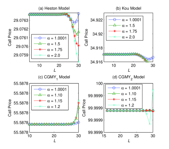
Figure 1: Damping parameter $\alpha$ and truncation parameter $L$ for Stable_Cos method.

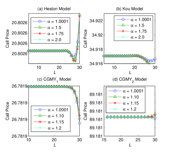
Figure 2: Damping parameter $\alpha$ and truncation parameter $L$ for Stable Cos method when $T=0.1$.

We compare our results with the Stable COS methods to two of Cos method, the direct Cos method and put-call parity Cos method in which the put price is calculated first, then by put-call parity, call price is obtained. We reference Stable_Cos to Stable COS method, Put-Call_Cos to put-call parity Cos method, and Direct_Cos to the direct Cos method. We have three kinds Cos methods.

3.1 Damping Factors and Truncation Range

In this subsection we consider the choice of the damping parameter $\alpha$ and truncation interval $[a,b]$. In order to illustrate the result numerically, we have chosen different values of $\alpha$ and $K=80$, $T=1$ for all models considered in this paper to generate the graphs given in Figure 1 by Stable Cos method. The reference value for the European option can be found from Table 5.

Figures 1 presents European call option values under different damping parameters $\alpha$ and range of Truncation parameters $L$. In Figure 1, the option values obtained by Stable Cos method. Figures 1 shows that option values are stable under $\alpha\in[1.0001,1.2]$ for all cases by Stable Cos method, and for most cases, $L\in[6,18]$ is reasonable except that the probability density function of the underlying is governed by fat tails. For fat tail cases, option values are stable under $L\in[17,25]$. Figures 3 and 4 show that such results are also robust for different $T$-values.

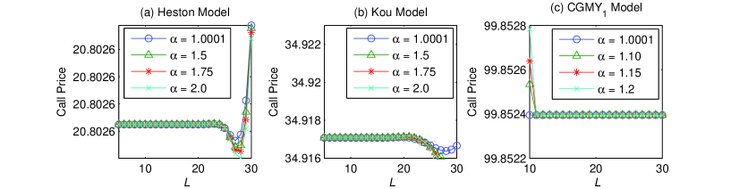
Figure 3: Damping parameter $\alpha$ and truncation parameter $L$ for Stable Cos method when $T=20$.

3.2 accuracy, efficiency and robustness of R_Cos

Now we examine the accuracy, efficiency and robustness of our robust Cos methods by a series of numerical examples. For further comparison, we use Carr-Madan method (Carr and Madan (1999)) to calculate call price for various models. In case of the Carr-Madan method, we use FFT method to calculate call prices with grid points $N=2^{16}$ and damping factor $\alpha=0.75$, and apply cubic interpolation to obtain desirable price. Moreover, we also use Fourier transform method (FTM) (Eberlein, Glau and Papapantoleon (2010)) to calculate call price. In later case, we use matlab built-in function quadgk to calculate the integrals with integral interval $[-5000,5000]$ and damping factor $\alpha=1.1$ for Heston, Kou, and CGMY_1 and damping factor $\alpha=1.015$ for CGMY_2.

In the experiments, the parameters of Cos methods is given by Table 4 where the values of $\alpha$, $L$ and $N$ are included for various models. These parameters are chosen such that same accuracy is obtained as as possible. Table 5 presents values of European call option to round ten decimals for a series of strike prices with $T=1$ using Stable Cos method, Put-call_Cos method, direct Cos method, FFT method and Fourier transform method. From Table 5, we can get the impression that the same accuracy is obtained by Stable Cos method and Put-call Cos method.

Table 4 The method parameters for calculating

call price by Three kinds of Cos methods

	Stable_Cos			Put-Call_Cos		Direct_Cos
Model	Damping	$L$	$N$	$L$	$N$	$L$	$N$
Heston	1.1	7	110	7	110	7	110
Kou	1.1	7	140	11	210	10	210
CGMY_1	1.001	10	50	10	50	13	80
CGMY_2	1.001	17	80	10	70

For efficiency comparison, we calculate the absolute errors of values of call option for a series of $N$ using four kinds of Cos methods with $K=100$ and $T=1$. The other method parameters is given by Table 4 and the reference values is given in Table 6. The computing results are plotted in Figure 4. As shown in Figure 4, the error convergence of Stable_Cos method is same as or superior to that of Put-Call_Cos method except CGMY_2, where error convergence of Stable_Cos is sightly inferior to that of Put-Call_Cos but still exponential.

The convergence results are not sensitive for different $T$-values. Figure 5 and 6 present error convergence results for CGMY_1 with $T=5$ and CGMY_2 with $T=0.1$ by Stable_Cos and Put-Call_Cos methods. As shown in Figure 5 and 6, error convergence results do not change much as $T$ changes.

Table 5 Values of Option Price in Various Models with $T=1$

Strike	Stable_Cos	Put-Call_Cos	Direct_Cos	FTM	FFT
Heston Model
80	29.0763658809	29.0763658809	29.0763658809	29.0763658809	29.0761596018
85	25.3190242256	25.3190242256	25.3190242256	25.3190242256	25.3182564563
90	21.8125703138	21.8125703138	21.8125703138	21.8125703138	21.8118590739
95	18.5866087601	18.5866087601	18.5866087601	18.5866087601	18.5863467950
100	15.6621055646	15.6621055646	15.6621055646	15.6621055646	15.6621055646
105	13.0502592738	13.0502592738	13.0502592738	13.0502592738	13.0499484651
110	10.7523654075	10.7523654075	10.7523654075	10.7523654075	10.7513381775
115	8.7605509099	8.7605509099	8.7605509099	8.7605509099	8.7590733973
120	7.0591610639	7.0591610639	7.0591610639	7.0591610639	7.0581882812
Kou Model
80	34.9170704483	34.9170704483	34.9170704483	34.9170704483	34.9170564801
85	31.9123200707	31.9123200707	31.9123200707	31.9123200707	31.9123052075
90	29.0794136987	29.0794136987	29.0794136987	29.0794136987	29.0793943989
95	26.4197703718	26.4197703718	26.4197703718	26.4197703718	26.4197774446
100	23.9335400091	23.9335400091	23.9335400091	23.9335400091	23.9335400091
105	21.6196765651	21.6196765651	21.6196765651	21.6196765651	21.6196851589
110	19.4760004471	19.4760004471	19.4760004471	19.4760004471	19.4759675797
115	17.4992412865	17.4992412865	17.4992412865	17.4992412865	17.4992369744
120	15.6850612076	15.6850612076	15.6850612077	15.6850612076	15.6850931891
CGMY_1
80	55.5877500641	55.5877500641	55.5877500089	55.5877500641	55.5877433925
85	54.0282287092	54.0282287092	54.0282286548	54.0282287092	54.0281877377
90	52.5459973200	52.5459973200	52.5459972649	52.5459973200	52.5459627032
95	51.1352855665	51.1352855665	51.1352855100	51.1352855665	51.1352741113
100	49.7909054685	49.7909054685	49.7909054141	49.7909054685	49.7909054685
105	48.5081777104	48.5081777104	48.5081776544	48.5081777104	48.5081662419
110	47.2828690189	47.2828690189	47.2828689625	47.2828690189	47.2828329497
115	46.1111387169	46.1111387169	46.1111386614	46.1111387169	46.1110877016
120	44.9894929189	44.9894929189	44.9894928638	44.9894929189	44.9894576019
CGMY_2
80	99.9999155240	99.9999155240		99.9999155240	99.9999155240
85	99.9999129093	99.9999129092		99.9999129092	99.9999129093
90	99.9999103728	99.9999103728		99.9999103728	99.9999103728
95	99.9999079083	99.9999079083		99.9999079082	99.9999079083
100	99.9999055101	99.9999055101		99.9999055100	99.9999055101
105	99.9999031733	99.9999031732		99.9999031732	99.9999031733
110	99.9999008935	99.9999008935		99.9999008935	99.9999008935
115	99.9998986670	99.9998986669		99.9998986669	99.9998986670
120	99.9998964902	99.9998964902		99.9998964901	99.9998964902

Note: FTM reference to Fourier transform method (Eberlein, Glau and Papapantoleon (2010)).

Finally, we consider the robustness of our methods. For given the method parameters in Table 4, we calculate values of call price by Stable_Cos method and Put-Call_Cos method for range of $L$-values $L$. The computing results are shown in Figure 7. From Figure 7, we find that size of the integration interval is almost same for two methods, so our method has same robustness as Put-Call_Cos method.

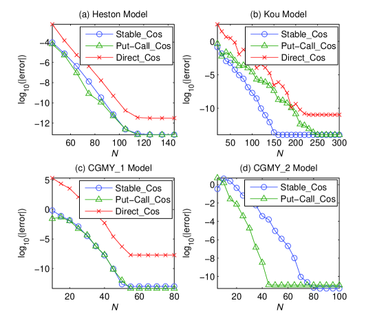
Figure 4: Convergence of Stable Cos method, Put-Call Cos method and Direct Cos method.

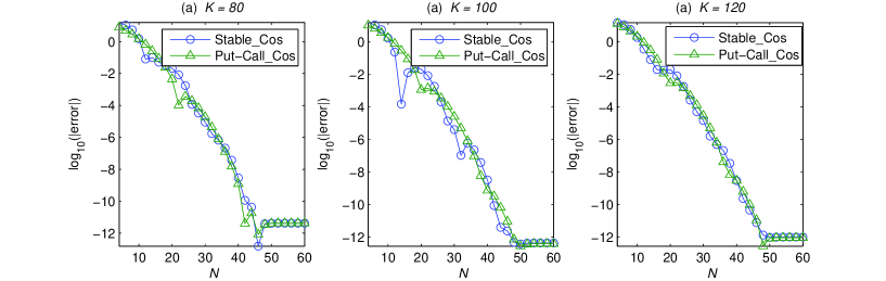
Figure 5: Convergence of Stable_Cos method and Put-Call_Cos method for CGMY_1 with $T=5$.

Table 6 The reference values for calculate the absolute errors

for four kinds of Cos methods with $K=100$ and $T=1$

Model	reference values
Heston	15.6621055645751
Kou	23.9335400090856
CGMY_1	49.7909054685239
CGMY_2	99.9999055100654

Note: The reference values are obtained by Put-Call_Cos with $N=60000$.

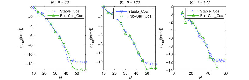
Figure 6: Error convergence of Stable_Cos method and Put-Call_Cos method for CGMY_2 with $T=0.1$.

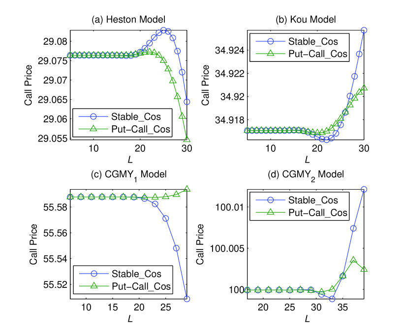
Figure 7: Comparison of $L$-values by Stable_Cos method and Put-Call_Cos method.

4 Conclusions

In this paper, we present a robust pricing of call options based on Fourier cosine series expansion. The robust COS method exhibits an exponential convergence in $N$ for density functions in $C^{\infty}[a,b]$ and an impressive computational speed. With a limited number, $N$, of Fourier cosine coefficients, it produces highly accurate results. We also present error analysis for this method, showing that error convergence is easily obtained. Robust pricing, insensitive of the choice of the size of the integration range is achieved for call options. The accuracy, efficiency and robustness of our robust Cos methods are demonstrated by error analysis, as well as by a series of numerical examples, including Heston stochastic volatility model, Kou jump-diffusion model, and CGMY model.

References

- [1] P. Carr, H. Geman, D. B. Madan, and M. Yor. The fine structure of asset returns: An empirical investigation. Journal of Business, 75(2):305-332, 2002.
- [2] P. Carr and D. B. Madan. Option valuation using Fast Fourier Transformation. Journal of Computational Finance, 2: 61-73,1999.
- [3] E. Eberlein, K. Glau, and A. Papapantoleon. Analysis of Fourier transform valuation formulas and applications. Applied Mathematical Finance, 17:211-240, 2010.
- [4] F. Fang and C. W. Oosterlee. A Fourier-based valuation method for bermudan and barrier options under Heston’s model. SIAM Journal of Financial Mathematics, 2(1):439-463, 2011.
- [5] F. Fang and C. W. Oosterlee. A novel pricing method for european options based on fourier-cosine series expansions. SIAM Journal on Scientific Computing, 31(2):826-848, 2008.
- [6] F. Fang and C. W. Oosterlee. Pricing early-exercise and discrete barrier options by fourier-cosine series expansions. Numerische Mathematik, 114:27-62, 2009.
- [7] L. Feng and V. Linetsky, Pricing discretely monitored barrier options and defaultable bonds in Lévy process models: a fast Heston transform approach. Mathematical Finance, 18, 2008.
- [8] T. R. Hurd, Zhuowei Zhou A Fourier transform method for spread option pricing, SIAM Journal of Financial Mathematics, 1, 142-157, 2010.
- [9] R. Lord, F. Fang, F. Bervoetsand C. W. Oosterlee, A fast and accurate FFT-based method for pricing early-exercise options under Lévy processes. SIAM Journal on Scientific Computing, 30, 2008.
- [10] B. Zhang and C. W. Oosterlee, Fourier cosine expansions and put call relations for Bermudan options. Numerical Methods in Finance, 325-352, 2011.
- [11] B. Zhang and C. W. Oosterlee. Efficient pricing of European-style Asian options under exponetial Lévy processes based on Fourier cosine expansions. SIAM Journal of Financial Mathematics, 4 (1):399-426, 2013.