Synthesis of Ultra-Wideband TEM Horn with Inhomogeneous Dielectric Medium

Abstract

There were proposed new formulas for the dielectric medium permittivity distribution along spatial coordinates in the space between a linear TEM-horn’s leafs, which were obtained according to the rules of geometric optics in the assumption of the phase center being lumped or distributed. The formulas has been checked by FDTD simulation of an ultra-wideband signal excitation; two cases were studied—when dielectric medium is present, and absent. For these both cases, there was obtained voltage steady-wave ratio, as well as radiation patterns at a set of frequencies up to 20 GHz; the results comparison was performed.

1 Introduction

These days TEM-horns of various types are widely used as antennas in ultra-wideband (UWB) radiolocation and communication; TEM-horns earned their popularity for having wide range of operational frequencies, while being extremely easy for manufacturing. Unfortunately, these antennas have a number of drawbacks too; for example, they must have relatively large electric size to radiate signals efficiently and may have low-gain frequency gaps. These drawbacks can be partially worked around by carefully choosing antenna size and shape [1, 2, 3, 4, 5]; moreover, it is possible to make horn operational frequency range even wider, usually at the cost of further antenna size increasing [6].

There is another approach for improving TEM-horns’ gain and patterns which is based on combining antennas with dielectric objects. These objects usually are complex-shaped lens manufactured from a solid material which are placed at aperture plane or beyond it [7, 8]; while improving gain and patterns, these techniques have a common downside of increasing energy reflection back to feeding line and, hence, increasing voltage steady-wave ratio (VSWR) at higher frequencies.

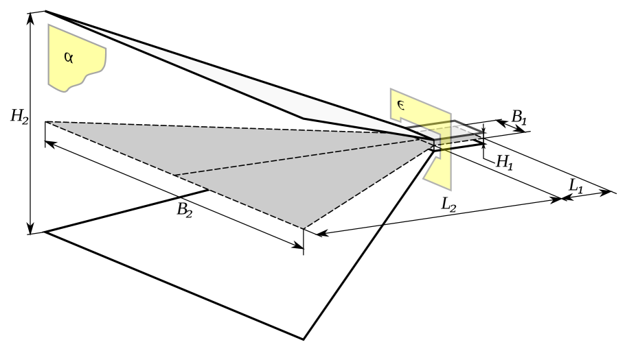
Figure 1: TEM horn antenna of the interest, with size markers shown. Here $\alpha$ is the aperture plane, $\epsilon$ is the excitation plane.

However, there is way to improve horn’s directivity without sacrificing VSWR level. Its essence is filling the space between horn leafs by dielectric medium with spatially varying permittivity; manufacturing of such filling objects was a major technological problem in near past, which can be successfully solved in present time using a number of techniques, including, but not limited to, 3D printing [9, 10]. For example, Molina and Hasselbarth [10] accompanied a planar slot radiator by a dielectric lense created by layer-by-layer backing a mixture of alumina ceramic powder and microscopic hollow glass spheres.

In this work, for a given TEM horn with flat trapezoidal leafs (see Fig. 1 for its schematic view) we (a) derive dielectric filling permittivity distribution from geometric optics model of radiation process, and (b) use time-domain computer simulation of ultra-short pulse propagation to check whether adding this filling actually improves horn characteristics.

2 Wavefront planarization

Let’s assume for the rest of the paper that UWB signals propagate through the space like they are beams of light. Obviously, this assumption is quite strong for frequency order of tens gigahertz, but it lets us derive simple, but useful material distributions. This approach is not uncommon in antenna design [11, 12], either.

In the following subsections we present two similarly obtained distribution formulas. For the first one, we assumed that the whole electromagnetic wave was emitted from the single point (we call it a lumped phase center in this paper); for the second one, we uniformly stretched that phase center across horn’s excitation plane to form a distributed phase center.

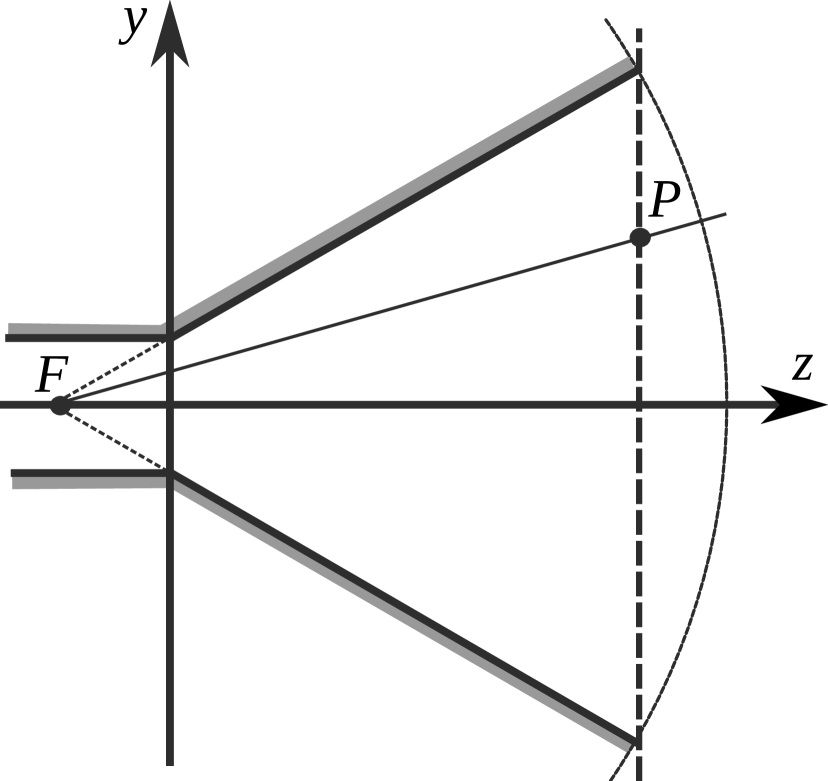
(a) lumped phase center

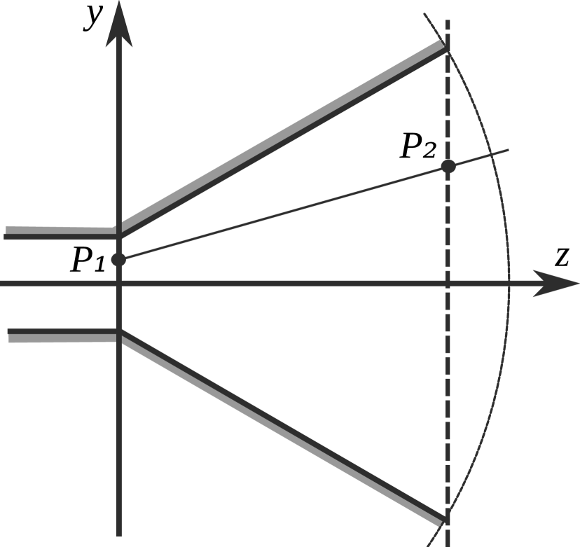
(b) distributed phase center

Figure 2: To the wavefront planarization procedures.

(a) no filling

(b) lumped phase center

(c) distributed phase center

Figure 3: Electric field magnitude in horn’s horizontal symmetry plane at 15 $\mathrm{GHz}$ (time-domain simulation).

2.1 Lumped phase center

Let’s choose a system of Cartesian coordinates such that $x$ axis is horizontal, $y$ axis is vertical, and $z$ is TEM-horn’s main direction (as shown in Fig. 2(a)); and put the origin at the point where the horn’s symmetry axes intersect the excitation plane. Also consider the point $F$ which is the midpoint of the line formed by horn leafs’ continuations intersection; let this $F$ be the lumped phase center.

If electromagnetic beams are simultaneously emitted from $F$, then after a certain amount of time they form a spherical wavefront. The idea is to slow down central beams by increasing dielectric permittivity along their trajectories, and, hence, turn the spherical wavefront into a plane.

Let $R_{\text{max}}$ be the longest possible straight path from $F$ to the aperture rectangle as $R_{\text{max}}$, which is the line pointing to a leaf’s trapeze apex. Since that path is the longest, the material along it must have the lowest dielectric permittivity among all beam paths; call it $\varepsilon_{\text{min}}$. It is safe to assume that $\varepsilon_{\text{min}}=1$, hence

$$t_{\text{max}}=\frac{R_{\text{max}}}{c}$$

is the time required for a beam to travel along the $R_{\text{max}}$ path, where $c$ is the speed of light in free space.

Let’s now consider a beam propagating in arbitrary direction inside the horn. Let $R$ be the distance between $F$ and the point $P$ where the beam intersects the aperture plane $\alpha$, so the time required for the beam to travel to that point is

$$t=\frac{R}{v},$$

where $v$ is the speed of electromagnetic wave in the dielectric material located along the path.

For the $R_{\text{max}}$-beam and $R$-beam to reach the horn exit plane simultaneously, the following condition must be met:

$$\frac{R_{\text{max}}}{c}=\frac{R}{v}.$$

Taking into account that $\varepsilon=(c/v)^{2}$, the following expression for the dielectric permittivity inside the horn can be obtained:

$$\varepsilon=\frac{R^{2}_{\text{max}}}{R^{2}}.$$ (1)

In the coordinate system we introduced above, it can be stated that

$$R^{2}_{\text{max}} =\frac{1}{4}\left(B_{2}^{2}+H_{2}^{2}\right)+\left(L_{2}+l\right)^{2},$$

$$R^{2} =x^{2}+y^{2}+\left(L_{2}+l\right)^{2},$$

where $l$ is the distance between $F$ and the excitation plane, $x$ and $y$ are the coordinates of a point $P$, $|x|\leq B_{2}/2$, $|y|\leq H_{2}/2$. If we substitute the above expression into equation (1), we get the following expression:

$$\varepsilon=\frac{\frac{1}{4}\left(B_{2}^{2}+H_{2}^{2}\right)+\left(L_{2}+l\right)^{2}}{x^{2}+y^{2}+\left(L_{2}+l\right)^{2}}.$$ (2)

Equation (2) gives us a formula of material distribution along straight lines connecting $F$ and each point at the aperture plane. It can be also rewritten as the $\varepsilon(\theta)\propto\cos^{2}\theta$ dependence, where $\theta$ is the angle between the beam and the horn’s main direction.

2.2 Distributed phase center

Despite the above section’s approach has proven itself to work in practice, its propagation model is simplistic and cannot reflect reality very well. Let’s elaborate the model to make it more adequate.

Computer simulation shows (Fig. 3(a)) that TEM horn does not emit waves from just a single point; instead, the irradiation process involves the whole excitation plane. This means that the phase center should not be though as a lumped entity, but as a continuum of phase centers distributed on the excitation plane between horn leafs. So, let’s modify the formula (2) to convert lumped phase center into distributed.

As in the previous case, we continue to think about the wavefront as a set of beams, but now these beams are not required to have a common origin (former point $F$). Instead, let each beam start from the point $P_{1}=(x_{1},y_{1})$ at the excitation plane and intersect the aperture plane at the point $P_{2}=(x_{2},y_{2})$. Let’s additionally require the following restriction to satisfy:

$$\frac{x_{1}}{B_{1}}=\frac{x_{2}}{B_{2}},\quad\frac{y_{1}}{H_{1}}=\frac{y_{2}}{H_{2}}.$$ (3)

In these new circumstances, $R$ and $R_{\text{max}}$ values can be obtained as

$$R^{2}_{\text{max}} =\frac{1}{4}\left[\left(B_{2}-B_{1}\right)^{2}+\left(H_{2}-H_{1}\right)^{2}\right]+\left(L_{2}-L_{1}\right)^{2},$$

$$R^{2} =\left(x_{2}-x_{1}\right)^{2}+\left(y_{2}-y_{1}\right)^{2}+\left(L_{2}-L_{1}\right)^{2}.$$

If we substitute the above expressions into equation (1) taking into account that $x_{1}=\frac{B_{1}}{B_{2}}x_{2}$ and $y_{1}=\frac{H_{1}}{H_{2}}y_{2}$, when the final formula will be

$$\varepsilon=\frac{\frac{1}{4}\left[\left(B_{2}-B_{1}\right)^{2}+\left(H_{2}-H_{1}\right)^{2}\right]+\left(L_{2}-L_{1}\right)^{2}}{\left(1-\frac{B_{1}}{B_{2}}\right)^{2}x_{2}^{2}+\left(1-\frac{H_{1}}{H_{2}}\right)^{2}y_{2}^{2}+\left(L_{2}-L_{1}\right)^{2}}.$$ (4)

3 Computer simulation model

In order to check the proposed material distributions, we made their digital models, suitable for finite-difference time-domain (FDTD) [13] simulation. This model included a simple TEM horn (Fig. 1) with a strip feeding line; the dimensions were chosen as follows:

$$\begin{array}[]{ll}L_{1}=30\,\mathrm{mm},&L_{2}=30\,\mathrm{mm}\\ B_{1}=10\,\mathrm{mm},&B_{2}=50\,\mathrm{mm}\\ H_{1}=2\,\mathrm{mm},&H_{2}=50\,\mathrm{mm}\\ \end{array}$$

In this model, all antenna and feeder surfaces were approximated by thin perfect electric conductors. The whole problem’s geometry was fit into $68\,\mathrm{mm}\times 57\,\mathrm{mm}\times 63\,\mathrm{mm}$ computational domain and split into $151\times 135\times 137$ cuboid Yee cells. To prevent radiated signal from reflecting back into computational domain, four-layer convolutional perfectly matched layer (PML) boundary condition [14] was applied to domain edges (each having 5 $\mathrm{mm}$ as the minimum distance to the nearest conducting surface).

4 Obtained results

After simulation run, we obtained horizontal-plane antenna patterns at 5, 10, 15, and 20 $\mathrm{GHz}$ frequencies, as well as the feeding line S-parameters. Additionally, images of electric field were constructed; they were already presented in Fig. 3

Figures 3(b) and 3(c) demonstrate that both lumped and distributed phase center approaches make wavefront a flatter shape (compared to normal medium, Fig. 3(a)), though, not a perfect plane. However, in the case of the distributed phase center, more of peripheral aperture is involved in signal formation, thus increasing antenna’s effective area.

Obtained patterns are presented in Fig. 4. It can be seen that the presence of dielectric filling (with either lumped or distributed phase center) improves directional selectivity of antenna; more specifically, filled antennas have higher gains at all considered frequencies (Fig. 5(a)), as well as narrower main lobes. This improvement is more significant for the cases of 15 and 20 $\mathrm{GHz}$ than for 5 and 10 $\mathrm{GHz}$. Moreover, adding dielectric filling prevented main lobe from splitting at 20 $\mathrm{GHz}$, which we consider a notable practical result.

Figure 5(b) shows VSWR frequency dependence which was calculated from S-parameters obtained after the simulation run. It shows that the above said gain and directivity improvements did not compromised antenna matching.

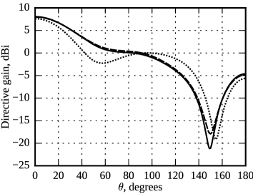
(a) $f=5\,\mathrm{GHz}$

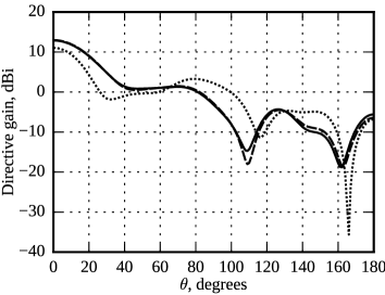
(b) $f=10\,\mathrm{GHz}$

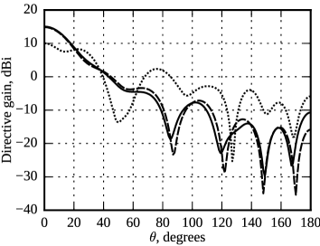
(c) $f=15\,\mathrm{GHz}$

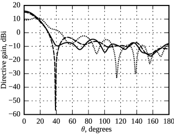
(d) $f=20\,\mathrm{GHz}$

Figure 4: Antenna patterns in the horizontal symmentry plane, where $\theta$ is the angle betwen the direction and $z$ axis.

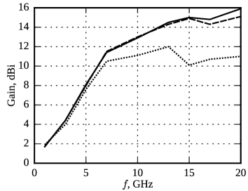
(a) gain

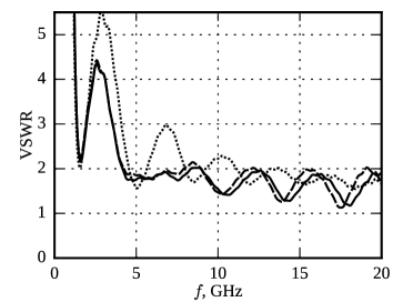
(b) VSWR

Figure 5: TEM horn frequency parameters.

5 Conclusion

This paper presented two similar, but different formulas for filling TEM-horns by inhomogeneous dielectric medium. They were obtained in the assumption of light-like propagation of the UWB signal. Though this assumption is quite unrealistic, computer simulation confirmed that employing these formulas for generating dielectric filling significantly increases horn’s gain and directional selectivity without impairing antenna matching.

Despite the antenna being studied was linear TEM-horn, the same approach can potentially be applied to more complex-shaped horns by, for example, subdividing this complex shape into a number of short linear intervals.

References

- [1] Kyungho Chung, S. Pyun and Jaehoon Choi “Design of an ultrawide-band TEM horn antenna with a microstrip-type balun” In IEEE Trans. Antennas Propag. 53.10 Institute of ElectricalElectronics Engineers (IEEE), 2005, pp. 3410–3413 DOI: 10.1109/tap.2005.856396
- [2] A. M. Bobreshov, I. I. Meshcheryakov and G. I. Uskov “Optimization of the flare angle of a TEM horn for efficient radiation of ultrashort pulses” In Journal of Communications Technology and Electronics 57.3 Pleiades Publishing Ltd, 2012, pp. 291–295 DOI: 10.1134/s1064226912020027
- [3] A. M. Bobreshov, I. I. Meshcheryakov and G. K. Uskov “Optimization of the geometry of a TEM-horn for radiation of ultrashort pulses used as an element of an antenna array with controlled position of the main lobe” In Journal of Communications Technology and Electronics 58.3 Pleiades Publishing Ltd, 2013, pp. 203–207 DOI: 10.1134/s1064226913030042
- [4] Yong-Guang Chen, Yun Wang and Qing-Guo Wang “A New Type of TEM Horn Antenna for High-Altitude Electromagnetic Pulse Simulator” In IEEE Antennas Wireless Propag. Lett. 12 Institute of ElectricalElectronics Engineers (IEEE), 2013, pp. 1021–1024 DOI: 10.1109/lawp.2013.2278202
- [5] Ali Mehrdadian and Keyvan Forooraghi “Design and Fabrication of a Novel Ultrawideband Combined Antenna” In IEEE Antennas Wireless Propag. Lett. 13 Institute of ElectricalElectronics Engineers (IEEE), 2014, pp. 95–98 DOI: 10.1109/lawp.2013.2296559
- [6] R.T. Lee and G.S. Smith “A design study for the basic TEM horn antenna” In IEEE Antennas Propag. Mag. 46.1 Institute of ElectricalElectronics Engineers (IEEE), 2004, pp. 86–92 DOI: 10.1109/map.2004.1296150
- [7] Eric L. Holzman “A highly compact 60-GHz lens-corrected conical horn antenna” In IEEE Antennas Wireless Propag. Lett. 3.1 Institute of ElectricalElectronics Engineers (IEEE), 2004, pp. 280–282 DOI: 10.1109/lawp.2004.831082
- [8] N. A. Efimova, V. A. Kaloshin and E. A. Skorodumova “Analysis of a horn-lens TEM antenna” In Journal of Communications Technology and Electronics 57.9 Pleiades Publishing Ltd, 2012, pp. 1031–1038 DOI: 10.1134/s1064226912090045
- [9] Min Liang et al. “A 3-D Luneburg Lens Antenna Fabricated by Polymer Jetting Rapid Prototyping” In IEEE Trans. Antennas Propag. 62.4 Institute of ElectricalElectronics Engineers (IEEE), 2014, pp. 1799–1807 DOI: 10.1109/tap.2013.2297165
- [10] Hernan Barba Molina and Jan Hesselbarth “Microwave dielectric stepped-index flat lens antenna” In International Journal of Microwave and Wireless Technologies Cambridge University Press (CUP), 2016 DOI: 10.1017/s1759078716001124
- [11] Aki Karttunen, Juha Ala-Laurinaho, Ronan Sauleau and Antti V Raisanen “Reduction of internal reflections in integrated lens antennas for beam-steering” In Progress In Electromagnetics Research 134 EMW Publishing, 2013, pp. 63–78
- [12] Iman Aghanejad, Habibollah Abiri and Alireza Yahaghi “Design of High-Gain Lens Antenna by Gradient-Index Metamaterials Using Transformation Optics” In IEEE Trans. Antennas Propag. 60.9 Institute of ElectricalElectronics Engineers (IEEE), 2012, pp. 4074–4081 DOI: 10.1109/tap.2012.2207051
- [13] A. Taflove “Computational electrodynamics: the finite-difference time-domain method”, Antennas and Propagation Library Artech House, 1995
- [14] J.-P. Berenger “Perfectly matched layer for the FDTD solution of wave-structure interaction problems” In IEEE Trans. Antennas Propag. 44.1, 1996, pp. 110–117 DOI: 10.1109/8.477535
- [15] Rudolf Karl Luneburg “Mathematical Theory of Optics” In Mathematical Theory of Optics by R. K. Luneburg Berkeley, CA: University of California Press, 1964 Berkeley & Los Angeles:: University of California Press, 1964
- [16] A. Rolland et al. “Lens-Corrected Axis-Symmetrical Shaped Horn Antenna in Metallized Foam With Improved Bandwidth” In IEEE Antennas Wireless Propag. Lett. 11 Institute of ElectricalElectronics Engineers (IEEE), 2012, pp. 57–60 DOI: 10.1109/lawp.2011.2182596