Phase Transition of Charged-AdS Black Holes and Quasinormal Modes : a Time Domain Analysis

Abstract

In this work we use the quasinormal mode of a massless scalar perturbation to probe the phase transition of the charged-AdS black hole in time profile. The signature of the critical behavior of this black hole solution is detected in the isobaric process. This paper is a natural extension of [1, 2] to the time domain analysis. More precisely, our study shows a clear signal in term of the damping rate and the oscillation frequencies of the scalar field perturbation. We conclude that the quasinormal modes can be an efficient tool to detect the signature of thermodynamic phase transition in the isobaric process far from the critical temperature, but fail to disclose this signature at the critical temperature.

Keywords: Quasinormal modes, $AdS$ black holes, Phase transitions.

1 Introduction

The main motivation behind the study of black holes in the asymptotically AdS spacetime is provided by the gauge/gravity correspondence [3, 4], which is a powerful tool applied to a broad variety of research areas like theoretical particle physics, string theory, QCD, nuclear physics and condensed-matter physics [5, 6, 7, 8]. In this context [3, 9, 10, 11], the black hole is identified with an approximately thermal state in the field theory, and the decay of the test field corresponds to the decay of the perturbation of the state. In this way, the understanding of asymptotically AdS black hole is a crucial step towards a more insight into the above conjecture.

Recently, a particular emphasis has been dedicated to the study of phases transitions of the black holes in AdS space [12, 13] that consolidates the analogy between the critical Van der Waals gas behavior and the charged AdS black hole one [14, 15, 16, 17, 18, 19, 1], using several approaches based on mathematical methods. Especially the quasinormal modes (QNM) [1, 2, 20] which has been proved efficient to disclose the thermodynamic phase transition. More precisely, in [1, 2, 20] the authors foundd a drastic change in the slopes of the quasinormal frequencies in the small (SBH) and large (LBH) black holes near the critical point where the Van der Waals like thermodynamic phase transition occurs for different spacetime dimensions and gravity configuration using the frequencies domain analysis. Another important motivation is related to new detection of the gravitational waves whose recent observation is an important landmark in the gravitational waves astronomy [21, 22].

The aim of the work is to extend this technical method tothe time-domain analysis and show a correspondence between the thermodynamical phase transition and the time evolution of the wave function.

The layout of the letter is as follows: in section 2 we briefly review some aspects of the phase transition in the extended phase space in the temperature-horizon radius plan. In section 3 we present the master equation of the evolution of a massless scalar field in the four dimensional RN-AdS background as well as the numerical procedures used to solve Section $4$ is devoted to establish a link between the damping rate, the oscillation number of the scalar field and the small/large black hole phase transition and to show that the behavior discussed in our previous work [1] is well reproduced. In the last section, we will draw our conclusions.

2 Critical behavior of $\text{RN-AdS}_{4}$ black holes

Let us recall some aspects of the system to be studied. Reissner Nordstrom AdS black hole is solution of Einstein-Maxwell theory with negative cosmological constant in four dimensions which described by the following action

$$I_{EM}=-\frac{1}{16\pi G_{4}}\int_{M}d^{4}x\sqrt{-g}\Bigl{(}\mathcal{R}-F^{2}+\frac{6}{R^{2}}\Bigr{)}\,.$$ (1)

where $\mathcal{R}$ is the Ricci scalar, $F_{\mu\nu}$ is the strength of electromagnetic field and $R$ is the curvature radius of AdS space. We have assumed the universal gravitational constant $G_{4}=~{}1$. Solving Einstein equations yields to the following the static spherical metric

$$ds^{2}=-fdt^{2}+\frac{dr^{2}}{f}+r^{2}d\omega_{2}^{2},$$ (2)

with,

$$f=1-\frac{2M}{r}+\frac{Q^{2}}{r^{2}}+\frac{r^{2}}{R^{2}}\,,$$ (3)

and $d\omega_{2}^{2}$ stands for the metric of a four dimensional unit sphere. The two parameters $M$ and $Q$ are the mass and the charge of the black hole respectively. The Hawking temperature reads as

$$T=\left.\frac{f^{\prime}(r)}{4\pi}\right|_{r=r_{H}}=\frac{1}{4\pi r_{H}}\Bigl{(}1-\frac{Q^{2}}{r_{H}^{2}}+\frac{3r_{H}^{2}}{R^{2}}\Bigr{)}\,,$$ (4)

where the position of the black hole event horizon $r_{H}$ is determined by solving the equation $f(r)|_{r=r_{H}}=0$ and choosing the largest real positive root. The electric potential $\Phi$ measured at infinity with respect to the horizon while the black hole entropy $S$ are given by the following form

$$\Phi = \frac{Q}{r_{H}}\,,$$ (5)

$$S = \pi r_{H}^{2}\,.$$ (6)

Now, we reconsider the extended phase space by defining a thermodynamical pressure proportional to cosmological constant and its corresponding conjugate quantity as the volume, using the following equation

$$P=-\frac{\Lambda}{8\pi}=\frac{1}{8\pi R^{2}}\,,$$ (7)

In this context the mass is identified with the enthalpy [24, 12], the first law of black hole thermodynamics becomes,

$$dM=TdS+\Phi dQ+VdP\,,$$ (8)

where the thermodynamic volume can be defined as

$$V=\left.\frac{\partial M}{\partial P}\right|_{S,Q}.$$ (9)

To the Gibbs free energy $G=M-TS$, for fixed charge, it reads as [23]

$$G=G(P,T)=\!\frac{1}{4}\biggl{(}\!r_{H}-\frac{8\pi Pr_{H}^{3}}{3}+\frac{3Q^{2}}{r_{H}}\biggl{)}.\ \$$ (10)

Now, having calculated the relevant thermodynamic quantities, we turn now to the analysis of the corresponding phase transition. For this, we plot in figure 1 the variation of the Hawking temperature and the Gibbs free energy as a function of the horizon radius given by Eq. (4) and Eq. (10). We set the charge $Q$ to $1$ for all the rest of this letter.

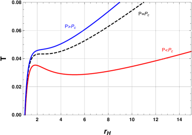
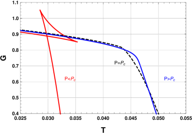
Figure 1: Left: Isobaric curves of RN-AdS black hole with different pressure. Right: The Gibbs free energy function of the temperature. For each panel from bottom to top the corresponding pressure are $0.4P_{c}$ (red), $P_{c}$ (Dashed Black), $1.2P_{c}$ (Blue)

As discussed in [12, 13], there exists some critical behavior. In particular the first order phase transition in the $P-V$ diagram signaled by the “swallow tail” shown in the right panel of figure 1. This behavior is similar to the Van der Waals one. We perform a similar calculation on the $T-r_{H}$ plane by fixing the pressure. The coordinates of the critical point can be obtained by solving the following system of equations

$$\frac{\partial^{2}T}{\partial r_{H}^{2}}=\frac{\partial T}{\partial r_{H}}=0,$$ (11)

which give rise to the following critical pressure, critical radius and the critical temperature

$$P_{c}=\frac{1}{96\pi},\quad r_{H_{c}}=\sqrt{6},\quad\text{and }\;T_{c}=\frac{1}{3\sqrt{6}\pi}.$$ (12)

After having briefly introduced the main thermodynamical quantities and related phase transition, we will study in the next section the late–time decay of a scalar perturbation around a charged AdS black holes in four dimensional spacetime.

3 Master equation and numerical method

We start by considering the evolution of a massless scalar field in charged AdS black hole background, satisfying the Klein-Gordon differential equation

$$\frac{1}{\sqrt{-g}}\partial_{\mu}\left(\sqrt{-g}g^{\mu\nu}\partial_{\nu}\Phi\right)=0,$$ (13)

then,we decompose the scalar field as

$$\Phi=\sum_{\ell,m}r^{-1}\psi(t,r)Y_{\ell,m}(\theta,\phi),$$ (14)

to separate the radial and angular variables. The radial equation is giving by [25, 26]

$$-\frac{\partial^{2}\psi}{\partial^{2}t}+f\frac{\partial}{\partial r}\left(f\frac{\partial\psi}{\partial r}\right)=V_{\ell}\psi,$$ (15)

where the effective potential $V_{\ell}$ has the form [35, 31]

$$V_{\ell}=\left[\frac{\ell(\ell+1)}{r^{2}}+\frac{1}{r}\frac{\partial f}{\partial r}\right]f,$$ (16)

where $\ell$ is the angular quantum number. In this letter we will focus only on the case $\ell=0$ and we tortoise coordinate defined by $r^{*}=\int\frac{dr}{f}$ (up to an arbitrary constant). If we take $r^{*}\left(r\rightarrow\infty\right)~{}=~{}0$, the analytic form of $r^{*}$ in function of $r$ is giving by [28, 34, 36]

$$r^{*}=\frac{\log\left(r-r_{H}\right)}{2\kappa_{H}}-\frac{\log\left(r-r_{C}\right)}{2\kappa_{C}}-A\log\left(T_{2}r+T_{1}+r^{2}\right)\\ +\frac{2(AT_{2}+B)}{\sqrt{4T_{1}-T_{2}^{2}}}\left[\tan^{-1}\left(\frac{T_{2}+2r}{\sqrt{4T_{1}-T_{2}^{2}}}\right)-\frac{\pi}{2}\right],$$ (17)

with
$T_{1}=r_{H}^{2}+r_{C}^{2}+r_{H}r_{C}+R^{2}$,  $\kappa_{H}=\frac{\left(r_{H}-r_{C}\right)\left(3r_{H}^{2}+r_{C}^{2}+2r_{H}r_{C}+R^{2}\right)}{2r_{H}^{2}R^{2}}$,   $A=\frac{R^{2}\left(r_{H}+r_{C}\right)\left(r_{H}^{2}+r_{C}^{2}+2r_{H}r_{C}+R^{2}\right)}{2\left(3r_{H}^{2}+r_{C}^{2}+2r_{H}r_{C}+R^{2}\right)\left(r_{H}^{2}+3r_{C}^{2}+2r_{H}r_{C}+R^{2}\right)}$,

$T_{2}=r_{H}+r_{C}$,                  $\kappa_{C}=\frac{\left(r_{H}-r_{C}\right)\left(r_{H}^{2}+3r_{C}^{2}+2r_{H}r_{C}+R^{2}\right)}{2r_{C}^{2}R^{2}}$    and  $B=\frac{R^{2}\left(r_{H}^{2}+r_{C}^{2}+R^{2}\right)\left(r_{H}^{2}+r_{C}^{2}+r_{H}r_{C}+R^{2}\right)}{\left(3r_{H}^{2}+r_{C}^{2}+2r_{H}r_{C}+R^{2}\right)\left(r_{H}^{2}+3r_{C}^{2}+2r_{H}r_{C}+R^{2}\right)}$.

$r_{C}$ and $r_{H}$ are Cauchy and event horizons respectively.

Therfore by using the tortoise coordinate, the Eq. (15) reduced to [30, 29, 25]

$$-\frac{\partial^{2}\psi}{\partial^{2}t}+\frac{\partial^{2}\psi}{\partial^{2}r^{*}}=V_{\ell}\psi.$$ (18)

In order to integrate the Eq. (15) we use the numerical method developed by Gundlach, Price and Pullin [27]. We start by introducing the null coordinates $u=t-r^{*}$ and $v=t+r^{*}$ to simplify the Eq. (18) which can be rewritten as two dimensional wave equation

$$-4\frac{\partial^{2}\psi\left(u,v\right)}{\partial u\partial v}=V_{\ell}\left(r\right)\psi\left(u,v\right).$$ (19)

Now the problem is reduced to the numerical integration of the Eq. (19), the values of the wave function $\psi$ can be found via the discretization method [27, 25, 29, 28], which we upon call Taylor’s theorem

$$\psi(N)=\psi(W)+\psi(E)-\frac{1}{8}\delta v\delta uV_{\ell}(\frac{v-u}{2})\left(\psi(W)+\psi(E)\right)\\ -\psi(S)+\mathcal{O}(\delta v\delta u),$$ (20)

where $S=(u,v)$, $W=(u+\delta u,v)$, $E=(u,v+\delta v)$ and $N=(u+\delta u,v+\delta v)$ form a null grid in the $v-u$ plane with horizontal step $\delta v$ and vertical step $\delta u$. In order to calculate the effective potential we need to invert numerically $r^{*}\left(r\right)=\frac{v-u}{2}$ to $r$ by using Eq. (17).

From Eq. (17) we see that $r^{*}$ is restricted within the range $-\infty<r^{*}<0$, which means that the only physical region in our problem is given by negative value of $r^{*}$ and only the case $v\leq u$ in our calculation has to be considered. In the purple line of figure 2, where $v=u$ we set $\psi=0$ since $r=\infty$ and $V_{\ell}$ diverge along this line [25]. Our objectif is evaluate the time evolution of the wave near the horizon, for this, we choose a sufficiently large $u_{max}$ by keeping $u_{max}>>v$, where $u_{max}$ is the maximum value of $u$ on the numerical grid, i.e when $u_{max}\rightarrow\infty$ the value of $r^{*}\rightarrow-\infty$, so $r$ tends to the horizon radius.

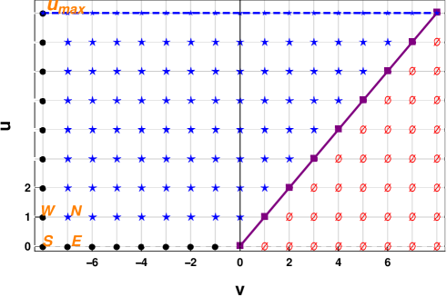
Figure 2: Diagram of the numerical grid

In figure 2, the black spots represent the initial grid points, the blue stars represent the grid points to be calculated, the red empty sets represent the forbidden region. The grid shows the iterative calculation up $u=u_{max}$ corresponding to the dashed blue line.

As in [29, 27], to solve the equation of perturbation under the assumption that the wave function is insensitive to the choice of the initial data, we impose the following conditions:

• Constant data on $v=v_{0}$, $\psi(u,v_{0})=\psi_{0}$.

• Gaussian distribution $\psi(u=u_{0},v)=A\exp\left(-\frac{\left(v-v_{c}\right)}{2\sigma^{2}}\right)$ on $u=u_{0}$.

In addition, the following parameters are fixed, $\psi_{0}=0$, $\sigma=3$, $A=1$, $v_{c}=0$, $u_{0}=0$, $v_{0}=-10$ and $\delta u=\delta v$.

After presenting the essential of the numerical method we turn our attention in the next section to the numerical simulation results, and the signature of the thermodynamical phase transitions in these results.

4 Time domain profile and isobaric phase transition

In our previous work [1] we found that the quasinormal mode frequencies are able to probe the small/large black hole phase transition in the isobaric process. In this section we will check this result by considering a time domain analysis.

To this end we computed the time evolution of the perturbation for 3 values of $r_{H}$ at the BH horizon by fixing the pressure at $P=0.00132$ ($P=0.4P_{c}$). The figure 3 and 4 correspond to the small and large black hole respectively. We found that for both SBH and LBH, the quasinormal ringing is quickly fading out with the increasing size of the BH.

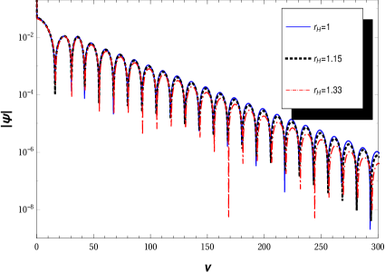
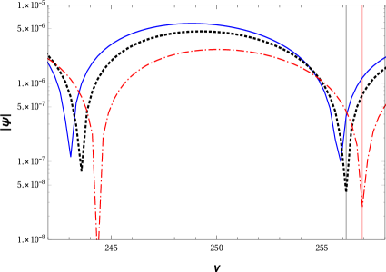
Figure 3: Left panel represent the time evolution of a scalar perturbation at the small $\text{AdS}_{4}$ black hole horizons (semi-log graph of $|\psi|$) for $r_{H}=1,1.15\ \text{and}\ 1.33$. Right panel is a zoom of the left one. The pressure is fixed at $P=0.4P_{c}$

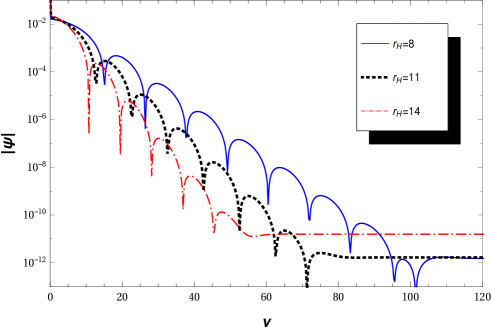
Figure 4: Time evolution of a scalar perturbation at the large $\text{AdS}_{4}$ black hole horizons (semi-log graph of $|\psi|$) for $r_{H}=8,11\ \text{and}\ 14$. The pressure is fixed at $P=0.4P_{c}$

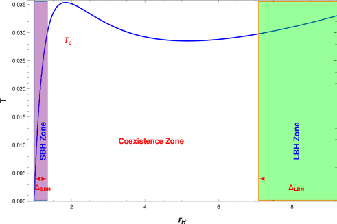
Figure 5: Isobaric $T-r_{H}$ diagram of charged $\text{AdS}_{4}$ black hole with $P=0.4P_{c}$. In general the range of $r_{H}$ in small black hole zone is very reduced $\Delta_{SBH}=0.353903$, contrariwise it is infinite in the large BH zone $\Delta_{LBH}=\infty$

Form figure 3 we can see that for the small black hole, when the horizon radius grows, the perturbation decays faster and the oscillation period increases. It is interesting to note that the increasing of oscillation frequencies is very slow, hence we cannot clearly distinguish the ringing of time evolution for each $r_{H}$. Indeed if we choose a pressure value far from the critical one, we will get very reduced range of the possible values of $r_{H}$ restricted by the extremal radius. One corresponds to $T=0$, while the other represents the maximum radius of SBH where $T=T_{c}$. As illustrative example with $P=0.4P_{c}$ one find $r_{H}(T=0)=0.984235$ and $r_{H_{SBH}}(T_{c})=1.33814$. On the other hand whatever the pressure of large black holes there is an infinity of possible values of $r_{H}$, as shown in figure 5.

From figure 4, for $\text{AdS}_{4}$ large black hole phase, the damping rate is monotonically increasing with the horizon radius $r_{H}$, but the oscillation period decrease with the increasing of $r_{H}$. The decay of the perturbation becomes faster for both small and large black holes with the growing of $r_{H}$, since the absorption ability of the black hole is enforced [2].

To make connexion with our previous work [1], we briefly present our results from frequency domain analysis.

Table 1 lists the frequencies of the quasinormal modes of the massless scalar perturbation around small and large black holes for the first order phase transition where the pressure is fixed at the value $P=0.4P_{c}$. In figure 6 we illustrate the quasinormal frequencies for SBH and LBH phases in $\omega_{r}-\omega_{im}$ plane, where the purple (blue) dots correspond to the results above (below) the horizontal line in table 1 respectively.

	$r_{H}$	$T$	$\omega_{r}$	$\omega_{im}$
SBH	1.	0.00265258	0.250222	-0.0348405
	1.15	0.0199248	0.249863	-0.0356006
	1.33	0.0295358	0.249177	-0.03761
LBH	8.	0.0310124	0.276141	-0.237695
	11.	0.0363529	0.31498	-0.327022
	14.	0.0427913	0.360997	-0.415881

Table 1: The quasinormal frequencies of the massless scalar perturbation as a function of the black holes temperature. The upper part, above the horizontal lines is for the small black hole phase while the lower part is for the large one. The pressure is fixed at $P=0.4P_{c}$

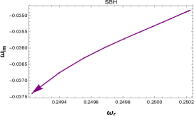
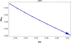
Figure 6: The behavior of the quasinormal modes for small and large black holes in the complex-$\omega$ plane. Increase of the black hole size is shown by the arrows. The pressure is fixed at $P=0.4P_{c}$

From table 1, we see that for small black hole process, the real part of the QNMs frequencies varies slightly, while the absolute value of the imaginary part decreases while in the large black hole phase the real part as well as the absolute value of the imaginary part of quasinormal frequencies increase. These observation can be driven from figure 6 where we see different slopes of the quasinormal frequencies in the massless scalar perturbations with different phases of the small and large black holes.

According to the discussion above, one can see that our results in the present work are in good agreement with [1, 2].As a summary: The damping rates for both SBH and LBH have the same behavior, the oscillation period decreases for the SBH while it increases for LBH. This result presents a consistent picture with those given by the quasi normal frequencies calculated in [1, 2, 20] which testify that the time domain analysis can be a useful tool to uncover a signature of the first order phase transition between SBH and LBH.

Besides, in our previous work [1] we also found that the critical ratio defined by $\chi=\frac{P}{P_{c}}$ affect the behavior of QNMs in the complex-$\omega$ plan, especially for small black hole. Probing the phase transition by the quasinormal modes in the frequency domain depends on the value of $\chi$. From figure 7, we see that for $\chi=0.9$ the $\omega$-complex plane does not show different slope in SBH and LBH phases. The change of slope (from the positive to negative slope) appears in the small black holes below the coexistence point. By approaching more and more the critical pressure, the QNMs become less effective to probe the phase transition and the slope change disappears at $\chi=1$.

Apart a preliminary numerical analysis proposed by Subhash Mahapatra in [20], we do not have yet an analytic formula or a powerful condition governing the slope in $\omega_{r}-\omega_{im}$ plane that allows QNMs to effectively probe the phase transition. The difficulty comes from from the master equation (15) which only depends on the parameters $P$ and $r_{H}$, regardless whether the black hole is large or small .

To compare the time domain with the results of frequency domain analysis, in figures 8 and 9, we have plotted the time evolution of a scalar perturbation for small and large black hole, with $\chi=0.9$. The left panel of figure 8 is zoom into a limited area of the right panel. Here, for the SBH, we have used optimal values of $r_{H}$ ($r_{H_{1}}$, $r_{H_{2}}$ and $r_{H_{3}}$) chosen from figure 7.

In figure 8 we can see that the problem of slope change persists. When crossing over from $r_{H_{1}}$ to $r_{H_{2}}$ the perturbation decays faster and becomes less oscillating. However, from $r_{H_{2}}$ to $r_{H_{3}}$ all the oscillations period increases and the scalar perturbation continues to decay faster. This is again consistent with the behavior of quasinormal frequencies shown in figure 7 since $\omega_{im}$ accounts for the damping time while $\omega_{r}$ reflects the oscillation period.

However, in the large black hole phase, we can see from figure 9 that the perturbation presents the same features as in the case $P=0.4P_{c}$. Now one can clearly figure out that the time evolution of a perturbation in figure 9 has a similar behavior as in green and red dash-dotted curves in figure 8. The evolution of wave function does not show different behavior (damping time and oscillation time) in small and large black hole phases near the critical temperature, hence the QNMs are not always an efficient tool to disclose the black hole phase transition.

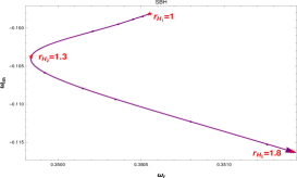
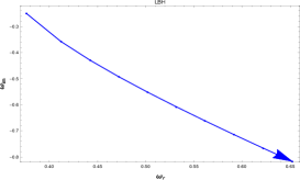
Figure 7: The behavior of the quasinormal modes for small and large black holes in the complex-$\omega$ plane. Increase of the black hole size is shown by the arrows. The pressure is fixed at $P=0.9P_{c}$

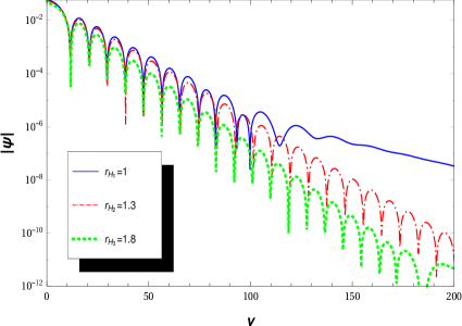
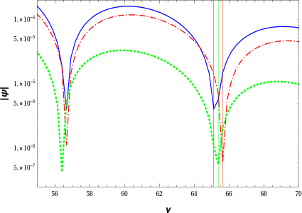
Figure 8: Left panel represent the time evolution of a scalar perturbation at the small $\text{AdS}_{4}$ black hole horizons (semi-log graph of $|\psi|$) for $r_{H}=1,1.3\ \text{and}\ 1.8$. Right panel is a zoom of the left one. The pressure is fixed at $P=0.9P_{c}$

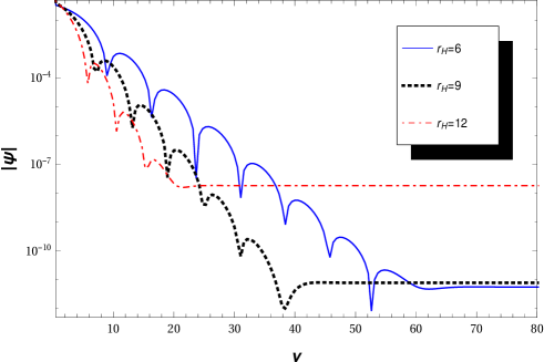
Figure 9: Time evolution of a scalar perturbation at the large $\text{AdS}_{4}$ black hole horizons (semi-log graph of $|\psi|$) for $r_{H}=8,9\ \text{and}\ 12$. The pressure is fixed at $P=0.9P_{c}$

From [1, 2] we see found that, at the critical point, the quasinormal modes fail to probe the signature of the Van der Waals-like phase transitions in the frequency domain. Now, at the end of this section, we aim to investigate the second order phase transition signature in the time domain analysis. Here, the situation is rather different from the first order phase transition. The quasinormal mode frequencies do not allow us to detect the difference between the slopes of the small and large black hole phases. This is confirmed by time domain approach in this work. Indeed, we depict our results for 3 values of $r_{H}$ in each phase as illustrated in figure 10.

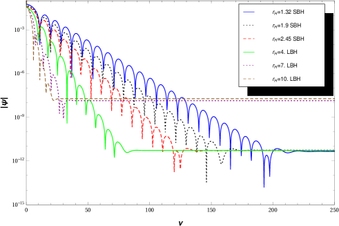
Figure 10: Time evolution of a scalar perturbation at the horizon of $\text{AdS}_{4}$ black holes (semi-log graph of $|\psi|$) for SBH with $r_{H}=1.32,1.9,2.45$ and LBH with $r_{H}=4,7,10$. The pressure is fixed at $P=P_{c}$

When the black hole (small and large) grows the damping rate increases and the perturbation decays faster while the oscillation time decreases, namely the oscillation frequencies increase. These features revealed via the time evolution analysis confirms the behavior of quasinormal frequencies in [1, 2].

5 Conclusion

In this paper, we studied the time evolution of a scalar perturbation around small and large $\text{RN-AdS}_{4}$ black holes for the purpose of probing the thermodynamic phase transition.

We found that below the critical point the scalar perturbation decays faster with increasing of the black hole size for both small and large black hole phase, but the oscillation frequencies become smaller and smaller with very slow variation.Unlike in time evolution, where the behavior analysis reveals that small and large black holes are in different phases, providing a tool to probe the BH phase transition.

At the critical point $P=P_{c}$, with growing sizes of the black hole, the damping time increases and the perturbation decays faster, the oscillation frequencies increase either in small and large black hole phase. In this case the time evolution of a scalar perturbation fails to detect the $\text{AdS}_{4}$ black hole phase transitions confirming the result of the frequency domain analysis.

At last, we would like to mention that it would be interesting to perform similar calculations either for higher-dimensional RN-AdS black holes or for other black holes configurations.

References

- [1] M. Chabab, H. El Moumni, S. Iraoui and K. Masmar, Behavior of quasinormal modes and high dimension RN–AdS black hole phase transition, Eur. Phys. J. C 76, no. 12, 676 (2016), arXiv:1606.08524.
- [2] Y. Liu, D. C. Zou and B. Wang, Signature of the Van der Waals like small-large charged AdS black hole phase transition in quasinormal modes, JHEP 1409 179, (2014), arXiv:1405.2644.
- [3] J. M. Maldacena, The Large N limit of superconformal field theories and supergravity, Int. J. Theor. Phys. 38, 1113 (1999) [Adv. Theor. Math. Phys. 2, 231 (1998)].
- [4] O. Aharony, S. S. Gubser, J. M. Maldacena, H. Ooguri and Y. Oz, Large N field theories, string theory and gravity, Phys. Rept. 323, 183 (2000).
- [5] S. A. Hartnoll, Lectures on holographic methods for condensed matter physics, Class. Quant. Grav. 26, 224002 (2009), arXiv:0903.3246.
- [6] N. Iqbal, H. Liu and M. Mezei, Lectures on holographic non-Fermi liquids and quantum phase transitions, arXiv:1110.3814.
- [7] R. G. Cai, S. He, L. Li and Y. L. Zhang, Holographic Entanglement Entropy in Insulator/Superconductor Transition, JHEP 1207, 088 (2012), arXiv:1203.6620.
- [8] J. Casalderrey-Solana, H. Liu, D. Mateos, K. Rajagopal and U. A. Wiedemann, Gauge/String Duality, Hot QCD and Heavy Ion Collisions, arXiv:1101.0618.
- [9] E. Witten, Anti-de Sitter space and holography, Adv. Theor. Math. Phys. 2, 253 (1998).
- [10] S. S. Gubser, I. R. Klebanov and A. M. Polyakov, Gauge theory correlators from noncritical string theory, Phys. Lett. B 428, 105 (1998).
- [11] H. El Moumni, Phase Transition of AdS Black Holes with Non Linear Source in the Holographic Framework, Int. J. Theo Phys Phys, doi:10.1007/s10773-016-3197-2, (2016).
- [12] D. Kubiznak and R. B. Mann, P-V criticality of charged AdS black holes, J. High Energy Phys. 1207, 033, (2012).
- [13] A. Belhaj, M. Chabab, H. El Moumni and M. B. Sedra, On Thermodynamics of AdS Black Holes in Arbitrary Dimensions, Chin. Phys. Lett. 29, 100401 (2012), arXiv:1210.4617.
- [14] A. Belhaj, M. Chabab, H. El. Moumni, L. Medari and M. B. Sedra, The Thermodynamical Behaviors of Kerr—Newman AdS Black Holes, Chin. Phys. Lett. 30, 090402 (2013), arXiv:1307.7421.
- [15] A. Belhaj, M. Chabab, H. El Moumni, K. Masmar and M. B. Sedra, Critical Behaviors of 3D Black Holes with a Scalar Hair, Int. J. Geom. Meth. Mod. Phys. 12, no. 02, 1550017 (2014), arXiv:1306.2518.
- [16] A. Belhaj, M. Chabab, H. El moumni, K. Masmar and M. B. Sedra, Maxwell‘s equal-area law for Gauss-Bonnet-Anti-de Sitter black holes, Eur. Phys. J. C 75, no. 2, 71 (2015), arXiv:1412.2162.
- [17] A. Belhaj, M. Chabab, H. El Moumni, K. Masmar, M. B. Sedra and A. Segui, On Heat Properties of AdS Black Holes in Higher Dimensions, JHEP 1505, 149 (2015), arXiv:1503.07308.
- [18] A. Belhaj, M. Chabab, H. El Moumni, K. Masmar and M. B. Sedra, On Thermodynamics of AdS Black Holes in M-Theory, Eur. Phys. J. C 76, no. 2, 73 (2016), arXiv:1509.02196.
- [19] M. Chabab, H. El Moumni and K. Masmar, On thermodynamics of charged AdS black holes in extended phases space via M2-branes background, Eur. Phys. J. C 76, no. 6, 304 (2016), arXiv:1512.07832.
- [20] S. Mahapatra, Thermodynamics, Phase Transition and Quasinormal modes with Weyl corrections, JHEP 1604, 142 (2016), arXiv:1602.03007.
- [21] B. P. Abbott et al. [LIGO Scientific and Virgo Collaborations], Observation of Gravitational Waves from a Binary Black Hole Merger, Phys. Rev. Lett. 116 061102 (2016), arXiv:1602.03837.
- [22] M. Armano et al., Sub-Femto- Free Fall for Space-Based Gravitational Wave Observatories: LISA Pathfinder Results, Phys. Rev. Lett. 116 no. 23, 231101 (2016).
- [23] A. Chamblin, R. Emparan, C. Johnson and R. Myers, Charged AdS black holes and catastrophic holography, Phys. Rev. D 60, 064018 (1999).
- [24] D. Kastor, S. Ray and J. Traschen, Enthalpy and the Mechanics of AdS Black Holes, Class. Quant. Grav. 261 95011 (2009), arXiv:0904.2765.
- [25] J. M. Zhu, B. Wang and E. Abdalla, Object picture of quasinormal ringing on the background of small Schwarzschild anti-de Sitter black holes, Phys. Rev. D 63 124004, (2001).
- [26] R. Li, H. Zhang and J. Zhao, Time evolutions of scalar field perturbations in D-dimensional Reissner–Nordström Anti-de Sitter black holes, Phys. Lett. B 758, 359 (2016), arXiv:1604.01267.
- [27] C. Gundlach, R. H. Price and J. Pullin, Late time behavior of stellar collapse and explosions: 1. Linearized perturbations, Phys. Rev. D 49, 883 (1994).
- [28] B. Wang, C. Y. Lin and C. Molina, Quasinormal behavior of massless scalar field perturbation in Reissner-Nordstrom anti-de Sitter spacetimes, Phys. Rev. D 70, 064025 (2004).
- [29] V. Santos, R. V. Maluf and C. A. S. Almeida, Quasinormal frequencies of self-dual black holes, Phys. Rev. D 93, no. 8, 084047 (2016), arXiv:1509.04306.
- [30] R. A. Konoplya and A. Zhidenko, Quasinormal modes of black holes: From astrophysics to string theory, Rev. Mod. Phys. 83 793 (2011), arXiv:1102.4014.
- [31] J. Morgan, V. Cardoso, A. S. Miranda, C. Molina and V. T. Zanchin, Quasinormal modes of black holes in anti-de Sitter space: A Numerical study of the eikonal limit, Phys. Rev. D 80 024024 (2009), arXiv:0906.0064.
- [32] X. He, B. Wang, R. G. Cai and C. Y. Lin, Signature of the black hole phase transition in quasinormal modes, Phys. Lett. B 688 230 (2010), arXiv:1002.2679.
- [33] T. R. Choudhury and T. Padmanabhan, Quasinormal modes in Schwarzschild-deSitter space-time: A Simple derivation of the level spacing of the frequencies, Phys. Rev. D 69, 064033 (2004).
- [34] Z. Zhu, S. J. Zhang, C. E. Pellicer, B. Wang and E. Abdalla, Stability of Reissner-Nordström black hole in de Sitter background under charged scalar perturbation, Phys. Rev. D 90, no. 4, 044042 (2014), arXiv:1405.4931.
- [35] B. Toshmatov, Z. Stuchlík, J. Schee and B. Ahmedov, Quasinormal frequencies of black hole in the braneworld, Phys. Rev. D 93, no. 12, 124017 (2016), arXiv:1605.02058.
- [36] B. Wang, C. Molina and E. Abdalla, Evolving of a massless scalar field in Reissner-Nordstrom Anti-de Sitter space-times, Phys. Rev. D 63, 084001 (2001).
- [37] C. B. M. H. Chirenti and L. Rezzolla, How to tell a gravastar from a black hole, Class. Quant. Grav. 24, 4191 (2007), arXiv:0706.1513.