Learning a Mixture of Deep Networks for Single Image Super-Resolution

Abstract

Single image super-resolution (SR) is an ill-posed problem which aims to recover high-resolution (HR) images from their low-resolution (LR) observations. The crux of this problem lies in learning the complex mapping between low-resolution patches and the corresponding high-resolution patches. Prior arts have used either a mixture of simple regression models or a single non-linear neural network for this propose. This paper proposes the method of learning a mixture of SR inference modules in a unified framework to tackle this problem. Specifically, a number of SR inference modules specialized in different image local patterns are first independently applied on the LR image to obtain various HR estimates, and the resultant HR estimates are adaptively aggregated to form the final HR image. By selecting neural networks as the SR inference module, the whole procedure can be incorporated into a unified network and be optimized jointly. Extensive experiments are conducted to investigate the relation between restoration performance and different network architectures. Compared with other current image SR approaches, our proposed method achieves state-of-the-arts restoration results on a wide range of images consistently while allowing more flexible design choices. The source codes are available in http://www.ifp.illinois.edu/~dingliu2/accv2016.

1 Introduction

Single image super-resolution (SR) is usually cast as an inverse problem of recovering the original high-resolution (HR) image from the low-resolution (LR) observation image. This technique can be utilized in the applications where high resolution is of importance, such as photo enhancement, satellite imaging and SDTV to HDTV conversion [1]. The main difficulty resides in the loss of much information in the degradation process. Since the known variables from the LR image is usually greatly outnumbered by that from the HR image, this problem is a highly ill-posed problem.

A large number of single image SR methods have been proposed in the literature, including interpolation based method [2], edge model based method [3] and example based method [4, 5, 6, 7, 8, 9]. Since the former two methods usually suffer the sharp drop in restoration performance with large upscaling factors, the example based method draws great attention from the community recently. It usually learns the mapping from LR images to HR images in a patch-by-patch manner, with the help of sparse representation [6, 10], random forest [11] and so on. The neighbor embedding method [4, 7] and neural network based method [8] are two representatives of this category.

Neighbor embedding is proposed in [4, 12] which estimates HR patches as a weighted average of local neighbors with the same weights as in LR feature space, based on the assumption that LR/HR patch pairs share similar local geometry in low-dimensional nonlinear manifolds. The coding coefficients are first acquired by representing each LR patch as a weighted average of local neighbors, and then the HR counterpart is estimated by the multiplication of the coding coefficients with the corresponding training HR patches. Anchored neighborhood regression (ANR) is utilized in [7] to improve the neighbor embedding methods, which partitions the feature space into a number of clusters using the learned dictionary atoms as a set of anchor points. A regressor is then learned for each cluster of patches. This approach has demonstrated superiority over the counterpart of global regression in [7]. Other variants of learning a mixture of SR regressors can be found in [13, 14, 15].

Recently, neural network based models have demonstrated the strong capability for single image SR [16, 8, 17], due to its large model capacity and the end-to-end learning strategy to get rid of hand-crafted features. Cui et al. [16] propose using a cascade of stacked collaborative local autoencoders for robust matching of self-similar patches, in order to increase the resolution of inputs gradually. Dong et al. [8] exploit a fully convolutional neural network (CNN) to approximate the complex non-linear mapping between the LR image and the HR counterpart. A neural network that closely mimics the sparse coding approach for image SR is designed by Wang et al [17, 18]. Kim et al proposes a very deep neural network with residual architecture to exploit contextual information over large image regions [19].

In this paper, we propose a method to combine the merits of the neighborhood embedding methods and the neural network based methods via learning a mixture of neural networks for single image SR. The entire image signal space can be partitioned into several subspaces, and we dedicate one SR module to the image signals in each subspace, the synergy of which allows a better capture of the complex relation between the LR image signal and its HR counterpart than the generic model. In order to take advantage of the end-to-end learning strategy of neural network based methods, we choose neural networks as the SR inference modules and incorporate these modules into one unified network, and design a branch in the network to predict the pixel-level weights for HR estimates from each SR module before they are adaptively aggregated to form the final HR image.

A systematic analysis of different network architectures is conducted with the focus on the relation between SR performance and various network architectures via extensive experiments, where the benefit of utilizing a mixture of SR models is demonstrated. Our proposed approach is contrasted with other current popular approaches on a large number of test images, and achieves state-of-the-arts performance consistently along with more flexibility of model design choices.

The paper is organized as follows. The proposed method is introduced and explained in detail in Section 2. Section 3 describes our experiments, in which we analyze thoroughly different network architectures and compare the performance of our method with other current SR methods both quantitatively and qualitatively. Finally in Section 4 we conclude the paper.

2 Proposed Method

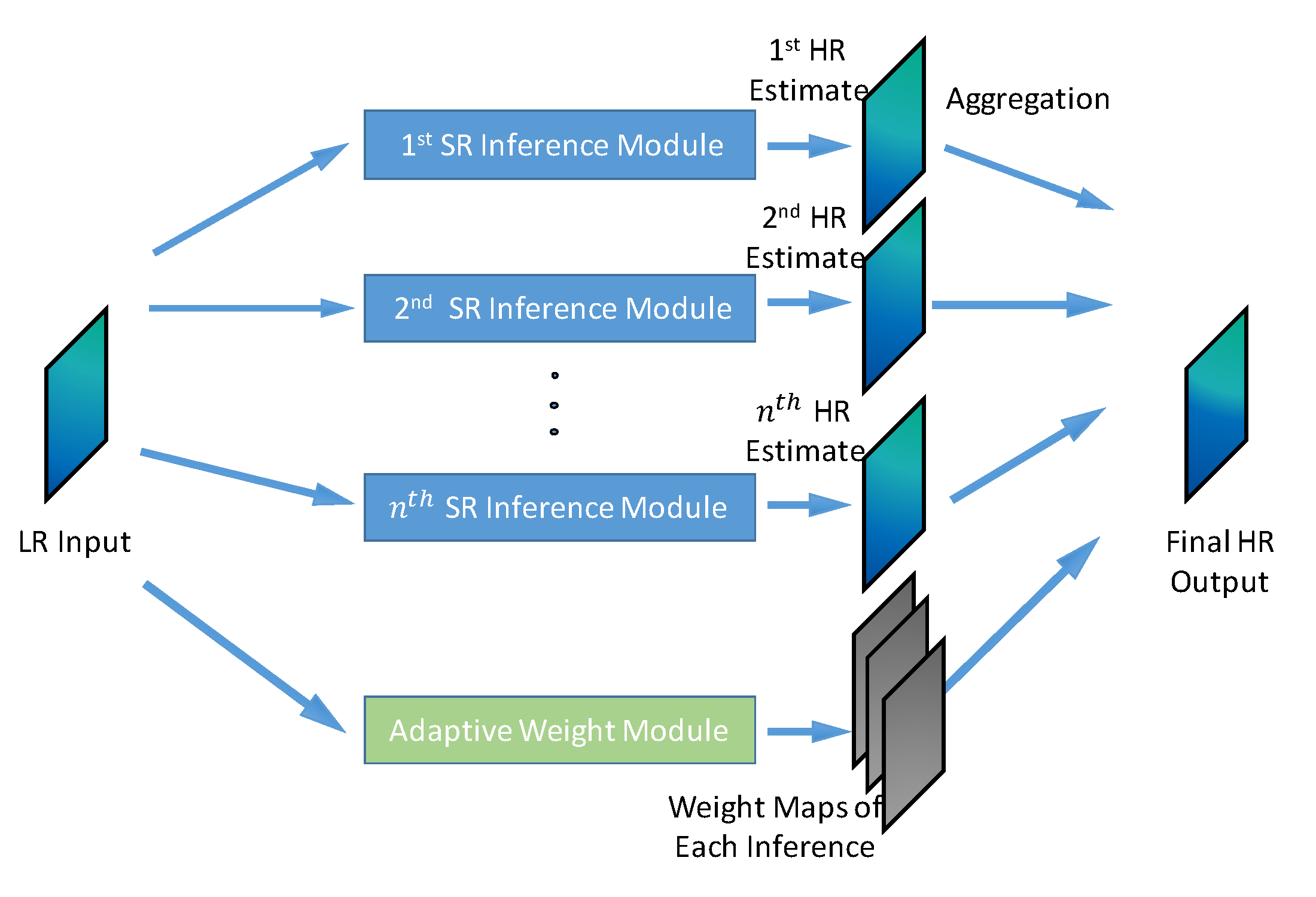
Figure 1: The overview of our proposed method. It consists of a number of SR inference modules and an adaptive weight module. Each SR inference module is dedicated to inferencing a certain class of image local patterns, and is independently applied on the LR image to predict one HR estimate. These estimates are adaptively combined using pixel-wise aggregation weights from the adaptive weight module in order to form the final HR image.

2.1 Overview

First we give the overview of our method. The LR image serves as the input to our method. There are a number of SR inference modules $\{B_{i}\}_{i=1}^{N}$ in our method. Each of them, $B_{i}$, is dedicated to inferencing a certain class of image patches, and applied on the LR input image to predict a HR estimate. We also devise an adaptive weight module, $T$, to adaptively combine at the pixel-level the HR estimates from SR inference modules. When we select neural networks as the SR inference modules, all the components can be incorporated into a unified neural network and be jointly learned. The final estimated HR image is adaptively aggregated from the estimates of all SR inference modules. The overview of our method is shown in Figure 1.

2.2 Network Architecture

2.2.1 SR Inference Module

: Taking the LR image as input, each SR inference module is designed to better capture the complex relation between a certain class of LR image signals and its HR counterpart, while predicting a HR estimate. For the sake of inference accuracy, we choose as the SR inference module a recent sparse coding based network (SCN) in [17], which implicitly incorporates the sparse prior into neural networks via employing the learned iterative shrinkage and thresholding algorithm (LISTA), and closely mimics the sparse coding based image SR method [20]. The architecture of SCN is shown in Figure 2. Note that the design of the SR inference module is not limited to SCN, and all other neural network based SR models, e.g. SRCNN [8], can work as the SR inference module as well. The output of $B_{i}$ serves as an estimate to the final HR frame.

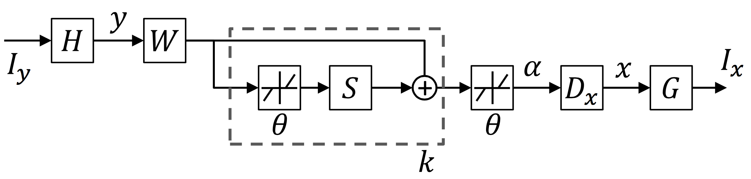
Figure 2: The network architecture of SCN [17], which serves as the SR inference module in our method.

2.2.2 Adaptive Weight Module

: The goal of this module is to model the selectivity of the HR estimates from every SR inference module. We propose assigning pixel-wise aggregation weights of each HR estimate, and again the design of this module is open to any operation in the field of neural networks. Taking into account the computation cost and efficiency, we utilize only three convolutional layers for this module, and ReLU is applied on the filter responses to introduce non-linearity. This module finally outputs the pixel-level weight maps for all the HR estimates.

2.2.3 Aggregation

: Each SR inference module’s output is pixel-wisely multiplied with its corresponding weight map from the adaptive weight module, and then these products are summed up to form the final estimated HR frame. If we use $\mathbf{y}$ to denote the LR input image, a function $W(\mathbf{y};\theta_{w})$ with parameters $\theta_{w}$ to represent the behavior of the adaptive weight module, and a function $F_{B_{i}}(\mathbf{y};\theta_{B_{i}})$ with parameters $\theta_{B_{i}}$ to represent the output of SR inference module $B_{i}$, the final estimated HR image $F(\mathbf{y};\mathbf{\Theta})$ can be expressed as

$$F(\mathbf{y};\mathbf{\Theta})=\sum_{i=1}^{N}W_{i}(\mathbf{y};\theta_{w})\odot F_{B_{i}}(\mathbf{y};\theta_{B_{i}}),$$ (1)

where $\odot$ denotes the point-wise multiplication.

2.3 Training Objective

In training, our model tries to minimize the loss between the target HR frame and the predicted output, as

$$％\vspace{-2mm}\min\limits_{\mathbf{\Theta}}\sum_{j}\|F(\mathbf{y}_{j};\mathbf{\Theta})-\mathbf{x}_{j}\|^{2}_{2},$$ (2)

where $F(\mathbf{y};\mathbf{\Theta})$ represents the output of our model, $\mathbf{x}_{j}$ is the $j$-th HR image and $\mathbf{y}_{j}$ is the corresponding LR image; $\mathbf{\Theta}$ is the set of all parameters in our model.

If we plug Eqn. 1 into Eqn. 2, the cost function then can be expanded as:

$$\min\limits_{\theta_{w},\{\theta_{B_{i}}\}_{i=1}^{N}}\sum_{j}\|\sum_{i=1}^{N}W_{i}(\mathbf{y}_{j};\theta_{w})\odot F_{B_{i}}(\mathbf{y}_{j};\theta_{B_{i}})-\mathbf{x}_{j}\|^{2}_{2}.$$ (3)

3 Experiments

3.1 Data Sets and Implementation Details

We conduct experiments following the protocols in [7]. Different learning based methods use different training data in the literature. We choose 91 images proposed in [6] to be consistent with [13, 11, 17]. These training data are augmented with translation, rotation and scaling, providing approximately 8 million training samples of $56\times 56$ pixels.

Our model is tested on three benchmark data sets, which are Set5 [12], Set14 [21] and BSD100 [22]. The ground truth images are downscaled by bicubic interpolation to generate LR/HR image pairs for both training and testing.

Following the convention in [7, 17], we convert each color image into the YCbCr colorspace and only process the luminance channel with our model, and bicubic interpolation is applied to the chrominance channels, because the visual system of human is more sensitive to details in intensity than in color.

Each SR inference module adopts the network architecture of SCN, while the filters of all three convolutional layers in the adaptive weight module have the spatial size of $5\times 5$ and the numbers of filters of three layers are set to be $32,16$ and $N$, which is the number of SR inference modules.

Our network is implemented using Caffe [23] and is trained on a machine with 12 Intel Xeon 2.67GHz CPUs and 1 Nvidia TITAN X GPU. For the adaptive weight module, we employ a constant learning rate of $10^{-5}$ and initialize the weights from Gaussian distribution, while we stick to the learning rate and the initialization method in [17] for the SR inference modules. The standard gradient descent algorithm is employed to train our network with a batch size of 64 and the momentum of 0.9.

We train our model for the upscaling factor of 2. For larger upscaling factors, we adopt the model cascade technique in [17] to apply $\times 2$ models multiple times until the resulting image reaches at least as large as the desired size. The resulting image is downsized via bicubic interpolation to the target resolution if necessary.

Table 1: PSNR (in dB) and SSIM comparisons on Set5, Set14 and BSD100 for $\times 2$, $\times 3$ and $\times 4$ upscaling factors among various network architectures. Red indicates the best and blue indicates the second best performance.

Benchmark		SCN	MSCN-2	MSCN-4
		($n=128$)	($n=64$)	($n=32$)
Set5	$\times 2$	36.93 / 0.9552	37.00 / 0.9558	36.99 / 0.9559
	$\times 3$	33.10 / 0.9136	33.15 / 0.9133	33.13 / 0.9130
	$\times 4$	30.86 / 0.8710	30.92 / 0.8709	30.93 / 0.8712
Set14	$\times 2$	32.56 / 0.9069	32.70 / 0.9074	32.72 / 0.9076
	$\times 3$	29.41 / 0.8235	29.53 / 0.8253	29.56 / 0.8256
	$\times 4$	27.64 / 0.7578	27.76 / 0.7601	27.79 / 0.7607
BSD100	$\times 2$	31.40 / 0.8884	31.54 / 0.8913	31.56 / 0.8914
	$\times 3$	28.50 / 0.7885	28.56 / 0.7920	28.59 / 0.7926
	$\times 4$	27.03 / 0.7161	27.10 / 0.7207	27.13 / 0.7216

3.2 SR Performance vs. Network Architecture

In this section we investigate the relation between various numbers of SR inference modules and SR performance. For the sake of our analysis, we increase the number of inference modules as we decrease the module capacity of each of them, so that the total model capacity is approximately consistent and thus the comparison is fair. Since the chosen SR inference module, SCN [17], closely mimics the sparse coding based SR method, we can reduce the module capacity of each inference module by decreasing the embedded dictionary size $n$ (i.e. the number of filters in SCN), for sparse representation. We compare the following cases:

• one inference module with $n=128$, which is equivalent to the structure of SCN in [17], denoted as SCN (n=128). Note that there is no need to include the adaptive weight module in this case.

• two inference modules with $n=64$, denoted as MSCN-2 (n=64).

• four inference modules with $n=32$, denoted as MSCN-4 (n=32).

The average Peak Signal-to-Noise Ratio (PSNR) and structural similarity (SSIM) [24] are measured to quantitatively compare the SR performance of these models over Set5, Set14 and BSD100 for various upscaling factors ($\times 2,\times 3,\times 4$), and the results are displayed in Table 1.

It can be observed that MSCN-2 (n=64) usually outperforms the original SCN network, i.e. SCN (n=128), and MSCN-4 (n=32) can achieve the best SR performance by improving the performance marginally over MSCN-2 (n=64). This demonstrates the effectiveness of our approach that each SR inference model is able to super-resolve its own class of image signals better than one single generic inference model.

Weight map 1
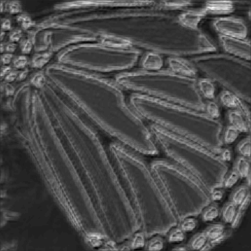
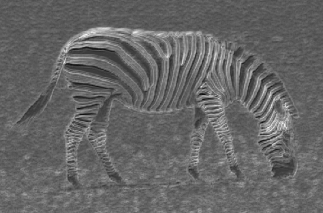
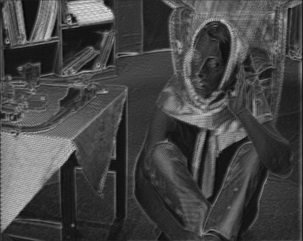
Weight map 2
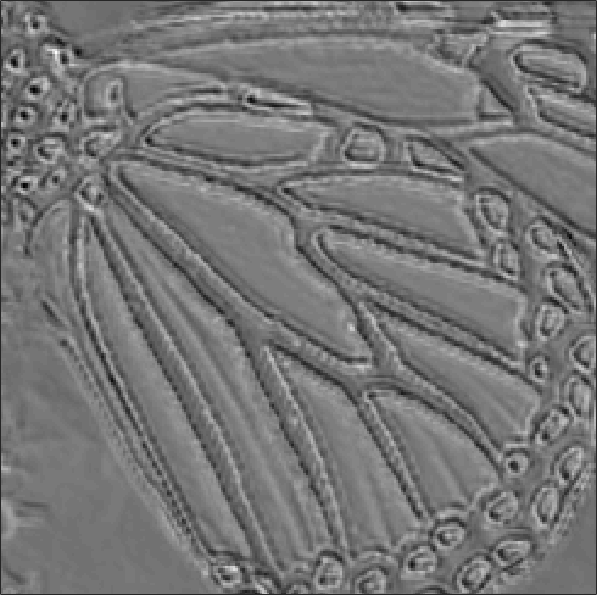
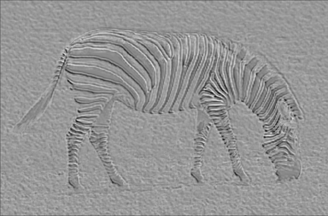
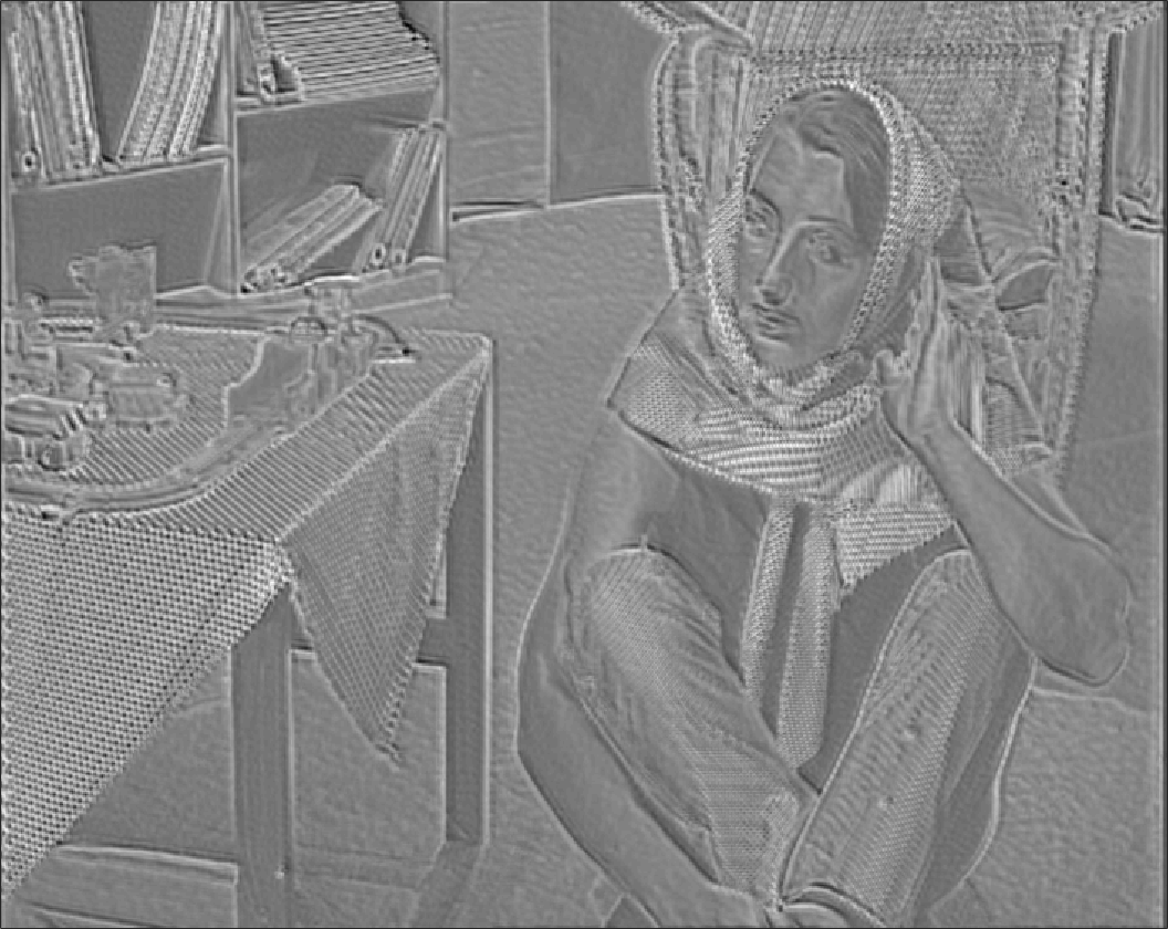
Weight map 3
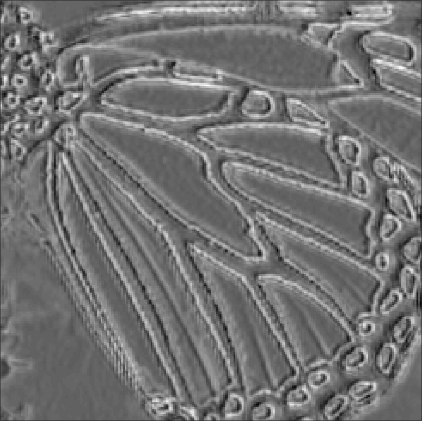
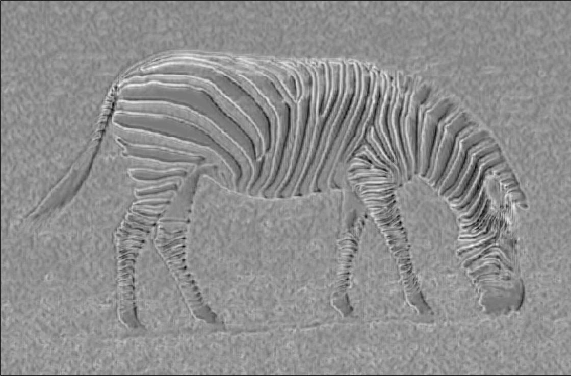
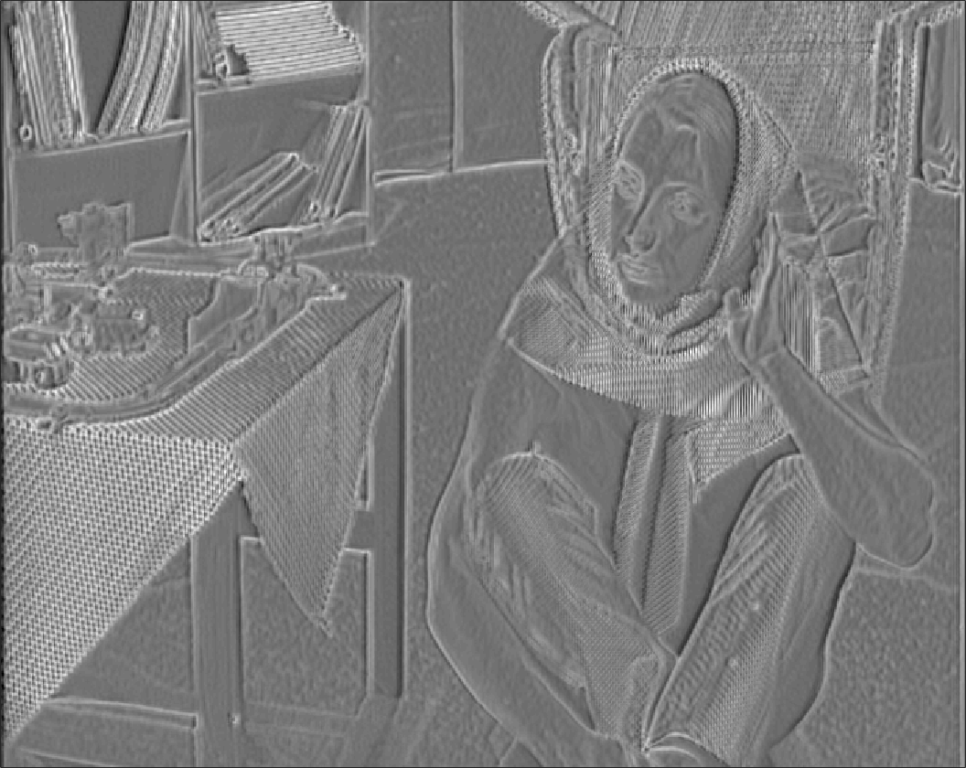
Weight map 4
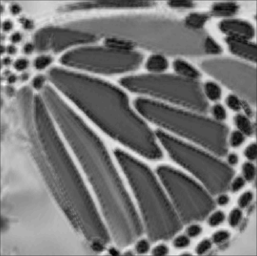
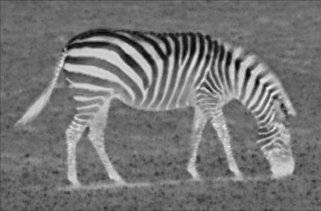
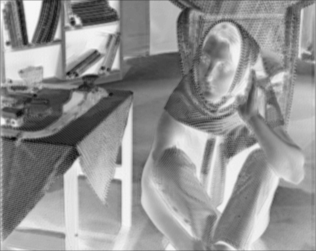
Max label map

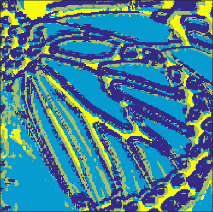
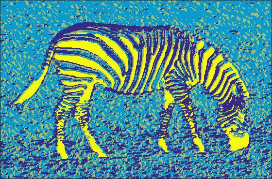
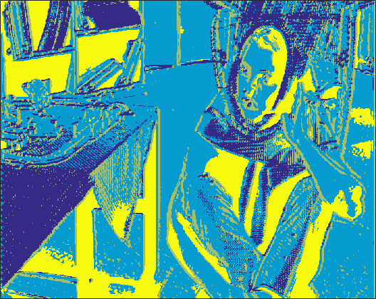
Figure 3: Weight maps for the HR estimate from every SR inference module in MSCN-4 are given in the first four rows. The map (max label map) which records the index of the maximum weight across all weight maps at every pixel is shown in the last row. Images from left to right: the butterfly image upscaled by $\times 2$; the zebra image upscaled by $\times 2$; the barbara image upscaled by $\times 2$.

In order to further analyze the adaptive weight module, we select several input images, namely, butterfly, zebra, barbara, and visualize the four weight maps for every SR inference module in the network. Moreover, we record the index of the maximum weight across all weight maps at every pixel and generate a max label map. These results are displayed in Figure 3.

From these visualizations it can be seen that weight map 4 shows high responses in many uniform regions, and thus mainly contributes to the low frequency regions of HR predictions. On the contrary, weight map 1, 2 and 3 have large responses in regions with various edges and textures, and restore the high frequency details of HR predictions. These weight maps reveal that these sub-networks work in a supplementary manner for constructing the final HR predictions. In the max label map, similar structures and patterns of images usually share with the same label, indicating that such similar textures and patterns are favored to be super-resolved by the same inference model.

Table 2: PSNR (SSIM) comparison on three test data sets for various upscaling factors among different methods. The best performance is indicated in red and the second best performance is shown in blue. The performance gain of our best model over all the other models’ best is shown in the last row.

Data Set	Set5			Set14			BSD100
Upscaling	$\times 2$	$\times 3$	$\times 4$	$\times 2$	$\times 3$	$\times 4$	$\times 2$	$\times 3$	$\times 4$
A+ [13]	36.55	32.59	30.29	32.28	29.13	27.33	31.21	28.29	26.82
	(0.9544)	(0.9088)	(0.8603)	(0.9056)	(0.8188)	(0.7491)	(0.8863)	(0.7835)	(0.7087)
SRCNN [8]	36.66	32.75	30.49	32.45	29.30	27.50	31.36	28.41	26.90
	(0.9542)	(0.9090)	(0.8628)	(0.9067)	(0.8215)	(0.7513)	(0.8879)	(0.7863)	(0.7103)
RFL [11]	36.54	32.43	30.14	32.26	29.05	27.24	31.16	28.22	26.75
	(0.9537)	(0.9057)	(0.8548)	(0.9040)	(0.8164)	(0.7451)	(0.8840)	(0.7806)	(0.7054)
SelfEx [9]	36.49	32.58	30.31	32.22	29.16	27.40	31.18	28.29	26.84
	(0.9537)	(0.9093)	(0.8619)	(0.9034)	(0.8196)	(0.7518)	(0.8855)	(0.7840)	(0.7106)
SCN [17]	36.93	33.10	30.86	32.56	29.41	27.64	31.40	28.50	27.03
	(0.9552)	(0.9144)	(0.8732)	(0.9074)	(0.8238)	(0.7578)	(0.8884)	(0.7885)	(0.7161)
MSCN-4	37.16	33.33	31.08	32.85	29.65	27.87	31.65	28.66	27.19
	(0.9565)	(0.9155)	(0.8740)	(0.9084)	(0.8272)	(0.7624)	(0.8928)	(0.7941)	(0.7229)
Our	0.23	0.23	0.22	0.29	0.24	0.23	0.25	0.16	0.16
Improvement	(0.0013)	(0.0011)	(0.0008)	(0.0010)	(0.0034)	(0.0046)	(0.0044)	(0.0056)	(0.0068)

A+ [13]
SRCNN [8]
SCN [17]
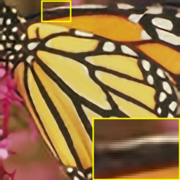
MSCN-4
Ground Truth
	(a) ppt3	(b) 102061	(c) butterfly

Figure 4: Visual comparisons of SR results among different methods. From left to right: the ppt3 image upscaled by $\times 3$; the 102061 image upscaled by $\times 3$; the butterfly image upscaled by $\times 4$.

3.3 Comparison with State-of-the-Arts

We conduct experiments on all the images in Set5, Set14 and BSD100 for different upscaling factors ($\times 2,\times 3,$ and $\times 4$), to quantitatively and qualitatively compare our own approach with a number of state-of-the-arts image SR methods. Table 2 shows the PSNR and SSIM for adjusted anchored neighborhood regression (A+) [13], SRCNN [8], RFL [11], SelfEx [9] and our proposed model, MSCN-4 (n=128) , that consists of four SCN modules with $n=128$. The single generic SCN without multi-view testing in [17], i.e. SCN (n=128) is also included for comparison as the baseline. Note that all the methods use the same 91 images [6] for training except SRCNN [8], which uses 395,909 images from ImageNet as training data.

It can be observed that our proposed model achieves the best SR performance consistently over three data sets for various upscaling factors. It outperforms SCN (n=128) which obtains the second best results by about 0.2dB across all the data sets, owing to the power of multiple inference modules.

We compare the visual quality of SR results among various methods in Figure 4. The region inside the bounding box is zoomed in and shown for the sake of visual comparison. Our proposed model MSCN-4 (n=128) is able to recover sharper edges and generate less artifacts in the SR inferences.

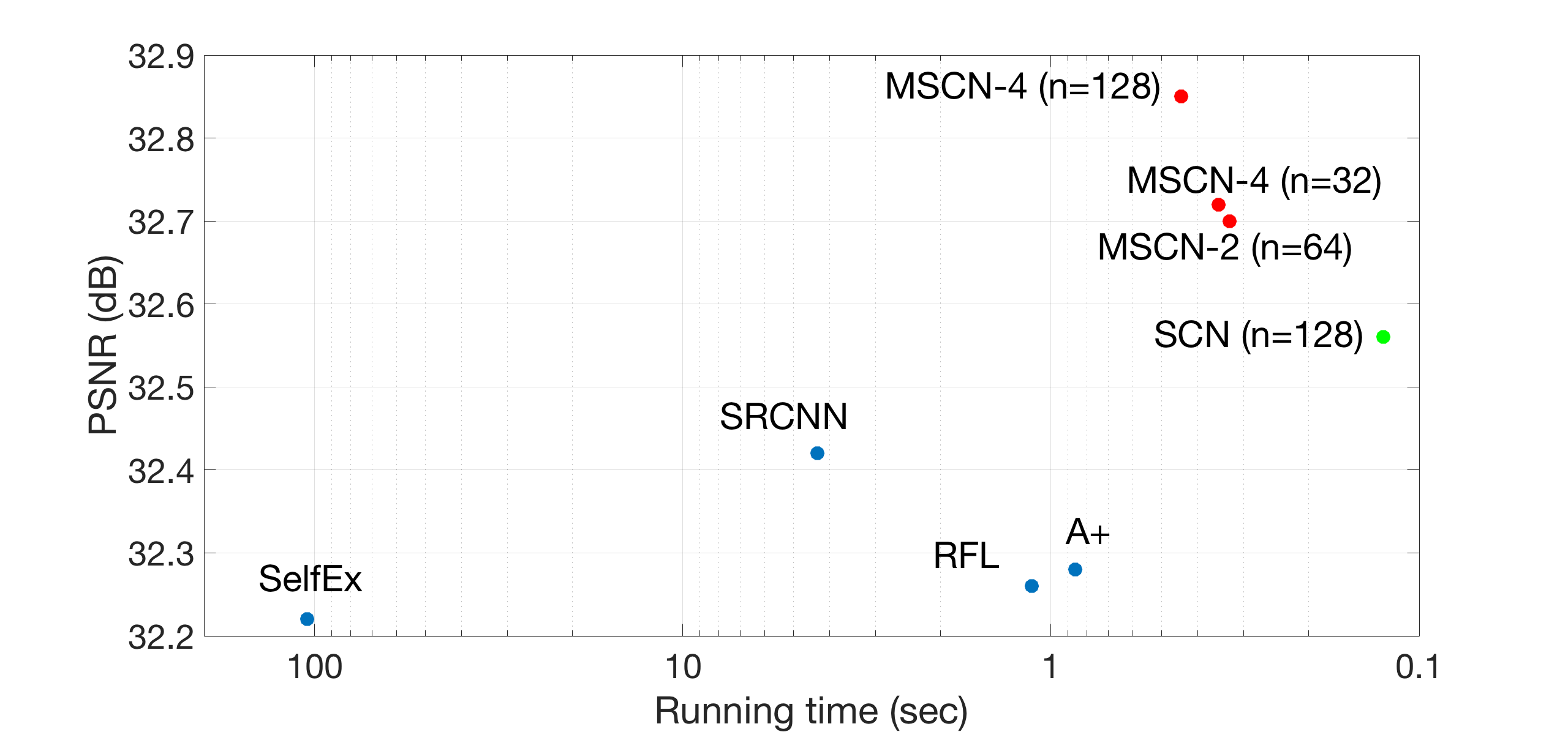
Figure 5: The average PSNR and the average inference time for upscaling factor $\times 2$ on Set14 are compared among different network structures of our method and other SR methods. SRCNN uses the public slower implementation of CPU.

3.4 SR Performance vs. Inference Time

The inference time is an important factor of SR algorithms other than the SR performance. The relation between the SR performance and the inference time of our approach is analyzed in this section. Specifically, we measure the average inference time of different network structures in our method for upscaling factor $\times 2$ on Set14. The inference time costs versus the PSNR values are displayed in Figure 5, where several other current SR methods [9, 11, 8, 13] are included as reference (the inference time of SRCNN is from the public slower implementation of CPU). We can see that generally, the more modules our network has, the more inference time is needed and the better SR results are achieved. By adjusting the number of SR inference modules in our network structure, we can achieve the tradeoff between SR performance and computation complexity. However, our slowest network still has the superiority in term of inference time, compared with other previous SR methods.

4 Conclusions

In this paper, we propose to jointly learn a mixture of deep networks for single image super-resolution, each of which serves as a SR inference module to handle a certain class of image signals. An adaptive weight module is designed to predict pixel-level aggregation weights of the HR estimates. Various network architectures are analyzed in terms of the SR performance and the inference time, which validates the effectiveness of our proposed model design. Extensive experiments manifest that our proposed model is able to achieve outstanding SR performance along with more flexibility of design. In the future, this approach of image super-resolution will be explored to facilitate other high-level vision tasks [25].

References

- [1] Park, S.C., Park, M.K., Kang, M.G.: Super-resolution image reconstruction: a technical overview. Signal Processing Magazine, IEEE 20 (2003) 21–36
- [2] Morse, B.S., Schwartzwald, D.: Image magnification using level-set reconstruction. In: CVPR 2001. Volume 1., IEEE (2001) I–333
- [3] Fattal, R.: Image upsampling via imposed edge statistics. In: ACM Transactions on Graphics (TOG). Volume 26., ACM (2007) 95
- [4] Chang, H., Yeung, D.Y., Xiong, Y.: Super-resolution through neighbor embedding. In: Computer Vision and Pattern Recognition, 2004. CVPR 2004. Proceedings of the 2004 IEEE Computer Society Conference on. Volume 1., IEEE (2004) I–I
- [5] Glasner, D., Bagon, S., Irani, M.: Super-resolution from a single image. In: ICCV 2009, IEEE (2009) 349–356
- [6] Yang, J., Wright, J., Huang, T.S., Ma, Y.: Image super-resolution via sparse representation. IEEE Transactions on Image Processing 19 (2010) 2861–2873
- [7] Timofte, R., De, V., Van Gool, L.: Anchored neighborhood regression for fast example-based super-resolution. In: Computer Vision (ICCV), 2013 IEEE International Conference on, IEEE (2013) 1920–1927
- [8] Dong, C., Loy, C.C., He, K., Tang, X.: Image super-resolution using deep convolutional networks. TPAMI (2015)
- [9] Huang, J.B., Singh, A., Ahuja, N.: Single image super-resolution from transformed self-exemplars. In: Computer Vision and Pattern Recognition (CVPR), 2015 IEEE Conference on, IEEE (2015) 5197–5206
- [10] Wang, Z., Yang, Y., Wang, Z., Chang, S., Yang, J., Huang, T.S.: Learning super-resolution jointly from external and internal examples. IEEE Transactions on Image Processing 24 (2015) 4359–4371
- [11] Schulter, S., Leistner, C., Bischof, H.: Fast and accurate image upscaling with super-resolution forests. In: Proceedings of the IEEE Conference on Computer Vision and Pattern Recognition. (2015) 3791–3799
- [12] Bevilacqua, M., Roumy, A., Guillemot, C., Alberi-Morel, M.L.: Low-complexity single-image super-resolution based on nonnegative neighbor embedding. (2012)
- [13] Timofte, R., De Smet, V., Van Gool, L.: A+: Adjusted anchored neighborhood regression for fast super-resolution. In: Computer Vision–ACCV 2014. Springer (2014) 111–126
- [14] Dai, D., Timofte, R., Van Gool, L.: Jointly optimized regressors for image super-resolution. In: Eurographics. Volume 7. (2015) 8
- [15] Timofte, R., Rasmus, R., Van Gool, L.: Seven ways to improve example-based single image super resolution. In: Computer Vision and Pattern Recognition (CVPR), 2016 IEEE Conference on, IEEE (2016)
- [16] Cui, Z., Chang, H., Shan, S., Zhong, B., Chen, X.: Deep network cascade for image super-resolution. In: Computer Vision–ECCV 2014. Springer (2014) 49–64
- [17] Wang, Z., Liu, D., Yang, J., Han, W., Huang, T.: Deep networks for image super-resolution with sparse prior. In: Proceedings of the IEEE International Conference on Computer Vision. (2015) 370–378
- [18] Liu, D., Wang, Z., Wen, B., Yang, J., Han, W., Huang, T.S.: Robust single image super-resolution via deep networks with sparse prior. IEEE Transactions on Image Processing 25 (2016) 3194–3207
- [19] Kim, J., Lee, J.K., Lee, K.M.: Accurate image super-resolution using very deep convolutional networks. In: Computer Vision and Pattern Recognition (CVPR), 2016 IEEE Conference on, IEEE (2016)
- [20] Yang, J., Wang, Z., Lin, Z., Cohen, S., Huang, T.: Coupled dictionary training for image super-resolution. Image Processing, IEEE Transactions on 21 (2012) 3467–3478
- [21] Zeyde, R., Elad, M., Protter, M.: On single image scale-up using sparse-representations. In: Curves and Surfaces. Springer (2012) 711–730
- [22] Martin, D., Fowlkes, C., Tal, D., Malik, J.: A database of human segmented natural images and its application to evaluating segmentation algorithms and measuring ecological statistics. In: Computer Vision, 2001. ICCV 2001. Proceedings. Eighth IEEE International Conference on. Volume 2., IEEE (2001) 416–423
- [23] Jia, Y., Shelhamer, E., Donahue, J., Karayev, S., Long, J., Girshick, R., Guadarrama, S., Darrell, T.: Caffe: Convolutional architecture for fast feature embedding. In: Proceedings of the ACM International Conference on Multimedia, ACM (2014) 675–678
- [24] Wang, Z., Bovik, A.C., Sheikh, H.R., Simoncelli, E.P.: Image quality assessment: from error visibility to structural similarity. Image Processing, IEEE Transactions on 13 (2004) 600–612
- [25] Wang, Z., Chang, S., Yang, Y., Liu, D., Huang, T.: Studying very low resolution recognition using deep networks. In: Computer Vision and Pattern Recognition (CVPR), 2016 IEEE Conference on, IEEE (2016)