Resonant state expansion for Transverse Electric modes of two-dimensional open optical systems

Abstract

The resonant state expansion (RSE), a rigorous perturbative method in electrodynamics, is formulated for Transverse Electrodynamic modes of an effectively $2$-dimensional system. The RSE is a perturbation theory based on the Lippmann Schwinger Green’s function equation and requires knowledge of the Green’s function of the unperturbed system constructed from Resonant-states. I use the analytic Green’s function for the magnetic field to normalize the modes appearing in the corresponding spectral Green’s function. This use of the residue and cut of the analytic Green’s function is a solution to the failure of the flux volume integral method of normalization for continuum states, a problem which is discussed in detail in this manuscript. In brief, the flux volume integral fails for continuum states because they are not true resonance. An analytic relation between normalized magnetic and electric modes is developed as part of the solution to these difficulties. The complex eigenfrequencies of modes are calculated using the RSE for the case of a homogeneous perturbation.

I Introduction

Dielectric microcavities have attracted significant interest since 1989 when they were found to support whispering gallery modes (WGMs) Braginsky89 , particularly with regards to the development of hybrid optoelectronic circuits Vahala03 . Perturbed microcavities have proved to be the most promising direction of research since their emissions are not isotropic Nockel97 ; Gmachl98 ; Lee02 ; Harayama03 ; Chern03 ; Kurdoglyan04 ; Wiersig08 . Other uses of $2$-dimensional optical microcavities include miniature lasing devices Vahala44 .

Recently there has been developed the Resonant-state-expansion (RSE) a theory for calculating the resonances of open optical systems ArmitagePRA14 ; DoostPRA13 ; DoostPRA14 ; DoostPRA12 ; MuljarovEPL10 ; Doost_Muljarov . That the RSE is suitable for use with the RSE Born approximation, to calculate the far field scattering, has been demonstrated in Ref.Doost15 ; Doost16 ; Ge14 . The RSE Born approximation is a rigorous perturbation method for electrodynamic scattering, which becomes the exact solution of Maxwell’s wave equations in the far field, in the limit of an infinite number of resonance being taken into account in the Born approximation expansion.

In this paper I report extending the RSE to the Transverse Electric (TE) modes of effectively two-dimensional (2D) systems (i.e. 3D systems translational invariant in one dimension) which are not reducible to effective 1D systems. I only treat systems with zero wavevector along the translational invariant direction at present. I use a dielectric cylinder with uniform dielectric constant in vacuum as unperturbed system and calculate perturbed Resonant-states (RSs) for homogeneous perturbations in order to demonstrate the method.

The treatment in this manuscript is restricted to $2$-dimensional systems, however for the modes of a cavity with mode wavelength only a small fraction of the thickness of the cavity it is possible to make the mathematical approximation to an effectively $2$-dimensional system Smotrova05 ; Lebental07 . A consequence of this approximation for the mathematical treatment is that the refractive index $n_{r}$ has to be replace with an appropriately calculated $n_{eff}$ which takes into account the thickness of the resonator, for the detailed mathematics, see Ref.Smotrova05 ; Lebental07 .

In this manuscript dispersion in the refractive index is not treated directly, however it is straight-forward to add dispersion using the method from Ref.Doost_Muljarov , which I developed in collaboration with E. A. Muljarov, based on my successful initial independent work incorporating dispersion into the RSE.

Interestingly the RSE is a near identical translation to electrodynamics of a much earlier theory from Quantum Mechanics by More, Gerjuoy, Bang, Gareev, Gizzatkulov and Goncharov Ref.More73 ; Bang78 . The only difference between the two approaches is the choice of RS normalisation method. The RSE More73 ; Bang78 is a perturbation theory based on the Lippmann Schwinger Green’s function equation and requires knowledge of the Green’s function (GF) of the unperturbed system constructed from RSs. I was able to show in Ref.Doost15 that the general normalisation of RSs which I derived in Ref.DoostPRA14 is the most numerically stable available normalisation method. The general normalisation which I derived in Ref.DoostPRA14 is based on a prototype normalisation which appeared in Ref.MuljarovEPL10 .

One difficulty in formulating an RSE for 2D systems, is the presence of a one-dimensional continuum in the manifold of RSs. This continuum is specific to 2D systems and is required for the completeness of the basis and thus for the accuracy of the RSE applied in 2D, as discussed when similar observations were previously made for Transverse Magnetic (TM) modes of a microcylinder in my Ref.DoostPRA13 .

In Ref.DoostPRA13 ; DoostPRA14 it was shown that the continuum states in the RSE cannot be normalised by the flux volume normalisation,

$$1+\delta_{k_{n},0} = \int_{A}\mathbf{E}_{n}(\mathbf{\dot{r}})\cdot\dfrac{\partial\omega^{2}\hat{\boldsymbol{\varepsilon}}(\mathbf{\dot{r}},\omega)}{\partial\omega^{2}}\bigg{|}_{\omega=\omega_{n}}\!\!\mathbf{E}_{n}(\mathbf{\dot{r}})d{\mathbf{\dot{r}}}$$

$$+\lim_{k\rightarrow k_{n}}\oint_{L_{A}}\dfrac{\mathbf{E}_{n}\cdot\nabla\bf\mathbf{E}-\bf\mathbf{E}\cdot\nabla\mathbf{E}_{n}}{k^{2}-k^{2}_{n}}d{\bf L}$$

I will discuss the reason for this in more detail in Sec. III. Instead of using Eq. (I), it is necessary to make a comparison of the residue and contour integral between the spectral GF

$$\hat{\mathbf{G}}_{k}(\mathbf{r},\mathbf{r}^{\prime})=\hbox to0.0pt{$\displaystyle\sum_{n}$\hss}\int\,\frac{\mathbf{E}_{n}(\mathbf{r})\otimes\mathbf{E}_{n}(\mathbf{r}^{\prime})}{2k(k-k_{n})}\approx\sum_{\bar{n}}\frac{\phi_{\bar{n}}\mathbf{E}_{\bar{n}}(\mathbf{r})\otimes\mathbf{E}_{\bar{n}}(\mathbf{r}^{\prime})}{2k(k-k_{\bar{n}})}$$ (2)

and the analytically derived GF. The electrodynamic wave function $\mathbf{E}_{\bar{n}}$ is the solution to

$$\nabla\times\nabla\times\mathbf{E}_{\bar{n}}(\mathbf{r})=k^{2}_{\bar{n}}\hat{\boldsymbol{\varepsilon}}(\mathbf{r})\mathbf{E}_{\bar{n}}(\mathbf{r})$$ (3)

with outgoing boundary conditions (BCs) and $\hat{\mathbf{G}}_{k}(\mathbf{r},\mathbf{r}^{\prime})$ is the corresponding GF for Eq. (3).

Unfortunately it is not possible to derive the analytic GF for the electric $\bf\mathbf{E}$-field since for $2$-dimensional TE modes of an open system Maxwell’s wave equation is not reducible to one dimension whilst in the electric field description. However the magnetic $\bf\mathbf{H}$-field GF is available and in Appendix A I use physical arguments to construct an analytic formula linking normalised magnetic modes $\mathbf{H}_{\bar{n}}$ to normalised electric modes $\mathbf{E}_{\bar{n}}$. The analytic Green’s function for the homogeneous $2$-dimensional microcylinder is given in Appendix B.

This manuscript is organised as follows Sec. II outlines the derivation of the RSE perturbation theory, Sec. III explains the special provisions made for the normalisation of the $\mathbf{E}_{\bar{n}}$ modes, Sec. IV gives the basis modes of the $2$-dimensional RSE, Sec. V contains the numerical validation of the rigorous analytics provided in this manuscript, Appendix A and B derive the normalisation of the TE $\mathbf{E}_{\bar{n}}$ modes, Appendix C gives perturbation matrix elements required to reproduce the numerical results of Sec. V. Appendix D gives the evaluation of an important expression in Appendix A. Appendix E gives a new and valuable numerical recipe used in the production of numerical results for this manuscript.

II The RSE Perturbation method

In this section I give a brief account of the derivation of the RSE More73 ; Bang78 . The method of derivation is built upon the Lippmann Schwinger Green’s function equation. For a more detailed account of these derivations I direct the interested reader to Ref.More73 ; Bang78 ; ArmitagePRA14 ; DoostPRA13 ; DoostPRA14 ; DoostPRA12 ; MuljarovEPL10 ; Doost_Muljarov ; Doost15 ; Doost16 ; Ge14 .

The spectral representation of the 2D system GF is modified to include this cut contribution as integral DoostPRA13

$$\hat{\mathbf{G}}_{k}(\mathbf{r},\mathbf{r}^{\prime})=\hbox to0.0pt{$\displaystyle\sum_{n}$\hss}\int\,\frac{\mathbf{E}_{n}(\mathbf{r})\otimes\mathbf{E}_{n}(\mathbf{r}^{\prime})}{2k(k-k_{n})}\approx\sum_{\bar{n}}\frac{\phi_{\bar{n}}\mathbf{E}_{\bar{n}}(\mathbf{r})\otimes\mathbf{E}_{\bar{n}}(\mathbf{r}^{\prime})}{2k(k-k_{\bar{n}})}$$ (4)

In practice, the continuum of non-resonant states are discretised and included as cut poles in the perturbation basis. This problem is treated in depth in Appendix A, B and C. The combined index ${\bar{n}}$ is used to denote both real poles $k_{n}$ and cut poles $k_{\alpha}$ simultaneously. The weighting factors $\phi_{\bar{n}}$ are defined as follows

$$\phi_{\bar{n}}=\left\{\begin{array}[]{ll}\phi_{n}=1&{\rm for\ real\ poles},\\ \phi_{\alpha}&{\rm for\ cut\ poles}\\ \end{array}\right.$$ (5)

After modifying the expansion of the perturbed wave functions to include the cut poles to,

$$\mbox{\boldmath${\cal E}$}_{\nu}(\mathbf{r})=\sum_{\bar{n}}\phi_{\bar{n}}b_{\bar{n}\nu}\mathbf{E}_{\bar{n}}(\mathbf{r})$$ (6)

which is the solution to the equation,

$$\nabla\times\nabla\times\mbox{\boldmath${\cal E}$}_{\nu}(\mathbf{r})=\varkappa^{2}_{\nu}\left[\hat{\boldsymbol{\varepsilon}}(\mathbf{r})+\Delta\hat{\boldsymbol{\varepsilon}}(\mathbf{r})\right]\mbox{\boldmath${\cal E}$}_{\nu}(\mathbf{r})$$ (7)

with outgoing BCs, I can repeat the derivation of Ref.DoostPRA13 and make use of the Lippmann Schwinger Green’s function equation

$$\mbox{\boldmath${\cal E}$}_{\nu}(\mathbf{r})=-\varkappa^{2}_{\nu}\int\hat{\mathbf{G}}_{k}(\mathbf{r},\mathbf{r}^{\prime})\Delta\hat{\boldsymbol{\varepsilon}}(\mathbf{r}^{\prime})\mbox{\boldmath${\cal E}$}_{\nu}(\mathbf{r}^{\prime})d{\bf\mathbf{r}}^{\prime}$$ (8)

in conjuncture with the spectral GF

$$\hat{\mathbf{G}}_{k}(\mathbf{r},\mathbf{r}^{\prime})=\hbox to0.0pt{$\displaystyle\sum_{n}$\hss}\int\,\frac{\mathbf{E}_{n}(\mathbf{r})\otimes\mathbf{E}_{n}(\mathbf{r}^{\prime})}{2k(k-k_{n})}\approx\sum_{\bar{n}}\frac{\phi_{\bar{n}}\mathbf{E}_{\bar{n}}(\mathbf{r})\otimes\mathbf{E}_{\bar{n}}(\mathbf{r}^{\prime})}{2k(k-k_{\bar{n}})}$$ (9)

to arrive at the modified the RSE Matrix equations,

$$\varkappa_{\nu}\sum_{\bar{n}^{\prime}}\left(\delta_{\bar{n}\bar{n}^{\prime}}+\sqrt{\phi_{\bar{n}}\phi_{\bar{n}}^{\prime}}V_{\bar{n}{\bar{n}^{\prime}}}/2\right)b_{\bar{n}^{\prime}\nu}=k_{n}b_{\bar{n}\nu}$$ (10)

and

$$\sum_{\bar{n}^{\prime}}\left(\frac{\delta_{\bar{n}{\bar{n}}^{\prime}}}{k_{\bar{n}^{\prime}}}+\frac{V_{\bar{n}{\bar{n}}^{\prime}}}{2}\sqrt{\dfrac{\phi_{\bar{n}}\phi_{\bar{n}}^{\prime}}{k_{\bar{n}}k_{\bar{n}^{\prime}}}}\right)c_{{\bar{n}^{\prime}}\nu}=\frac{1}{\varkappa_{\nu}}c_{{\bar{n}}\nu}$$ (11)

As always $V_{\bar{n}\bar{n}^{\prime}}$ is given by

$$V_{\bar{n}\bar{n}^{\prime}}=\int\mathbf{E}_{\bar{n}}(\mathbf{r})\Delta\hat{\boldsymbol{\varepsilon}}(\mathbf{r})\mathbf{E}_{\bar{n}^{\prime}}(\mathbf{r})\,d\mathbf{r}$$ (12)

The perturbation method which I have briefly outlined was recently translated from Quantum Mechanics More73 ; Bang78 and has now become known as the Resonant-state-expansion.

III Maxwell’s wave equation for magnetic field

In this section I discuss the numerical and analytic difficulties associated with constructing an electrodynamic RSE perturbation theory for magnetic resonances.

If we examine Maxwell’s wave equation for magnetic field $\mathbf{H(\mathbf{r})}$,

$$-\nabla\times\nabla\times\mathbf{H(\mathbf{r})}+{\hat{\boldsymbol{\varepsilon}}({\bf r})}^{-1}{\nabla\hat{\boldsymbol{\varepsilon}}({\bf r})}\times(\nabla\times\mathbf{H(\mathbf{r})})+k^{2}\hat{\boldsymbol{\varepsilon}}({\bf r})\mathbf{H(\mathbf{r})}\\ =\nabla\times\mathbf{J(\mathbf{r})}-{\hat{\boldsymbol{\varepsilon}}({\bf r})}^{-1}{\nabla\hat{\boldsymbol{\varepsilon}}({\bf r})}\times\mathbf{J(\mathbf{r})}$$ (13)

it would at first sight seem of no use to the RSE. In Eq. (13) we can see $\nabla\hat{\boldsymbol{\varepsilon}}({\bf r})$ which has prevented me from formulating an equation analogous to Eq. (8) relating the perturbed eigenmodes of magnetic field to their unperturbed GF and perturbation in the dielectric profile. Therefore as I am considering perturbations in the dielectric profile I am forced to formulate the RSE in terms of electric modes $\mathbf{E}_{\bar{n}}(\mathbf{r})$.

However even in light of the previous paragraph I do need to consider Eq. (13) in this paper because the cut poles cannot be normalised using DoostPRA14 ; Doost16

$$1+\delta_{k_{n},0} = \int_{A}\mathbf{E}_{n}(\mathbf{\dot{r}})\cdot\dfrac{\partial\omega^{2}\hat{\boldsymbol{\varepsilon}}(\mathbf{\dot{r}},\omega)}{\partial\omega^{2}}\bigg{|}_{\omega=\omega_{n}}\!\!\mathbf{E}_{n}(\mathbf{\dot{r}})d{\mathbf{\dot{r}}}$$

$$+\lim_{k\rightarrow k_{n}}\oint_{L_{A}}\dfrac{\mathbf{E}_{n}\cdot\nabla\bf\mathbf{E}-\bf\mathbf{E}\cdot\nabla\mathbf{E}_{n}}{k^{2}-k^{2}_{n}}d{\bf L}$$

The method of normalisation will thus make use of Eq. (13). The reason I can’t use Eq. (III) for the cut poles is that they are not true resonances of the system. This problem can be intuitively understood if we assume we can normalise a single cut pole with Eq. (III) and observe the resulting logical contradiction. If the discretisation of the cut is made finer by increasing the number of cut poles by several orders of magnitude, logically the normalisation of the chosen cut pole should be drastically reduced as it’s weight is further shared between many of these extra poles. This final remark gives the contradiction because the normalisation calculated from Eq. (III) cannot change, it is fixed.

In light of the problems normalising cut poles I am forced to normalise the basis modes in this chapter by comparing spectral GFs of the form DoostPRA13

$$\hat{\mathbf{G}}_{k}(\mathbf{r},\mathbf{r}^{\prime})=\hbox to0.0pt{$\displaystyle\sum_{n}$\hss}\int\,\frac{\mathbf{E}_{n}(\mathbf{r})\otimes\mathbf{E}_{n}(\mathbf{r}^{\prime})}{2k(k-k_{n})}\approx\sum_{\bar{n}}\frac{\phi_{\bar{n}}\mathbf{E}_{\bar{n}}(\mathbf{r})\otimes\mathbf{E}_{\bar{n}}(\mathbf{r}^{\prime})}{2k(k-k_{\bar{n}})}$$ (15)

which will still hold true for cut poles, with the analytic GF of magnetic field calculated in Appendix B. Unlike the TM case where the analytic GF for the electric field $\hat{\mathbf{G}}^{E}_{k}(\mathbf{r},\mathbf{r}^{\prime})$ is available, I can only derive the analytic GF for the magnetic field $\hat{\mathbf{G}}^{H}_{k}(\mathbf{r},\mathbf{r}^{\prime})$ in the case of transverse electric (TE) polarisation. The reason for this is that a scalar GF equation is available for $\hat{\mathbf{G}}^{H}_{k}(\mathbf{r},\mathbf{r}^{\prime})$ but not for $\hat{\mathbf{G}}^{E}_{k}(\mathbf{r},\mathbf{r}^{\prime})$ in the TE case. Fortunately in Appendix A I have been able to derive a method of expressing the electric field basis modes $\mathbf{E}_{\bar{n}}$ in terms of the magnetic field basis modes $\mathbf{H}_{\bar{n}}$.

The Green’s function for the magnetic component of an electrodynamic system is a tensor $\hat{\mathbf{G}}^{H}_{k}$ which satisfies the outgoing wave boundary conditions and Maxwell’s wave equation with a delta function source term

$$-\nabla\times\nabla\times\hat{\mathbf{G}}^{H}_{k}(\mathbf{r},\mathbf{r}^{\prime})+{\hat{\boldsymbol{\varepsilon}}({\bf r})}^{-1}{\nabla\hat{\boldsymbol{\varepsilon}}({\bf r})}\times(\nabla\times\hat{\mathbf{G}}^{H}_{k}(\mathbf{r},\mathbf{r}^{\prime}))\\ +k^{2}\hat{\boldsymbol{\varepsilon}}({\bf r})\hat{\mathbf{G}}^{H}_{k}(\mathbf{r},\mathbf{r}^{\prime})\\ =\hat{\mathbf{1}}\delta(\mathbf{r}-\mathbf{r}^{\prime})$$ (16)

following the derivation for the spectral representation of $\hat{\mathbf{G}}^{E}_{k}$ in Appendix B we find $\hat{\mathbf{G}}^{H}_{k}$ can be written as

$$\hat{\mathbf{G}}^{H}_{k}(\mathbf{r},\mathbf{r}^{\prime})=\sum_{n}\frac{\phi_{\bar{n}}\mathbf{H}_{\bar{n}}(\mathbf{r})\otimes\mathbf{H}_{\bar{n}}(\mathbf{r}^{\prime})}{2k(k-k_{\bar{n}})}$$ (17)

where the field $\mathbf{H}_{\bar{n}}(\mathbf{r})$ satisfies,

$$-\nabla\times\nabla\times\mathbf{H}_{\bar{n}}(\mathbf{r})+{\hat{\boldsymbol{\varepsilon}}({\bf r})}^{-1}{\nabla\hat{\boldsymbol{\varepsilon}}({\bf r})}\times(\nabla\times\mathbf{H}_{\bar{n}}(\mathbf{r}))\\ +k^{2}\hat{\boldsymbol{\varepsilon}}({\bf r})\mathbf{H}_{\bar{n}}(\mathbf{r})=0$$ (18)

with outgoing BCs. In Appendix A I will make use of $\mathbf{H}_{\bar{n}}$ defined in Eq. (16), Eq. (17) and Eq. (18) to normalise $\mathbf{E}_{\bar{n}}$.

I will briefly explain the idea behind the analytics in Appendix A and direct the interested reader to that relevant appendix where I give my detailed mathematics. The $\bf\mathbf{E}$ and $\bf\mathbf{H}$ fields are both generated by an electric current $\bf\mathbf{J}$. By using an identical current to generate $\bf\mathbf{E}$ and $\bf\mathbf{H}$ fields and letting the electric current amplitude tend to zero as its harmonic wave number of oscillation tends to $k_{\bar{n}}$ we can compare residues of $\hat{\mathbf{G}}^{H}_{k}$ and $\hat{\mathbf{G}}^{E}_{k}$ in order to relate normalised $\mathbf{E}_{\bar{n}}$ and $\mathbf{H}_{\bar{n}}$. The $\mathbf{H}_{\bar{n}}$ modes, including the continuum modes, discussed in Appendix B, can be normalised by comparing the residue of the spectral GF and the residue of the analytic GF, derived in Appendix B.

IV Unperturbed basis for 2D systems

In this section I will use the approach outlined in Sec. III to formulate the basis states for both TE, TM polarizations. For completeness of the basis I include longitudinal electric modes which are curl free static modes satisfying Maxwell’s wave equation for $k_{n}=0$. Longitudinal electric modes have zero magnetic field.

Splitting off the time dependence $\propto e^{-i\omega t}$ of the electric fields ${\bf E}$ and ${\bf D}$ and magnetic field ${\bf H}$, the first pair of Maxwell’s equations can be written in the form

$$\nabla\times\bf\mathbf{E}=ik{\bf H}\,,\ \ \ \ \ \nabla\times{\bf H}=-ik{\bf D}-{\bf J}$$ (19)

where $k=\omega/c$ and ${\bf D}(\mathbf{r})=\hat{\boldsymbol{\varepsilon}}(\mathbf{r}){\bf E}(\mathbf{r})$. Combining them leads to

$$-\nabla\times\nabla\times\mathbf{E(\mathbf{r})}+k^{2}\hat{\boldsymbol{\varepsilon}}(\mathbf{r})\mathbf{E(\mathbf{r})}=ik\mathbf{J(\mathbf{r})}$$ (20)

and

$$\nabla\times\nabla\times\mathbf{E}_{n}(\mathbf{r})=k_{n}^{2}\hat{\boldsymbol{\varepsilon}}(\mathbf{r})\mathbf{E}_{n}(\mathbf{r})$$ (21)

which satisfy the outgoing wave boundary condition, and to

$$\hat{\mathbf{G}}_{k}(\mathbf{r},\mathbf{r}^{\prime})=\hbox to0.0pt{$\displaystyle\sum_{n}$\hss}\int\,\frac{\mathbf{E}_{n}(\mathbf{r})\otimes\mathbf{E}_{n}(\mathbf{r}^{\prime})}{2k(k-k_{n})}\approx\sum_{\bar{n}}\frac{\phi_{\bar{n}}\mathbf{E}_{\bar{n}}(\mathbf{r})\otimes\mathbf{E}_{\bar{n}}(\mathbf{r}^{\prime})}{2k(k-k_{\bar{n}})}$$ (22)

for the corresponding GF.

For $k_{z}=0$, these three groups of modes of a homogeneous dielectric cylinder can be written as

$${\rm TM:} {\bf E}=f{{\bf e}_{z}}\,,$$

$${\rm TE:} {\bf H}=f{{\bf e}_{z}}\,,$$

$${\rm LE:} {\bf E}=-\nabla f\,,$$

where $f(\mathbf{r})$ is a scalar function satisfying the Helmholtz equation

$$\nabla^{2}f+k^{2}\varepsilon f=0$$ (23)

with the dielectric susceptibility of the sphere in vacuum

$$\varepsilon(\rho,\varphi)=\left\{\begin{array}[]{lll}n_{r}^{2}&{\rm for}&\rho\leqslant R\,,\\ 1&{\rm for}&\rho>R\end{array}\right.$$ (24)

and

$$f(\mathbf{r})=R_{m}(\rho,k_{n})\chi_{m}(\varphi)$$ (25)

The angular parts are defined by

$$\chi_{m}(\varphi)=\left\{\begin{array}[]{lll}\pi^{-1/2}\sin(m\varphi)&{\rm if}&m<0\,,\\ (2\pi)^{-1/2}&{\rm if}&m=0\,,\\ \pi^{-1/2}\cos(m\varphi)&{\rm if}&m>0\end{array}\right.$$ (26)

where there is no $m=0$ mode for the TE case. The $\chi_{m}(\varphi)$ are orthonormal according to

$$\int_{0}^{2\pi}\chi_{m}(\varphi)\chi_{m^{\prime}}(\varphi)d\varphi=\delta_{mm^{\prime}}$$ (27)

The radial components satisfy,

$$\left[\dfrac{\partial^{2}}{\partial\rho^{2}}+\dfrac{1}{\rho}\dfrac{\partial}{\partial\rho}-\dfrac{m^{2}}{\rho^{2}}+\varepsilon(\rho)k^{2}\right]R_{m}(\rho,k)=0$$ (28)

and have the form

$$R_{m}(\rho,k)=\left\{\begin{array}[]{lll}J_{m}(n_{r}k\rho)/J_{m}(n_{r}kR)&{\rm for}&\rho\leqslant R\,,\\ H_{m}(k\rho)/H_{m}(kR)&{\rm for}&\rho>R\\ \end{array}\right.$$ (29)

in which $J_{m}(z)$ and $H_{m}(z)\equiv H_{m}^{(1)}(z)$ are, respectively, the cylindrical Bessel and Hankel functions of the first kind. $H_{m}(z)$ is a multiple valued function, with multiple values corresponding to a range of possible boundary conditions at infinity. In order to obtain the correct boundary conditions for the RSE I provide a numerical recipe in Appendix E.

I treat in this work all polarisations, however only TM and LE polarisations mix due to the perturbations treated being strictly scalar in dielectric permittivity. If the perturbation left the dielectric profile as a tensor then all polarisations would mix.

The unperturbed RS wave functions factorise as

$${\rm TM:} \mathbf{E}_{n}(\mathbf{r})=A^{\rm TM}R_{m}(\rho,k_{n})\chi_{m}(\varphi){{\bf e}_{z}}$$

$${\rm TE:} \mathbf{H}_{n}(\mathbf{r})=A^{\rm TE}_{m}(k_{n})R_{m}(\rho,k_{n})\chi_{m}(\varphi){{\bf e}_{z}}$$ (30)

I normalized the wave functions from the analytic TM (TE) Green’s function in Appendix B with normalisation constants $A(k)$

$$A^{\rm TM}=\frac{1}{R}\sqrt{\frac{2}{n_{r}^{2}-1}}$$ (31)

$$A^{\rm TE}_{m}=\sqrt{\frac{2k\left[J_{m}(n_{r}kR)\right]^{2}}{(n^{2}_{r}-1)\left[\dfrac{m^{2}}{k}\left[J_{m}(n_{r}kR)\right]^{2}+R^{2}k\left[J^{\prime}_{m}(n_{r}kR)\right]^{2}\right]}}$$ (32)

The two boundary conditions at the surface of the cylinder, the continuity of the electric field and its radial derivative, produce a secular equation for the RS wave number eigenvalues $k_{n}$, which has the form

$$D^{\rm TM}_{m}(k_{n}R)=0$$ (33)

$$D^{\rm TE}_{m}(k_{n}R)=0$$ (34)

where

$$D^{\rm TM}_{m}(z)=n_{r}J_{m}^{\prime}(n_{r}z)H_{m}(z)-J_{m}(n_{r}z)H_{m}^{\prime}(z)$$ (35)

$$D^{\rm TE}_{m}(z)=J_{m}^{\prime}(n_{r}z)H_{m}(z)-n_{r}J_{m}(n_{r}z)H_{m}^{\prime}(z)$$ (36)

and $J_{m}^{\prime}(z)$ and $H_{m}^{\prime}(z)$ are the derivatives of $J_{m}(z)$ and $H_{m}(z)$, respectively. Here $z$ represents a complex argument, as opposed to the spatial coordinate used earlier.

In cylindrical coordinates, the electric vector field $\bf\mathbf{E}(\mathbf{r})$ can be written as

$$\bf\mathbf{E}(\rho,\varphi,z)=E_{\rho}{\bf e}_{r}+E_{\varphi}{\bf e}_{\varphi}+E_{z}{\bf e}_{z}=\begin{pmatrix}E_{\rho}\\ E_{\varphi}\\ E_{z}\\ \end{pmatrix}$$ (37)

Therefore the TM modes can be written as

$$\mathbf{E}^{\rm TM}_{\bar{n}}(\mathbf{r})=A^{\rm TM}\left(\begin{array}[]{ccc}0\\[3.0pt] 0\\[7.0pt] R_{m}(\rho,k_{\bar{n}})\chi_{m}(\varphi)\\ \end{array}\right)$$ (38)

Since I am considering a homogeneous micro-cylinder and TE modes, I can now calculate the normalised $\mathbf{E}_{\bar{n}}$ from the $\mathbf{H}_{\bar{n}}$ using the following simple relations derived in Appendix A

$$\nabla\times\mathbf{H}_{\bar{n}}(\mathbf{r})={M_{k_{\bar{n}}}}{k^{2}_{\bar{n}}}\mathbf{E}_{\bar{n}}(\mathbf{r})$$ (39)

which gives, inside the homogeneous cylinder only,

$$\mathbf{E}^{\rm TE}_{\bar{n}}(\mathbf{r})=\dfrac{A^{\rm TE}}{M_{k_{\bar{n}}}k^{2}_{\bar{n}}}\left(\begin{array}[]{ccc}\dfrac{R_{m}(\rho,k_{\bar{n}})}{\rho}\dfrac{d\chi_{m}(\varphi)}{d\varphi}\\[3.0pt] -\dfrac{\partial R_{m}(\rho,k_{\bar{n}})}{\partial\rho}\chi_{m}(\varphi)\\[7.0pt] 0\\ \end{array}\right)$$ (40)

The unknown $M_{k_{\bar{n}}}$ is calculated analytically in Appendix A and Appendix D.

The $k=0$ LE modes are given by, inside the homogeneous cylinder only,

$$\mathbf{E}^{\rm LE}_{\bar{n}}(\mathbf{r})=\sqrt{|m|(n^{2}_{r}-1)}\lim_{k_{n}\rightarrow 0}\mathbf{E}^{\rm TE}_{\bar{n}}(\mathbf{r})$$ (41)

which follows from Eq. (III), in the limit of $k=0$, noting the fast attenuation of the RS far field in this $k=0$ case.

For both the TM and TE case, treated here, the full GF of the homogeneous dielectric cylinder, which is defined via Maxwell’s equation with a line current source term, is given by $\hat{\mathbf{G}}_{k}=G_{k}\,{{\bf e}_{z}}\otimes{{\bf e}_{z}}$, in which

$$G_{k}(\mbox{\boldmath${\rho}$},\mbox{\boldmath${\rho}$}^{\prime})=\sum_{m}G_{m}(\rho,\rho^{\prime};k)\chi_{m}(\varphi)\chi_{m}(\varphi^{\prime})$$ (42)

and the radial components have the following spectral representation

$$G_{m}(\rho,\rho^{\prime}) = \sum_{n}\frac{\left[A_{m}(k_{n})\right]^{2}R_{m}(\rho,k_{n})R_{m}(\rho^{\prime},k_{n})}{2k(k-k_{n})}$$ (43)

$$+\int_{-i\infty}^{0}\frac{\left[A_{m}(k)\right]^{2}R_{m}(\rho,k^{\prime})R_{m}(\rho^{\prime},k^{\prime})}{2k(k-k^{\prime})}\sigma_{m}(k^{\prime})dk^{\prime}$$

$$\equiv \hbox to0.0pt{$\displaystyle\sum_{n}$\hss}\int\,\frac{\left[A_{m}(k_{n})\right]^{2}R_{m}(\rho,k_{n})R_{m}(\rho^{\prime},k_{n})}{2k(k-k_{n})}$$

derived in Appendix B. For TE modes I take $A_{m}(k)=A^{\rm TE}_{m}(k)$ and for the TM modes I take $A_{m}(k)=A^{TM}_{m}$, then

$$\sigma_{m}(k)=\frac{8J_{m}(n_{r}kR)^{2}}{\pi^{2}kR^{2}D_{m}^{+}(kR)D_{m}^{-}(kR)}\frac{1}{A_{m}(k)^{2}}$$ (44)

Here $D^{\pm}_{m}(z)$ are the two limiting values of $D_{m}(z^{\prime})$ for $z^{\prime}$ approaching point $z$ on the cut from its different sides Re$\,z^{\prime}\gtrless 0$. $D^{\pm}_{m}(z)$ are taken to be $D^{\rm TE}_{m}$ or $D^{\rm TM}_{m}$ in the case of TE or TM cut pole respectively.

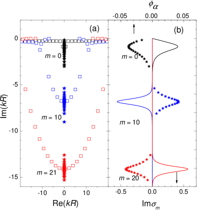
Figure 1: (a): Cut poles $k_{\alpha}$ (stars) representing the cut of the GF of a homogeneous dielectric cylinder with ${n_{r}}=2$, in the complex wave-number plane for $m=0$, 11, and 20. Normal poles $k_{n}$ (open squares) are also shown. (b): Cut pole density $\sigma_{m}(k)$ (solid curves) and the cut pole strength $\phi_{\alpha}^{(m)}$ (stars), for the same values of $m$.

I use the same method to discretised this continuum into cut poles $k_{\alpha}$ and cut pole strengths $\phi_{\alpha}^{(m)}$ as in my Ref.DoostPRA12

$$k_{\alpha}^{(m)}=\left.\int_{q_{\alpha}^{(m)}}^{q_{\alpha+1}^{(m)}}k\sigma_{m}(k)dk\right/\phi_{\alpha}^{(m)}$$ (45)

where the cut pole strength $\phi_{\alpha}^{(m)}$ is defined as

$$\phi_{\alpha}^{(m)}=\int_{q_{\alpha}^{(m)}}^{q_{\alpha+1}^{(m)}}\sigma_{m}(k)dk$$ (46)

An example of cut poles assigned for $m=0$, 10, and 20 is given in Fig. 1(a). The cut poles contribute to the RSE in the same way as the normal poles.

In the numerical calculation in Sec. V, I use $N_{c}^{(m)}\sim N^{(m)}$, where $N^{(m)}$ is the number of normal poles in the basis for the given $m$ and $N_{c}^{(m)}$ is the number of cut poles, in order to demonstrate the convergence towards the exact solution.

The next section discusses results of the RSE for different effective 2D systems. We consider a homogeneous dielectric cylinder of radius $R$ and refractive index $n_{r}=2$ ($\varepsilon=4$) with a homogeneous perturbation of the whole cylinder in Sec. V. Explicit forms of the matrix elements for these perturbations and details of their calculation are given in Appendix C.

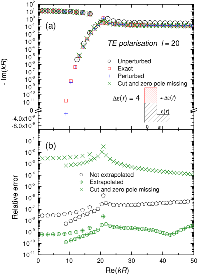
Figure 2: (a): Perturbed RS wave numbers for the homogeneous perturbation Eq. (47) calculated via the RSE with $N=800$ (only sine modes are shown). The perturbed poles with (+) and without ($\times$) the cut contribution are compared with the exact solution (open squares). Unperturbed wave numbers are also show (open circles with dots). Inset: Dielectric constant profile for the unperturbed and perturbed systems. (b): Relative error in the calculated perturbed wave numbers with (heptagons) and without (triangles) contribution of the cut. Relative error for a simulation including the cut and improved by extrapolation is also shown (crossed circles).

V Homogeneous Cylinder Perturbation

In this section I present my numerical results which support the validity of the analytic results relating to the $2$-dimensional TE RSE which I have provided in this manuscript.

The perturbation we consider in this section is a homogeneous change of $\varepsilon$ over the whole cylinder, given by

$$\Delta\varepsilon(\rho,\varphi)=\Delta\varepsilon\theta(R-\rho)=\left\{\begin{array}[]{cl}\Delta\varepsilon&\text{for\ \ }\rho\leqslant R\,,\\ 0&\text{for\ \ }\rho>R\end{array}\right.$$ (47)

with the strength $\Delta\varepsilon=4$ used in the numerical calculation. For $\varphi$-independent perturbations, modes with different azimuthal number $m$ are decoupled, and so are even and odd (cosine and sine). I show only the sine modes here, and use for illustration $m=20$. The matrix elements of the perturbation are calculated analytically and given by Eq. (12). The homogeneous perturbation does not change the symmetry of the system, so that the perturbed modes obey the same secular equation Eq. (34) with the refractive index $n_{r}$ of the cylinder changed to $\sqrt{n_{r}^{2}+\Delta\varepsilon}$, and thus the perturbed wave numbers $\varkappa_{\nu}$ calculated using the RSE can be compared with the exact values $\varkappa^{\rm(exact)}_{\nu}$.

We choose the basis of RSs for the RSE in such a way that for the given azimuthal number $m$ and the given number of normal RSs $N$ we find all normal poles $|k_{n}|<k_{\rm max}(N)$ with a suitably chosen maximum wave vector $k_{\rm max}(N)$ and then add the cut poles. We find that as we increase $N$, the relative error $\bigl{|}{\varkappa_{\nu}}/{\varkappa^{\rm(exact)}_{\nu}}-1\bigr{|}$ decreases as $N^{-3}$. Following the procedure described in Ref.DoostPRA12 we can extrapolate the perturbed wave numbers. The resulting perturbed wave numbers are shown in Fig. 2. The perturbation is strong, creating 3 additional WGMs with $m=20$ having up to 4 orders of magnitude narrower linewidths. For $N=800$, the RSE reproduces about 100 modes to a relative error in the $10^{-7}$ range, which is decreasing by one or two orders of magnitude after extrapolation. The contribution of the cut and zero frequency mode is significant: Ignoring these modes leads to a relative error of the poles in the $10^{-3}$ range. The fact that the relative error improves by 4-5 orders of magnitude after taking into account the cut in the form of the cut poles shows the validity of the reported analytical treatment of cuts in the RSE, and the high accuracy of the discretisation method into cut poles.

VI Summary

I have applied the resonant state expansion (RSE) to effective two-dimensional (2D) open optical systems, such as dielectric micro-cylinders and micro-disks with perturbations, by finding a formula linking the normalisation of resonant states appearing in the magnetic and electric Green’s functions which describe identical systems. These analytic formulas allow us to take advantage of an analytic Green’s function of the magnetic field of the homogeneous micro-cylinder to normalise the modes appearing in the spectral representation of the Green’s function for the electric field, electric modes which when normalised form the basis of the RSE.

Using the analytically known basis of resonant states (RSs) of an ideal homogeneous dielectric cylinder – a complete set of eigenmodes satisfying outgoing wave boundary conditions – I have treated an effectively 1D homogeneous perturbations. I investigated the convergence for this perturbations and compared the RSE with analytic solutions. I have found agreement between the RSE and analytic solutions.

Appendix A Normalised electric modes expressed in terms of normalised magnetic modes

In this appendix I provide the analytic formula relating the normalised $\mathbf{E}_{\bar{n}}$ and normalised $\mathbf{H}_{\bar{n}}$ modes. The basic principals of my derivation are as follows, let us consider the case where the $\bf\mathbf{E}$ and $\bf\mathbf{H}$ fields are both generated by a oscillating electric current $\bf\mathbf{J}$. By using an identical current to generate $\bf\mathbf{E}$ and $\bf\mathbf{H}$ fields and letting the current tend to zero as its harmonic wavenumber of oscillation tends to the resonant wavenumber $k_{\bar{n}}$ we can compare residues of $\hat{\mathbf{G}}^{H}_{k}$ and $\hat{\mathbf{G}}^{E}_{k}$ in order to relate normalised $\mathbf{E}_{\bar{n}}$ and $\mathbf{H}_{\bar{n}}$. The $\mathbf{H}_{\bar{n}}$ modes, including the continuum modes, discussed in Appendix B, can be normalised by comparing the residue of the spectral GF and the residue of the analytic GF, derived in Appendix B. The detailed mathematics will now be thoroughly explained.

Our starting point for finding a relation between the correct normalisation of the modes appearing in the spectral Green’s function for the magnetic $\mathbf{H(\mathbf{r})}$-field and electric $\mathbf{E(\mathbf{r})}$-field of a homogeneous dielectric micro-cylinder is Maxwell’s equations of electrodynamics,

$$\nabla\times\bf\mathbf{E}=ik{\bf H}\,,\ \ \ \ \ \nabla\times{\bf H}=-ik{\bf D}-{\bf J}$$ (48)

where we have assumed harmonic oscillation of the driving current with respect to time, so that the time derivative in Eq. (48) can be replaced with $ik$.

For the $\mathbf{E(\mathbf{r})}$-field with a current source $\mathbf{J(\mathbf{r})}$ oscillating at frequency $k$ we have according to Maxwell,

$$-\nabla\times\nabla\times\mathbf{E(\mathbf{r})}+k^{2}\varepsilon\mathbf{E(\mathbf{r})}=ik\mathbf{J(\mathbf{r})}$$ (49)

and also the corresponding wave equation with a source for the $\mathbf{H(\mathbf{r})}$-field,

$$-\nabla\times\nabla\times\mathbf{H(\mathbf{r})}+\dfrac{\nabla\varepsilon(\mathbf{r})}{\varepsilon(\mathbf{r})}\times(\nabla\times\mathbf{H(\mathbf{r})})+k^{2}\varepsilon(r)\mathbf{H(\mathbf{r})}\\ =\nabla\times\mathbf{J(\mathbf{r})}-\dfrac{\nabla\varepsilon(\mathbf{r})}{\varepsilon(\mathbf{r})}\times\mathbf{J(\mathbf{r})}$$ (50)

The GF for Eq. (49) is,

$$-\nabla\times\nabla\times\hat{\mathbf{G}}^{E}_{k}(\mathbf{r},\mathbf{r}^{\prime})+k^{2}\hat{\boldsymbol{\varepsilon}}({\bf r})\hat{\mathbf{G}}^{E}_{k}(\mathbf{r},\mathbf{r}^{\prime})=\hat{\mathbf{1}}\delta(\mathbf{r}-\mathbf{r}^{\prime})$$ (51)

and for Eq. (50)

$$-\nabla\times\nabla\times\hat{\mathbf{G}}^{H}_{k}(\mathbf{r},\mathbf{r}^{\prime})+{\hat{\boldsymbol{\varepsilon}}({\bf r})}^{-1}{\nabla\hat{\boldsymbol{\varepsilon}}({\bf r})}\times(\nabla\times\hat{\mathbf{G}}^{H}_{k}(\mathbf{r},\mathbf{r}^{\prime}))\\ +k^{2}\hat{\boldsymbol{\varepsilon}}({\bf r})\hat{\mathbf{G}}^{H}_{k}(\mathbf{r},\mathbf{r}^{\prime})\\ =\hat{\mathbf{1}}\delta(\mathbf{r}-\mathbf{r}^{\prime})$$ (52)

The formulas for the $\mathbf{E(\mathbf{r})}$-field and $\mathbf{H(\mathbf{r})}$-field in terms of their respective Green’s functions are given as the following convolutions with the source,

$$\mathbf{E(\mathbf{r})}=\int\hat{\mathbf{G}}^{E}_{k}(\mathbf{r},\mathbf{r}^{\prime})ik\mathbf{J(\mathbf{r})}d\mathbf{r}^{\prime}$$ (53)

$$\mathbf{H(\mathbf{r})}=\int\hat{\mathbf{G}}^{H}_{k}(\mathbf{r},\mathbf{r}^{\prime})\left[\nabla\times\mathbf{J(\mathbf{r}^{\prime})}-\dfrac{\nabla\varepsilon(\mathbf{r}^{\prime})}{\varepsilon(\mathbf{r}^{\prime})}\times\mathbf{J(\mathbf{r}^{\prime})}\right]d\mathbf{r}^{\prime}$$ (54)

Since at this stage $\mathbf{J(\mathbf{r})}$ is arbitrary we can set $\mathbf{J}(\mathbf{r})=0$ when $\rho>R_{-}$ where $R_{-}$ is some radius $R_{-}<R$. $R$ is the radius of the micro-cylinder. Also since we choose our basis system to be a homogeneous micro-cylinder, importantly for Eq. (58) $\nabla\varepsilon(\rho,\varphi)=0$ when $\rho<R$. At this stage $k$ is also arbitrary so let it be $k=k_{\bar{n}}+\Delta k$, $\Delta k\rightarrow 0$. To simplify our discussion let $\mathbf{W(r)}$ be a function related to $\mathbf{J(\mathbf{r})}$ by,

$$ik\mathbf{J}(\mathbf{r})=2k_{\bar{n}}\Delta k\mathbf{W(\mathbf{r})}$$ (55)

Eq. (55) allows $\mathbf{J(\mathbf{r})}$ to meet the requirements that I have just set out.

In light of Eq. (55) Eq. (53) becomes

$$\lim_{\Delta k\rightarrow 0}\int_{R_{-}}\left[\sum_{\bar{m}}\frac{\phi_{\bar{m}}\mathbf{E}_{\bar{m}}(\mathbf{r})\otimes\mathbf{E}_{\bar{m}}(\mathbf{r}^{\prime})}{2k_{\bar{m}}(k_{\bar{n}}-k_{\bar{m}}+\Delta k)}\right]2k_{\bar{n}}\Delta k\mathbf{W(r^{\prime})}d\mathbf{r}^{\prime}\\ =\phi_{\bar{n}}\mathbf{E_{\bar{n}}(\mathbf{r})}\int\mathbf{E}_{\bar{n}}(\mathbf{r}^{\prime})\cdot\mathbf{W(r^{\prime})}d\mathbf{r}^{\prime}=\mathbf{E(r)}$$ (56)

where we have replaced $\hat{\mathbf{G}}^{E}_{k}(\mathbf{r},\mathbf{r}^{\prime})$ with its spectral representation

$$\hat{\mathbf{G}}_{k}(\mathbf{r},\mathbf{r}^{\prime})=\hbox to0.0pt{$\displaystyle\sum_{n}$\hss}\int\,\frac{\mathbf{E}_{n}(\mathbf{r})\otimes\mathbf{E}_{n}(\mathbf{r}^{\prime})}{2k(k-k_{n})}\approx\sum_{\bar{n}}\frac{\phi_{\bar{n}}\mathbf{E}_{\bar{n}}(\mathbf{r})\otimes\mathbf{E}_{\bar{n}}(\mathbf{r}^{\prime})}{2k(k-k_{\bar{n}})}$$ (57)

Similarly Eq. (54) becomes

$$\mathbf{H(r)}=\lim_{\Delta k\rightarrow 0}\int_{R_{-}}\left[\sum_{\bar{m}}\frac{\phi_{\bar{m}}\mathbf{H}_{\bar{m}}(\mathbf{r})\otimes\mathbf{H}_{\bar{m}}(\mathbf{r}^{\prime})}{2k_{\bar{m}}(k_{\bar{n}}-k_{\bar{m}}+\Delta k)}\right]\\ \cdot\left[\dfrac{2k_{\bar{n}}\Delta k\nabla\times\mathbf{W(r^{\prime})}}{ik}\right]d\mathbf{r}^{\prime}\\ =\phi_{\bar{n}}\mathbf{H_{\bar{n}}(r)}\int_{R_{-}}\dfrac{\mathbf{H}_{\bar{n}}(\mathbf{r}^{\prime})\cdot(\nabla\times\mathbf{W(r^{\prime})})}{ik_{\bar{n}}}d\mathbf{r}^{\prime}$$ (58)

where we have replaced $\hat{\mathbf{G}}^{H}_{k}(\mathbf{r},\mathbf{r}^{\prime})$ with its spectral representation

$$\hat{\mathbf{G}}^{H}_{k}(\mathbf{r},\mathbf{r}^{\prime})=\sum_{n}\frac{\phi_{\bar{n}}\mathbf{H}_{\bar{n}}(\mathbf{r})\otimes\mathbf{H}_{\bar{n}}(\mathbf{r}^{\prime})}{2k(k-k_{\bar{n}})}$$ (59)

Eq. (58) and Eq. (56) can be substituted in Eq. (48) to give,

$$\left[\nabla\times\mathbf{\mathbf{E}_{\bar{n}}(\mathbf{r})}\right]\int_{R_{-}}\mathbf{E}_{\bar{n}}(\mathbf{r}^{\prime})\cdot\mathbf{W(r^{\prime})}d\mathbf{r}^{\prime}\\ =\mathbf{\mathbf{H}_{\bar{n}}(r)}\int_{R_{-}}\mathbf{H}_{\bar{n}}(\mathbf{r}^{\prime})\cdot(\nabla\times\mathbf{W(r^{\prime})})d\mathbf{r}^{\prime}$$ (60)

We now make the substitution $\mathbf{W(\mathbf{r})}=\Gamma(\rho)\mathbf{\mathbf{E}_{\bar{n}}(\mathbf{r})}$, where,

$$\Gamma(\rho)=\left\{\begin{array}[]{cl}1&\text{for\ \ }\rho\leqslant R_{-}\,,\\ 0&\text{for\ \ }\rho>R_{-}\end{array}\right.$$ (61)

We can calculate the curl of $\mathbf{W(\mathbf{r})}$ analytically. First note for a given mode we can evaluate Eq. (48) to be equivalently (in this case)

$$\nabla\times\mathbf{E}_{\bar{n}}(\mathbf{r})=\dfrac{n^{2}_{r}\mathbf{H}_{\bar{n}}(\mathbf{r})}{M_{k_{\bar{n}}}}$$ (62)

where ${M_{k_{\bar{n}}}}$ is an unknown to be found.

Using Eq. (62) we can write the following identity for $\mathbf{W(\mathbf{r})}$:

$$\nabla\times\mathbf{W(\mathbf{r})}=\nabla\Gamma(\rho)\times\mathbf{E}_{\bar{n}}(\mathbf{r})+\Gamma(\rho)\nabla\times\mathbf{E}_{\bar{n}}(\mathbf{r})\\ =-\delta(\rho-R_{-})e_{\rho}\times\mathbf{\mathbf{E}_{\bar{n}}(\mathbf{r})}+\Gamma(\rho)\dfrac{n^{2}_{r}\mathbf{H}_{\bar{n}}(\mathbf{r})}{M_{k_{\bar{n}}}}$$ (63)

Substituting Eq. (63) into Eq. (60) and cancelling common factors of $\mathbf{H}_{\bar{n}}(\mathbf{r})$ gives

$$\left[\dfrac{n^{2}_{r}}{M_{k_{\bar{n}}}}\right]\int_{R_{-}}\mathbf{E}_{\bar{n}}(\mathbf{r}^{\prime})^{2}d\mathbf{r}^{\prime}\\ =-\int_{R_{-}}\mathbf{H}_{\bar{n}}(\mathbf{r}^{\prime})\cdot\delta(\rho^{\prime}-R_{-})e_{\rho}\times\mathbf{\mathbf{E}_{\bar{n}}(\mathbf{r}^{\prime})}d\mathbf{r}^{\prime}+\\ +\int_{R_{-}}\Gamma(\rho^{\prime})\dfrac{n^{2}_{r}\left[\mathbf{H}_{\bar{n}}(\mathbf{r}^{\prime})\right]^{2}}{M_{k_{\bar{n}}}}d\mathbf{r}^{\prime}$$ (64)

Substituting Eq. (40) into Eq. (64)

$$\int_{R_{-}}\mathbf{E}_{\bar{n}}(\mathbf{r}^{\prime})^{2}d\mathbf{r}^{\prime}\\ =\int^{\pi}_{-\pi}R_{-}d\varphi\chi_{m}(\varphi)\chi_{m}(\varphi)\cdot\dfrac{A^{2}_{\bar{n}}J_{m}(nk_{\bar{n}}R_{-})}{k^{2}_{\bar{n}}n^{2}_{r}}\dfrac{\partial{J_{m}(nk_{\bar{n}}R_{-})}}{\partial{\rho}}\\ +\int_{R_{-}}\mathbf{H}_{\bar{n}}(\mathbf{r}^{\prime})^{2}d\mathbf{r}^{\prime}$$ (65)

Eq. (40) was generated by Eq. (68), where $M_{k_{\bar{n}}}$ is the unknown we are trying to find. In Eq. (65) we took

$$\mathbf{H}_{\bar{n}}(\mathbf{r})=A_{\bar{n}}J_{m}(nk_{\bar{n}}\rho)\chi_{m}(\varphi){{\bf e}_{z}}$$ (66)

and re-calculated $\mathbf{E}_{\bar{n}}$ according to Eq. (68).

Calculating the first integral in Eq. (65) by making substitutions from Eq. (40)

$$\int_{R_{-}}\mathbf{E}_{\bar{n}}(\mathbf{r}^{\prime})^{2}d\mathbf{r}^{\prime}\\ =\dfrac{A(k_{\bar{n}})^{2}}{{M^{2}_{k_{\bar{n}}}}k^{4}_{\bar{n}}}\int_{R_{-}}\left[\dfrac{m^{2}J^{2}_{m}(nk_{\bar{n}}\rho^{\prime})}{\rho^{\prime}}+\rho^{\prime}\left[\dfrac{\partial{J_{m}(nk_{\bar{n}}\rho^{\prime})}}{\partial{\rho}}\right]^{2}\right]d\rho^{\prime}$$ (67)

having made use of

$$\nabla\times\mathbf{H}_{\bar{n}}(\mathbf{r})=M_{k_{\bar{n}}}k^{2}_{\bar{n}}\mathbf{E}_{\bar{n}}(\mathbf{r})$$ (68)

which comes from taking the curl of Eq. (62) and using the definition of RSs, specifically, inside the homogenous cylinder,

$$\nabla\times\nabla\times\mathbf{E}_{\bar{n}}(\mathbf{r})=k^{2}_{\bar{n}}n^{2}_{r}\mathbf{E}_{\bar{n}}(\mathbf{r})$$ (69)

Eq. (67) is not instantly recognisable as a standard integral, however if we make use of the two following general properties of Bessel function,

$$J_{m-1}(z)-J_{m+1}(z)=2{J}_{m}^{\prime}(z)$$ (70)

$$J_{m-1}(z)+J_{m+1}(z)=\dfrac{2m}{z}{J}_{m}(z)$$ (71)

we see that

$$\int_{R_{-}}\mathbf{E}_{\bar{n}}(\mathbf{r}^{\prime})^{2}d\mathbf{r}^{\prime}\\ =\dfrac{A(k_{\bar{n}})^{2}n^{2}_{r}}{2M^{2}_{k_{\bar{n}}}k^{2}_{\bar{n}}}\int_{R_{-}}\left[J^{2}_{m-1}(n_{r}k_{\bar{n}}\rho^{\prime})+J^{2}_{m+1}(n_{r}k_{\bar{n}}\rho^{\prime})\right]\rho^{\prime}d\rho^{\prime}$$ (72)

which is a standard integral given in Appendix C.

In the last integral in Eq. (65) we can make substitutions from Eq. (IV) and Eq. (IV) to obtain the following standard integral given in Appendix C,

$$\int_{R_{-}}\mathbf{H}_{\bar{n}}(\mathbf{r}^{\prime})^{2}d\mathbf{r}^{\prime}=A(k_{\bar{n}})^{2}\int_{R_{-}}J^{2}_{m}(nk_{\bar{n}}\rho^{\prime})\rho^{\prime}d\rho^{\prime}$$ (73)

Finally we use Eq. (72) and Eq. (73) to solve Eq. (65) for $M_{k_{\bar{n}}}$

$$\dfrac{2{M^{2}_{k_{\bar{n}}}}}{n^{4}_{r}}=\\ =\dfrac{\int\left[J^{2}_{m-1}(n_{r}k_{\bar{n}}\rho^{\prime})+J^{2}_{m+1}(n_{r}k_{\bar{n}}\rho^{\prime})\right]\rho^{\prime}d\rho^{\prime}}{R_{-}J_{m}(n_{r}k_{\bar{n}}R_{-})\dfrac{\partial{J_{m}(n_{r}k_{\bar{n}}R_{-})}}{\partial{r}}+k^{2}_{\bar{n}}\varepsilon\int J^{2}_{m}(nk_{\bar{n}}\rho^{\prime})\rho^{\prime}d\rho^{\prime}}\\ =\dfrac{2}{n^{2}_{r}k^{2}_{\bar{n}}}$$ (74)

or

$$M^{2}_{k_{\bar{n}}}=\dfrac{n^{2}_{r}}{k^{2}_{\bar{n}}}$$ (75)

I evaluate analytically the integral in Eq. (74) in Appendix D.

Hence our analytics in this section have reached their conclusion. We can now mathematically relate normalised $\mathbf{E}_{\bar{n}}$ modes to normalised $\mathbf{H}_{\bar{n}}$ modes with the analytic formula,

$$\nabla\times\mathbf{H}_{\bar{n}}(\mathbf{r})=M_{k_{\bar{n}}}k^{2}_{\bar{n}}\mathbf{E}_{\bar{n}}(\mathbf{r})$$ (76)

I make use of this valuable derived Eq. (76) in Appendix B, Sec. III, Sec. IV and Sec. V, to translate the correctly normalised $\mathbf{H}_{\bar{n}}$ modes therein derived, into correctly normalised $\mathbf{E}_{\bar{n}}$ modes.

Appendix B Green’s function of a homogeneous cylinder

In this appendix I nearly exactly repeat the derivation I made with E. A. Muljarov in Ref.DoostPRA13 and derive an analytic GF for $2$-dimensional cylindrical homogeneous electromagnetic resonators.

The only difference between the analytics here and the analytics of Appendix B Ref.DoostPRA13 is that here I am restricted to the magnetic $\bf\mathbf{H}$-field GF of the $2$-dimensional TE modes of the cylinder, while in Appendix B of Ref.DoostPRA13 we were restricted to the $\bf\mathbf{E}$-field TM modes of a mathematically identical system.

The reason for the difference in approach between this appendix and Ref.DoostPRA13 is that to formulate the $\bf\mathbf{E}$-field TE modes into effectively $1$-dimensional equations is currently an unsolved problem. To generate the analytic GF of the electrodynamic problem, using the methods in this appendix, requires the recasting of the equation into a set of decoupled $1$-dimensional problems.

The TE component of the GF of a homogeneous cylinder in vacuum satisfies the following equation for magnetic field

$$-\nabla\times\nabla\times\hat{\mathbf{G}}^{H}_{k}(\mathbf{r},\mathbf{r}^{\prime})+\dfrac{\nabla\varepsilon({\bf r})}{\varepsilon({\bf r})}\times(\nabla\times\hat{\mathbf{G}}^{H}_{k}(\mathbf{r},\mathbf{r}^{\prime}))\\ +k^{2}\varepsilon({\bf r})\hat{\mathbf{G}}^{H}_{k}(\mathbf{r},\mathbf{r}^{\prime})=\hat{\mathbf{1}}\delta(\mathbf{r}-\mathbf{r}^{\prime})$$ (77)

with

$$\varepsilon(\rho)=\left\{\begin{array}[]{lll}n_{r}^{2}&{\rm for}&\rho\leqslant R\,,\\ 1&{\rm for}&\rho>R\end{array}\right.$$ (78)

Using the angular basis Eq. (26) the GF can be written as

$$G^{H}_{k}(\mbox{\boldmath${\rho}$},\mbox{\boldmath${\rho}$}^{\prime})=\frac{1}{\sqrt{\rho\rho^{\prime}}}\sum_{m}\tilde{G}^{H}_{m}(\rho,\rho^{\prime};k)\chi_{m}(\varphi)\chi_{m}(\varphi^{\prime})$$ (79)

similar to Eq. (42). Note that we redefined here the radial part as $\tilde{G}^{H}_{m}(\rho,\rho^{\prime};k)=\sqrt{\rho\rho^{\prime}}{G}^{H}_{m}(\rho,\rho^{\prime};k)$ which satisfies

$$\left[\frac{d^{2}}{d\rho^{2}}-\frac{m^{2}-1/4}{\rho^{2}}+\dfrac{1}{\varepsilon(\rho)}\dfrac{d\varepsilon(\rho)}{d\rho}\dfrac{1}{2\rho}\right]\tilde{G^{H}}_{m}(\rho,\rho^{\prime};k)+\\ +\left[k^{2}\varepsilon(\rho)-\dfrac{1}{\varepsilon(\rho)}\dfrac{d\varepsilon(\rho)}{d\rho}\frac{d}{d\rho}\right]\tilde{G^{H}}_{m}(\rho,\rho^{\prime};k)=\delta(\rho-\rho^{\prime})$$ (80)

Using two linearly independent solutions $f_{m}(\rho)$ and $g_{m}(\rho)$ of the corresponding homogeneous equation which satisfy the asymptotic boundary conditions

$$\begin{array}[]{lll}f_{m}(\rho)\propto\rho^{m+1/2}&{\rm for}&\rho\to 0\,,\\ g_{m}(\rho)\propto e^{ik\rho}&{\rm for}&\rho\to\infty\end{array}$$

the GF can be expressed as

$$\tilde{G^{H}}_{m}(\rho,\rho^{\prime};k)=\frac{f_{m}(\rho_{<})g_{m}(\rho_{>})}{W(f_{m},g_{m})}$$ (81)

in which $\rho_{<}=\min\{\rho,\rho^{\prime}\}$, $\rho_{>}=\max\{\rho,\rho^{\prime}\}$, and the Wronskian $W(f,g)=fg^{\prime}-f^{\prime}g$ . For TE polarization, a suitable pair of solutions is given by

$$f_{m}(\rho) = \sqrt{\rho}\cdot\left\{\begin{array}[]{ll}J_{m}(n_{r}\rho k)\,,&\rho\leqslant R\,,\\ a_{m}J_{m}(\rho k)+b_{m}H_{m}(\rho k)\,,&\rho>R\end{array}\right.$$ (84)

$$g_{m}(\rho) = \sqrt{\rho}\cdot\left\{\begin{array}[]{ll}c_{m}J_{m}(n_{r}\rho k)+d_{m}H_{m}(n_{r}\rho k)\,,&\rho\leqslant R\,,\\ H_{m}(\rho k)\,,&\rho>R\end{array}\right.$$ (87)

where

$$a_{m}(k) = \bigl{[}H_{m}(x)J_{m}^{\prime}(n_{r}x)-n_{r}H_{m}^{\prime}(x)J_{m}(n_{r}x)\bigr{]}\pi ix/2n_{r}\,,$$

$$b_{m}(k) = \bigl{[}n_{r}J_{m}^{\prime}(x)J_{m}(n_{r}x)-J_{m}(x)J_{m}^{\prime}(n_{r}x)\bigr{]}\pi ix/2n_{r}\,,$$

$$c_{m}(k) = \bigl{[}n_{r}H_{m}^{\prime}(x)H_{m}(n_{r}x)-H_{m}(x)H_{m}^{\prime}(n_{r}x)\bigr{]}\pi in_{r}x/2\,,$$

$$d_{m}(k) = \bigl{[}H_{m}(x)J_{m}^{\prime}(n_{r}x)-n_{r}H_{m}^{\prime}(x)J_{m}(n_{r}x)\bigr{]}\pi in_{r}x/2$$

with $x=kR$. The Wronskian is calculated to be

$$W(f_{m},g_{m})=2in^{2}_{r}a_{m}(k)=-nxD_{m}(x)/\pi,$$ (88)

with $D_{m}(x)$ defined in Eq. (36). Inside the cylinder, the GF then takes the form

$$\tilde{G^{H}}_{m}(\rho,\rho^{\prime};k) = \frac{\pi}{2i}\sqrt{\rho\rho^{\prime}}\biggl{[}J_{m}(n_{r}k\rho_{<})H_{m}(n_{r}k\rho_{>})$$ (89)

$$\left.-\frac{c_{m}(k)}{a_{m}(k)}J_{m}(n_{r}k\rho_{<})J_{m}(n_{r}k\rho_{>})\right]$$

The GF has simple poles $k_{n}$ in the complex $k$-plane which are the wave vectors of RSs, given by $a_{m}(k_{n})=0$, an equation equivalent to Eq. (34). The residues ${\rm Res}_{n}$ of the GF at these poles are calculated using

$$r_{m}(k_{n})=\left.-\frac{c_{m}(k)}{\frac{d}{dk}a_{m}(k)}\right|_{k=k_{n}}\\ =\frac{2i}{\pi(n^{2}_{r}-1)\left[\dfrac{m^{2}}{k_{n}}\left[J_{m}(nk_{n}R)\right]^{2}+R^{2}k_{n}\left[J^{\prime}_{m}(nk_{n}R)\right]^{2}\right]}$$ (90)

which can be seen by noting that inside the resonantor Eq. (81) and Eq. (59) are equal as $k\rightarrow k_{n}$ as they are equal for all $k$, at every point in space inside the resonator.

In addition to the poles, the GF has a cut in the complex $k$-plane along the negative imaginary half-axis. The cut is due to the Hankel function $H_{m}(z)$.

Owing to the cut of the Hankel function $H_{m}(z)$ the GF also has a cut along the negative imaginary half-axis in the complex $k$-plane, so that on both sides of the cut $\tilde{G}_{m}$ takes different values: $\tilde{G}^{+}_{m}$ one the right-hand side and $\tilde{G}^{-}_{m}$ one the left-hand side of the cut. The step $\Delta\tilde{G}_{m}=\tilde{G}^{+}_{m}-\tilde{G}^{-}_{m}$ over the cut can be calculated using the corresponding difference in the Hankel function:

$$\Delta H_{m}(z)=H^{+}_{m}(z)-H^{-}_{m}(z)=4J_{m}(z)$$

The result is

$$\Delta\tilde{G^{H}}_{m}(\rho,\rho^{\prime};k)=\frac{\pi}{2i}\sqrt{\rho\rho^{\prime}}J_{m}(n_{r}k\rho_{<})J_{m}(n_{r}k\rho_{>})\Delta Q_{m}(k)$$ (91)

where

$$\Delta Q_{m}(k)=\left[4-\frac{c_{m}^{+}}{a_{m}^{+}}+\frac{c_{m}^{-}}{a_{m}^{-}}\right]=-\left(\frac{4}{\pi kR}\right)^{2}\frac{1}{D_{m}^{+}(k)D_{m}^{-}(k)}$$ (92)

with $D_{m}(k)$ given by Eq. (36).

$$\oint\frac{\tilde{G^{H}}_{m}(\rho,\rho^{\prime};k^{\prime})}{k-k^{\prime}}dk^{\prime}=\int^{-i\infty}_{0}\frac{\tilde{G^{H}}^{+}_{m}dk^{\prime}}{k-k^{\prime}}+\int_{-i\infty}^{0}\frac{\tilde{G^{H}}^{-}_{m}dk^{\prime}}{k-k^{\prime}}$$

$$=2\pi i\sum_{n}\frac{{\rm Res}_{n}}{k-k_{n}}-2\pi i\tilde{G^{H}}_{m}(\rho,\rho^{\prime};k)$$ (93)

Note that in second part of the above equation we have made use of the residue theorem, expressing the closed-loop integral in the left-hand side in terms of a sum over residues at all poles inside the contour. Using Eq. (93) the GF can be expressed as

$$\tilde{G}^{H}_{m}(\rho,\rho^{\prime};k)=\sum_{n}\frac{{\rm Res}_{n}}{k-k_{n}}+\frac{1}{2\pi i}\int_{-i\infty}^{0}\frac{\Delta\tilde{G}^{H}_{m}(\rho,\rho^{\prime};k^{\prime})dk^{\prime}}{k-k^{\prime}}$$ (94)

which is a generalization of the Mittag-Leffler theorem.

In conclusion then, the residues ${\rm Res}_{n}$ of the GF contributing to Eq. (94) are calculated as

$${\rm Res}_{n}=\frac{\pi}{2i}\sqrt{\rho\rho^{\prime}}J_{m}(n_{r}k\rho_{<})J_{m}(n_{r}k\rho_{>})r_{m}(k_{n})$$ (95)

with $r_{m}(k_{n})$ found in Eq. (90). Given that the spatial dependence of the GF, as described by Eqs. (94), (95), and (91), is represented by products of the RS wave functions $R_{m}(\rho,k_{n})$ and their analytic continuations $R_{m}(\rho,k)$ with $k$-values taken on the cut, we arrive at the GF in the form of Eqs.(43) and (44) which are then used in the RSE, once the modes have been converted into $\mathbf{E}_{\bar{n}}$ form using the analytics in appendix A.

Appendix C Homogeneous cylinder perturbation

In this appendix is given the perturbation matrix elements for the homogeneous perturbation of the TE modes of a homogeneous cylinder. I give the analytic expression for the perturbation matrix elements required to produce the numerical results in Sec. V, numerical results which validate the analytics which I developed for this manuscript.

The homogeneous perturbation Eq. (47) does not mix different angular momentum $m$-values. The matrix elements between RS with the same azimuthal number $m$ are given by the radial overlap integrals

$$V_{\bar{n}\bar{n}^{\prime}}=\dfrac{\hat{A}^{\rm TE}(k_{\bar{n}})\hat{A}^{\rm TE}(k_{\bar{n}^{\prime}})\gamma(k_{\bar{n}})\gamma(k_{\bar{n}^{\prime}})\Delta\epsilon}{2}\\ \times\left[I_{m-1}(k_{\bar{n}},k_{\bar{n}^{\prime}})+I_{m+1}(k_{\bar{n}},k_{\bar{n}^{\prime}})\right]\,$$ (96)

where,

$$\gamma(k_{\bar{n}})=\left\{\begin{array}[]{cl}\sqrt{|m|(n^{2}_{r}-1)}&\text{for\ \ }k_{\bar{n}}=0\,,\\ 1&\text{otherwise\ \ }\end{array}\right.$$ (97)

and

$$I_{j}(k_{\bar{n}},k_{\bar{n}^{\prime}})=\int_{R}J_{j}(nk_{\bar{n}}\rho^{\prime})J_{j}(nk_{\bar{n}^{\prime}}\rho^{\prime})\rho^{\prime}d\rho^{\prime}$$ (98)

yielding for identical basis states ($\bar{n}=\bar{n}^{\prime}$)

$$I_{m}(k_{\bar{n}},k_{\bar{n}^{\prime}})\\ =\frac{R^{2}}{2}\left[[J_{m}(n_{r}k_{\bar{n}}R)]^{2}-J_{m-1}(n_{r}k_{\bar{n}}R)J_{m+1}(n_{r}k_{\bar{n}}R)\right]$$ (99)

and for different basis states ($\bar{n}\neq\bar{n}^{\prime}$)

$$\dfrac{R}{k^{2}_{\bar{n}}-k^{2}_{\bar{n}^{\prime}}}\cdot\dfrac{k_{\bar{n}^{\prime}}}{n_{r}}J_{m}(k_{\bar{n}}n_{r}R)J_{m-1}(k_{\bar{n}^{\prime}}n_{r}R)\\ -\dfrac{R}{k^{2}_{\bar{n}}-k^{2}_{\bar{n}^{\prime}}}\cdot\dfrac{k_{\bar{n}}}{n_{r}}J_{m}(k_{\bar{n}^{\prime}}n_{r}R)J_{m-1}(k_{\bar{n}}n_{r}R)\\ =I_{m}(k_{\bar{n}},k_{\bar{n}^{\prime}})$$ (100)

When $k_{\bar{n}}=0$ we can use the asymptotic form of the Bessel function,

$$J_{m}(z)=\dfrac{(z/2)^{m}}{\Gamma(m+1)}$$ (101)

$$\Gamma(m+1)=m!$$ (102)

from which we see $k_{\bar{n}}\rightarrow 0$ cancels out everywhere in $V_{\bar{n}\bar{n}^{\prime}}$.

There is an important transformation to note,

$$\dfrac{{A}^{\rm TE}(k_{\bar{n}})}{J_{m}(k_{\bar{n}}n_{r}R)}=\hat{A}^{\rm TE}(k_{\bar{n}})$$ (103)

Hence with the analytic integrals in this appendix we are able to completely reproduce the analytic results in Sec. V.

Appendix D Evaluating Equation A26

In this appendix I analytically evaluate the important integral equation Eq. (74)

$$\dfrac{2{M^{2}_{k_{\bar{n}}}}}{n^{4}_{r}}=\\ =\dfrac{\int\left[J^{2}_{m-1}(n_{r}k_{\bar{n}}\rho^{\prime})+J^{2}_{m+1}(n_{r}k_{\bar{n}}\rho^{\prime})\right]\rho^{\prime}d\rho^{\prime}}{R_{-}J_{m}(n_{r}k_{\bar{n}}R_{-})\dfrac{\partial{J_{m}(n_{r}k_{\bar{n}}R_{-})}}{\partial{r}}+k^{2}_{\bar{n}}\varepsilon\int J^{2}_{m}(nk_{\bar{n}}\rho^{\prime})\rho^{\prime}d\rho^{\prime}}\\ =\dfrac{2}{n^{2}_{r}k^{2}_{\bar{n}}}$$ (104)

In order to evaluate Eq. (105) let us consider the numerator in the above integral, taking into account standard integrals,

$$2\int^{R}_{0}\left[J^{2}_{m-1}(n_{r}k_{\bar{n}}\rho^{\prime})+J^{2}_{m+1}(n_{r}k_{\bar{n}}\rho^{\prime})\right]\rho^{\prime}d\rho^{\prime}\\ =\left(R^{2}-\left(\dfrac{m-1}{k_{n}n_{r}}\right)^{2}\right)J^{2}_{m-1}(n_{r}k_{\bar{n}}R)+R^{2}\left[J_{m-1}^{\prime}(n_{r}k_{\bar{n}}R)\right]^{2}\\ +\left(R^{2}-\left(\dfrac{m+1}{k_{n}n_{r}}\right)^{2}\right)J^{2}_{m-1}(n_{r}k_{\bar{n}}R)+R^{2}\left[J_{m+1}^{\prime}(n_{r}k_{\bar{n}}R)\right]^{2}$$ (105)

with rearrangement and use of the following identities

$$J_{m-1}(z)-J_{m+1}(z)=2{J}_{m}^{\prime}(z)$$ (106)

$$J_{m-1}(z)+J_{m+1}(z)=\dfrac{2m}{z}{J}_{m}(z)$$ (107)

we arrive at,

$$\int^{R}_{0}\left[J^{2}_{m-1}(n_{r}k_{\bar{n}}\rho^{\prime})+J^{2}_{m+1}(n_{r}k_{\bar{n}}\rho^{\prime})\right]\rho^{\prime}d\rho^{\prime}\\ =\dfrac{R^{2}}{2}\left[J^{2}_{m-1}(n_{r}k_{\bar{n}}R)+J^{2}_{m+1}(n_{r}k_{\bar{n}}R)\right]\\ -\dfrac{R^{2}J_{m}(n_{r}k_{\bar{n}}R)}{n_{r}k_{\bar{n}}R}\left[\left(m-1\right)J_{m-1}(n_{r}k_{\bar{n}}R)+\left(m+1\right)J_{m+1}(n_{r}k_{\bar{n}}R)\right]\\ +J^{2}_{m}(n_{r}k_{\bar{n}}R)R^{2}$$ (108)

Further use of the identities Eq. (106), Eq. (107) and rearrangement gives

$$\int^{R}_{0}\left[J^{2}_{m-1}(n_{r}k_{\bar{n}}\rho^{\prime})+J^{2}_{m+1}(n_{r}k_{\bar{n}}\rho^{\prime})\right]\rho^{\prime}d\rho^{\prime}\\ =\dfrac{R^{2}}{2m}\left[J^{2}_{m-1}(n_{r}k_{\bar{n}}R)-J^{2}_{m+1}(n_{r}k_{\bar{n}}R)\right]\\ -R^{2}J_{m+1}(n_{r}k_{\bar{n}}R)J_{m-1}(n_{r}k_{\bar{n}}R)\\ +\dfrac{(n_{r}k_{\bar{n}}R)^{2}}{4m^{2}}\left[J_{m-1}(n_{r}k_{\bar{n}}R)+J_{m+1}(n_{r}k_{\bar{n}}R)\right]^{2}$$ (109)

Next we move on to the denominator

$$={RJ_{m}(n_{r}k_{\bar{n}}R)\dfrac{\partial{J_{m}(n_{r}k_{\bar{n}}R)}}{\partial{\rho}}+k^{2}_{\bar{n}}\varepsilon\int^{R}_{0}J^{2}_{m}(nk_{\bar{n}}\rho^{\prime})\rho^{\prime}d\rho^{\prime}}\\ =\dfrac{(n_{r}k_{\bar{n}}R)^{2}}{4m}\left[J^{2}_{m-1}(n_{r}k_{\bar{n}}R)-J^{2}_{m+1}(n_{r}k_{\bar{n}}R)\right]\\ +\dfrac{(n_{r}k_{\bar{n}}R)^{4}}{8m^{2}}\left[J_{m-1}(n_{r}k_{\bar{n}}R)+J_{m+1}(n_{r}k_{\bar{n}}R)\right]^{2}\\ -\dfrac{(n_{r}k_{\bar{n}}R)^{2}}{2}J_{m-1}(n_{r}k_{\bar{n}}R)J_{m+1}(n_{r}k_{\bar{n}}R)$$ (110)

where again I have made use of standard integrals, the identities Eq. (106), Eq. (107) and rearrangement.

Hence making use of these evaluations we arrive at the important result,

$$\dfrac{2{M^{2}_{k_{\bar{n}}}}}{n^{4}_{r}}=\\ =\dfrac{\int\left[J^{2}_{m-1}(n_{r}k_{\bar{n}}\rho^{\prime})+J^{2}_{m+1}(n_{r}k_{\bar{n}}\rho^{\prime})\right]\rho^{\prime}d\rho^{\prime}}{R_{-}J_{m}(n_{r}k_{\bar{n}}R_{-})\dfrac{\partial{J_{m}(n_{r}k_{\bar{n}}R_{-})}}{\partial{r}}+k^{2}_{\bar{n}}\varepsilon\int J^{2}_{m}(nk_{\bar{n}}\rho^{\prime})\rho^{\prime}d\rho^{\prime}}\\ =\dfrac{2}{n^{2}_{r}k^{2}_{\bar{n}}}$$ (111)

or

$$M^{2}_{k_{\bar{n}}}=\dfrac{n^{2}_{r}}{k^{2}_{\bar{n}}}$$ (112)

Where $M^{2}_{k_{\bar{n}}}$ is the factor that links $\mathbf{E}_{\bar{n}}$ to $\mathbf{H}_{\bar{n}}$ in Eq. (76).

Appendix E Rotating the cut

In this section I explain how to find the correct sheet of the Hankel function, this corresponds to rotating the cut in the Hankel function on the complex plane. The correct sheet of the Hankel function gives purely outgoing plane cylindrical waves, infinitely far from the resonator.

First of all let us consider how the Hankel function is defined. The Hankel function can be expressed as Gradshtein

$$H_{m}(z)=J_{m}(z)+iN_{m}(z)$$ (113)

using a multiple-valued Neumann function

$$N_{m}(z)=\tilde{N}_{m}(z)+\frac{2}{\pi}J_{m}(z)\ln\frac{z}{2}$$ (114)

where $\tilde{N}_{m}(z)=z^{m}F_{m}(z^{2})$ is a single-valued polynomial Gradshtein while $\ln z$ is a multiple-valued function defined on an infinite number of Riemann sheets.

However considering Eq. (114), since we know,

$$\ln\frac{z}{2}=\ln\frac{ze^{i2\pi M}}{2}=\ln\frac{z}{2}+2\pi Mi$$ (115)

where $M$ is an integer, we can also say that,

$$H_{m}(z)=\left[J_{m}(z)+iN_{m}(z)\right]-4MJ_{m}(z)$$ (116)

Hence by Eq. (116) we can add any multiple of $4J_{m}(z)$ to $H_{m}(z)$ and still obtain a valid solution to the following defining equation

$$\left[\dfrac{\partial^{2}}{\partial\rho^{2}}+\dfrac{1}{\rho}\dfrac{\partial}{\partial\rho}-\dfrac{m^{2}}{\rho^{2}}+k^{2}\right]H_{m}(\rho k)=0$$ (117)

Let us investigate the meaning of this result further. Since

$$\lim_{\rho\rightarrow\infty}J_{m}(\rho k)={\sqrt{\dfrac{2}{\pi k\rho}}}\left({e^{i\rho k}+e^{-i\rho k}}\right)$$ (118)

we can see from Eq. (116) that changing the value of the integer $M$ corresponds to altering the boundary condition for the solution of Eq. (117) such that as $M\rightarrow\infty$ we have an equal balance between incoming and outgoing waves, infinitely far from the cylinder.

Hence in order to find the Hankel function with the correct boundary conditions we must consider the general solution to Eq. (117) in the limit of $\rho\rightarrow\infty$, where Eq. (117) becomes

$$\left[\dfrac{\partial^{2}}{\partial\rho^{2}}+\dfrac{1}{\rho}\dfrac{\partial}{\partial\rho}+k^{2}\right]H_{m}(\rho k)=0$$ (119)

and

$$\lim_{\rho\rightarrow\infty}H_{m}(\rho k)={\sqrt{\dfrac{2}{\pi k\rho}}}\left({Ae^{-i\rho k}+Be^{+i\rho k}}\right)$$ (120)

is the sum of incoming and outgoing plane waves.

We require in Eq. (120) $A=0$. We achieve this by first calculating the ratio $A/B$ and then adding or subtracting multiples of $4J_{m}(\rho k)$ to $H_{m}(\rho k)$ in order to obtain a solution with the correct boundary conditions.

The calculation of $A/B$ is as follows,

$$\lim_{\rho\rightarrow\infty}\dfrac{H_{m}(-\rho k_{n})}{H_{m}(+\rho k_{n})}=\dfrac{Ae^{+i\rho k_{n}}+Be^{-i\rho k_{n}}}{Ae^{-i\rho k_{n}}+Be^{+i\rho k_{n}}}=\dfrac{A}{B}$$ (121)

noting $\Im(k_{n})\leq 0$. If $A/B=0$ we have the correct sheet of the Hankel function. The Eq. (121) should be evaluated numerically on the computer for large values of $\rho$, convergence will be quick due to the exponential nature of the functions involved.

Hence I have formulated a numerical recipe to rotate the cut and find the correct sheet of the Hankel function. The correct sheet of the Hankel function is the sheet which provides us with outgoing boundary condition for use in the calculation of the RS eigenmodes (see pairs Eq. (33) and Eq. (35), Eq. (34) and Eq. (36)).

References

(1) V. B. Braginsky, M. L. Gorodetsky, V. S. Ilchenko, Phys. Lett. A 137, 393-397 (1989).
(2) K. J. Vahala, Nature (London) 424 (2003) 839.
(3) J. U. Nockel, A. D. Stone, Nature (London) 385 (1997) 45
(4) C. Gmachl, F. Capasso, E. E. Narimanov, J. U. Nockel, A. D. Stone, J. Faist, D. L. Sivco, A. Y. Cho, Science 280 (1998) 1556.
(5) S. B. Lee, J. H. Lee, J. S. Chang, H. J. Moon, S. W. Kim, K. An, Phys. Rev. Lett. 88 (2002) 033903.
(6) T. Harayama, T. Fukushima, P. Davis, P. O. Vaccaro, T. Miyasaka, T. Nishimura, T. Aida, Phys. Rev. E 67 (2003) 015207(R)
(7) G. D. Chern, H. E. Tureci, A. D. Stone, R. K. Chang, M. Kneissl, N. M. Johnson, Appl. Phys. Lett. 83 (2003) 1710.
(8) M. S. Kurdoglyan, S.-Y. Lee, S. Rim, C.-M. Kim, Opt. Lett. 29 (2004) 2758.
(9) J. Wiersig, M. Hentschel, Phys. Rev. Lett. 100 (2008) 033901.