Enumerative geometry and geometric representation theory

Abstract

This is an introduction to: (1) the enumerative geometry of rational curves in equivariant symplectic resolutions, and (2) its relation to the structures of geometric representation theory. Written for the 2015 Algebraic Geometry Summer Institute.

1 Introduction

1.1

These notes are written to accompany my lectures given in Salt Lake City in 2015. With modern technology, one should be able to access the materials from those lectures from anywhere in the world, so a text transcribing them is not really needed. Instead, I will try to spend more time on points that perhaps require too much notation for a broadly aimed series of talks, but which should ease the transition to reading detailed lecture notes like [90].

The fields from the title are vast and they intersect in many different ways. Here we will talk about a particular meeting point, the progress at which in the time since Seattle I find exciting enough to report in Salt Lake City. The advances both in the subject matter itself, and in my personal understanding of it, owe a lot to M. Aganagic, R. Bezrukavnikov, P. Etingof, D. Maulik, N. Nekrasov, and others, as will be clear from the narrative.

1.2

The basic question in representation theory is to describe the homomorphisms

$$\textup{some algebra $\mathscr{A}$}\to\textup{matrices}\,,$$ (1)

and the geometric representation theory aims to describe the source, the target, the map itself, or all of the above, geometrically.

For example, matrices may be replaced by correspondences, by which we mean cycles in $X\times X$, where $X$ is an algebraic variety, or K-theory classes on $X\times X$ et cetera. These form algebras with respect to convolution and act on cycles in $X$ and $K(X)$, respectively. Indeed, $\operatorname{Mat}(n,R)$, where $R$ is a ring, is nothing but $K(X^{\times 2})\otimes_{\mathbb{Z}}R$ where $X$ is a finite set of cardinality $n$, and the usual rules of linear algebra, when written in terms of pullback, product, and pushforward, apply universally. (This is also how e.g. integral operators act.)

Most of the time, these can and should be upgraded to Fourier-Mukai kernels [57], although doing this in the enumerative context should be weighted against the cost of losing deformation invariance — a highly prized and constantly used property of pragmatically defined geometric counts.

1.3

There is some base ring implicit in (1) and, in real life, this ring is usually ${H}^{\raisebox{1.42262pt}{$\scriptscriptstyle\bullet$}}_{G}(\textup{pt})$ or $K_{G}(\textup{pt})$, where $G$ is a reductive group acting on $X$ although, of course, generalizations are possible.

In what follows, it will be natural and important to work with the maximal equivariance allowed by the problem. Among their many advantages, equivariant counts are often defined when nonequivariant aren’t. Concretely, the character of an infinite-dimensional module $V$ may be well-defined as a rational function on $G$, but $1\in G$ will typically be a pole of this function.

1.4

Enumerative geometry is an endless source of interesting correspondences of the following kind. The easiest way for two distant points $x_{1},x_{2}\in X$ to interact is to lie on a curve $C\subset X$ of some degree and genus and, perhaps, additionally constrained by e.g. incidence to a fixed cycle in $X$. Leaving the exact notion of a curve vague for a moment, one can contemplate a moduli space $\mathscr{M}$ of two-pointed curves in $X$ with an evaluation map

$$\operatorname{ev}:\mathscr{M}\to X\times X\,.$$

One can use this evaluation map to construct correspondences given, informally, by pairs of points $(x_{1},x_{2})\in X^{\times 2}$ that lie on such and such curve. For this, one needs geometrically natural cycles or K-classes on $\mathscr{M}$ to push forward and, indeed, these are available in some generality.

Deformation theory provides a local description of the moduli space $\mathscr{M}$ near a given curve $C$ in $X$. Counting the parameters for deformations minus the number of equations they have to satisfy, one computes

$$\textup{expected}\,\dim\mathscr{M}=(3-\dim X)(g-1)+(d,c_{1}(X))+n\,,$$ (2)

where $g$ is the genus of a curve $C\in\mathscr{M}$, $d\in H_{2}(X,\mathbb{Z})$ is its degree, and $n=2$ is the number of marked points. This is only a lower bound for the actual dimension of $\mathscr{M}$ and it is seldom correct. Enumerative geometers treat this as they would treat any excess intersection problem: redundant equations still cut out a canonical cycle class $\left[\mathscr{M}\right]_{\textup{vir}}$ of the correct dimension, known as the virtual fundamental cycle, see [8]. There is a parallel construction of the virtual structure sheaf $\mathscr{O}_{\mathscr{M},\textup{vir}}\in K_{\operatorname{Aut}(X)}(\mathscr{M})$, see [32, 42]. As we deform $X$, the moduli spaces $\mathscr{M}$ may jump wildly, but the curve counts constructed using $\left[\mathscr{M}\right]_{\textup{vir}}$ and $\mathscr{O}_{\mathscr{M},\textup{vir}}$ do not change.

It will seem like a small detail now, but a certain symmetrized version

$$\widehat{\mathscr{O}}_{\textup{vir}}=\mathscr{O}_{\textup{vir}}\otimes\mathscr{K}_{\mathscr{M},\textup{vir}}^{1/2}\otimes\dots$$ (3)

of the virtual structure sheaf has improved self-duality properties and links better with both representation theory and mathematical physics. The square-root factor in (3) is the square root of the virtual canonical bundle, which exists in special circumstances [87]. The importance of such twist in enumerative K-theory was emphasized by Nekrasov [86], the rationale being that for Kähler manifolds the twist by a square root of the canonical bundle turns the Dolbeault operator into the Dirac operator. We will always use (3), where the terms concealed by the dots will be specified after we specify the exact nature of $\mathscr{M}$.

1.5

One can talk about a representation-theoretic answer to an enumerative problem if the correspondences $\operatorname{ev}_{*}\left[\mathscr{M}\right]_{\textup{vir}}$ or $\operatorname{ev}_{*}\widehat{\mathscr{O}}_{\textup{vir}}$ are identified as elements of some sufficiently rich algebra acting by correspondences on $X$. Here rich may be defined pragmatically as allowing for computations or proofs.

This is exactly the same as being able to place the evolution operator of a quantum-mechanical or field-theoretic problem into a rich algebra of operators acting on its Hilbert space. A mathematical physicist would call this phenomenon integrability. Nekrasov and Shatashvili [88, 89] were to first to suggest, in the equivalent language of supersymmetric gauge theories, that the enumerative problems discussed here are integrable.

1.6

My personal intuition is that there are much fewer “rich” algebras than there are interesting algebraic varieties, which means there has to be something very special about $X$ to have a real link between curve-counting in $X$ and representation theory. In any case, the progress in enumerative geometry that will be described in these lectures is restricted to certain very special algebraic varieties.

Ten years ago in Seattle, Kaledin already spoke about equivariant symplectic resolutions, see [61] and Section 2.1, and the importance of this class of algebraic varieties has been only growing since. In particular, it was understood by Bezrukavnikov and his collaborators that the geometry of rational curves in an equivariant symplectic resolution $X$ is tightly intertwined with the geometric structures described in [61] and, specifically, with the derived autoequivalences of $X$ and the representation theory of its quantization.

I find it remarkable that here one makes contact with a very different interpretation of what it means for (1) to be geometric. A noncommutative algebra $\mathscr{X}$ in the source of (1) may be constructed geometrically as a quantization of a symplectic algebraic variety $X$ and this very much ties $\mathscr{X}$-modules with coherent sheaves on $X$. We denote this noncommutative algebra $\mathscr{X}$ partly to avoid confusion with some algebra $\mathscr{A}$ acting on $X$ by correspondences but, in fact, in this subject, algebras of both kinds often trade places ! This means that $\mathscr{A}$ turns out to be related to a quantization of some $X^{\vee}$, and vice versa.

Dualities of this kind originate in supersymmetic gauge theories and are known under various names there, see e.g. [58, 17, 27, 28], mathematicians call them symplectic duality following [20], see also [21, 80, 22, 23]. Perhaps at the next summer institute someone will present a definite treatment of these dualities.

1.7

The relation between rational curves in $X$ and representation theory of $\mathscr{X}$ will be explained in due course below; for now, one can note that perhaps a link between enumerative geometry and representation theory exists for a class of varieties which is at least as large and about as special as equivariant symplectic resolutions.

Prototypical examples of equivariant symplectic resolutions are the cotangent bundles $T^{*}G/P$ of projective homogeneous spaces. Perhaps equivariant symplectic resolutions form the right generalization of semisimple Lie algebras for the needs of today’s mathematics ?

While equivariant symplectic resolutions await Cartan and Killing of the present day to classify them, the largest and richest class of equivariant symplectic resolutions known to date is formed by Nakajima quiver varieties [81, 82]. These are associated to a quiver, which means a finite graph with possibly loops and multiple edges. Quivers generalize Dynkin diagrams (but the meaning of multiple edges is different). From their very beginning, Nakajima varieties played a important role in geometric representation theory; that role has been only growing since.

1.8

Geometers particularly like Nakajima varieties associated to affine ADE quivers, because they are moduli of framed sheaves on the corresponding ADE surfaces. In particular, Hilbert schemes of points of ADE surfaces are Nakajima varieties. By definition, a map

$$f:C\to\operatorname{Hilb}(S,\textup{points})\,,$$ (4)

where $C$ is a curve and $S$ is a surface, is the same as a 1-dimensional subscheme of $Y=C\times S$, flat over $C$, and similarly for other moduli of sheaves on $S$. This is the prosaic basic link between curves in affine ADE Nakajima varieties and the enumerative geometry of sheaves on threefolds, known as the Donaldson-Thomas theory . We are primarily interested in 1-dimensional sheaves on $Y$, and we will often refer to them as curves .

Other Nakajima varieties resemble moduli spaces of sheaves on a symplectic surface — they can be interpreted as moduli of stable objects in certain 2-dimensional Calabi-Yau categories. Correspondingly, enumerative geometry of curves in Nakajima varieties has to do with counting stable objects in 3-dimensional categories, and so belongs to the Donaldson-Thomas theory in the broad sense.

1.9

To avoid a misunderstanding, a threefold $Y$ does not need to be Calabi-Yau to have an interesting enumerative geometry or enumerative K-theory of sheaves. Calabi-Yau threefolds are certainly distinguished from many points of view, but from the perspective of DT counts, either in cohomology or in K-theory, the geometry of curves in the good old projective space is at least as interesting. In fact, certain levels of complexity in the theory collapse under the Calabi-Yau assumption.

When $Y$ is fibered over a curve in ADE surfaces, its DT theory theory may be directly linked to curves in the corresponding Nakajima variety. While this is certainly a very narrow class of threefolds, it captures the essential information about DT counts in all threefolds in the following sense.

Any threefold, together with curve counts in it, may be glued out of certain model pieces, and these model pieces are captured by the ADE fibrations (in fact, it is enough to take only $A_{0}$, $A_{1}$, and $A_{2}$ surfaces). This may be compared with Chern-Simons theory of real threefolds: that theory also has pieces, described by the representation theory of the corresponding loop group or quantum group at a root of unity, which have to be glued to obtain invariants .

The algebraic version of breaking up a threefold $Y$ we need here is the following. Assume that $Y$ may be degenerated, with a smooth total space of the deformation, to a transverse union $Y_{1}\cup_{D}Y_{2}$ of two smooth threefolds along a smooth divisor $D$. Then, on the one hand, degeneration formula of Li and Wu [69] gives the curve counts in $Y$ in terms of counts in $Y_{1}$ and $Y_{2}$ that also record the relative information at the divisor $D$. On the other hand, Levine and Pandharipande prove [68] that the relation

$$\left[Y\right]=\left[Y_{1}\right]+\left[Y_{2}\right]-\left[\mathbb{P}(\mathscr{O}_{D}\oplus N_{Y_{1}/D})\right]$$ (5)

generates all relations of the algebraic cobordism, and so, in particular, any projective $Y$ may be linked to a product of projective spaces by a sequence of such degenerations .

If $Y$ is toric, e.g. a product of projective spaces, then equivariant localization may be used to break up curve counts into further pieces and those are all captured by $Y=\mathbb{P}^{1}\times A_{n}$ geometries, see [73].

1.10

Nakajima varieties $X$ are special even among equivariant symplectic resolutions, in the following sense. The algebras $\mathscr{A}$ acting by correspondences on $X$ are, in fact, Hopf algebras, which means that there is a coproduct, that is, an algebra homomorphism

$$\Delta:\mathscr{A}\to\mathscr{A}\otimes\mathscr{A}\,,$$

a counit $\varepsilon:\mathscr{A}\to\textup{base ring}$, and an antipode, satisfying standard axioms (a certain completion may be needed for infinite-dimensional $\mathscr{A}$). More abstractly, these mean that the category $\mathscr{C}=\mathscr{A}\textup{-mod}$ has

• a tensor product $\otimes$, which need not be commutative,

• a trivial representation, given by $\varepsilon$, which is identity for $\otimes$,

• left and right duals, compatible with $\otimes$.

The notion of a tensor category is, of course, very familiar to algebraic geometers, except possibly for the part that allows for

$$V\otimes W\not\cong W\otimes V\,.$$ (6)

This noncommutativity is what separates representation theory of quantum groups from representation theory of usual groups. Representation-theorists know that a mild noncommutativity makes a tensor category even more constrained and allows for an easier reconstruction of $\mathscr{A}$ from $\mathscr{C}$, see e.g. [39, 40] for an excellent exposition.

The antipode, if it exists, is uniquely reconstructed from the rest of data (just like the inverse in a group). We won’t spend time on it in these notes.

1.11

Specifically, in K-theoretic setting, we will have $\mathscr{A}=\mathscr{U}_{\hbar}(\widehat{\mathfrak{g}})$ for a certain Lie algebra $\mathfrak{g}$. This means that $\mathscr{A}$ is a Hopf algebra deformation of $\mathscr{U}(\mathfrak{g}[t^{\pm 1}])$, where $\mathfrak{g}[t^{\pm 1}]$ denotes the Lie algebra of Laurent polynomials with values in $\mathfrak{g}$.

The Lie algebra $\mathfrak{g}$ is by itself typically infinite-dimensional and even, strictly speaking, infinitely-generated. The action of $\mathscr{A}$ will extend the action of $\mathscr{U}_{\hbar}(\widehat{\mathfrak{g}}_{\textup{\sc km}})$ for a certain Kac-Moody Lie algebra $\mathfrak{g}_{\textup{\sc km}}\subset\mathfrak{g}$ defined by Nakajima via an explicit assignment on generators [82].

The noncommutativity (6) will be mild and, in its small concentration, very beneficial for the development of the theory. Concretely, the “loop rotation” automorphism

$$t\mapsto u\cdot t\,,\quad u\in\mathbb{C}^{\times}\,,$$ (7)

of $\mathscr{U}(\mathfrak{g}[t^{\pm 1}])$ deforms, and so every $\mathscr{A}$-module $V$ gives rise to a family of modules $V(u)$ obtained by precomposing with this automorphism. As it will turn out, the commutativity in (6) is restored after a generic shift, that is, there exists an $\mathscr{A}$-intertwiner

$$R^{\vee}(u_{1}/u_{2}):V_{1}(u_{1})\otimes V_{2}(u_{2})\xrightarrow{\,\,\sim\,\,}V_{2}(u_{2})\otimes V_{1}(u_{1})$$

which is a rational function of $u=u_{1}/u_{2}\in\mathbb{C}^{\times}$. The poles and zeros of $\det R^{\vee}$ correspond to the values of the parameter for which the two tensor products are really not isomorphic.

1.12

Usually, one works with the so-called $R$-matrix

$$R(u)=(12)\cdot R^{\vee}\in\operatorname{End}(V_{1}\otimes V_{2})\otimes\mathbb{Q}(u)\,,$$

which intertwines the action defined via the coproduct $\Delta$ and via the opposite coproduct $\Delta_{\textup{opp}}=(12)\Delta$. We denote by $\otimes_{\textup{opp}}$ this opposite way to take tensor products.

The shortest way to reconstruction of $\mathscr{A}$ from $\mathscr{C}$ is through the matrix coefficients of the $R$-matrix.

Concretely, since $R$ is an operator in a tensor product, its matrix coefficients in $V_{1}$ give $\operatorname{End}(V_{2})$-valued functions of $u$. The coefficients of the expansion of these functions around $u=0$ or $u=\infty$ give us countably many operators in $V_{2}$, which starts looking like an algebra of the right size to be a deformation of $\mathscr{U}(\mathfrak{g}[t^{\pm 1}])$. The Yang-Baxter equation satisfied by $R$

$$R_{V_{1},V_{2}}(u_{1}/u_{2})\,R_{V_{1},V_{3}}(u_{1}/u_{3})\,R_{V_{2},V_{3}}(u_{2}/u_{3})=\\ =R_{V_{2},V_{3}}(u_{2}/u_{3})\,R_{V_{1},V_{3}}(u_{1}/u_{3})\,R_{V_{1},V_{2}}(u_{1}/u_{2})\,,$$ (8)

which is an equality of rational functions with values in $\operatorname{End}(V_{1}\otimes V_{2}\otimes V_{3})$, is a commutation relation for these matrix elements.

Thus, a geometric construction of an $R$-matrix gives a geometric construction of an action of a quantum group.

1.13

Nakajima varieties, the definition of which will be recalled below, are indexed by a quiver and two dimension vectors $\mathsf{v},\mathsf{w}\in\mathbb{N}^{\textup{vertices}}$ and one sets

$$X(\mathsf{w})=\bigsqcup_{\mathsf{v}}X(\mathsf{v},\mathsf{w})\,.$$ (9)

For example, for framed sheaves on ADE surfaces, $\mathsf{w}$ is the data at infinity of the surface (it includes the rank), while $\mathsf{v}$ records possible values of Chern classes. In the eventual description of $K_{\mathsf{T}}(X(\mathsf{w}))$ as an module over a quantum group, the decomposition (9) will be the decomposition into the weight spaces for a Cartan subalgebra $\mathfrak{h}\subset\mathfrak{g}$.

To make the collection $\{K_{\mathsf{T}}(X(\mathsf{w}))\}$ into modules over a Hopf algebra, one needs tensor product. The seed from which it will sprout is very simple and formed by an inclusion

$$X(\mathsf{w})\times X(\mathsf{w}^{\prime})\hookrightarrow X(\mathsf{w}+\mathsf{w}^{\prime})$$ (10)

as a fixed locus of a torus $\mathsf{A}\cong\mathbb{C}^{\times}$. For framed sheaves, this is the locus of direct sums. The pull-back in K-theory under (10), while certainly a worthwhile map, is not what we are looking for because it treats the factors essentially symmetrically.

Instead, we will use a certain canonical correspondence

$$\operatorname{Stab}_{\mathfrak{C},\dots}:K_{\mathsf{T}}(X^{\mathsf{A}})\to K_{\mathsf{T}}(X)\,,$$

called the stable envelope. It may be defined in some generality for a pair of tori $\mathsf{T}\supset\mathsf{A}$ acting on an algebraic symplectic manifold $X$ so that $\mathsf{A}$ preserves the symplectic form. As additional input, the correspondence takes a certain cone $\mathfrak{C}\subset\operatorname{Lie}\mathsf{A}$, and other ingredients which will be discussed below. For $\mathsf{A}\cong\mathbb{C}^{\times}$, the choice of $\mathfrak{C}$ is a choice of $\mathbb{R}_{\gtrless 0}\subset\mathbb{R}$ or, equivalently, the choice of $\otimes$ versus $\otimes_{\textup{opp}}$.

We demand that the two solid arrows in the diagram

(11)

are morphisms in our category. By $K_{\mathsf{T}}(\textup{pt})$-linearity, this forces the rational vertical map $R(a)$ because stable envelopes are isomorphisms after localization.

Here $a\in\mathsf{A}\cong\mathbb{C}^{\times}$ is an automorphism which does not act on $X^{\mathsf{A}}$ but does act on vector bundles on $X^{\mathsf{A}}$ through their linearization inherited from $X$. This twists the module structure by an automorphism as in Section 1.10 and identifies $a$ with the parameter $u=u_{1}/u_{2}$ in the R-matrix.

As already discussed, the assignment of $R$-matrices completely reconstructs the Hopf algebra with its representations. The consistency of this procedure, in particular the Yang-Baxter equation (8), follow from basic properties of stable envelopes.

1.14

One may note here that even if one is primarily interested in Hilbert schemes of ADE surfaces, it is very beneficial to think about framed sheaves of higher rank. In higher rank, we have nontrivial tori $\mathsf{A}$ acting by changing of framing and hence the associated $R$-matrices.

Similarly, it will prove easier to go through enumerative K-theory of curves in the moduli spaces of higher-rank sheaves even if one is only interested in curves in the Hilbert scheme of points.

At this point, we have introduces the basic curve-counting correspondences in $X$ and certain algebras $\mathscr{A}$ acting by correspondences in $X$. The main goal of these note is to discuss how one identifies the former inside the latter.

1.15 Acknowledgments

1.15.1

This is a report about a rapidly developing field. This is certainly exciting, with the flip side that the field itself, let alone its image in the author’s head, is very far from equilibrium. What I understand about the field it is very much a product of my interactions with M. Aganagic, R. Bezrukavnikov, P. Etingof, D. Maulik, I. Losev, H. Nakajima, N. Nekrasov, and others, both within the format of a joint work and outside of it. I am very grateful to all these people for what I have learned in the process.

1.15.2

I am very grateful to the organizers of the Salt Lake City institute for creating this wonderful event and for the honor to address the best algebraic geometers of the universe. Many thanks to the AMS, the Simons Foundation, the Clay Mathematics Institute, the NSF and other funding agencies that made it possible.

I am personally deeply grateful to the Simons Foundation for being supported in the framework of the Simons Investigator program. Funding by the Russian Academic Excellence Project ’5-100’ is gratefully acknowledged.

2 Basic concepts

2.1 Symplectic resolutions

2.1.1

By definition [7, 61], a symplectic resolution is a smooth algebraic symplectic variety $(X,\omega)$ such that the canonical map

$$X\xrightarrow{\quad}X_{0}=\operatorname{Spec}H^{0}(\mathscr{O}_{X})$$

is projective and birational.

For us, the focus is the smooth variety $X$ and the singular affine variety $X_{0}$ plays an auxiliary role, because, for example, there are no curves to count in $X_{0}$. Of course, there exists also an exactly complementary point of view that singularities are essential and resolutions — auxiliary.

2.1.2

A symplectic resolution $X$ is called equivariant or conical if there is a $\mathbb{C}^{\times}$ action on $X$ that scales $\omega$ and contracts $X_{0}$ to a a point. In other words, there is a grading on $\mathbb{C}[X_{0}]$ such that

$$\mathbb{C}[X_{0}]_{d}=\begin{cases}\mathbb{C}\,,&d=0\,,\\ 0\,,&d<0\,.\end{cases}$$

The combination of the two requirements implies $\mathbb{C}^{\times}$ must scale $\omega$ by a nontrivial character and hence

$$[\omega]=0\in H^{2}(X,\mathbb{C})\,,$$

since ${H}^{\raisebox{1.42262pt}{$\scriptscriptstyle\bullet$}}(X)$ is a trivial $\operatorname{Aut}(X)_{\textup{connected}}$-module.

2.1.3

The prototypical example of an equivariant symplectic resolution is $T^{*}G/P$ where $P\subset G$ is a parabolic subgroup of a semisimple Lie group. In particular,

$$T^{*}G/B\xrightarrow{\quad\textup{moment map}\quad}\textup{Nilcone}\subset\mathfrak{g}^{*}\cong\mathfrak{g}$$ (12)

is a famous resolution with many uses in geometric representation theory.

For an example with a less pronounced Lie-theoretic flavor one can take

$$\operatorname{Hilb}(\mathbb{C}^{2},\textup{$n$ points})\xrightarrow{\quad\textup{Hilbert-Chow}\quad}S^{n}\mathbb{C}^{2}\,,$$

where the symplectic form comes from the standard $\omega_{\mathbb{C}^{2}}=dx_{1}\wedge dx_{2}$. This is a basic example of a Nakajima variety.

2.2 Nakajima quiver varieties

2.2.1

Nakajima quiver varieties [81, 82] are defined as algebraic symplectic reductions

$$X =T^{*}M/\!\!/\!\!/\!\!/G_{\mathsf{v}}$$

$$=\textup{moment map}^{-1}(0)/\!\!/_{\theta}G_{\mathsf{v}}\,,$$ (13)

where $G_{\mathsf{v}}=\prod GL(V_{i})$ and $M$ is a linear representation of a special kind. Namely, $M$ is a sum of the defining and so-called bifundamental representations, that is,

$$M=\bigoplus_{i}\operatorname{Hom}(W_{i},V_{i})\oplus\bigoplus_{i\leq j}\operatorname{Hom}(V_{i},V_{j})\otimes Q_{ij}\,,$$ (14)

where $W_{i}$ and $Q_{ij}$ are certain multiplicity spaces on which $G_{\mathsf{v}}$ does not act. This gives an action

$$\prod GL(W_{i})\times\prod GL(Q_{ij})\times\mathbb{C}^{\times}_{\hbar}\to\operatorname{Aut}(X)\,,$$ (15)

where the last factor scales the cotangent directions with weight $\hbar^{-1}$. This inverse is conventional, it gives weight $\hbar$ to the symplectic form on $X$.

2.2.2

In the GIT quotient in (13), the stability parameter $\theta$ is a character of $G_{\mathsf{v}}$, up to proportionality. It has to avoid the walls of a certain finite central hyperplane arrangement for the quotient to be smooth.

What is special about representations (14) is that the stabilizer in $G_{\mathsf{v}}$ of any point in $T^{*}M$ is cut out by linear equations on matrices and is the set of invertible elements in an associative algebra over $\mathbb{C}$. Therefore, it cannot be a nontrivial finite group. In general, algebraic symplectic reductions output many Poisson orbifolds, but it is difficult to produce a symplectic resolution in this way (or in any other way, for that matter).

2.2.3

The data of a group $G_{\mathsf{v}}$ and a representation (14) is encoded by a quiver $Q$ and two dimension vectors. One sets

$$I =\textup{vertices of $Q$}$$

$$=\textup{factors in $G_{\mathsf{v}}$}$$

and joins two vertices $i,j\in I$ by $\dim Q_{ij}$ edges. The vectors

$$\mathsf{v}=(\dots,\dim V_{i},\dots)\,,\quad\mathsf{w}=(\dots,\dim W_{i},\dots)$$

belong to $\mathbb{N}^{I}$ which makes them dimension vectors in quiver terminology.

Nakajima varieties $X(\mathsf{v},\mathsf{w})$ corresponding to the same quiver $Q$ have a great deal in common and it is natural to group them together. In particular, it is natural to define $X(\mathsf{w})$ as in (9).

2.2.4

The apparent simplicity of the definition (13) is misleading. For example, let $Q$ be the quiver with one vertex and one loop. Then $X(\mathsf{v},\mathsf{w})$ is the moduli space of torsion-free sheaves $\mathscr{F}$ on $\mathbb{P}^{2}$, framed along a line, with

$$(\operatorname{rk}\mathscr{F},c_{2}(\mathscr{F}))=(\mathsf{w},\mathsf{v})\in\mathbb{N}^{2}\,.$$

This variety has deep geometry and plays a very important role in mathematical physics, in particular, in the study of 4-dimensional supersymmetric gauge theories and instantons.

Nakajima varieties have other uses in supersymmetric gauge theories as they all may be interpreted as certain moduli of vacua, which is distinct from their interpretation as instanton moduli for quivers of affine ADE type.

2.2.5

Let a rank $n$ torus $\mathsf{A}$ with coordinates $a_{i}\in\mathbb{C}^{\times}$ act on $X(\mathsf{w})$ via

$$W_{k}=\bigoplus_{i=1}^{n}a_{i}\otimes W_{k}^{(i)}\,,$$

where $W_{k}^{(i)}$ are trivial $\mathsf{A}$-modules. The fixed points of this action correspond to analogous gradings

$$V_{k}=\bigoplus_{i=1}^{n}a_{i}\otimes V_{k}^{(i)}\,,$$

and to arrows that preserve it. Therefore

$$X(\mathsf{w})^{\mathsf{A}}=\prod_{i=1}^{n}X(\mathsf{w}^{(i)})\,,$$

with the inherited stability condition. The case $n=2$ with $(a_{1},a_{2})=(a,1)$ appears in (10).

2.3 Basic facts about rational curves in $X$

2.3.1

Following the outline of section 1.4, but still not sewing permanently was tacked there, consider a moduli space $\mathscr{M}$ of rational curves with 2 marked points in an equivariant symplectic resolution $X$. From formula (2), the virtual dimension of $\mathscr{M}$ equals

$$\textup{vir}\dim\mathscr{M}=\dim X-1\,,$$

independent of the degree, because $c_{1}(X)=0$. This will be the dimension of $\operatorname{ev}_{*}\left[\mathscr{M}\right]_{\textup{vir}}$ in $X\times X$.

2.3.2

Deformations of $(X,\omega)$ are described by the period map

$$[\omega]\in H^{2}(X,\mathbb{C})\,,$$

see [61]. In particular, a generic deformation $X^{\prime}$ will have no classes $\alpha\in H_{2}(X^{\prime},\mathbb{Z})$ such that $\int_{\alpha}\omega_{X^{\prime}}=0$ and hence no algebraic curves of any kind (in fact, $X^{\prime}$ will be affine). Therefore any deformation-invariant curve counts in $X$ must vanish.

To avoid such trivialities, we consider equivariant curve counts, where we must include the action of the $\mathbb{C}^{\times}_{\hbar}$ factor that scales the symplectic form. It scales nontrivially the identification of $H^{2}(X,\mathbb{C})$ with the base of the deformation, hence there are no $\hbar$-equivariant deformations of $X$.

Reflecting this, we have

$$\left[\mathscr{M}\right]_{\textup{vir}}=\hbar\,\left[\mathscr{M}\right]_{\textup{vir},\textup{reduced}}$$

where $\hbar\in{H}^{\raisebox{1.42262pt}{$\scriptscriptstyle\bullet$}}_{\operatorname{Aut}(X)}(\textup{pt})$ is the weight of the symplectic form and

$$\dim\left[\mathscr{M}\right]_{\textup{vir},\textup{reduced}}=\dim X\,.$$

2.3.3

Clearly,

$$\operatorname{ev}(\mathscr{M})\subset X\times_{X_{0}}X$$

and by a fundamental property of symplectic resolutions, see [62, 83],

$$\mathbf{St}=X\times_{X_{0}}X\subset X\times X$$ (16)

is at most half-dimensional with Lagrangian half-dimensional components. In the example (12), the subscheme (16) is known as the Steinberg variety, and it is convenient to extend this usage to general $X$.

Putting two and two together, we have the following basic

Lemma 2.1 ([24]).

For any degree, $\operatorname{ev}_{*}\left[\mathscr{M}\right]_{\textup{vir},\textup{reduced}}$ is a $\mathbb{Q}$-linear combination of Lagrangian components of the Steinberg variety.

Rational coefficients appear here because $\left[\mathscr{M}\right]_{\textup{vir}}$ is defined with $\mathbb{Q}$-coefficients, due to automorphisms of objects parametrized by $\mathscr{M}$. Intuitively, it seems unlikely that that the coefficients in Lemma (2.1) really depend on the details of the construction of $\mathscr{M}$, as long as it has a perfect obstruction theory. In fact, for Nakajima varieties, all possible flavors of curve counting theories give the same answer in cohomology.

2.3.4

One can make a bit more progress on basic principles. If $d\in H_{2}(X,\mathbb{Z})_{\textup{eff}}$ is a degree of a rational curve, we denote by $z^{d}$ the corresponding element of the semigroup algebra of $H_{2}(X,\mathbb{Z})_{\textup{eff}}$. The spectrum of this semigroup algebra is an affine toric variety; it is a toric chart corresponding to $X$ is the so-called Kähler moduli space $\mathfrak{K}$, see e.g. [33] for a discussion of the basic terminology of quantum cohomology.

For a Nakajima variety $X$,

$$\mathfrak{K}=\overline{H^{2}(X,\mathbb{C})/H^{2}(X,\mathbb{Z})}$$

is a toric variety corresponding to the fan in $H^{2}(X,\mathbb{Z})$ formed by the ample cones of all flops of $X$. By surjectivity theorem of [79], these are the cones of nonsingular values of the stability parameter $\theta$.

We consider the operator of quantum multiplication in ${H}^{\raisebox{1.42262pt}{$\scriptscriptstyle\bullet$}}_{\mathsf{T}}(X)$ by $\lambda\in H^{2}(X)$

$$\lambda\,\star\,\cdot\,=\lambda\cup\,\cdot\,+\hbar\,\sum_{d}(\lambda,d)\,z^{d}\,\operatorname{ev}_{*}\left[\mathscr{M}_{d}\right]_{\textup{vir},\textup{reduced}}\,,$$ (17)

where $\mathscr{M}_{d}$ is the moduli space of curves of degree $d$. Here $\lambda\cup\,\cdot\,$ is the operator of cup product by $\lambda$, it is supported on the diagonal of $X\times X$ as a correspondence. On very general grounds, the operators (17) commute and, moreover, the quantum, or Dubrovin, connection with operators

$$\nabla_{\lambda}=\varepsilon\frac{\partial}{\partial\lambda}-\lambda\,\star\,\cdot\,\,,\quad\frac{\partial}{\partial\lambda}z^{d}=(\lambda,d)\,z^{d}$$ (18)

is flat for any $\varepsilon$.

For equivariant symplectic resolutions, one conjectures that after a shift

$$z^{d}\mapsto(-1)^{(\boldsymbol{\kappa}_{X},d)}z^{d}$$ (19)

by a certain canonical element $\boldsymbol{\kappa}_{X}\in H^{2}(X,\mathbb{Z}/2)$ called the canonical theta characteristic in [75], the quantum connection takes the following form:

$$\textup{quantum part in \eqref{qmult}}\overset{?}{=}\hbar\sum_{\alpha}(\lambda,\alpha)\,\frac{z^{\alpha}}{1-z^{\alpha}}\,L_{\alpha}+\dots\,,\quad L_{\alpha}\in H_{\textup{top}}(\mathbf{St})\,,$$ (20)

where dots stand for a multiple of the diagonal component of $\mathbf{St}$, that is, for a scalar operator.

Such scalar ambiguity is always present in this subject and is resolved here by the fact that

$$\forall\gamma\in{H}^{\raisebox{1.42262pt}{$\scriptscriptstyle\bullet$}}(X)\,,\quad 1\star\gamma=\gamma\,,$$

and so the operator (20) annihilates $1\in H^{0}(X)$. The sum (20) is over a certain finite set of effective classes $\alpha$.

It is clear from (20) that (18) is a connection on $\mathfrak{K}$ with regular singularities. Conjecture (20) is known for all concrete $X$ discussed in these notes and will be assumed in what follows.

Let $\mathscr{A}_{\min}$ be the algebra of endomorphisms of ${H}^{\raisebox{1.42262pt}{$\scriptscriptstyle\bullet$}}_{\mathsf{T}}(X)$ generated by the operators of cup product and $H_{\textup{top}}(\mathbf{St})$. Clearly, the operators (17) lie in $\mathscr{A}_{\min}[[z]]$. In all analyzed examples, these have a simple spectrum for generic $z$ and thus generate the full algebra of operators of quantum product by $\gamma\in{H}^{\raisebox{1.42262pt}{$\scriptscriptstyle\bullet$}}_{\mathsf{T}}(X)$; one expects this to happen in general. It would mean (17) generate a family, parametrized by $z$, of maximal commutative subalgebras of $\mathscr{A}_{\min}$ which deforms the algebra of cup products for $z=0$.

In examples, this matches very nicely with known ways to produce maximal commutative subalgebras. For instance, for Nakajima varieties, the operator (17) lie in what is known as Baxter maximal commutative subalgebra in a certain $\mathscr{A}$ as a corollary of the main result of [75].

One can imagine the above structures to be extremely constraining for general equivariant symplectic resolutions.

2.3.5

Now, in K-theory, the only thing that carries over from the preceding discussion is that, for any group $G$,

$$\operatorname{ev}_{*}:K_{G}(\mathscr{M})\to K_{G}(\mathbf{St})\,,$$ (21)

where there right-hand side denotes K-classes with support in $\mathbf{St}\subset X^{\times 2}$. This is an algebra under convolution.

The best case scenario is when one has a complete control over $K_{G}(\mathbf{St})$. For example, one of the main results of [30], see Chapter 7 there, shows

$$K_{G\times\mathbb{C}^{\times}_{\hbar}}(\mathbf{St})=\textup{affine Hecke algebra}\,,$$

for $X=T^{*}G/B$. This is a beautiful algebra with a beautiful presentation; perhaps it would be too much to expect an equally nice description in general. The approach explained in these notes doesn’t assume any knowledge about $K_{G}(\mathbf{St})$ as a prerequisite.

2.3.6

Even when the target of the map (21) is under control, it is not so easy to identify, say, $\operatorname{ev}_{*}\mathscr{O}_{\mathscr{M},\textup{vir}}$ in it. The dimension argument, which identifies $\operatorname{ev}_{*}\left[\mathscr{M}\right]_{\textup{vir},\textup{reduced}}$ with linear combinations of component of $\mathbf{St}$ obviously does not apply in K-theory, so new ideas are needed. There exists a body of work, notably by Givental and his collaborators [51, 52, 53], that aims to lift the general structures of quantum cohomology to quantum K-theory of an equally general algebraic variety $X$. This theory has been studied for $G/B$ itself and also, for example, for toric varieties. It would be interesting to see what it outputs for $T^{*}G/B$.

A different strategy for dealing with the complexities of K-theory works only for special $X$ and is based on a systematic use of rigidity and self-duality arguments, see for example [90] for an introduction. For them to be available, one needs the obstruction theory of $\mathscr{M}$ to have a certain degree of self-duality in the first place and to work with symmetrized K-classes on $\mathscr{M}$ such as (3).

2.3.7

Let

$$f:(C,p_{1},p_{2})\to X$$

be a map of a 2-pointed rational curve to $X$, which we assume is symplectic, and so its tangent bundle $TX$ is self-dual up-to the weight of the symplectic form

$$(TX)^{\vee}=\hbar\,TX\,.$$

This makes the obstruction theory

$$\operatorname{Def}f-\operatorname{Obs}f={H}^{\raisebox{1.42262pt}{$\scriptscriptstyle\bullet$}}(C,f^{*}TX)$$

self-dual up to a certain correction

$$(\operatorname{Def}-\operatorname{Obs})^{\vee}+\hbar\,(\operatorname{Def}-\operatorname{Obs})=\hbar\,{H}^{\raisebox{1.42262pt}{$\scriptscriptstyle\bullet$}}(C,f^{*}TX\otimes(\mathscr{O}_{C}-\mathscr{K}_{C}))\,.$$ (22)

For an irreducible curve, we have $\mathscr{O}_{C}-\mathscr{K}_{C}=\mathscr{O}_{p_{1}}+\mathscr{O}_{p_{2}}$, equivariantly with respect to $\operatorname{Aut}(C,p_{1},p_{2})$, and we can use marked points to compensate for the correction in (22). But this breaks down when $C$ is allowed to break and we get

$$\mathscr{O}_{C}-\mathscr{K}_{C}\neq\mathscr{O}_{p_{1}}+\mathscr{O}_{p_{2}}$$

away from the locus of chains of rational curves joining $p_{1}$ and $p_{2}$.

The moduli space $\overline{\mathscr{M}}_{0,2}(X)$ of stable rational maps to $X$ allows arbitrary trees as domains of the map, and so it appears problematic to make its virtual structure sheaf self-dual. As an alternative, one can use the moduli space $\mathsf{QM}(X)$ of stable quasimaps to $X$. This has its origin in supersymmetric gauge theories and and is known to geometers in various flavors. The version best suited for our needs has been designed by Ciocan-Fontanine, Kim, and Maulik in [31]. It requires a GIT presentation

$$X=\widetilde{X}/\!\!/G$$ (23)

where $G$ is reductive and $\widetilde{X}$ is an affine algebraic variety with at worst locally complete intersection singularities in the unstable locus. It remains to be seen which of the equivariant symplectic resolutions can be presented in this way; for Nakajima varieties, it is provided by their construction. When available, quasimaps spaces have marked advantages in enumerative K-theory.

2.3.8

For example, for $X=\operatorname{Hilb}(\mathbb{C}^{2},\textup{points})$, the quasimaps from a fixed curve $C$ to $X$ are naturally identified with stable pairs or points in Pandharipande-Thomas moduli spaces [95] for $Y=C\times\mathbb{C}^{2}$. A stable pair is a pure 1-dimensional sheaf $\mathscr{F}$ on $Y$ with a section

$$\mathscr{O}_{Y}\xrightarrow{\,\,s\,\,}\mathscr{F}$$

such that $\dim\operatorname{Coker}s=0$. These moduli spaces have several advantages over other DT moduli spaces, including the Hilbert schemes of curves, and are used very frequently. Marked points $p_{1},p_{2}\in C$ introduce a relative divisor

$$D=D_{1}\sqcup D_{2}\subset Y$$

where $D_{i}$ is the fiber over $p_{i}$. To have an evaluation map at these marked points, the curve $C$ is allowed to develop a chain of rational components at each $p_{i}$; note that the whole curve $C$ remains a chain in this process. To have a moduli space of maps from a nonrigidified rational curve, we must quotient the above by $\operatorname{Aut}(C,p_{1},p_{2})$. These are known affectionately as accordions among the practitioners.

Quasimaps to a general Nakajima variety behave in a very similar way, see [90] for an elementary introduction.

2.3.9

In fact, for quasimaps from either a rigid 2-pointed curve $C$ or from pure accordions to a Nakajima variety $X$, one gets the same answer

$$\mathbf{G}=\operatorname{ev}_{*}\widehat{\mathscr{O}}_{\mathsf{QM}(X)}\in K_{\operatorname{Aut}X}(\mathbf{St})$$ (24)

known as the glue matrix, see Theorem 7.1.4 in [90]. There is also a $q$-difference connection generalizing (18). The geometric meaning of the increment $q$ in this $q$-difference equation is

$$q\in\mathbb{C}^{\times}=\operatorname{Aut}(C,p_{1},p_{2})\,,\quad(C,p_{1},p_{2})\cong(\mathbb{P}^{1},0,\infty)\,.$$

In fact, the variable $\varepsilon$ in (18) belongs to $\operatorname{Lie}\operatorname{Aut}(C,p_{1},p_{2})$ from its geometric origin. In contrast to cohomology, the operator of the quantum $q$-difference equation is much more involved than (24). In particular, the matrix of the $q$-difference equation depends on $q$, whereas the glue matrix doesn’t. The glue matrix (24) may be obtained from the quantum difference equation by a certain limit.

Quantum difference equations for all Nakajima varieties have been determined in [92]. The description is representation-theoretic and a certain language needs to be developed before we can state it.

3 Roots and braids

3.1 Kähler and equivariant roots

3.1.1

If equivariant symplectic resolutions are indeed destined to generalize semisimple Lie algebras, one should be able to say what becomes of the classical root data in this more general setting.

For a semisimple Lie group $G$, we have:

• roots, which are the nonzero weights of a maximal torus $\mathsf{A}\subset G$ in the adjoint representation,

• coroots, which have to do with special maps $SL(2)\to G$.

The resolution $X=T^{*}G/B$ by itself does not distinguish between locally isomorphic groups. It is the adjoint group $G_{\textup{ad}}$ that acts naturally by symplectic automorphisms of $X$. On the other hand,

$$H_{2}(X,\mathbb{Z})=\textup{coroot lattice of $G_{\textup{sc}}$}\,,$$

where $G_{\textup{sc}}$ is the simply-connected group and this lattice is spanned by the images

$$\mathbb{P}^{1}=SL(2)/{B_{SL(2)}}\xrightarrow{\,\,\textup{coroot}\,\,}G/B\subset X\,.$$

The equivariant and Kähler roots of symplectic resolutions will generalize the roots and coroots for $X=T^{*}G/B$, respectively. They capture the weights of torus action and special rational curves in $X$, respectively.

3.1.2

Let

$$\mathsf{A}\subset\operatorname{Aut}(X,\omega)$$

be a maximal torus in the group of symplectic automorphisms of an equivariant symplectic resolution $X$.

Definition 3.1.

The equivariant roots of $X$ are the weights of a maximal torus $\mathsf{A}$ in the normal bundle $N_{X/X^{\mathsf{A}}}$ to its fixed locus $X^{\mathsf{A}}$.

For $X=T^{*}G/B$, this gives the roots of the adjoint group. For $X=\operatorname{Hilb}(\mathbb{C}^{2},n)$, the torus $\mathsf{A}$ is the maximal torus in $SL(\mathbb{C}^{2})$. We have

$$X^{\mathsf{A}}=\{\textup{monomial ideals}\}$$

and the weights of $\mathsf{A}$ in the tangent space to these points are classically computed in terms of the hook-lengths for the corresponding partitions of $n$. Therefore

$$\textup{equivariant roots of $\operatorname{Hilb}(\mathbb{C}^{2},n)$}=\{\pm 1,\dots,\pm n\}\,.$$

We see that, in contrast to finite-dimensional Lie theory, roots may be proportional for symplectic resolutions.

3.1.3

As in the classical Lie theory, equivariant roots define root hyperplanes in $\operatorname{Lie}\mathsf{A}$ and these partition the real locus into a finite set of chambers $\mathfrak{C}$. Once a chamber is fixed, it divides equivariant roots into positive and negative.

Geometrically, this means splitting normal directions to $X^{\mathsf{A}}$ into attracting and repelling directions with respect to a generic $1$-parameter subgroup in $\mathsf{A}$.

In these notes, we will see arrangements of both linear and affine rational hyperplanes and the components into which the hyperplanes partition the real locus will play an important role. In both linear (or central) and affine situations, these components are often called chambers or regions. To distinguish between the two, we will call the regions of central and affine arrangements cones and alcoves, respectively.

We call a codimension $1$ stratum a wall. A wall is a part of a hyperplane of the arrangement that separates two regions.

3.1.4

The best definition of Kähler root of $X$ currently known to me is:

Definition 3.2.

An effective curve class $\alpha$ is a positive Kähler root of $X$ if it appears in the sum (20).

It would be clearly desirable to have a more direct definition of a root. One may try to define

$$\bigcup_{\alpha>0}\mathbb{N}\alpha\subset H_{2}(X,\mathbb{Z})_{\textup{eff}}$$

as those classes that remain effective in a codimension one deformation of $X$ as in Section 2.3.2. There seems to be no simple way to pick out the roots among all of their multiples using this approach.

Roots are also related to hyperplanes in $\operatorname{Pic}(X)\otimes_{\mathbb{Z}}\mathbb{R}$ along which stable envelope jump, see below and in particular (42). This approach requires a torus action which may not exist in general, and so cannot be used as a definition.

3.1.5

For $X=T^{*}G/B$, the components of the Steinberg variety

$$\mathbf{St}=\bigcup_{w\in W(G)}L_{w}$$

are indexed by elements of the Weyl group of $G$. By the main result of [24], Kähler roots $\alpha$ of $X$ are the coroots of $G_{\textup{sc}}$ with

$$L_{\alpha}=L_{s_{\alpha}}\,,$$

where $s_{\alpha}$ is the corresponding reflection.

3.1.6

Let $X=X_{Q}(\mathsf{v},\mathsf{w})$ be a Nakajima variety associated to a quiver $Q$ with vertex set $I$. The construction of [75], the main points of which will be explained below, associates to $X$ a certain Lie algebra with a Cartan decomposition

$$\mathfrak{g}_{Q}=\mathfrak{h}_{Q}\oplus\bigoplus_{\alpha}\left(\mathfrak{g}_{Q}\right)_{\alpha}\,,$$ (25)

in which the root subspaces are finite-dimensional and are indexed by roots $\alpha\in\mathbb{Z}^{I}$. Additionally

$$\left(\mathfrak{g}_{Q}\right)_{-\alpha}=\left(\mathfrak{g}_{Q}\right)_{\alpha}^{\vee}$$ (26)

with respect to an invariant bilinear form on $\mathfrak{g}_{Q}$.

For example, for the quiver $Q$ with one vertex and one loop one has $\mathfrak{g}_{Q}=\widehat{\mathfrak{gl}}(1)$ and the roots of this algebra are all nonzero integers $\mathbb{Z}\setminus\{0\}$.

As a corollary of the main result of [75], we have

$$\textup{K\"{a}hler roots of $X_{Q}(\mathsf{v},\mathsf{w})$}=\textup{roots $\alpha$ of $\mathfrak{g}_{Q}$ such that $\pm\alpha\leq\mathsf{v}$}\,,$$ (27)

assuming $X_{Q}(\mathsf{v},\mathsf{w})\neq\varnothing$. Here $\alpha\leq\mathsf{v}$ means that $\mathsf{v}-\alpha\in\mathbb{N}^{I}$. In particular,

$$\textup{K\"{a}hler roots of $\operatorname{Hilb}(\mathbb{C}^{2},n)$}=\{\pm 1,\dots,\pm n\}\,.$$

3.1.7

In exceptional situations, it may turn out that the presentation of the form (20) is not unique because of special linear dependences that can exist between $L_{\alpha}$ and the identity operator. An example is

$$\operatorname{Hilb}(\mathbb{C}^{2},2)\cong T^{*}\mathbb{P}^{1}\times\mathbb{C}^{2}\,,$$ (28)

in which an attentive reader will notice that the two results just quoted give $\{\pm 1,\pm 2\}$ and $\{\pm 1\}$ as roots, respectively.

Perhaps such nonuniqueness is always an indication of nonuniqueness of a lift to K-theory ? For example, the two points of view in (28) lead to different lifts to K-theory, with different sets of singularities, matching the different sets of roots.

3.1.8

There is a remarkable partial duality on equivariant symplectic resolutions which extends

$$T^{*}G/B\xleftrightarrow{\quad\textup{Langlands}\quad}T^{*}{}^{\textup{\tiny\sc L\,}}\!G/\,{}^{\textup{\tiny\sc L}}\!B\,.$$

It has its origin in supersymmetric gauge theories, see e.g. [28, 20] for a recent treatment, and is known in mathematics under the name of symplectic duality. Among other things, it should exchange equivariant and Kähler roots. For example, the Hilbert schemes of points in $\mathbb{C}^{2}$ are self-dual.

3.2 Braid groupoid

3.2.1

In classical Lie theory, a central role is played by the Weyl group of a root system. It is a natural group of symmetries which is large enough to act transitively on the set of cones. Further, the alcoves of the affine arrangement

$$\langle\alpha,x\rangle\in\mathbb{Z}$$ (29)

are permuted transitively by the affine Weyl group.

There are natural finite groups of symmetries for both equivariant and Kähler roots. On the equivariant side, we have the Weyl group

$$\textup{Weyl}(\mathsf{A})=\textup{Normalizer}(\mathsf{A})/\mathsf{A}$$

where the normalizer is taken inside $\operatorname{Aut}(X,\omega)$. On the Kähler side, there is an analog of the Weyl group constructed by Y. Namikawa in [84], see also e.g. the discussion of the topic in Section 2.2 of [19]. In the affine case, one can take the semidirect product of this finite group with a suitable lattice.

However, roots of either kind are intrinsically just not symmetric enough, e.g.  for $X=\operatorname{Hilb}(\mathbb{C}^{2},n)$, the alcoves are separated by the walls

$$\left\{\frac{a}{b}\right\}\subset\mathbb{R}\,,\quad a\in\mathbb{Z}\,,b\in\{1,\dots,n\}$$

and they are very far from being transitive under $\{\pm\}\ltimes\mathbb{Z}$.

It is best to embrace the idea that different chambers and alcoves are different entities that only become related in some deeper way. In this new paradigm, the place of a transitive symmetry group of a real hyperplane arrangement will be taken by the fundamental groupoid of the same arrangement. I learned this point of view from R. Bezrukavnikov.

3.2.2

A groupoid is a category in which every morphism is invertible. The fundamental groupoid $\pi_{1}(U)$ of a topological space $U$ is formed by paths, taken up to homotopy that fixes endpoints. Let $U=\mathbb{C}^{n}\setminus\bigcup H_{i}$ be the complement of a complexification of a real hyperplane arrangement. Here

$$H_{i}=\{f_{i}(z)=0\}\,,$$

where $f_{i}$ is a real affine-linear function. The groupoid $\pi_{1}(U)$ was studied by Deligne [35], Salvetti [96], and many others. As in the survey [108], define

$$\mathbb{C}^{\times}=\mathbb{C}_{>}\sqcup\mathbb{C}_{<}\sqcup\mathbb{C}_{\uparrow}\sqcup\mathbb{C}_{\downarrow}$$

where

$$\mathbb{C}_{\gtrless}=\{\Re x\gtrless 0\}\,,\quad\mathbb{C}_{\uparrow\downarrow}=\{\Re x=0\,,\Im x\gtrless 0\}\,.$$

For any sequence $*_{1},*_{2},\dots$ of symbols from $\{>,<,\uparrow,\downarrow\}$, we set

$$U_{*_{1},*_{2},\dots}=\bigcap f_{i}^{-1}(\mathbb{C}_{*_{i}})\,.$$ (30)

Nonempty intersections of the form (30) decompose $U$. The Salvetti complex is, by definition, dual to this decomposition. It is a deformation retract of $U$.

We get 0-cells of the Salvetti complex when we choose $*_{i}\in\{\gtrless\}$ for all $i$; these corresponds to the alcoves of $\mathbb{R}^{n}\setminus\bigcup H_{i}$ and give the objects of $\pi_{1}(U)$. The morphisms in $\pi_{1}(U)$ are generated by 1-cells of the Salvetti complex and those correspond to a wall between two alcoves plus a choice of over- or under-crossing, that is, a choice of $\uparrow$ versus $\downarrow$ for the corresponding equation $f_{i}$.

The relations correspond to 2-cells and those correspond an alcove $\nabla$ meeting several others along a stratum $S$ of codimension $2$, as in Figure 1. We set

$$*_{i}=\begin{cases}\gtrless\,,&f_{i}(S)\gtrless 0\,,\\ \uparrow\downarrow\,,&f_{i}(S)=0,f_{i}(\nabla)\gtrless 0\,.\end{cases}$$

The corresponding $U_{**\dots}$ fibers over $S$ with fiber $i\,\textup{Cone}_{S}\nabla$, where $\textup{Cone}_{S}\nabla$ denotes the tangent cone to $\nabla$ at $S$. We get a braid relations of the form shown in Figure 1, where the path stays in $\mathbb{R}^{n}+i\textup{Cone}_{S}\nabla$.

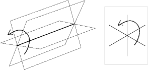
Figure 1: Product of morphisms around a stratum of codimension 2 is the identity in the dynamical groupoid. In the fundamental groupoid, the imaginary parts of the paths have to lie in one of the cones.

3.2.3

For future use, we note a generalization of $\pi_{1}(U)$ called the dynamical groupoid of the arrangement. It has the same objects and for every wall $w$ between two alcoves a single invertible matrix $B_{w}(f_{i}(z))$ which depends on the variables $z\in\mathbb{C}^{n}$ through the equation $f_{i}$ of hyperplane $H_{i}$ containing $w$. The variables $z$ are called the dynamical variables.

These matrices are required to satisfy one braid relation as in Figure 1 for any stratum of codimension 2. In other words, for the dynamical groupoid, there is a bijection

$$\begin{matrix}\textup{objects}&\leftrightarrow&\textup{$\operatorname{codim}=0$ strata}\\ \textup{morphisms}&\leftrightarrow&\textup{$\operatorname{codim}=1$ strata}\\ \textup{relations}&\leftrightarrow&\textup{$\operatorname{codim}=2$ strata}\end{matrix}$$

where strata refer to the stratification of $\mathbb{R}^{n}$. To go from the dynamical groupoid to the fundamental groupoid, we set

$$B_{w}^{\uparrow\downarrow}=\lim_{x\to\pm i\infty}B_{w}(x)\,,$$ (31)

assuming this limit exists.

We will meet the dynamical groupoids in exponential form, that is, as an arrangement of codimension $1$ subtori in an algebraic torus. The fundamental groupoid is then found from the values of $B_{w}(z)$ at the fixed points of a certain toric compactification.

The Yang-Baxter equation (8) is a very prominent example of a relation in a dynamical groupoid.

3.2.4

We now consider

$$U=H^{2}(X,\mathbb{C})\setminus\,\textup{K\"{a}hler arrangement}$$

where Kähler arrangement is the affine arrangement (29) corresponding to Kähler roots $\{\alpha\}\subset H_{2}(X,\mathbb{Z})$. It is locally finite and periodic under the action of

$$\operatorname{Pic}(X)\cong H^{2}(X,\mathbb{Z})\,.$$

The fundamental groupoid $\pi_{1}(U)$ appears in two contexts, the relation between which is rather deep. These are:

• monodromy of the quantum differential equation (18),

• autoequivalences of $\operatorname{D^{b}}\operatorname{Coh}_{\mathsf{T}}X$,

where $\mathsf{T}\subset\operatorname{Aut}(X)$ is a maximal torus.

In the early days of mirror symmetry, it was conjectured by M. Kontsevich that any $X$ and $X^{\prime}$ that have a common Kähler moduli space $\mathfrak{K}$ are derived equivalent and, moreover, there is a derived equivalence for any homotopy class of paths from $X$ to $X^{\prime}$ in the regular locus of the quantum connection. This idea became more concrete with the advent of Brigeland’s theory of stability conditions [25, 26]

More recently, it was conjectured by R. Bezrukavnikov (with perhaps some infinitesimal input from the author of these notes, which is how is often attributed in the literature, see [3, 37]) that, first, this works fully equivariantly and, second, matches specific derived automorphisms of $X$ obtained via quantization in characteristic $p\gg 0$.

3.2.5

It is clear from definitions that the groupoid $\pi_{1}(U)$ acts by monodromy, that is, analytic continuation of solutions of (18). Indeed, the natural isomorphism

$$H^{2}(X,\mathbb{C})/H^{2}(X,\mathbb{Z})\cong\operatorname{Spec}\mathbb{Z}H_{2}(X,\mathbb{Z})\subset\mathfrak{K}$$ (32)

takes $U$ to the regular locus of the quantum connection. Here $\mathbb{Z}H_{2}(X,\mathbb{Z})$ is the group algebra of the lattice $H_{2}(X,\mathbb{Z})$.

Let $z=0_{X}$ be the origin in the chart $\operatorname{Spec}\mathbb{Z}H_{2}(X,\mathbb{Z})_{\textup{eff}}$. Via the monodromy of (18), the fundamental group of $U/\operatorname{Pic}(X)$ acts on the fiber at $0$. This fiber is ${H}^{\raisebox{1.42262pt}{$\scriptscriptstyle\bullet$}}_{\mathsf{T}}(X,\mathbb{C})$, but we identify it with $K_{\mathsf{T}}(X)\otimes\mathbb{C}$ as in the work of Iritani [59]. Namely, one considers the map

$$K_{\mathsf{T}}(X)\owns\mathscr{F}\to\boldsymbol{\Gamma}\cup(2\pi i)^{\frac{\deg(\,\cdot\,)-\dim_{\mathbb{C}}X}{2}}\operatorname{ch}\mathscr{F}\in{H}^{\raisebox{1.42262pt}{$\scriptscriptstyle\bullet$}}_{\mathsf{T}}(X,\mathbb{C})_{\textup{mero}}$$ (33)

where

$$\boldsymbol{\Gamma}=\prod_{\textup{ $t_{i}$=Chern roots of $TX$}}\Gamma(1+t_{i})\,,$$

$\deg(\,\cdot\,)$ denotes the degree operator, and ${H}^{\raisebox{1.42262pt}{$\scriptscriptstyle\bullet$}}_{\mathsf{T}}(X,\mathbb{C})_{\textup{mero}}$ denotes meromorphic functions on the spectrum of ${H}^{\raisebox{1.42262pt}{$\scriptscriptstyle\bullet$}}_{\mathsf{T}}(X,\mathbb{C})$. Because of the identity

$$\Gamma(1+t)\,\Gamma(1-t)=\frac{2\pi it}{e^{\pi it}-e^{-\pi it}}\,,$$

the map (33) is an analog of Mukai’s map $\mathscr{F}\to\operatorname{ch}(\mathscr{F})\sqrt{\textup{Td}X}$ in that it is, up to a scalar multiple, an isometry for the natural sesquilinear inner products in the source and the target. It makes the monodromy act by unitary transformations of $K_{\mathsf{T}}(X)\otimes\mathbb{C}$. Iritani’s motivation was to find an integral structure in the quantum connection, and this will match nicely with what follows.

We note that the $q$-analog of the $\Gamma$-function is the function

$$\Gamma_{q}(t) =\prod_{n\geq 0}\frac{1}{1-q^{n}t}$$

$$=\operatorname{tr}\,\mathbb{C}[\textup{Maps}(\mathbb{C}(q)\to\mathbb{C}(t^{-1}))]$$ (34)

which is clearly relevant in enumerative K-theory of maps to $X$ because of the second line in (34). Here the equivariant weight of the source $\mathbb{C}(q)$ and of the target $\mathbb{C}(t^{-1})$ are indicated in parentheses. See Section 8 of [90] for how these functions come up in the quantum difference equation for $X$.

3.2.6

Quantization of equivariant symplectic resolutions is a very fertile ground which is currently being explored by several teams of researchers, see for example [3, 6, 10, 11, 12, 13, 14, 15, 19, 21, 63, 70, 71, 72, 78].

A quantization of $X$ is, first, a sheaf $\mathscr{O}_{\widehat{X}}$ of noncommutative algebras deforming the sheaf $(\mathscr{O}_{X},\{\,\cdot\,,\,\cdot\,\})$ of Poisson algebras and, second, the algebra

$$\mathscr{X}=\Gamma\left(\mathscr{O}_{\widehat{X}}\right)$$

of its global sections. In this way, very nontrivial algebras can be constructed as global section of sheaves of very standard algebras — a modern day replacement of the old dream of Gelfand and Kirillov [47]. Whenever $\mathscr{X}$ is of finite homological dimension, one has a similar global description of $\operatorname{D^{b}}\mathscr{X}\textup{-mod}$.

Quantizations $\mathscr{X}_{\lambda}$ come in families parametrized by the same data

$$\lambda\in\operatorname{Pic}(X)\otimes\textup{ground field}$$

as the commutative deformations. For Nakajima varieties, these can be described explicitly as so-called quantum Hamiltonian reductions [38].

3.2.7

While these notes are certainly not the place to survey the many successes of quantization of symplectic resolutions, certain important features of quantizations in characteristic $p\gg 0$, developed by Bezrukavnikov and Kaledin, are directly related to our narrative.

For an integral quantization parameter $\lambda$ away from certain walls, that is for

$$\lambda\in\operatorname{Pic}(X)\cap pU^{\prime}$$

where

$$U^{\prime}=\operatorname{Pic}(X)\otimes\mathbb{R}\,\setminus\,\,\textup{neighborhood of a periodic hyperplane arrangement}\,,$$

the theory produces an equivalence

$$\operatorname{D^{b}}\operatorname{Coh}_{\mathsf{A}^{(1)},\textup{supp}}X^{(1)}\xleftrightarrow{\quad\sim\quad}\operatorname{D^{b}}\mathscr{X}_{\lambda}\textup{-mod}_{\mathsf{A},\textup{supp}}$$ (35)

where

$$\mathsf{A}\subset\operatorname{Aut}(X,\omega)=\operatorname{Aut}(\mathscr{O}_{\widehat{X}_{\lambda}})$$

is a maximal torus, $X^{(1)}$ denotes Frobenius twist, and one needs to impose a certain condition on the supports of sheaves and modules in (35). We will assume that the projection of the set-theoretic support to the affinization $X_{0}$ is contracted to $0\in X_{0}$ by a certain $1$-parameter subgroup in $\mathsf{A}$; this means a version of the category $\mathscr{O}$ on the quantization side.

On the commutative side, we have a larger torus $\mathsf{T}\supset\mathsf{A}$ of automorphisms, thus the quantization side gets an extra grading so that (35) is promoted to a $\mathsf{T}$-equivariant statement. The extra grading on $\mathscr{X}_{\lambda}\textup{-mod}$ captures quite subtle representation-theoretic information. In fact, such graded lifts of representation categories are absolutely central to a lot of progress in modern representation theory, see e.g. [9, 102].

3.2.8

The map (32) send $U^{\prime}\subset\operatorname{Pic}(X)\otimes\mathbb{R}$ to the central torus $|z|=1$ in $\mathfrak{K}$ and one can associate the equivalence (35) to a straight path from the point $z=0_{X}\in\mathfrak{K}$ to a component of $U^{\prime}$.

One, meaning Bezrukavnikov, conjectures that:

1. the hyperplane arrangement in the definition of $U^{\prime}$ is the affine Kähler arrangement as in Section 3.2.4,

2. the equivalences (35) define a representation of $\pi_{1}(U)$, and

3. their action on $K_{\mathsf{T}}(X)$ equals the monodromy of the quantum differential equation,

where we use Iritani’s map as in Section 3.2.5 to lift monodromy to K-theory.

The second part of this conjecture means the following. For $\lambda\in pU^{\prime}$, the algebras $\mathscr{X}_{\lambda}$ are canonically identified for all flops of $X$ and, for two quantization parameters $\lambda,\lambda^{\prime}$ separated by a wall $w$, we can consider the induced equivalence, that is, the horizontal row in the following diagram:

(36)

The corresponding paths fall into two homotopy classes, according to the equation of the wall being effective or minus effective in $X$. Therefore, one expects all $X$ in the same class to induces the same equivalence $B_{w}^{\uparrow}$, resp. $B_{w}^{\downarrow}$, in the diagram (36). For recent results in this direction, see [18].

Note that shifts $\lambda$ by the lattice $p\operatorname{Pic}(X)$ amount to twists of $\operatorname{D^{b}}\operatorname{Coh}X^{(1)}$ by a line bundle. This gives very interesting factorizations of twists by line bundles in the group $\operatorname{Aut}\operatorname{D^{b}}\operatorname{Coh}X$.

3.2.9

For representation theory of $\mathscr{X}$, the monodromy group plays the role of Hecke algebra in the classical Kazhdan-Lusztig theory. It packages very valuable representation-theoretic information, which e.g. includes the classification of irreducible $\mathscr{X}$-modules according to their size. The latter problem inspired further conjectures by Etingof [37], which were proven in many important cases [15, 70, 100]. The general statement about monodromy is currently known [16] for Nakajima varieties $X$ such that $\dim X^{\mathsf{A}}=0$.

As we will see, the monodromy of the quantum differential equation (18) lies somewhere between the differential equation itself and its $q$-difference analog. Possible categorical interpretations of the quantum $q$-difference equations will be discussed below.

4 Stable envelopes and quantum groups

4.1 Stable envelopes

4.1.1

Let $X(\mathsf{w})$ be a Nakajima variety as in (9). Our goal in this section is to produce interesting correspondences in $X(\mathsf{w})\times X(\mathsf{w})$ which will result in actions of quantum groups and will be used to describe solutions to enumerative problems.

Note that $X(\mathsf{w})$ is disconnected, and so a correspondence in it is really a collection of correspondences in $X(\mathsf{w},\mathsf{v})\times X(\mathsf{w},\mathsf{v}^{\prime})$. Even if one is interested in correspondences in $X\times X$ for a given symplectic resolution $X$, it proves beneficial to use correspondences $X\times X^{\prime}$ as ingredients in the construction. In fact, perhaps the main obstacle in generalizing what is known for Nakajima varieties to general symplectic resolutions $X$ is the shortage of natural relatives $\{X^{\prime},X^{\prime\prime},\dots\}$ with which $X$ could meaningfully interact.

A rare general construction that one can use is the following. Let

$$\mathsf{A}\subset\operatorname{Aut}(X,\omega)$$

be a torus, not necessarily maximal. Then a choice of a $1$-parameter subgroup $\sigma:\mathbb{C}^{\times}\to\mathsf{A}$ determines a Lagrangian submanifold

$$\operatorname{Attr}=\left\{(x,y),\,\lim_{t\to 0}\sigma(t)\cdot x=y\right\}\subset X\times X^{\mathsf{A}}\,.$$ (37)

This is a very familiar concept, examples of which include e.g. conormals to Schubert cells in $T^{*}G/P$ or the loci of extensions in the moduli of framed sheaves.

The choice of $\sigma$ matters only up to the cone $\mathfrak{C}$

$$d\sigma\in\mathfrak{C}\subset\operatorname{Lie}\mathsf{A}$$

cut out by the equivariant roots of $X$ and containing $d\sigma$. We already saw these cones in Section 3.1.3. We will write $\operatorname{Attr}_{\mathfrak{C}}$ when we need to stress this dependence.

4.1.2

The submanifold $\operatorname{Attr}$ cannot be used for our purposes for the simple reason of not being closed. Using it closure, and especially the structure sheaf of the closure, runs into all the usual problems with closure in algebraic geometry. These include $\overline{\operatorname{Attr}}$ not being stable against perturbations, that is, not fitting into a family for $\mathsf{A}$-equivariant deformations $X_{\lambda}$ of $X$.

For generic $\lambda\in H^{2}(X,\mathbb{C})$, the deformation $X_{\lambda}$ is affine and (37) is closed for it. In cohomology, one gets good results by closing this cycle in the whole family, see Section 3.7 in [75]. In the central fiber $X$, this gives a Lagrangian cycle

$$\operatorname{Stab}_{\mathfrak{C}}\subset X\times X^{\mathsf{A}}\,,$$

called stable envelope, supported on the full attracting set $\operatorname{Attr}^{f}$. By definition $(x,y)\in\operatorname{Attr}^{f}$ if $x$ can be joined to $y$ by a chain of closures of attracting $\mathsf{A}$-orbits. With hindsight, one can recognize instances of this construction in such classical works as [48].

In practice, it is much more useful to have a characterization of $\operatorname{Stab}_{\mathfrak{C}}$ in terms that refer to $X$ alone instead of perturbations and closures. This becomes crucial in $\mathsf{T}$-equivariant K-theory, where $\mathsf{T}\supset\mathsf{A}$ is a torus which scales $\omega$ nontrivially. Since there are no $\mathsf{T}$-equivariant deformations of $X$, a perturbation argument does not yield a well-defined $\mathsf{T}$-equivariant K-class. In fact, as we will see, stable envelopes in K-theory crucially depend on certain data other than just a choice of a cone $\mathfrak{C}$.

4.1.3

The fixed locus has many connected components $X^{\mathsf{A}}=\bigsqcup F_{i}$ and, by definition,

$$\left(\operatorname{supp}\operatorname{Attr}^{f}_{\mathfrak{C}}\right)^{\mathsf{A}}=\bigsqcup_{i\geq j}F_{i}\times F_{j}\,,$$

where $i\geq j$ refers to the partial order on components of $X^{\mathsf{A}}$ determined by the relation of being attracted by $\sigma$. The main idea in definition of stable envelopes both in cohomology and $K$-theory is to require that

$$\operatorname{Stab}\Big{|}_{F_{i}\times F_{j}}\quad\textup{is smaller than}\quad\operatorname{Stab}\Big{|}_{F_{i}\times F_{i}}\,,$$ (38)

for $i>j$ in a sense that will be made precise presently.

The torus $\mathsf{A}$ doesn’t act on the fixed locus, so the restriction in (38) in a polynomial in equivariant variables with values in ${H}^{\raisebox{1.42262pt}{$\scriptscriptstyle\bullet$}}_{\mathsf{T}/\mathsf{A}}(F_{i}\times F_{j})$ and $K_{\mathsf{T}/\mathsf{A}}(F_{i}\times F_{j})$, respectively. We denote $\deg_{\mathsf{A}}$ the degree of this polynomial, defined as follows. In cohomology, we have a polynomial on $\operatorname{Lie}\mathsf{A}$, with the usual notion of degree. We require

$$\deg_{\mathsf{A}}\operatorname{Stab}\Big{|}_{F_{i}\times F_{j}}\quad<\quad\deg_{\mathsf{A}}\operatorname{Stab}\Big{|}_{F_{i}\times F_{i}}=\frac{1}{2}\operatorname{codim}F_{i}\,,$$ (39)

and a simple argument, see Section 3 in [75], shows that an $\mathsf{A}$-invariant cycle $\operatorname{Stab}_{\mathfrak{C}}$ supported on $\operatorname{Attr}^{f}$, equal to $\operatorname{Attr}$ near diagonal, and satisfying the degree bound (39)

1. is always unique;

2. exists for rather general algebraic symplectic varieties $X$, in particular, for all symplectic resolutions;

3. for symplectic resolutions, may be obtained by a specialization argument from Section 4.1.2.

It can be constructed inductively by a version of Gram-Schmidt process, the left-hand side in (38) is then interpreted as the remainder of division by the right-hand side. Since we are dealing with multivariate polynomials, this is somewhat nontrivial. The key observation here is that for $\mathsf{A}\subset Sp(2n)$, the class of any $\mathsf{A}$-invariant Lagrangian $L\subset\mathbb{C}^{2n}$ in $H^{2n}_{\mathsf{A}}(\mathbb{C}^{2n})$ is a $\mathbb{Z}$-multiple of the class of any fixed linear Lagrangian. A naive argument like this doesn’t work in $K_{\mathsf{A}}(\mathbb{C}^{2n})$ and things become more constrained there.

4.1.4

In K-theory, we deal with polynomials on $\mathsf{A}$ itself, for which the right notion of degree is given by the Newton polygon

$$\deg_{\mathsf{A}}\sum c_{\mu}a^{\mu}=\textup{Convex hull}\left(\{\mu,\,c_{\mu}\neq 0\}\right)\subset\mathsf{A}^{\wedge}\otimes_{\mathbb{Z}}\mathbb{R}$$

considered up to translation. The natural ordering on Newton polygons is that by inclusion and to allow for the up-to-translation ambiguity we require stable envelopes in K-theory to satisfy the condition

$$\deg_{\mathsf{A}}\operatorname{Stab}\Big{|}_{F_{i}\times F_{j}}\quad\subset\quad\deg_{\mathsf{A}}\operatorname{Stab}\Big{|}_{F_{i}\times F_{i}}+\textup{shift}_{ij}$$ (40)

for a certain collection of shifts

$$\textup{shift}_{ij}\in\mathsf{A}^{\wedge}\otimes_{\mathbb{Z}}\mathbb{R}\,.$$

Condition (40) is known as the window condition. The uniqueness of K-classes satisfying it is, again, immediate. However, existence, in general, is not guaranteed. If the rank of $\mathsf{A}$ is one, one can argue inductively using the usual division with remainder. However, for application we have in mind it is crucial to allow for tori of rank $>1$, and for them existence can only be shown for special shifts associated to fractional line bundles on $X$.

Let $\mathscr{L}\in\operatorname{Pic}_{\mathsf{A}}(X)\otimes_{\mathbb{Z}}\mathbb{R}$ be a fractional $\mathsf{A}$-linearized line bundle. Its restriction $\mathscr{L}\Big{|}_{F_{i}}$ to a component of the fixed locus has a well-defined weight in $\mathsf{A}^{\wedge}\otimes_{\mathbb{Z}}\mathbb{R}$ and we define

$$\textup{shift}_{ij}=\textup{weight}\,\mathscr{L}\Big{|}_{F_{i}}-\textup{weight}\,\mathscr{L}\Big{|}_{F_{j}}\,.$$

Note that the choice of linearization cancels out and the shift depends on just a fractional line bundle $\mathscr{L}\in\operatorname{Pic}(X)\otimes_{\mathbb{Z}}\mathbb{R}$, called the slope of the stable envelope.

There is some fine print in the correct normalization of K-theoretic stable envelopes at the diagonal. It involves the notion of a polarization, see [90] for details. In fact, even in cohomology, it is best to require $\operatorname{Stab}=\pm\operatorname{Attr}$ near the diagonal, depending on a polarization, see [75]. With such normalization and for a certain class of $X$ that includes all symplectic resolutions, we have

Theorem 1 ([76, 1, 55]).

There exists unique stable envelope

$$\operatorname{Stab}_{\mathfrak{C},\mathscr{L}}\in K_{\mathsf{T}}(X\times X^{\mathsf{A}})$$ (41)

for any cone $\mathfrak{C}$ and any slope $\mathscr{L}$ away from a certain locally finite $\operatorname{Pic}(X)$-periodic rational hyperplane arrangement in $\operatorname{Pic}(X)\otimes_{\mathbb{Z}}\mathbb{R}$.

Proofs in the literature deduce this from more general statements. For Nakajima varieties, the existence of more general elliptic stable envelopes is shown in [1] , see Section 3.8 there for specialization to K-theory. The paper [55] gives a Gram-Schmidt-style existence proof of categorical stable envelopes.

Note that for generic shifts, the inclusion in (40) is necessarily strict as the inclusion of an integral polytope into a very nonintegral one. Therefore, the $\mathscr{L}$-dependence of $\operatorname{Stab}_{\mathfrak{C},\mathscr{L}}$ is locally constant and can only jump if a lattice point gets on the boundary of the polytope on the right in (40).

There is a direct relation between stable envelopes and the monodromy of (18) proven in [1] in the more general $q$-difference case. It implies, in particular that

$$\left\{\begin{matrix}\textup{hyperplanes in $\operatorname{Pic}(X)\otimes_{\mathbb{Z}}\mathbb{R}$ }\\ \textup{where $\operatorname{Stab}_{\mathfrak{C},\mathscr{L}}$ jump}\end{matrix}\right\}\,{\Huge\subset}\,\left\{\begin{matrix}\textup{K\"{a}hler arrangement}\\ \textup{for $X$}\end{matrix}\right\}\,,$$ (42)

and I think that we have an equality in (42) aside from trivialities like $X=X_{1}\times X_{2}$ with $\mathsf{A}$ acting on $X_{2}$ only. Also note that the left-hand side in (42) does not depend on $\mathfrak{C}$.

4.1.5

Piecewise constant dependence on a fractional line bundle should certainly activate neurons in areas of the cerebral cortex responsible for multiplier ideal sheaves and related objects. Indeed, the similarity goes further in that

1. window conditions are preserved by proper push-forwards;

2. in a normal-crossing situation (e.g. for hypertoric varieties), stable envelope is a twist of a structure sheaf by a rounding of $\mathscr{L}$.

In particular, Nakajima varieties are related by certain Lagrangian abelianization correspondences to smooth hypertoric varieties, see [56], and this has been used to compute stable envelopes starting in [101, 98] and all the way to the elliptic level of generality in [1].

4.1.6

Favorable properties of stable envelopes are shared by their categorical lifts, which are defined as functors

$$\mathbf{Stab}_{\mathfrak{C},\mathscr{L}}:\operatorname{D^{b}}\operatorname{Coh}_{\mathsf{T}}X^{\mathsf{A}}\to\operatorname{D^{b}}\operatorname{Coh}_{\mathsf{T}}X$$ (43)

satisfying the same window conditions for the derived restriction to $X^{\mathsf{A}}$. For $\operatorname{rk}\mathsf{A}=1$, a detailed study of these, with many applications, can be found the in the work of Halpern-Leistner [54], see also [5]. In this case, one doesn’t need the shift to come from a line bundle. The case of tori of higher rank is considered in [55].

4.2 R-matrices

4.2.1

If a construction in algebraic geometry requires additional choices, such as the choice of a cone $\mathfrak{C}$ and a slope $\mathscr{L}$ in the definition of stable envelopes, then this can be viewed as a liability or as an asset. The latter point of view is gaining popularity as people find more and more applications of wall-crossing phenomena of various kind. In the case at hand, it will be beneficial to study how stable envelopes change as the we cross the wall from $\mathfrak{C}$ to another chamber $\mathfrak{C}^{\prime}\subset\operatorname{Lie}\mathsf{A}$, or as we cross a wall of the Kähler arrangement from $\mathscr{L}$ to $\mathscr{L}^{\prime}$.

To formalize this, we introduce

$$R^{\mathscr{L}}_{\mathfrak{C}^{\prime}\leftarrow\mathfrak{C}}=\operatorname{Stab}_{\mathfrak{C}^{\prime},\mathscr{L}}^{-1}\,\circ\,\operatorname{Stab}_{\mathfrak{C},\mathscr{L}}$$ (44)

and similarly

$$R^{\mathfrak{C}}_{\mathscr{L}^{\prime}\leftarrow\mathscr{L}}=\operatorname{Stab}_{\mathfrak{C},\mathscr{L}^{\prime}}^{-1}\,\circ\,\operatorname{Stab}_{\mathfrak{C},\mathscr{L}}\,.$$ (45)

Stable envelopes are isomorphisms after localization, so

$$\textup{all $R$-matrices}\subset\operatorname{End}(K_{\mathsf{T}}(X^{\mathsf{A}}))\otimes\mathbb{Q}(\mathsf{T})\,.$$

They depend on equivariant variables $a\in\mathsf{A}$ for the torus $\mathsf{A}$ which does not act on $X^{\mathsf{A}}$, and this is, again, a bonus. We can expand R-matrices as $a\to 0$, where $0$ is a fixed points of a toric compactification $\overline{\mathsf{A}}\supset\mathsf{A}$ that correspond to the fan $\{\mathfrak{C}_{i}\}$ of chambers. The coefficients of this expansion give countably many operators acting on integral $\mathsf{T}/\mathsf{A}$-equivariant K-theory of $X^{\mathsf{A}}$, that is, we can view $R$-matrices as interesting generating functions for correspondences in $X^{\mathsf{A}}$.

4.2.2

Let $\mathfrak{C}$ and $\mathfrak{C}^{\prime}$ be separated by a wall in $\operatorname{Lie}\mathsf{A}$. This wall is of the form $\operatorname{Lie}\mathsf{A}^{\prime}$ for some codimension 1 subtorus $\mathsf{A}^{\prime}\subset\mathsf{A}$. One shows, see Section 9.2 in [90] that

$$R_{\mathfrak{C}^{\prime}\leftarrow\mathfrak{C}}\textup{ for $\mathsf{A}$-action on $X$ }=\,R_{\mathfrak{C}^{\prime}\leftarrow\mathfrak{C}}\textup{ for $\mathsf{A}/\mathsf{A}^{\prime}$-action on $X^{\mathsf{A}^{\prime}}$ }$$ (46)

and, in particular, $R_{\mathfrak{C}^{\prime}\leftarrow\mathfrak{C}}$ factors through the map $\mathsf{A}\to\mathsf{A}/\mathsf{A}^{\prime}$, that is, through the equation of the wall. This gives

Proposition 4.1.

Matrices $R_{\mathfrak{C}^{\prime}\leftarrow\mathfrak{C}}$ form a representation of the dynamical groupoid for the central arrangement defined by the equivariant roots of $X$.

Here central is used as opposite of affine: we equate equivariant roots to $0$ and not to an arbitrary integer.

4.2.3

In the situation of Section 2.2.5, the root hyperplane are $a_{i}/a_{j}=1$ and the groupoid relation becomes the Yang-Baxter equation.

This geometric solution of the YB equation produces a geometric action of a quantum group $\mathscr{A}=\mathscr{U}_{\hbar}(\widehat{\mathfrak{g}})$ for a certain Lie algebra $\mathfrak{g}$ as indicated in Section 1.12 . See [75, 92] for the details of the reconstruction.

The parallel procedure in cohomology constructs a certain degeneration $\mathsf{Y}(\mathfrak{g})$ of $\mathscr{U}_{\hbar}(\widehat{\mathfrak{g}})$ known as the Yangian of $\mathfrak{g}$. This is a Hopf algebra deformation of $\mathscr{U}(g[t])$ and the universal enveloping of $\mathfrak{g}\subset\mathfrak{g}[t]$

$$\mathscr{U}(\mathfrak{g})\subset\mathsf{Y}(\mathfrak{g})$$ (47)

remains undeformed as a Hopf algebra.

4.2.4

The structure of $\mathscr{A}$ may be analyzed using the following useful connection between R-matrices of the two kinds (44) and (45).

We can include $\mathscr{L}$ into an infinite sequence of slopes

$$\dots,\mathscr{L}_{-2},\mathscr{L}_{-1},\mathscr{L}_{0}=\mathscr{L},\mathscr{L}_{1},\mathscr{L}_{2},\dots$$ (48)

that go from a point $\mathscr{L}_{-\infty}$ on the minus ample infinity of $\operatorname{Pic}(X)$ to a point $\mathscr{L}_{\infty}$ on the ample infinity of $\operatorname{Pic}(X)$. A choice of such path is analogous to a choice of the factorization of the longest element in Weyl group in the usual theory.

Tautologically,

$$R^{\mathscr{L}}_{(-\mathfrak{C})\leftarrow\mathfrak{C}}=\overrightarrow{\prod_{i<0}}R^{-\mathfrak{C}}_{\mathscr{L}_{i+1}\leftarrow\mathscr{L}_{i}}\,\,R_{(-\mathfrak{C},\mathscr{L}_{-\infty})\leftarrow(\mathfrak{C},\mathscr{L}_{\infty})}\,\,\overleftarrow{\prod_{i\geq 0}}R^{\mathfrak{C}}_{\mathscr{L}_{i+1}\leftarrow\mathscr{L}_{i}}\,,$$ (49)

assuming the term in the middle makes sense, that is, infinite product converge in a suitable topology. This is indeed the case:

Proposition 4.2 ([92]).

The operator $R_{(-\mathfrak{C},\mathscr{L}_{-\infty})\leftarrow(\mathfrak{C},\mathscr{L}_{\infty})}$ is well-defined and acts by an operator of multiplication in $K_{\mathsf{T}}(X^{\mathsf{A}})$.

In fact, this operator acts by a very specific Schur functor of the normal bundle $N_{X/X^{\mathsf{A}}}$ to the fixed locus.

Formula (49) generalizes factorization of R-matrices constructed in the conventional theory of quantum groups, see for example [65, 66, 67].

Recall that $\mathscr{U}_{\hbar}(\widehat{\mathfrak{g}})$ is spanned by coefficients in $u\in\mathsf{A}\cong\mathbb{C}^{\times}$ of the matrix coefficients of R-matrices (44). In this procedure, one can, in fact, pick out the matrix coefficients of each individual term in the factorization (49) and this gives

$$\mathscr{U}_{\hbar}(\mathfrak{g}_{w})\hookrightarrow\mathscr{U}_{\hbar}(\widehat{\mathfrak{g}})$$ (50)

for each wall $w$ crossed by the path (48). These deform the decomposition

$$\widehat{\mathfrak{g}}=\mathfrak{g}[t^{\pm 1}]=\widehat{\mathfrak{h}}\oplus\bigoplus_{w}\mathfrak{g}_{w}\,,\quad\mathfrak{g}_{w}=\bigoplus_{\textup{$\alpha=-n$ on $w$}}\mathfrak{g}_{\alpha}t^{n}\,,$$ (51)

in which the $\widehat{\mathfrak{h}}$ part corresponds to the middle factor in (49). Note that the subalgebra (50) depends on

1. the wall $w$ between two alcoves and not only on the hyperplane containing it and, moreover, on

2. the choice of the path (48).

These features are already familiar from the classical theory of quantum groups. Concretely, in textbooks, quantum groups are usually presented by generators and relations and, consequently, come equipped with root subalgebras corresponding to simple roots. Constructing other root subalgebras requires choices just like we had to make in (48).

This argument also shows that the quantum group constructed using the R-matrix (49) is independent of the choice of $\mathscr{L}$.

4.3 Enumerative operators

4.3.1

We go back to curve-counting in cohomology and reexamine the operator (17) for Nakajima varieties. Recall the inclusion (47). The root decomposition in (25) is according to the components of $X(\mathsf{w})$, that is,

$$\mathfrak{g}_{\alpha}:{H}^{\raisebox{1.42262pt}{$\scriptscriptstyle\bullet$}}(X(\mathsf{v},\mathsf{w}))\to{H}^{\raisebox{1.42262pt}{$\scriptscriptstyle\bullet$}}(X(\mathsf{v}-\alpha,\mathsf{w}))\,,$$ (52)

and all these root spaces are finite-dimensional. In parallel to Kac-Moody theory, one shows that all roots are either positive or negative, that is,

$$\textup{roots of $\mathfrak{g}$}\subset\mathbb{N}^{I}\cup(-\mathbb{N})^{I}\,.$$

Duality (26) gives a canonical element

$$\operatorname{Casimir}_{\alpha}\in\,:\!\mathfrak{g}_{-\alpha}\mathfrak{g}_{\alpha}\!:\,\subset\mathscr{U}(\mathfrak{g})$$

which preserves ${H}^{\raisebox{1.42262pt}{$\scriptscriptstyle\bullet$}}X(\mathsf{v},\mathsf{w})$ and annihilates it unless $|\alpha|\leq\mathsf{v}$ because of (52). Normal ordering here means that we act by lowering operators first.

The main result of [75] is the following

Theorem 2.

For Nakajima quiver varieties, formula (20) holds with

$$L_{\alpha}=-\operatorname{Casimir}_{\alpha}\,.$$

In particular, this gives a new computations of the quantum cohomology of Hilbert schemes of ADE surfaces, first obtained in [91, 74] by a more direct analysis.

4.3.2

The proof of Theorem 2 given in [75] is rather indirect. Recall that the group $\prod GL(W_{i})$ in (15) acts on $X(\mathsf{v},\mathsf{w})$, and this action is nontrivial if $\sum\mathsf{w}_{i}>1$. There is a flat difference connection in the corresponding equivariant variables which commutes with the quantum connection (18). It is constructed geometrically counting sections in certain twisted $X$-bundles over $\mathbb{P}^{1}$. Operators of this kind, often called shift operators, find many other applications in enumerative geometry, see for example [60].

The main step of the proof identifies this commuting connection with what is known as the quantum Knizhnik-Zamolodchikov equations. These were introduced by Frenkel and Reshetikhin in [46] in the context of quantum loop algebras of finite-dimensional Lie algebras. They make sense for any solution of the Yang-Baxter equation with a spectral parameter and, in particular, for our geometrically constructed R-matrices. The support and the degree conditions satisfied by stable envelopes enter the argument at this step.

The K-theoretic computation in [90, 92], while much more involved on the technical level, follows the same general strategy: one identifies a commuting difference connection first, and uses that to constrain the connection of principal geometric interest.

4.3.3

One may phrase the answer in Theorem 2 as the identification of the quantum connection (18) with the trigonometric Casimir connection for the Yangian $\mathsf{Y}(\mathfrak{g})$. For finite-dimensional Lie algebras, such connections were studied by Toledano Laredo in [107], see also the work [105, 106] by Tarasov and Varchenko.

A connection with Yangians was expected from the ideas of Nekrasov and Shatashvili. The precise identification with the Casimir connection was suggested by Bezrukavnikov, Etingof, and their collaborators. Back then, it was further predicted by Etingof that the correct K-theoretic version of the quantum connection should be a generalization of the dynamical Weyl group studied by Tarasov, Varchenko, Etingof, and others for finite-dimensional Lie algebras $\mathfrak{g}$, see e.g. [104, 41]. Indeed, for such $\mathfrak{g}$, Balagovic showed [4] that the dynamical $q$-difference equations degenerate to the Casimir connection in an appropriate limit.

At that moment in time, there was neither geometric, nor a representation-theoretic construction of the required $q$-difference connection.

4.3.4

Referring the reader to [31] for all details, we will define a quasimap

$$f:C\dashrightarrow X=\widetilde{X}/\!\!/G$$

to a GIT quotient as a section of a bundle of prequotients $\mathscr{P}\times_{G}X$, up to isomorphism. Here $\mathscr{P}$ is a principal $G$-bundle over $C$ which is a part of the data and is allowed to vary. Stability conditions for quasimaps are derived from stability on $\widetilde{X}$; we will use the simplest one that requires the value of the quasimap be stable at the generic point of $C$.

To have an evaluation map at a specific point $p\in C$ one introduces quasimaps relative $p$, formed by diagrams of the form

(53)

in which $\pi$ is an isomorphism over $C\setminus\,p$ and contracts a chain of rational curves joining $p^{\prime}$ to $\pi^{-1}(C\setminus\,p)$. The evaluation map records the value at $p^{\prime}$.

For quasimaps to $X(\mathsf{v},\mathsf{w})$, we have $G=\prod GL(V_{i})$ and so a principal $G$-bundle is the same as a collection of vector bundles of ranks $\mathsf{v}$. For a regular map $f$, these are the pullbacks $f^{*}\mathscr{V}_{i}$ of the tautological vector bundles $\mathscr{V}_{i}$ on $X$. We denote them by $f^{*}\mathscr{V}_{i}$ for all quasimaps; they are a part of the data of a quasimap.

Consider the line bundle

$$\mathscr{L}_{i}=\det\mathscr{V}_{i}\in\operatorname{Pic}(X)\,.$$

For our difference connection, we need a correspondence in $X$ that generalizes the operator $\otimes\mathscr{L}_{i}$ in $K_{\mathsf{T}}(X)$. We take

$$\mathbf{M}_{\mathscr{L}_{i}}=\sum_{d}z^{d}\,\operatorname{ev}_{*}\left(\widehat{\mathscr{O}}_{\mathscr{M}_{d}}\otimes\det{H}^{\raisebox{1.42262pt}{$\scriptscriptstyle\bullet$}}(f^{*}\mathscr{V}_{i}\otimes\pi^{*}\mathscr{O}_{p_{1}})\right)\,\mathbf{G}^{-1}\,,$$ (54)

where $\mathscr{M}_{d}$ is the moduli space of quasimaps

$$(\mathbb{P}^{1},0,\infty)\cong(C,p_{1},p_{2})\dasharrow\widetilde{X}/\!\!/G$$

of degree $d$ and $\mathbf{G}$ is the glue matrix from (24). See [90] for detailed discussion of how one arrives at the definition (54) and what is the geometric significance of the solutions of the corresponding $q$-difference equations.

4.3.5

On the algebraic side, recall the subalgebras (50) associated to a wall of the Kähler arrangement. It is by itself a quantum group, in particular, it has its own R-matrix $R_{w}$, which is the corresponding factor in (49) with a suitable normalization. This is not a quantum loop algebra, in fact it is a quantum group of rank 1. Correspondingly, $R_{w}$ does not have a spectral parameter and satisfies the YB equation (8) for constant (in $u$) operators. Examples of these wall subalgebras are $\mathscr{U}_{\hbar}(\mathfrak{sl}(2))$ and the quantum Heisenberg algebra.

By definition, quantum Heisenberg algebra has two group-like invertible elements

$$\Delta H=H\otimes H\,,\quad\Delta K=K\otimes K\,,$$

of which $K$ is central, while

$$HE=\hbar\,EH\,,\quad HF=\hbar^{-1}FH\,.$$

Here the generators $E$ and $F$ satisfy

$$\left[E,F\right]=\frac{K-K^{-1}}{\hbar-\hbar^{-1}}$$

and comultiply as follows

$$\Delta E =E\otimes 1+K^{-1}\otimes E\,.$$

$$\Delta F =F\otimes K+1\otimes F\,.$$

This algebra acts on $\mathbb{Z}[x,\hbar^{\pm 1}]$ by

$$E=x\,,\quad F=-\frac{d}{dx}\,,\quad H=\hbar^{x\tfrac{d}{dx}}\,,\quad K=\hbar\,.$$

Its R-matrix is

$$R=\hbar^{\Omega}\,\exp\left(-(\hbar-\hbar^{-1})F\otimes E\right)\,,$$

where

$$\Omega=-\log_{\hbar}H\otimes\log_{\hbar}H=-x\tfrac{d}{dx}\otimes x\tfrac{d}{dx}\,.$$

In its geometric origin, the $\mathbb{Z}$-valued operator $\Omega$ records the codimension of the fixed locus.

For quivers of affine type, every root is either real, in which case the wall subalgebra is isomorphic to $\mathscr{U}_{\hbar}(\mathfrak{sl}(2))$, or has zero norm. In the latter case, all multiples of the root enter $\mathfrak{g}_{w}$ in (51) and $\mathscr{U}_{\hbar}(\mathfrak{g}_{w})$ is a countable product of Heisenberg subalgebras, with their tori identified. For example, all root subalgebra of the algebra $\mathscr{U}_{\hbar}(\widehat{\widehat{\mathfrak{gl}}}(1))$ associated with the quiver with one vertex and one loop are of this type. The structure of this algebra has been studied by many authors, see for example [29, 43, 44, 85].

4.3.6

With any R-matrix, we can associate

$$\textup{qKZ operator}=(z^{\log_{\hbar}H}\otimes 1)\,R=(z^{\log_{\hbar}H}\otimes 1)\,\hbar^{\Omega}+\dots$$ (55)

acting in the tensor product of two $\mathscr{U}_{\hbar}(\mathfrak{g}_{w})$-modules. Here dots stand for an upper-triangular operator.

Since $\mathscr{U}_{\hbar}(\mathfrak{g}_{w})$ is not a loop algebra, this is not a difference operator. Instead of a fundamental solution of a difference equation, we can ask for a unipotent matrix $\mathsf{J}$ that conjugates (55) to its eigenvalues

$$(z^{\log_{\hbar}H}\otimes 1)\,R\,\mathsf{J}=\mathsf{J}\,(z^{\log_{\hbar}H}\otimes 1)\,\hbar^{\Omega}\,.$$ (56)

Such operator exist universally and for the quantum Heisenberg algebra it equals

$$\mathsf{J}=\exp\left(-(\hbar-\hbar^{-1})\frac{z}{1-z}\,F\otimes E\right)\in\mathscr{U}_{\hbar}(\mathfrak{g}_{w})^{\otimes 2}[[z]]\,.$$

It is called the fusion operator. It gives a certain canonical way to promote the R-matrix to a rational function on the maximal torus.

We have a maximal torus

$$\textup{K\"{a}hler torus}\times\mathbb{C}^{\times}_{q}\subset\operatorname{Aut}\widehat{\mathfrak{g}}$$ (57)

where

$$\textup{K\"{a}hler torus}=\operatorname{Pic}(X)\otimes\mathbb{C}^{\times}=\textup{maximal torus of $\mathfrak{g}$}\big{/}\textup{center}\,,$$

and $\mathbb{C}^{\times}_{q}$ acts naturally by automorphisms of domains of quasimaps and on $\widehat{\mathfrak{g}}$ via the loop rotation automorphism (7). The adjoint action of (57) on $\mathscr{U}_{\hbar}(\mathfrak{g}_{w})$ factors through a map to its maximal torus, so $\mathsf{J}$ can be promoted to a function on (57). Since the larger torus includes a shift by $q$, the equation (56) is trivially promoted to a $q$-difference equation.

4.3.7

From the fusion operator $\mathsf{J}$, one can make the following dynamical operator

$$\mathsf{B}_{w}=\mathsf{m}\left((1\otimes\mathsf{S}_{w})\,\mathsf{J}_{21}^{-1}\right)$$ (58)

where

$$\mathsf{m} =\textup{multiplication}\,,$$

$$\mathsf{S}_{w} =\textup{antipode of $\mathscr{U}_{\hbar}(\mathfrak{g}_{w})$}\,,$$

and $\mathsf{J}_{21}=(12)\,\mathsf{J}$.

Compare this with the operator

$$\operatorname{Casimir}_{\alpha}=\mathsf{m}\,\mathbf{r}_{\alpha}\,,\quad\mathbf{r}_{\alpha}\in\mathfrak{g}_{-\alpha}\otimes\mathfrak{g}_{\alpha}\,,$$

in which the canonical tensor $\mathbf{r}_{\alpha}$ is the $\alpha$-component of the classical R-matrix, see Section 4.8 in [75].

This is not how the dynamical Weyl group is defined in [41], but one can find a formula equivalent to (58) for $\mathfrak{g}_{w}=\mathfrak{sl}(2)$ there. The abstract formula (58) makes sense in complete generality, for any $R$-matrix.

The main result of [92] may be summarized as follows. Let $\nabla\subset H^{2}(X,\mathbb{R})$ be the Kähler alcove which coincides with the negative ample cone near zero.

Theorem 3.

The operators $\mathsf{B}_{w}$ define a representation of the dynamical groupoid of the affine Kähler arrangement. We have

$$\mathbf{M}_{\mathscr{L}}=\textup{const}\,\mathscr{L}\,\,\dots\mathsf{B}_{w_{3}}\mathsf{B}_{w_{2}}\mathsf{B}_{w_{1}}$$ (59)

where $w_{1},w_{2},\dots$ is the ordered set of wall crossed on the way from $\nabla$ to $\nabla-\mathscr{L}$, and

$$\mathbf{G}=\textup{const}\,\mathsf{B}_{w^{\prime}_{1}}\mathsf{B}_{w^{\prime}_{2}}\dots$$ (60)

where $w^{\prime}_{1},w^{\prime}_{2},\dots$ are the walls crossed on the way from $\nabla$ to $-\nabla$.

In other words, the operators $\mathbf{M}_{\mathscr{L}}$ come from the lattice part of the dynamical groupoid, while the glue matrix $\mathbf{G}$ is the dynamical analog of the longest element of the finite Weyl group.

The constant factor ambiguity in Theorem 3 is of the same nature as the diagonal ambiguity in (20).

4.3.8

The factorizations of the operators $\mathbf{M}_{\mathscr{L}}$ provided by Theorem 3 generalize the additive decomposition (20) of the operators of the quantum differential connection.

It is certainly natural to expect parallel factorizations and a dynamical groupoid action for an arbitrary symplectic resolution $X$. Note that if factorizations of the required kind exists, they are unique and determine the whole structure.

Some speculations of what this might look like will be offered below. One should bear in mind, however, that both the quasimap moduli spaces and the operators $\mathbf{M}_{\mathscr{L}}$, $\mathbf{G}$ depend on the choice of the presentation (23). This can be seen in example (28).

4.3.9

The knowledge of the quantum difference equation opens the door to the reconstruction of the K-theoretic DT theory of ADE fibrations and toric varieties in the same way as it was done in cohomology [73]. For a technical introduction to the subject, see e.g.  [90].

4.3.10

As in cohomology, one can define a flat $q$-difference connection on the space of equivariant parameters by counting twisted quasimaps to $X$. For twisted quasimaps, the spaces $W_{i}$, $Q_{ij}$ from Section 2.2.1 and their duals $\hbar^{-1}\otimes W_{i}^{\vee}$, $\hbar^{-1}\otimes Q_{i,j}^{\vee}$ form fixed but possibly nontrivial bundles over the domain $C$ of the quasimap. The $\hbar^{-1}$-weight here may also be twisted, that is, replaced by a line bundle on $C$.

On general grounds, the quantum $q$-difference connection commutes with these shift operators. A key step in in the proof Theorem 3 it to find the quantum Knizhnik-Zamolodchikov connection among the shift operators. See Section 10 of [90] for details.

If we don’t shift $\hbar$, that is, if we restrict ourselves to twisting by a maximal torus $\mathsf{A}\subset\operatorname{Aut}(X,\omega)$, then the resulting $q$-difference connection is a connection with regular singularities on the toric variety $\overline{\mathsf{A}}$ defined by the fan of cones $\{\mathfrak{C}\}\subset\operatorname{Lie}\mathsf{A}$. Dually, the quantum difference connection is a connection with regular singularities on $\mathfrak{K}$, which is a toric variety defined by the fan of ample cones. These two connections commute but are not regular jointly — this will be important below.

The two connections are conjectured to be exchanged by symplectic duality, up-to an explicit gauge transformation.

5 Further directions

5.1 Categorical dynamical groupoid

5.1.1

The operators $\mathsf{B}_{w}$ of the dynamical groupoid from Theorem 3 are normalized so that $\mathsf{B}_{w}\big{|}_{z=0}=1$ where $0=0_{X}\in\mathfrak{K}$ is the origin in the space of Kähler variables for $X$. This is natural from the curve-counting point of view. One can choose a more symmetric normalization, in which the specialization to K-theoretic Bezrukavnikov’s groupoid from Section 3.2.8 is the standard (31). In that normalization, one takes the factorization of $\mathscr{L}$ provided by Bezrukavnikov’s theory and distributes it over the factors in (59).

5.1.2

It is natural to ask for a categorical lift of the dynamical groupoid. The dependence on the Kähler variables may be treated either formally or not formally. In the formal treatment, we introduce an extra grading by the characters $H_{2}(X,\mathbb{Z})$ of the Käher torus, otherwise nothing is changed.

The functors $B_{w}$ from the triangle (36) are perverse equivalences as in the work of Rouquier and collaborators [34], see [3, 71, 72]. This means, in particular, that the category

$$\operatorname{D^{b}}\mathscr{X}_{\lambda}\textup{-mod}=\mathscr{C}\supset\mathscr{C}_{1}\supset\mathscr{C}_{2}\supset\dots\supset\mathscr{C}_{k}$$

has a finite filtration by thick subcategories such that the action of $B_{w}$ on each successive quotient $\mathscr{C}_{i}/\mathscr{C}_{i+1}$ is a shift of homological degree and equivariant grading.

From (59) and (60) it is natural to expect the dynamical lift $B_{w}(z)$ to be the glue matrix $\mathbf{G}_{\mathscr{C}_{i}/\mathscr{C}_{i+1}}$ on each successive quotient, with a shift as before. This requires a geometric realization of the quotient category $\mathbf{G}_{\mathscr{C}_{i}/\mathscr{C}_{i+1}}$. In fact, if one wants to use quasimaps to define the glue matrix as in (24), one needs a presentation

$$\mathscr{C}_{i}/\mathscr{C}_{i+1}\cong\operatorname{D^{b}}\operatorname{Coh}_{\begin{subarray}{c}\textup{reductive}\\ \textup{group}\end{subarray}}\begin{pmatrix}\textup{lci affine}\\ \textup{prequotient}\end{pmatrix}\bigg{/}\textup{unstable}\,.$$

Perhaps such presentation for each possible quotient may be obtained from a GIT presentation (23) for $X$ itself. Perhaps there are ways to define the curve-counting operators which are more general than those based on quasimap spaces. In any case, it will require some additional data, as our running example (28) shows.

5.2 Elliptic theory

5.2.1

The Yang-Baxter equation (8) has a generalization, in which the matrix $R(u)$ is allowed to depend on a variable $z$ in the maximal torus for the corresponding group. This is known as the dynamical Yang-Baxter equations and it has very interesting solutions in elliptic functions of $u$ and $z$. These have to do with the theory of elliptic quantum groups, which was started by Felder [45] and has since grown into a very rich subject.

As anticipated in [49] at the dawn of the subject, one gets elliptic quantum groups by lifting the constructions of the geometric representation theory to equivariant elliptic cohomology.

Elliptic stable envelopes were constructed in [1]. Their main conceptual difference with both K-theoretic and categorical stable envelopes is the following. While stable envelopes from Section 4 have a piecewise constant dependence on the slope $\mathscr{L}\in\operatorname{Pic}(X)\otimes_{Z}\mathbb{R}$, elliptic stable envelopes depend analytically on their dynamical variable

$$z\in\operatorname{Pic}(X)\otimes_{\mathbb{Z}}E\,,\quad E=\mathbb{C}^{\times}/q^{\mathbb{Z}}\,.$$

The piecewise constant dependence is recovered in the $q\to 0$ limit if

$$-\,\Re\,\frac{\ln z}{\ln q}\to\mathscr{L}\,.$$

It is, of course, well-known that elliptic functions have a piecewise analytic asymptotics as the elliptic curve degenerates.

The walls across which K-theoretic stable envelopes jump played an absolutely key role in the preceding discussion. In the elliptic theory, walls become poles and all alcoves melt into a single elliptic function. The only remaining discrete data is the choice of a cone $\mathfrak{C}\subset\operatorname{Lie}\mathsf{A}$, and the choice of the ample cone in $H^{2}(X,\mathbb{R})$ if one thinks about all flops of $X$ at the same time. Note that this data is now symmetric on the two sides of the symplectic duality.

5.2.2

A categorical lift of elliptic stable envelopes along the lines of (43) should incorporate their dependence on the Kähler variables $z$ together with the elliptic modulus $q$. A few paragraphs ago we discussed adding such extra variables formally. A real need to incorporate these variables arises in certain categories of boundary conditions, see [64] for a general introduction to the topic.

Recall that the Nakajima varieties may be interpreted as the Higgs branches of the moduli spaces of vacua in certain supersymmetric gauge theories. K-theoretic counts of quasimaps $C\dasharrow X$, where $C$ is a Riemann surface, may then be interpreted as supersymmetric indices in 3-dimensional gauge theories with spacetime $C\times S^{1}$.

A boundary condition in such theory is a coupling of the bulk gauge theory to some $(0,2)$-supersymmetric theory on $\partial C\times S^{1}$. The Hilbert space of the boundary theory is graded by

$$\textup{K\"{a}hler torus of $X$}=\textup{Center of the gauge group}$$

together with the action of $q$ by rotations of $\partial C$. These Hilbert spaces form a sheaf over $X$ and taking their graded index one gets an element of $K_{\mathsf{T}}(X)(z)[[q]]$ which represents the $q$-expansion of an elliptic function. This is how elliptic stable envelopes should appear from a functor

$$\begin{matrix}\textup{boundary condition}\\ \textup{in gauge theory for $X^{\mathsf{A}}$}\end{matrix}\quad\xrightarrow{\quad}\quad\begin{matrix}\textup{boundary condition}\\ \textup{in gauge theory for $X$}\end{matrix}\quad,$$ (61)

as will be discussed in [2].

Note that elliptic stable envelopes depend only on $X$ itself and not on its presentation as a Nakajima variety.

5.2.3

While the monodromy of a differential equation gives a representation of the fundamental group of its regular locus, the monodromy of a $q$-difference equation in $z$ is a collection of elliptic matrices in $z$ that relate different fundamental solutions. In particular, $q$-connections with regular singularities on a toric variety produce elliptic connection matrices for any pair of fixed points. For us, those are labeled by a pair of birational symplectic resolutions $X$ for the Kähler $q$-connection or by a pair of cones in $\operatorname{Lie}\mathsf{A}$ for the equivariant $q$-connection.

This difference in how monodromy packages the information is parallel to the differences highlighted in Section 5.2.1 and, in fact, elliptic stable envelopes give a very powerful tool for the analysis of the monodromy.

5.2.4

Recall from Section 4.3.10 that the Kähler and equivariant connections are regular separately but not jointly. This can never happen for differential equations by a deep result of Deligne [36], but can happen very easily for $q$-difference equations as illustrated by the following system:

$$f(qz,a)=af(z,a)\,,\quad f(z,qa)=zf(z,a)\,.$$

This proves to be a feature and not a bug, for the following reason.

Let $0_{X}\in\mathfrak{K}$ be the origin in the Kähler moduli space for $X$ and choose a point $0_{\mathsf{A}}\in\overline{\mathsf{A}}$ on the infinity of the equivariant torus. Quasimap counting produces solutions of both Kähler and equivariant equations known as vertex functions, or I-functions in the mirror symmetry vernacular. These are born as power series in $z$, the terms in which record the contribution of quasimaps of different degrees. In particular, vertex functions are holomorphic in $z$ in a punctured neighborhood of $0_{X}$. However, they have poles in $a$ accumulating to $0_{\mathsf{A}}$.

We can call these the $z$-solutions, and there are the dual $a$-solutions that are holomorphic in a punctured neighborhood of $0_{\mathsf{A}}$. The connection matrix between the $z$-solutions and the $a$-solutions is an elliptic matrix in both $z$ and $a$. It may be called the pole subtraction matrix because it may be, in principle, computed by canceling the unwanted poles. It may be compared to a monodromy matrix, or to a Stokes matrix, except there is no analytic continuation involved, or sectors. One of the main results of [1] is the identification of pole subtraction matrices with stable envelopes. Note they depend on the same discrete data, namely a choice of $(0_{X},0_{\mathsf{A}})\in\mathfrak{K}\times\overline{A}$, and act in the direction

$$K_{\mathsf{T}}(X^{\mathsf{A}})\otimes\textup{functions}(z,a,\hbar,q)\to K_{\mathsf{T}}(X)\otimes\textup{same functions}\,.$$ (62)

K-theories in the source and the target of (62) are naturally identified with initial conditions for $a$-solutions and $z$-solutions, respectively.

5.2.5

A combination of two steps of the form

$$\begin{matrix}\textup{fundamental}\\ \textup{solution at $0_{\mathsf{A}}$}\end{matrix}\quad\xrightarrow{\quad\textup{elliptic stable envelope}\quad}\quad\begin{matrix}\textup{fundamental}\\ \textup{solution at $0_{\mathsf{X}}$}\end{matrix}$$

connect any two fixed points of $\mathfrak{K}$ or $\overline{\mathsf{A}}$. As a result, elliptic stable envelopes:

1. compute the monodromy of the equivariant equations,

2. intertwine the monodromy of the Kähler equations for $X$ and $X^{\mathsf{A}}$.

The second constraint is particularly powerful for Nakajima varieties, as it determines the behavior of the monodromy with respect to tensor product.

5.2.6

We recall that Kähler difference equations depend not only on $X$ but also on a presentation of $X$ as a Nakajima variety. In particular, even if $X^{\mathsf{A}}$ is a bunch of points, its Kähler difference equation may still be a nontrivial abelian difference equation. As a result, even through elliptic stable envelopes depend on $X$ only, the monodromy depends on its quiver presentation.

5.2.7

One of the main results of [16] is the identification of the categorical stable envelopes (43) with the parabolic induction functors for the quantizations under the derived equivalences (35). In particular, in the case $\dim X^{\mathsf{A}}=0$, this gives a complete control on the action of the triangles (36) in K-theory and thus lets one proof the conjectures of Section 3.2.8 in the case of isolated fixed points.

Andrei Okounkov
Department of Mathematics, Columbia University
New York, NY 10027, U.S.A.

Institute for Problems of Information Transmission
Bolshoy Karetny 19, Moscow 127994, Russia

Laboratory of Representation Theory and Mathematical Physics
Higher School of Economics
Myasnitskaya 20, Moscow 101000, Russia

References

- [1] M. Aganagic and A. Okounkov, Elliptic stable envelopes, arXiv:1604.00423.
- [2] M. Aganagic and A. Okounkov, in preparation.
- [3] R. Anno, R. Bezrukavnikov, I. Mirković, Stability conditions for Slodowy slices and real variations of stability, Mosc. Math. J. 15 (2015), no. 2, 187–203.
- [4] M. Balagovíc, Degeneration of trigonometric dynamical difference equations for quantum loop algebras to trigonometric Casimir equations for Yangians, Comm. Math. Phys., 334(2015), no. 2, 629–659.
- [5] M. Ballard, D. Favero and L. Katzarkov, Variation of geometric invariant theory quotients and derived categories, arXiv:1203.6643.
- [6] G. Bellamy, C. Dodd, K. McGerty, and T. Nevins, Categorical Cell Decomposition of Quantized Symplectic Algebraic Varieties, arXiv:1311.6804.
- [7] A. Beauville, Symplectic singularities Invent. Math. 139 (2000), no. 3, 541–-549.
- [8] K. Behrend and B. Fantechi, The intrinsic normal cone, Invent. Math. 128 (1997), no. 1, 45–88.
- [9] A. Beilinson, V. Ginzburg, and W. Soergel, Koszul duality patterns in representation theory, Journal of AMS, 9 (1996), no. 2, 473–527.
- [10] R. Bezrukavnikov and M. Finkelberg, Wreath Macdonald polynomials and the categorical McKay correspondence, Camb. J. Math. 2 (2014), no. 2, 163–190.
- [11] R. Bezrukavnikov, M. Finkelberg, V. Ginzburg, Cherednik algebras and Hilbert schemes in characteristic p, Represent. Theory 10 (2006), 254–298.
- [12] R. Bezrukavnikov and D. Kaledin, Fedosov quantization in algebraic context, Mosc. Math. J. 4 (2004), no. 3, 559–592.
- [13] R. Bezrukavnikov and D. Kaledin, Fedosov quantization in positive characteristic, J. Amer. Math. Soc. 21 (2008), no. 2, 409–438.
- [14] R. Bezrukavnikov and I. Mirković, Representations of semisimple Lie algebras in prime characteristic and the noncommutative Springer resolution, Ann. of Math. (2) 178 (2013), no. 3, 835–919.
- [15] R. Bezrukavnikov and I. Losev, Etingof conjecture for quantized quiver varieties, 1309.1716.
- [16] R. Bezrukavnikov and A. Okounkov, in preparation.
- [17] J. de Boer, K. Hori, H. Ooguri, Y. Oz, Mirror symmetry in three-dimensional gauge theories, quivers and D-branes, Nuclear Phys. B 493 (1997), no. 1-2, 101–147.
- [18] D. Boger, A Parameterization of D equivalences of coherent sheaves of symplectic resolutions of a given symplectic singularity, arXiv:1601.02448.
- [19] T. Braden, N. Proudfoot, B. Webster, Quantizations of conical symplectic resolutions I: local and global structure, arXiv:1208.3863.
- [20] T. Braden, A. Licata, N. Proudfoot, B. Webster, Gale duality and Koszul duality, Adv. Math. 225 (2010), no. 4, 2002–2049.
- [21] T. Braden, A. Licata, N. Proudfoot, B. Webster, Quantizations of conical symplectic resolutions II: category and symplectic duality, arXiv:1407.0964.
- [22] A. Braverman, M. Finkelberg, H. Nakajima, Towards a mathematical definition of Coulomb branches of -dimensional gauge theories, II, arXiv:1601.03586.
- [23] A. Braverman, M. Finkelberg, H. Nakajima, Coulomb branches of quiver gauge theories and slices in the affine Grassmannian, arXiv:1604.03625.
- [24] A. Braverman, D. Maulik, A. Okounkov, Quantum cohomology of the Springer resolution, Adv. Math. 227 (2011), no. 1, 421–458.
- [25] T. Bridgeland, Spaces of stability conditions, Algebraic geometry, Seattle 2005, Part 1, 1–21, AMS, 2009.
- [26] T. Bridgeland, Stability conditions on triangulated categories, Ann. of Math. (2) 166 (2007), no. 2, 317–345.
- [27] M. Bullimore, T. Dimofte, and D. Gaiotto, The Coulomb Branch of 3d Theories, arXiv:1503.04817.
- [28] M. Bullimore, T. Dimofte, D. Gaiotto, and J. Hilburn, Boundaries, Mirror Symmetry, and Symplectic Duality in 3d Gauge Theory, arXiv:1603.08382.
- [29] I. Burban and O. Schiffmann, On the Hall algebra of an elliptic curve, I, Duke Math. J. 161 (2012), no. 7, 1171–1231.
- [30] N. Chriss and V. Ginzburg, Representation theory and complex geometry, Birkhäuser, Boston, 2010.
- [31] I. Ciocan-Fontanine, B. Kim, and D. Maulik, Stable quasimaps to GIT quotients, J. Geom. Phys. 75 (2014), 17–47.
- [32] I. Ciocan-Fontanine and M. Kapranov, Virtual fundamental classes via dg-manifolds, Geom. Topol. 13 (2009), no. 3, 1779–1804
- [33] D. Cox, S. Katz, Mirror symmetry and algebraic geometry, Mathematical Surveys and Monographs, 68, American Mathematical Society, Providence, RI, 1999.
- [34] D. Craven, R. Rouquier, Perverse equivalences and Broué’s conjecture, Adv. Math. 248 (2013), 1–58.
- [35] P. Deligne, Les immeubles des groupes de tresses généralisés, Invent. Math. 17 (1972), 273–302.
- [36] P. Deligne, Équations différentielles à points singuliers réguliers, Lecture Notes in Mathematics, Vol. 163, Springer-Verlag, Berlin, 1970.
- [37] P. Etingof, Symplectic reflection algebras and affine Lie algebras, Mosc. Math. J. 12(2012), 543–565.
- [38] P. Etingof, Calogero-Moser systems and representation theory, European Mathematical Society (EMS), Zürich, 2007.
- [39] P. Etingof, S. Gelaki, D. Nikshych, and V. Ostrik, Tensor categories, AMS 2015.
- [40] P. Etingof and O. Schiffmann, Lectures on quantum groups, International Press, 2002.
- [41] P. Etingof and A. Varchenko, Dynamical Weyl groups and applications, Adv. Math., 167(2002), no. 1, 74–127.
- [42] B. Fantechi and L. Göttsche, Riemann-Roch theorems and elliptic genus for virtually smooth schemes, Geom. Topol. 14 (2010), no. 1, 83–115.
- [43] B. Feigin, E. Feigin, M. Jimbo, T. Miwa, and E. Mukhin, Quantum continuous : semiinfinite construction of representations, Kyoto J. Math. 51 (2011), no. 2, 337–364.
- [44] B. Feigin, E. Feigin, M. Jimbo, T. Miwa, and E. Mukhin, Quantum continuous : tensor products of Fock modules and -characters, Kyoto J. Math. 51 (2011), no. 2, 365–392.
- [45] G. Felder, Conformal field theory and integrable systems associated to elliptic curves, Proceedings of the ICM, (Zürich, 1994), Birkhäuser, Basel, 1995, 1247–1255.
- [46] I. Frenkel and N. Reshetikhin, Quantum affine algebras and holonomic difference equations, Comm. Math. Phys. 146 (1992), no. 1, 1–60.
- [47] I. Gelfand and A. Kirillov, Sur les corps liés aux algèbres enveloppantes des algèbres de Lie, Inst. Hautes Études Sci. Publ. Math. 31(1966) 5–19.
- [48] V. Ginzburg, Characteristic varieties and vanishing cycles, Invent. Math. 84 (1986), no. 2, 327–-402.
- [49] V. Ginzburg, M. Kapranov, and E. Vasserot, Elliptic Algebras and Equivariant Elliptic Cohomology, arXiv:q-alg/9505012.
- [50] A. Givental, On the WDVV equation in quantum K-theory, Michigan Math. J. 48 (2000), 295–304.
- [51] A. Givental and Y. P. Lee, Quantum K-theory on flag manifolds, finite-difference Toda lattices and quantum groups, Invent. Math. 151 (2003), no. 1, 193–219.
- [52] A. Givental and V. Tonita, The Hirzebruch-Riemann-Roch theorem in true genus quantum K-theory, Symplectic, Poisson, and noncommutative geometry, Math. Sci. Res. Inst. Publ., vol. 62, Cambridge Univ. Press, 2014, 43–91.
- [53] A. Givental, Permutation-equivariant quantum K-theory, I–VIII, available form the arXiv.
- [54] D. Halpern-Leistner, The derived category of a GIT quotient, J. Amer. Math. Soc. 28 (2015), no. 3, 871–912.
- [55] D. Halpern-Leistner, D. Maulik and A. Okounkov, in preparation.
- [56] T. Hausel and N. Proudfoot, Abelianization for hyperkähler quotients, Topology 44 (2005), no. 1, 231–248.
- [57] D. Huybrechts, Fourier-Mukai transforms in algebraic geometry, Oxford University Press, Oxford, 2006.
- [58] K. Intriligator and N. Seiberg, Mirror symmetry in three-dimensional gauge theories, Phys. Lett. B 387 (1996), no. 3, 513–519.
- [59] H. Iritani, An integral structure in quantum cohomology and mirror symmetry for toric orbifolds, Adv. Math. 222 (2009), no. 3, 1016–1079.
- [60] H. Iritani, Shift operators and toric mirror theorem, arXiv:1411.6840.
- [61] D. Kaledin, Geometry and topology of symplectic resolutions, Algebraic geometry—Seattle 2005. Part 2, 595–628, Proc. Sympos. Pure Math., 80, Part 2, Amer. Math. Soc., 2009.
- [62] D. Kaledin, Symplectic singularities from the Poisson point of view, J. Reine Angew. Math. 600 (2006), 135–156.
- [63] D. Kaledin, Derived equivalences by quantization, Geom. Funct. Anal. 17 (2008), no. 6, 1968–2004.
- [64] A. Kapustin, Topological field theory, higher categories, and their applications, Proceedings of the ICM, Hindustan Book Agency, New Delhi, 2010, 2021–2043.
- [65] A. Kirillov and N Reshetikhin, -Weyl group and a multiplicative formula for universal R-matrices, Comm. Math. Phys. 134 (1990), no. 2, 421–431.
- [66] S. Khoroshkin and V. Tolstoi, Universal R-matrix for quantized nontwisted affine Lie algebras, Funct. Anal. Appl. 26 (1992), no. 1, 69–71
- [67] S. Levendorskii and Y. Soibelman, Some applications of the quantum Weyl groups, J. Geom. Phys. 7 (1990), no. 2, 241–254.
- [68] M. Levine and R. Pandharipande, Algebraic cobordism revisited, Invent. Math. 176 (2009), no. 1, 63–130.
- [69] J. Li and B. Wu, Good degeneration of Quot-schemes and coherent systems, Comm. Anal. Geom. 23 (2015), no. 4, 841–921.
- [70] I. Losev, Etingof conjecture for quantized quiver varieties II: affine quivers, arXiv:1405.4998.
- [71] I. Losev, On categories for quantized symplectic resolutions, arXiv:1502.00595.
- [72] I. Losev, Wall-crossing functors for quantized symplectic resolutions: perversity and partial Ringel dualities, 1604.06678.
- [73] D. Maulik, A. Oblomkov, A. Okounkov, R. Pandharipande, Gromov-Witten/Donaldson-Thomas correspondence for toric 3-folds, Invent. Math. 186 (2011), no. 2, 435–479.
- [74] D. Maulik and A. Oblomkov, Quantum cohomology of the Hilbert scheme of points on An-resolutions, J. Amer. Math. Soc. 22 (2009), no. 4, 1055–1091.
- [75] D. Maulik and A. Okounkov, Quantum Groups and Quantum Cohomology, arXiv:1211.1287.
- [76] D. Maulik and A. Okounkov, unpublished.
- [77] M. McBreen and D. Shenfeld, Quantum cohomology of hypertoric varieties, Lett. Math. Phys., 103(2013), no. 11, 1273–1291.
- [78] K. McGerty and T. Nevins, Derived equivalence for quantum symplectic resolutions, Selecta Math. 20 (2014), no. 2, 675–717.
- [79] K. McGerty and T. Nevins, Kirwan surjectivity for quiver varieties, arXiv:1610.08121.
- [80] H. Nakajima, Towards a mathematical definition of Coulomb branches of -dimensional gauge theories, I, arXiv:1503.03676.
- [81] H. Nakajima, Instantons on ALE spaces, quiver varieties, and Kac-Moody algebras, Duke Math. J. 76 (1994), no. 2, 365–416.
- [82] H. Nakajima, Quiver varieties and Kac-Moody algebras, Duke Math. J. 91 (1998), no. 3, 515–560.
- [83] Y. Namikawa, Extension of 2-forms and symplectic varieties, J. Reine Angew. Math. 539 (2001), 123–147.
- [84] Y. Namikawa, Poisson deformations of affine symplectic varieties, II, Kyoto J. Math. 50 (2010), no. 4, 727–752.
- [85] A. Negut, The shuffle algebra revisited, IMRN 2014, no. 22, 6242–6275.
- [86] N. Nekrasov, A la recherche de la M-theorie perdue. -theory: chasing theory, Comptes Rendue Physique 6 (2005), no. 2, pp. 261–269.
- [87] N. Nekrasov and A. Okounkov, Membranes and Sheaves, Algebraic Geometry, 3 (2016), no. 3, 320–369.
- [88] N. Nekrasov and S. Shatashvili, Supersymmetric vacua and Bethe ansatz, Nuclear Phys. B Proc. Suppl. 192/193 (2009), 91–112.
- [89] N. Nekrasov and S. Shatashvili, Quantum integrability and supersymmetric vacua, Prog. Theor. Phys. Suppl. 177(2009), 105–119.
- [90] A. Okounkov, Lectures on K-theoretic computations in enumerative geometry, arXiv:1512.07363.
- [91] A. Okounkov and R. Pandharipande, Quantum cohomology of the Hilbert scheme of points in the plane, Invent. Math. 179 (2010), no. 3, 523–557.
- [92] A. Okounkov and A. Smirnov, Quantum difference equations for Nakajima varieties, arXiv:1602.09007.
- [93] R. Pandharipande and A. Pixton, Descendents on local curves: rationality Compos. Math. 149 (2013), no. 1, 81–124.
- [94] R. Pandharipande and A. Pixton, Descendent theory for stable pairs on toric 3-folds, J. Math. Soc. Japan 65 (2013), no. 4, 1337–1372.
- [95] R. Pandharipande and R. Thomas, Curve counting via stable pairs in the derived category, Invent. Math. 178 (2009), no. 2, 407–447.
- [96] M. Salvetti, Topology of the complement of real hyperplanes in , Invent. Math. 88 (1987), no. 3, 603–618.
- [97] P. Seidel and J. Solomon, Symplectic cohomology and -intersection numbers, Geom. Funct. Anal. 22 (2012), no. 2, 443–477.
- [98] A. Smirnov, Polynomials associated with fixed points on the instanton moduli space, arXiv:1404.5304.
- [99] A. Smirnov, Rationality of capped descendent vertex in K-theory, arXiv:1612.01048, and in preparation.
- [100] P. Shan and E. Vasserot, Heisenberg algebras and rational double affine Hecke algebras, J. Amer. Math. Soc. 25(2012), 959–1031.
- [101] D. Shenfeld, Abelianization of Stable Envelopes in Symplectic Resolutions, PhD thesis, Princeton University, 2013.
- [102] W. Soergel, Gradings on representation categories, Proceedings of the International Congress of Mathematicians in Zürich, Birkhäuser, Basel, 1995.
- [103] C. Su, Equivariant quantum cohomology of cotangent bundle of , Adv. Math. 289 (2016), 362–383.
- [104] V. Tarasov and A. Varchenko, Difference equations compatible with trigonometric KZ differential equations, Internat. Math. Res. Notices, 15(2000), 801–829.
- [105] V. Tarasov and A. Varchenko, Duality for Knizhnik-Zamolodchikov and dynamical equations, Acta Appl. Math. 73(2002), 141—154.
- [106] V. Tarasov and A. Varchenko, Dynamical differential equations compatible with rational qKZ equations, Lett. Math. Phys., 71(2005), no. 2, 101–108.
- [107] V. Toledano Laredo, The trigonometric Casimir connection of a simple Lie algebra, J. Algebra, 329(2011) 286–327.
- [108] V. Vasiliev, Topology of plane arrangements and their complements, Russian Math. Surveys 56 (2001), no. 2, 365–401.