iCorr : Complex correlation method to detect origin of replication in prokaryotic and eukaryotic genomes

Abstract

Computational prediction of origin of replication (ORI) has been of great interest in bioinformatics and several methods including GC Skew, Z curve, auto-correlation etc. have been explored in the past. In this paper, we have extended the auto-correlation method to predict ORI location with much higher resolution for prokaryotes. The proposed complex correlation method (iCorr) converts the genome sequence into a sequence of complex numbers by mapping the nucleotides to {+1,-1,+i,-i} instead of {+1,-1} used in the auto-correlation method (here, ’i’ is square root of -1). Thus, the iCorr method uses information about the positions of all the four nucleotides unlike the earlier auto-correlation method which uses the positional information of only one nucleotide. Also, this earlier method required visual inspection of the obtained graphs to identify the location of origin of replication. The proposed iCorr method does away with this need and is able to identify the origin location simply by picking the peak in the iCorr graph. The iCorr method also works for a much smaller segment size compared to the earlier auto-correlation method, which can be very helpful in experimental validation of the computational predictions. We have also developed a variant of the iCorr method to predict ORI location in eukaryotes and have tested it with the experimentally known origin locations of S. cerevisiae with an average accuracy of 71.76%.

I Introduction

DNA replication is a complex biological process by which the genome/chromosomes of an organism creates a copy of itself during cell division. The segment of DNA sequence where the process of replication initiates on a chromosome, plasmid or virus is called origin of replication (ORI). The ability to computationally predict ORI location is important to understand the statistical features in DNA sequence. It could also provide information to development of new drugs for treatment of diseases (McFadden and Roos,, 1999; Ram et al.,, 2007; Soldati,, 1999).

Prokaryotic organisms are usually found to have single origin of replication from where two replication forks transmit in contrary directions (Marians,, 1992; Mott and Berger,, 2007; Rocha et al.,, 1999). More evolved organisms are found to contain multiple sites from which replication initiates and this helps to speed up the process (Kelman and Kelman,, 2004; Nasheuer et al.,, 2002). Experimental detection of ORI locations is very challenging and so far has been completed only for a very few archaea, eubacteria and eukaryotic genomes (Sernova and Gelfand,, 2008). Here computational prediction can play a significant role by considerably reducing the search space which can save a large amount of experimental time and effort. Computational prediction of ORI rests on the general hypothesis that the origin location and its flanking regions have different statistical properties as compared to rest of the genome. Motivation for this hypothesis comes from the fact the replication process of the leading and lagging strands takes place through a slightly different set of proteins which can leave certain statistical signatures at the origin location (Lobry, 1996a, ; Lobry, 1996b, ).

Different computational methods have been developed to predict origin of replication in DNA sequence including GC-skew (Lobry, 1996a, ; Lobry, 1996b, ; MRAzek and Karlin,, 1998; Touchon et al.,, 2005), Z-curve (Zhang and Zhang,, 2005), CGC Skew (Grigoriev,, 1998), AT excursion (Chew et al.,, 2007), Shannon entropy (Schneider,, 1997, 2010; Shannon,, 1948), wavelet approach (Song et al.,, 2003), auto-correlation based measure (Shah and Krishnamachari,, 2012), correlated entropy measure (Parikh et al.,, 2015), GC profile (Li et al.,, 2014) and few others. All methods use the fundamental property of identifying differences in statistical properties in the front and end side of replication origin to account for mutational pressures developed in the opening and ending strands of ORI (Lobry and Sueoka,, 2002; Mackiewicz et al.,, 2004). In the GC-skew and auto-correlation method (Shah and Krishnamachari,, 2012), the entire genome is divided into overlapping segments/windows and the value of correlation measure is calculated for each window. For bacterial genomes, usually the window size is chosen to be around one-hundredth of the genome size and two consecutive windows have an overlap of four-fifths of the window size. So, only one-fifth of the genome sequence is changed per window which helps to reduce noise produced by sharp variations of correlation measure in adjacent windows. In the GC-skew method, the number of G and C nucleotides is counted for each segment/window and the GC-skew value, $\left(G-C\right)\big{/}\left(G+C\right)$, is plotted against the window number. An ORI is then predicted to be present at the location where the GC-skew value crosses the zero line. The auto-correlation method goes a step further and uses the positional information of the G nucleotides in each window and hence is informationally richer than the GC-skew method. It has also been shown earlier that the auto-correlation method is able to predict the origin location of several more genomes as compared to the GC-skew method (Parikh et al.,, 2015; Shah and Krishnamachari,, 2012).

The auto-correlation method mainly has three limitations. Firstly, the ORI location is predicted in this method by visually inspecting the correlation profile which creates room for human error. Secondly, the window size required in this method is quite large. Thirdly, the auto-correlation method uses the positional information of only the G nucleotide. In this paper, we propose a modification of this method (iCorr) which addresses all these limitations. The proposed complex correlation method uses four numbers $\left\{+1,-1,+i=\sqrt{-1},-i\right\}$ and thus is able to represent the positions of each of the four nucleotides unlike the auto-correlation method which uses only real numbers $\left\{+1,-1\right\}$. In the iCorr method, there is no need for visual inspection and the ORI region is given by either the location of the peak value (for prokaryotes) or the points of zero-crossing (for S. cerevisiae and perhaps other eukaryotes). This method also requires a much smaller window size as compared to the auto-correlation method and thus leads to a resolution that is much higher.

We describe the iCorr method in Sec. II, present the results in Sec. III and finally end with discussions in Sec. IV.

II Complex correlation method

The primary computational approach for prediction of origin of replication is to divide the entire genome into overlapping windows/segments of equal length, and analyse each window to measure some statistical property using information theory and signal processing techniques. The values thus obtained are plotted against the window number. The origin of replication is predicted to be present in the window where a significant change is observed. This abrupt change can manifest in different ways depending on the actual statistical property being measured.

In the auto-correlation method (henceforth, called gCorr), the G (Guanine) nucleotide of each segment is denoted by $\left\{+1\right\}$ and all other nucleotides by $\left\{-1\right\}$. This helps in converting the symbolic sequence to a discrete number sequence thereby making it conducive for statistical analysis. We calculate the auto-correlation value of this discrete sequence using the function (Beauchamp and Yuen,, 1979; Cavicchi,, 2000),

$$C(k)=\frac{1}{(N-k)\sigma^{2}}\sum_{j=1}^{N-k}\left(a_{j}-\mu_{a}\right)\left(a_{j+k}-\mu_{a}\right)$$ (1)

where $k=1,2,3,\ldots,N$, $a_{i}\in\left\{+1,\text{\textminus}1\right\}$ denotes the value at the $i$th position of the discrete sequence, $N$ is the window size, $\mu_{a}=0$ and $\sigma$= 1 are the means and standard deviation of the random variable $a_{i}$. The auto-correlation measure, $C_{G}$, is then defined as the average of all correlation values in Eq. (1) (Shah and Krishnamachari,, 2012),

$$C_{G}=\frac{1}{N-1}\sum_{k=1}^{N-1}|C(k)|$$ (2)

where the subscript “G” refers to “genome”. $C_{G}$ ranges from 0 to 1 and is independent of the length of the sequence. The value of $C_{G}$ is a good indicator of the correlation strength between the positions of the G nucleotide. Thus, a sequence with $C_{G}=0$ corresponds to a lack of correlation and one with $C_{G}=1$ to a highly correlated sequence.

Since a DNA sequence is made up of four bases, we can generate a string of bits for the A (Adenine) base by assigning a value of $\left\{+1\right\}$ to every occurrence of A and $\left\{-1\right\}$ to all other positions (similarly for T and C). In the above method, only the G-track is chosen for analysis since it gives much better results as compared to the other three discrete sequences (Shah and Krishnamachari,, 2012). Though this method has been found to work better than the GC-skew method, it has an inherent limitation of assigning the same value of $\left\{-1\right\}$ to T, A and C. Due to this, it does not capture the rich variations produced by the four bases present in DNA sequence.

In this paper, we propose the iCorr method which extends the above method to complex states and thereby completely eliminates the most fundamental limitation in gCorr and other computational methods for ORI prediction. We use $\{+1,-1,+i=\sqrt{-1},-i\}$ for multi-variate classification of the four bases present in a DNA sequence. A DNA sequence made up of AGTC base pairs can give rise to 24 different discrete sequences using the iCorr method as opposed to only 4 sequences provided by gCorr method. After analysing all these possible sequences, we have developed 2 variations of the iCorr method for prokaryotic and eukaryotic organisms.

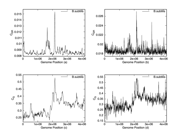
Figure 1: Plot of the iCorr and gCorr values for B. subtilis (NC_000964). (a) $C_{GR}$ vs. genome position with window size = 50,000 and shift size = 10,000. (b) $C_{GR}$ vs. genome position with window size = 10,000 and shift size = 2,000. (c) $C_{G}$ vs. genome position with window size = 50,000 and shift size = 10,000. (d) $C_{G}$ vs. genome position with window size = 10,000 and shift size = 2,000. In (a) and (b), the ORI location is given by the location of peak. In (c) and (d), the ORI location is given by the region where $C_{G}$ undergoes an abrupt change. Clearly, the prediction of iCorr method is much more precise and unambiguous compared to the gCorr method.

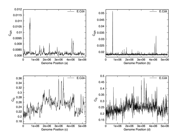
Figure 2: Plot of the gCorr and iCorr values for E. coli (NC_017626) (a) $C_{GR}$ vs. genome position with window size = 50,000 and shift size = 10,000. (b) $C_{GR}$ vs. genome position with window size = 10,000 and shift size = 2,000. (c) $C_{G}$ vs. genome position with window size = 50,000 and shift size = 10,000. (d) $C_{G}$ vs. genome position with window size = 10,000 and shift size = 2,000. In (a) and (b), the ORI location is given by the location of peak. In (c) and (d), the ORI location is given by the region where $C_{G}$ undergoes an abrupt change. It can be clearly seen that the prediction capability of the gCorr method severely deteriorates as the window size decreases, whereas the iCorr method is able to clearly predict the ORI location for window size=10,000.

For ORI prediction in prokaryotic genomes, AGTC combination of $\left\{+i,+1,-i,-1\right\}$ is used. We calculate the auto-correlation of this generated discrete sequence using the same formula given in Eqs. (1) and (2) $\left(\text{using }\mu_{a}=0,\text{ }\sigma=1\right)$, but now $C(k)$ comes out to be a complex number. However, the final auto-correlation value obtained is still a real number since the RHS of Eq. (2) uses the absolute value (or magnitude) of these complex $C\left(k\right)$ values. This is the iCorr value for prokaryotes (denoted by $C_{GR}$) and plotted against the window number (or genome length). The graph produces a sharp peak as its single global property. We propose that the genome position corresponding to this global maximum contains the solitary origin of replication in prokaryotes.

For ORI prediction in eukaryotic bacteria, AGTC combination of $\left\{-1,+1,-i,+i\right\}$ is used. We again calculate the auto-correlation function, $C\left(k\right)$, of this discrete sequence using Eq. (1). However, for calculating the final correlation value (denoted by $C_{GC}$) of each segment/window, we do a sum of only the real part of $C(k)$ values,

$$C_{GC}=\frac{1}{N-1}\sum_{k=1}^{N-1}\Re\left\{C(k)\right\}$$ (3)

where $\Re\left(\cdot\right)$ stands for real part of the complex quantity within brackets. The genome positions corresponding to the zero-crossings of the values of $C_{GC}$ are proposed to be the ORI locations. In this way, it has some similarity to the GC-skew method (MRAzek and Karlin,, 1998).

It is important to note here that unlike the case of prokaryotes, we do not expect a single computational method to be able to correctly predict ORI locations of all eukaryotic genomes due to a large amount of variation in their statistical properties. We have tested our method for S. cerevisiae for which experimental results are known and hope that this $C_{GC}$ defined above or its modifications will be very useful in predicting the ORI locations of a wide variety of genomes.

III Results

We have applied the method described in the previous section to 38 bacterial genomes obtained from NCBI (NCBI,, 2016) and 16 chromosomes of one eukaryote (S. cerevisiae) obtained from OriDB (Siow et al.,, 2012). In this section, we describe the results obtained.

III.1 ORI prediction for prokaryotes

CHR No.	Experimentally Confirmed ORIs	Window/ Shift size	Accuracy(%)	Seq. Removed(%)	Precision(%)	Undetected Confirmed ORIs	Undetected Close Confirmed ORIs
1	14	5000/1000	11/14=78.57	35.65	20/47=42.55	3	0
2	37	10000/2000	27/37=72.97	32.22	43/90=47.77	10	3
3	21	4000/800	13/21=76.19	33.92	24/95=25.26	8	0
4	51	15000/300	37/51=72.55	31.13	63/123=51.21	14	5
5	22	5000/1000	14/22=63.63	40.52	19/111=17.11	8	3
6	17	3000/500	14/17=82.35	35.18	22/109=20.18	3	1
7	30	10000/2000	20/30=66.67	35.59	30/112=26.78	10	1
8	21	5000/1000	15/21=71.42	36.48	19/121=15.70	6	3
9	15	10000/2000	10/15=66.67	27.39	17/48=35.42	5	3
10	29	10000/2000	20/29=68.96	29.56	31/96=32.29	9	3
11	21	10000/2000	15/21=71.42	39.78	31/69=44.93	6	2
12	32	10000/2000	23/32=71.87	40.74	38/101=37.62	9	2
13	27	10000/2000	22/27=81.48	34.84	37/103=35.92	5	0
14	21	10000/2000	16/21=76.19	35.16	25/75=33.33	5	1
15	27	10000/2000	16/27=59.26	33.21	25/127=19.68	11	2
16	25	10000/2000	17/25=68	36.07	32/97=32.99	8	1

Table 1: Analysis of 16 chromosomes in S. cerevisiae.

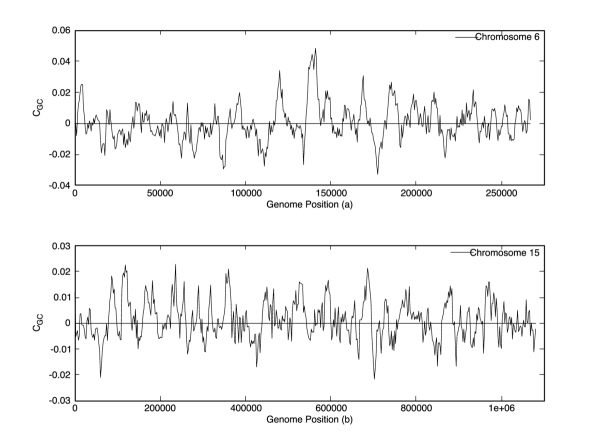
Figure 3: Plot of iCorr vs. genome position for (a) chromosome 6 and (b) chromosome 15 in S. cerevisiae. The points where the graph crosses the zero-line represent possible locations of ORI.

In Figs.1 and 2, (a) and (c) show graphs for iCorr and gCorr method respectively for window size of 50,000 with shift size of 10,000 while (b) and (d) show graphs for window size of 10,000 with shift size of 2,000.

Figure1 (a) and (b) predict ORI location for B. subtilis using iCorr at genome positions 21,70,000 [=217 (window number) × 10,000 (shift size)] and 21,68,000 [=1,084 (window number) × 2,000 (shift size)] respectively, which are very close other. Figure 1 (c) and (d) predict ORI location using gCorr at locations of abrupt change in the genome position ranges of 20,80,000 to 21,60,000 [window number = 208-216] and 21,04,000 to 21,94,000 [window number = 1,057-1,097]. Clearly, both the methods predict common genome locations but iCorr is able to give a more precise result and reduces the genome to be analysed for finding ORI, thereby considerably increasing the resolution.

Figure 2 (a) and (b) predict ORI using iCorr for E. coli at genome positions 5,90,000 [=59 (window number) × 10,000 (shift size)] and 5,88,000 [=294 (window number) × 2,000 (shift size)] respectively, which are very close to each other. Figure 2 (c) predicts ORI using gCorr at locations near 15,00,000-18,00,000 genome position. There is another abrupt change around 42,00,000-43,00,000 genome positions which makes it very difficult to predict one ORI location using auto correlation methods. Figure 2 (d) uses a window size of 10,000 and is extremely noisy and performs very poorly compared to Fig. 2 (c) which uses a window size of 50,000. Therefore, the iCorr method makes a single prediction for ORI location using both window sizes whereas gCorr fails when the window size is small.

gCorr method predicts the presence of ORI in a genome where a sudden transition is observed. The transition spans several windows and its detection depends on human judgement which reduces the accuracy in ORI prediction. In contrast, the iCorr method for prokaryotes predicts the location by finding peak in the graph. Peak is obtained at a single point which helps to narrow down our area of interest to a single window. In the case of B. subtilis, the gCorr predicts the ORI to be present in a genome segment whose length is around 0.1 million (see Fig.1). In contrast, the iCorr method can bring down the range to as low as 0.01 million genome length (20 times higher resolution). This point is strengthened by the fact that the obtained graph deteriorates for gCorr method as the window size is decreased from 50,000 to 10,000 (see Fig. 1 (c), (d) and Fig. 2 (c), (d)). The iCorr is more or less stable and gives a fairly stable peak in the same neighbourhood even when the window size is decreased (see Fig. 1 (a), (b) and Fig. 2 (a), (b)). With the advantages of peak detection and stability with window size, iCorr method is able to predict ORI location with several times more precision than gCorr method.

The peak by average ratio in the iCorr method was found to be in the range $\left(1.2,\text{ }5.4\right)$ with an average of around $1.9$ in the 38 prokaryotic genomes analysed. Out of these 38 genomes, gCorr method failed to make a clear prediction in 10 cases while iCorr faltered in only 4 cases. However, the gCorr and iCorr method predict different ORI locations for the same genome in many cases. In fact, only 4 instances were found to have common prediction location out of the 38 genomes covered. Due to lack of experimental results, we could not verify our predictions to check which of these two methods is correct. It is also possible that many of these genomes have multiple ORI with different statistical properties and hence are captured by different methods.

III.2 ORI prediction for S. cerevisiae

Compared to prokaryotic genomes, the computational prediction of ORI in eukaryotic genomes has been considerably much more challenging due to the rich and complex structure of DNA with multiple ORI being present in a single chromosome. And an added disadvantage is that experimentally verified ORI locations are available for only a few eukaryotes like S. cerevisiae and S. pombe. The predictions made by using gCorr and the peak detection iCorr method described in Sec. II do not match well with the experimental data of these two organisms. So, we have proposed a slightly modified version of peak detection method for this purpose and call it the zero crossing iCorr method. The predictions of this zero crossing method match reasonably well with the known ORI locations of S. cerevisiae. As described in Sec. II, the zero crossing iCorr method uses genome locations of occurrence of zeros instead of the peak locations to predict multiple ORIs. Figure 3 shows the graph of $C_{GC}$ vs. genome location for chromosome 6 and 15 of S. cerevisiae.

We have used different window and sub-window sizes for analysing chromosomes to obtain optimum results (see Table 1). The combination of AGTC used in ORI prediction for S. cerevisiae is $\left\{-1,+1,-i,+i\right\}$ which is different from the combination used in ORI prediction of bacteria. While using sliding window technique, ratio of 5:1 is maintained between window and shift size (only chromosome 6 has a ratio of 6:1). Table 1 summarises the data for the 16 chromosomes analysed. The yeast chromosome sequences and data for their ORI locations was obtained from OriDB (Siow et al.,, 2012).

Below is the explanation to various terms used in Table 1:

• Total Confirmed ORI : Total number of experimentally confirmed ORI found in a chromosome as per the OriDB database.

• Window/ Shift Size : In the sliding window technique, window size is the total size of each window/segment into which the genome is divided (prediction region) and shift size is the step size, i.e., the amount of shift to obtain next window.

• Accuracy : Percentage of experimentally confirmed ORIs (as per OriDB) which are detected by zero-crossing iCorr method. This parameter is basically the hit rate (ratio of computationally detected and experimentally confirmed ORI).

• Sequence Removed : Percentage of sequence which should not contain ORI as per zero-crossing iCorr method. The sum of total length of all such genomic sequence involved in the calculation of window number where the real part of correlation measure changes sign divided by total length of the sequence determines the parameter, “sequence removed”.

• Precision : The method predicts ORI whenever real part of ORI changes sign. This sometimes leads to cases of false prediction, i.e. cases where the method predicts ORI even if no confirmed ORI has been detected. Precision is obtained by dividing the number of zero crossings which actually contain an ORI by the total number of zero crossings. Also, two zero-crossings can sometimes correspond to the same ORI location since our windows/segments have been chosen to be overlapping or sometimes an ORI location can have an overlap with two non-overlapping windows. For the purpose of calculating precision, we count each of these zero-crossings separately even if they point to the same ORI location.

• Undetected Confirmed ORI : The number of confirmed ORIs at which there was no zero crossing of $C_{GC}$.

• Undetected Close Confirmed ORI : Out of the undetected confirmed ORIs, there are some ORIs which are very close to the genome position where real part of correlation measure changes sign. The number of such ORIs lying in the closest forward sub-window from the current window (prediction region) are marked in this column.

As shown in Table 1, the accuracy for all the 16 chromosomes were in the range from 59% to 83% with an average of 71.76%. The method removed 27% to 41% sequence in various chromosomes with an average of 35%. The precision of our prediction lies in the range from 15% to 51% with an average of 32.42%. We believe this to be a good beginning in this relatively challenging area of eukaryotic ORI analysis, specially considering the statistical inference due to the multiple ORI locations.

IV Discussion

In the past, several methods have been developed to predict ORI location for prokaryotes but most of them utilised only a limited amount of information present in the DNA sequence. The GC skew method (MRAzek and Karlin,, 1998) considered frequency counts of G and C nucleotides as the sole means to predict ORI location and neglected the importance of positioning of each base in a DNA sequence. The auto-correlation based gCorr method was developed to remove this inherent flaw of GC skew method by considering relative base positions of the G nucleotide. However, this method was unable to differentiate between A, C and T nucleotides. In an attempt to fully discover the rich variety of bases present in a sequence, we have extended the basic gCorr method to complex states. The iCorr method presented in this paper takes into consideration the relative base positioning of all the four nucleotides. This method has been found to significantly improve the resolution of ORI prediction of prokaryotes and has also been able to predict the ORI locations of S. cerevisiae to a good extent. We also tried to examine the predictions of the iCorr method for another yeast species, S. pombe, but the number of dubious and likely ORI positions covered more than 90% of the total detected ORIs. We hope that we will be able to significantly validate and refine our methods as more experimental data becomes available in the future.

Similar to all the previously existing computational methods, iCorr only suggests the ORI location and does not guarantee existence of ORI. With the advantages of pin-point peak detection and utilisation of rich structure present in DNA, the iCorr method is a significant progress in ORI prediction for prokaryotes. Here it is important to note that the predictions made by these computational methods are significantly dependent on the choice of window/segment size into which the genome is divided for statistical analysis. If the window size is taken to be too large, then the meaningfulness of the predictions obviously goes down. And if the window size is taken to be too small, the graphs can be very noise and lead to decrease in accuracy and precision. For example, in case of chromosomes 8, 9 and 11 of S. cerevisiae, we applied zero-crossing method with window/shift size of 3000/600, 2000/400 and 3000/600 respectively (here, 2000/400 means that the window size is 2000 and shift size is 400) and precision values dropped to 11%, 7% and 13% respectively as compared to the values reported in Table 1.

In the iCorr method for S. cerevisiae, only the zero-crossings of the real part of the correlation measure given by Eq. (3) have been used to predict the ORI locations. It has been observed that the imaginary part of correlation measure remains positive for $>99\%$ of the windows/segments and changes sign at only few isolated contiguous points. This implies that, in some sense, we are observing phase change of the complex correlation values to predict the location of ORI. One interesting observation that we found was the prediction of ORI by gCorr method always yields ORI location around the half-way mark of the genome length. On the other hand, the predictions of ORI by iCorr method doesn’t follow any such pattern. This could be an interesting problem to study in the future and might shed light on the underlying statistical properties of genome sequences.

Author contributions

SK and RL have contributed equally to this work and have carried out the computational work and analysis. KS has designed the research problem and analysed the results. All authors have participated in the article preparation and approved the final article.

References

- McFadden and Roos, (1999) G. I. McFadden and D. S. Roos. "Apicomplexan plastids as drug targets", Trends in Microbiology 7:8, 328-333 (1999). doi: 10.1016/S0966-842X(99)01547-4
- Ram et al., (2007) E. V. S. Raghu Ram et al. "Nuclear gyrB encodes a functional subunit of the Plasmodium falciparum gyrase that is involved in apicoplast DNA replication", Molecular and Biochemical Parasitology 154:1, 30-39 (2007). doi: 10.1016/j.molbiopara.2007.04.001
- Soldati, (1999) D. Soldati. "The apicoplast as a potential therapeutic target in Toxoplasma and other apicomplexan parasites", Parasitology Today 15:1, 5-7 (1999). doi: 10.1016/S0169-4758(98)01363-5
- Marians, (1992) K. J. Marians. "Prokaryotic DNA replication", Annual Review of Biochemistry 61, 673-715 (1992). doi: 10.1146/annurev.bi.61.070192.003325
- Mott and Berger, (2007) M. L. Mott and J. M. Berger. "DNA replication initiation: mechanisms and regulation in bacteria", Nature Reviews Microbiology 5, 343-354 (2007). doi:10.1038/nrmicro1640
- Rocha et al., (1999) E. P. Rocha, A. Danchin and A. Viari. "Universal replication biases in bacteria", Molecular Microbiology 32:1, 11-16 (1999). doi: 10.1046/j.1365-2958.1999.01334.x
- Kelman and Kelman, (2004) L. M. Kelman and Z. Kelman. "Multiple origins of replication in archaea", Trends in microbiology 12:9, 399-401 (2004). doi: 10.1016/j.tim.2004.07.001
- Nasheuer et al., (2002) H. P. Nasheuer et al. "Initiation of eukaryotic DNA replication: regulation and mechanisms", Prog. Nucleic Acid Res. Mol. Biol. 72, 41-94 (2002).
- Sernova and Gelfand, (2008) N. V. Sernova and M. S. Gelfand. "Identification of replication origins in prokaryotic genomes", Briefings in Bioinformatics 9:5, 376-391 (2008). doi: 10.1093/bib/bbn031
- (10) J. R. Lobry. "Asymmetric substitution patterns in the two DNA strands of bacteria", Molecular Biology and Evolution 13:5, 660-665 (1996).
- (11) J. R. Lobry. "Origin of replication of Mycoplasma genitalium", Science 272:5262, 745-746 (1996). doi: 10.1126/science.272.5262.745
- MRAzek and Karlin, (1998) J. Mrazek and S. Karlin. "Strand compositional asymmetry in bacterial and large viral genomes", Proc. Natl. Acad. Sci. USA 95:7, 3720-3725 (1998).
- Touchon et al., (2005) M. Touchon et al. "Replication-associated strand asymmetries in mammalian genomes: toward detection of replication origins", Proc. Natl. Acad. Sci. USA 102:28, 9836-9841 (2005). doi: 10.1073/pnas.0500577102
- Zhang and Zhang, (2005) R. Zhang and C. T. Zhang. "Identification of replication origins in archaeal genomes based on the Z-curve method", Archaea 1:5, 335-346 (2005).
- Grigoriev, (1998) A. Grigoriev. "Analyzing genomes with cumulative skew diagrams", Nucleic Acids Research 26.10, 2286-2290 (1998). doi: 10.1093/nar/26.10.2286
- Chew et al., (2007) D. S. H. Chew, M. Y. Leung and K. P. Choi. "AT excursion: a new approach to predict replication origins in viral genomes by locating AT-rich regions", BMC Bioinformatics 8:163 (2007). doi: 10.1186/1471-2105-8-163
- Schneider, (1997) T. D. Schneider. "Information content of individual genetic sequences", Journal of Theoretical Biology 189:4, 427-441 (1997). doi: 10.1006/jtbi.1997.0540
- Schneider, (2010) T. D. Schneider. "A brief review of molecular information theory", Nano Communication Networks 1:3, 173-180 (2010). doi: 10.1016/j.nancom.2010.09.002
- Shannon, (1948) C. E. Shannon. "A mathematical theory of communication”, Bell Syst. Tech. J. 27:3, 379-423 (1948). doi: 10.1002/j.1538-7305.1948.tb01338.x
- Song et al., (2003) J. Song, A. Ware and S. L. Liu. "Wavelet to predict bacterial ori and ter: a tendency towards a physical balance", BMC genomics 4, 17 (2003). doi: 10.1186/1471-2164-4-17
- Shah and Krishnamachari, (2012) K. Shah and A. Krishnamachari. "Nucleotide correlation based measure for identifying origin of replication in genomic sequences", Biosystems 107, 52-55 (2012). doi: 10.1016/j.biosystems.2011.09.003
- Parikh et al., (2015) H. Parikh et al. "Computational prediction of origin of replication in bacterial genomes using correlated entropy measure (CEM)", Biosystems 128, 19-25 (2015). doi: 10.1016/j.biosystems.2015.01.001
- Li et al., (2014) W. C. Li et al. "Sequence analysis of origins of replication in the Saccharomyces cerevisiae genomes", Frontiers in Microbiology 5, 574 (2014). doi: 10.3389/fmicb.2014.00574
- Lobry and Sueoka, (2002) J. R. Lobry and N. Sueoka. "Asymmetric directional mutation pressures in bacteria", Genome Biology 3:10, research0058.1-14 (2002).
- Mackiewicz et al., (2004) P. Mackiewicz et al. "Where does bacterial replication start? Rules for predicting the oriC region", Nucleic Acids Research 32.13, 3781-3791 (2004). doi: 10.1093/nar/gkh699
- Beauchamp and Yuen, (1979) K. G. Beauchamp and C. K. Yuen. Digital methods for signal analysis (George Allen and Unwin, London, 1979).
- Cavicchi, (2000) T. J. Cavicchi. Digital Signal Processing (John Wiley & Sons, New York, 2000).
- NCBI, (2016) NCBI, Resource Coordinators. "Database resources of the National Center for Biotechnology Information", Nucleic Acids Research 44(D1): D7-19 (2016). doi: 10.1093/nar/gkv1290
- Siow et al., (2012) C. C. Siow et al. "OriDB, the DNA replication origin database updated and extended", Nucleic Acids Research 40 (Database issue): D682-D686 (2012). doi: 10.1093/nar/gkr1091