A Model for Dissipation of Solar Wind Magnetic Turbulence by Kinetic Alfvén Waves at Electron Scales: Comparison with Observations

Abstract

In hydrodynamic turbulence, it is well established that the length of the dissipation scale depends on the energy cascade rate, i.e., the larger the energy input rate per unit mass, the more the turbulent fluctuations need to be driven to increasingly smaller scales to dissipate the larger energy flux. Observations of magnetic spectral energy densities indicate that this intuitive picture is not valid in solar wind turbulence. Dissipation seems to set in at the same length scale for different solar wind conditions independently of the energy flux. To investigate this difference in more detail, we present an analytic dissipation model for solar wind turbulence at electron scales, which we compare with observed spectral densities. Our model combines the energy transport from large to small scales and collisionless damping, which removes energy from the magnetic fluctuations in the kinetic regime. We assume wave-particle interactions of kinetic Alfvén waves (KAW) to be the main damping process. Wave frequencies and damping rates of KAW are obtained from the hot plasma dispersion relation. Our model assumes a critically balanced turbulence, where larger energy cascade rates excite larger parallel wavenumbers for a certain perpendicular wavenumber. If the dissipation is additionally wave driven such that the dissipation rate is proportional to the parallel wavenumber - as with KAW - then an increase of the energy cascade rate is counter-balanced by an increased dissipation rate for the same perpendicular wavenumber leading to a dissipation length independent of the energy cascade rate.

1 Introduction

Turbulence is a common feature in astrophysical and space plasmas, such as the interstellar medium, the solar wind or planetary magnetospheres. Turbulent processes are thought to play an important role in cosmic ray propagation and energetic particle acceleration (e.g., Jokipii, 1966; Bieber et al., 1993, 1996; Farmer & Goldreich, 2004). Furthermore turbulence and the associated dissipative processes could supply energy that is required to explain the non-adiabatic temperature profiles for the plasma species with increasing distance to the sun in the solar wind (Richardson et al., 1995) and increasing distance to the central planet in the respective planetary magnetosphere (Saur, 2004; Bagenal & Delamere, 2011; von Papen et al., 2014). The solar wind serves as a unique laboratory for in-situ measurements of space plasma turbulence thanks to numerous space missions (Bruno & Carbone, 2013). In the past decade, high time resolution magnetic field measurements taken by spacecrafts such as ACE, Cluster, or ARTEMIS led to a flurry of research activity to determine the characteristics of kinetic scale processes. But despite the growing number of observed data sets, there is still insufficient information to fully establish the properties of electron scale processes. Additionally, due to the requirement for a kinetic description at these scales, the interpretation of observations with the help of simulations and theoretical considerations remains particularly difficult. Therefore a number of fundamental physical aspects of small scale solar wind turbulence are still poorly understood.
It is well established that power spectra of magnetic fluctuations at magnetohydrodynamic (MHD) scales follow approximately the Kolmogorov scaling $k^{-5/3}$ (e.g., Matthaeus et al., 1982; Denskat et al., 1983; Horbury et al., 1996; Leamon et al., 1998; Bale et al., 2005). This spectral range is usually called the inertial range of solar wind turbulence. The first clear spectral break appears at ion scales, such as the ion Larmor radius or the ion inertial length (e.g., Leamon et al., 1999; Alexandrova et al., 2008; Chen et al., 2014). At these scales the physical mechanisms change leading to a modification of the cascading process possibly including dissipation, which results in a modified spectral shape. At scales smaller than ion scales, a second cascade range up to electron scales with a steeper slope of about -2.9 to -2.3 is observed (Alexandrova et al., 2009; Kiyani et al., 2009; Chen et al., 2010; Sahraoui et al., 2010), which is called the sub-ion range. Between the inertial range and the sub-ion range a transition region is observed, where the spectra exhibit a power law with a variable spectral index of -4 to -2 (Leamon et al., 1998; Smith et al., 2006; Roberts et al., 2013) or a smooth non power law behavior (Bruno & Trenchi, 2014). The steepening in the transition region has been associated with ion dissipation (Smith et al., 2012) or with the presence of coherent structures (Lion et al., 2016). Even though Helios observations reached into the electron range (Denskat et al., 1983), it was only with the Cluster spacecraft that the electron dissipation range was reached. So far there are only a few observations reported for such small scales with different interpretations (Alexandrova et al., 2009; Sahraoui et al., 2009, 2010; Alexandrova et al., 2012; Sahraoui et al., 2013). A statistical study of magnetic power spectra by Alexandrova et al. (2012) indicate an exponential spectral structure in the dissipation range and a universal behavior for all measured plasma parameters. On the contrary, Cluster observations analyzed by Sahraoui et al. (2013) indicate a third power law at the electron scales with a broad distribution of spectral indices varying from -5.5 to -3.5. This result rather suggests a lack of universality of turbulent fluctuations in the dissipation range, however, the nature of the electron scale spectra and the associated universality remain an open issue.
All these observations appear to be consistent with an important role of kinetic Alfvén waves (KAW). The following picture of a KAW generated turbulent cascade is presented in the literature: In the inertial range nonlinear interactions between Alfvén waves are responsible for the generation of the turbulent cascade. At scales comparable to the ion Larmor radius, the Alfvén wave is possibly slightly damped, which would explain the transition range (Denskat et al., 1983). However, the process that leads to a steepening of the spectrum in the sub-ion range, i.e., between ion and electron scales is the transformation from the non-dispersive Alfvén wave to the dispersive KAW (Howes et al., 2006). The energy in Alfvénic fluctuations generates a dispersive KAW cascade down to the electron scales, which again can be described in fluid-like terms (Schekochihin et al., 2009). In the vicinity of the electron Larmor radius or the electron inertial length, the KAW is subject to strong Landau damping via wave-particle interactions (Gary & Nishimura, 2004; Sahraoui et al., 2009). Since properties of the whistler wave are similar to those of the KAW (e.g., Boldyrev et al., 2013), it is difficult to distinguish these waves in observations. Hence, there is still an ongoing debate whether the small scale fluctuations consist of whistler waves or KAW (Gary & Smith, 2009; Salem et al., 2012; Chen et al., 2013).
Observations with different angles between the mean magnetic field and the solar wind flow direction lead to the understanding that magnetic fluctuations are anisotropic with respect to the mean magnetic field in both the MHD regime (e.g., Barnes, 1979; Matthaeus et al., 1990; Bieber et al., 1996; Horbury et al., 2008) and the kinetic regime (e.g., Chen et al., 2010; Sahraoui et al., 2010; Narita et al., 2011). Goldreich & Sridhar (1995) proposed a particular model for the anisotropy, called critical balance, which leads to observed $P(k_{\perp})\propto k_{\perp}^{-5/3}$ and $P(k_{\parallel})\propto k_{\parallel}^{-2}$ spectra in the inertial range (Horbury et al., 2008; Podesta, 2009). By equating the nonlinear timescale at which the energy is transferred to smaller scales with the linear Alfvén timescale, one finds $k_{\parallel}\propto k_{\perp}^{2/3}$ in the inertial range and $k_{\parallel}\propto k_{\perp}^{1/3}$ in the kinetic range (Cho & Lazarian, 2004; Schekochihin et al., 2009). Hence, the turbulence becomes more anisotropic for high wavenumbers and the energy is cascaded mainly in the perpendicular direction $k_{\perp}\gg k_{\parallel}$. Although recent observations and simulations are consistent with the critical balance assumption (TenBarge & Howes, 2012; He et al., 2013; von Papen & Saur, 2015), its applicability to solar wind turbulence is still subject of debate and other models are proposed to explain the anisotropy (Narita et al., 2010; Li et al., 2011; Horbury et al., 2012; Wang et al., 2014; Narita, 2015).
A surprising result in the observation by Alexandrova et al. (2012) is the independence of the dissipation length from the amplitude of the turbulent spectra $P_{0}$ at a fixed wavenumber $k_{0}$. This independence is a remarkable difference compared to hydrodynamic turbulence, where the dissipation length $l_{d,\mathrm{Kolm}}=(\nu^{3}/\varepsilon_{0})^{1/4}$ is given by the energy cascade rate $\varepsilon_{0}$ and the kinematic viscosity $\nu$ (e.g., Frisch, 1995). Accordingly, in hydrodynamic turbulence, the more energy is injected per unit mass, the more the turbulence is driven to smaller scales to dissipate the larger energy flux. Following Kolmogorov (1941), the amplitude of the turbulent spectra and the energy cascade rate are related by $\varepsilon_{0}\propto P_{0}^{3/2}k_{0}^{5/2}$. The solar wind observations by Alexandrova et al. (2012) show approximately no dependence of the dissipation length on the energy cascade rate. This is indeed surprising under the assumption that the energy is not fully dissipated at a resonance, but that the dissipation rate $\gamma$ is a smooth function of wavenumber $k$ such as, e.g., for Landau damping of KAW (Lysak & Lotko, 1996; Howes et al., 2006; Sahraoui et al., 2012; Narita & Marsch, 2015). In this case, one would still expect that a larger energy flux drives the turbulence to smaller scales before the energy is dissipated. This effect is neither noted nor discussed in earlier dissipation models by Howes et al. (2008); Podesta et al. (2010); Howes et al. (2011), although the independence of the dissipation length scale from the energy cascade rate is implicitly included in these models. To discuss this issue in detail, we present a ’quasi’ analytical dissipation model to describe magnetic power spectra at sub-ion scales. The model is tailored to be applied for data comparison with variable spectral slope and associated critical balance. For the description of the turbulent energy transport, we introduce in Section 2 a cascade model, which is in several aspects similar to earlier turbulence models (e.g., Pao, 1965; Howes et al., 2008; Podesta et al., 2010; Zhao et al., 2013). Still, we give a short derivation of our model equation in order to establish a basis for theoretical predictions of solar wind dissipation processes and to discuss the independence of the dissipation length from the energy cascade rate. As a damping rate, we include the imaginary part of the KAW wave frequency obtained from linear Vlasov theory. In Section 2.3, we investigate the dissipation length scale and the spectral shape of the dissipation range under the assumption of linear KAW damping and critically balanced turbulence. In Section 3, we present a statistical study, where we fit an exponential function proposed by Alexandrova et al. (2012) to 300 model spectra for varying solar wind conditions. In Section 4, we discuss the limitations of our approach and of the resultant implications for solar wind dissipation.

2 MODEL FOR MAGNETIC ENERGY SPECTRA

In this section, we construct a dissipation model for energy spectra of turbulent fluctuations. The model is a linear combination of the nonlinear transport of energy from the large to the small scales and the dissipation process at small scales. In its general form, the model can in principle describe turbulent spectra in any plasma or fluid. For solar wind turbulence we assume a critically balanced energy cascade of KAWs up to the highest wavenumbers where the energy is dissipated by wave-particle interactions. Turbulent dissipation is quantified by the imaginary part of the wave frequency obtained from a dispersion relation for KAWs. Note that similar to common terminology in previous publications, the term ”dissipation” refers in this paper to the transfer of energy from the magnetic field into perturbations of the particle distribution function via wave-particle interactions. The final transfer of this non-thermal free energy in the distribution function to thermal energy, i.e, the irreversible thermodynamic heating of the plasma, can only be achieved by collisions (Schekochihin et al., 2009; Howes, 2015; Schekochihin et al., 2016).

2.1 Energy Cascade and Dissipation

Based on the idea that the turbulent energy cascades self-similarly to higher wavenumbers (Frisch, 1995), we write the energy cascade rate as

$$\varepsilon(k)=C_{K}^{-3/2}P(k)v_{k}(k),$$ (1)

where $P(k)$ defines the spectral energy density of magnetic fluctuations and $C_{K}$ is the dimensionless Kolmogorov constant. We introduce the ’velocity’ of the energy transport in wavenumber space or ’eddy-decay velocity’ $v_{k}(k)=dk/dt$. In the inertial range, the energy cascade rate $\varepsilon_{0}$ is constant, i.e., the energy is transported loss-free from large to small scales. In this case, (1) can be written as

$$\varepsilon_{0}=C_{K}^{-3/2}P_{0}v_{k0}=\mbox{const.,}$$ (2)

where $P_{0}=P(k_{0})$ and $v_{k0}=v_{k}(k_{0})$ characterize the spectral properties at a wavenumber $k_{0}$ in the inertial range. The fluid velocity $v$ and the eddy-decay velocity of magnetic fluctuations $v_{k}$ are related by

$$v_{k}(k)=\frac{dk}{dt}=k^{2}v(k).$$ (3)

The ratio of velocity to magnetic fluctuations $\alpha$ is assumed to be (Schekochihin et al., 2009)

$$v(k)=\alpha\sqrt{\frac{P(k)k}{\rho}},$$ (4)

with the mass density $\rho$. From (1), (3), and (4), we obtain

$$P(k)=C_{K}\rho^{1/3}\varepsilon(k)^{2/3}\alpha(k)^{-2/3}k^{-5/3}.$$ (5)

Assuming $\alpha$ to follow a power law of the form $\alpha=\alpha_{0}(k/k_{0})^{\beta}$, we can write $P(k)$ as

$$P(k)=P_{0}\left(\frac{\varepsilon(k)}{\varepsilon_{0}}\right)^{2/3}\left(\frac{k}{k_{0}}\right)^{-\kappa},$$ (6)

with $\kappa=2/3\beta+5/3$. With (1), (2), and (6), we write the eddy-decay velocity $v_{k}(k)$ as:

$$v_{k}(k)=v_{k0}\left(\frac{\varepsilon(k)}{\varepsilon_{0}}\right)^{1/3}\left(\frac{k}{k_{0}}\right)^{\kappa}.$$ (7)

Due to dissipation, the energy flux at wavenumber $k^{\prime}=k+dk$ differs from the energy flux at $k$ by the part of energy $D(k)dk$ that is dissipated

$$C_{K}^{-3/2}P(k)v_{k}(k)=C_{K}^{-3/2}P(k^{\prime})v_{k}(k^{\prime})+D(k)dk.$$ (8)

The heating rate $D(k)=2P(k)\gamma(k)$ contains a damping rate $\gamma(k)$. From (6), (7), (8), and a Taylor expansion of $P(k^{\prime})v_{k}(k^{\prime})$ for small $dk$ in equation (8), we obtain a differential equation for the energy spectrum of turbulent fluctuations $P(k)$

$$\frac{dP(k)}{dk}=-P(k)\left(\frac{\kappa}{k}+\frac{4}{3}C_{K}^{3/2}\frac{\gamma(k)}{v_{k}(k)}\right).$$ (9)

The solution of (9) for $P(k)$ yields the one-dimensional energy spectrum

$$P(k)= P_{0}\left(\frac{k}{k_{0}}\right)^{-\kappa}\exp\left(-\frac{4}{3}C_{K}^{3/2}\right.$$

$$\times\left.\int_{k_{0}}^{k}dk^{\prime}\frac{\gamma(k^{\prime})}{v_{k}(k^{\prime})}\right).$$ (10)

Insertion of (1) and (5) in (10) leads to

$$P(k)= P_{0}\left(\frac{k}{k_{0}}\right)^{-\kappa}\exp\left(-\frac{4}{3}C_{K}\int_{k_{0}}^{k}dk^{\prime}\left(\frac{\varepsilon(k^{\prime})}{\rho}\right)^{-1/3}\right.$$

$$\left.\times\,\alpha(k^{\prime})^{-2/3}\gamma(k^{\prime})k^{\prime-5/3}\right).$$ (11)

With (6), equation (11) can be written in terms of the energy flux

$$\varepsilon(k)= \varepsilon_{0}\exp\left(-2C_{K}\int_{k_{0}}^{k}dk^{\prime}\left(\frac{\varepsilon(k^{\prime})}{\rho}\right)^{-1/3}\right.$$

$$\times\,\left.\alpha(k^{\prime})^{-2/3}\gamma(k^{\prime})k^{\prime-5/3}\right).$$ (12)

Under the assumption that the eddy-decay velocity is not affected by the dissipation

$$v_{k}(k)\approx v_{k0}\left(\frac{k}{k_{0}}\right)^{\kappa},$$ (13)

and using (2) and (5), equation (10) simplifies to

$$P(k)= P_{0}\left(\frac{k}{k_{0}}\right)^{-\kappa}\exp\left(-\frac{4}{3}C_{K}\left(\frac{\varepsilon_{0}}{\rho}\right)^{-1/3}\alpha_{0}^{-2/3}\right.$$

$$\times\,\left.k_{0}^{-5/3}\int_{k_{0}}^{k}dk^{\prime}\gamma(k^{\prime})\left(\frac{k^{\prime}}{k_{0}}\right)^{-\kappa}\right).$$ (14)

Turning to hydrodynamic turbulence and insertion of a resistive damping rate $\gamma(k)=\nu k^{2}$ with the kinematic viscosity $\nu$, which is valid in a collisional fluid (e.g., Drake, 2006), we can use our model to calculate the associated energy spectrum. When we assume that the eddy-decay velocity is not affected by the damping as in (13), we find

$$P(k)=P_{0}\left(\frac{k}{k_{0}}\right)^{-5/3}\exp\left(-C_{K}\nu\left(\frac{\varepsilon_{0}}{\rho}\right)^{-1/3}k^{4/3}\right),$$ (15)

where we use $\kappa=5/3$, $k_{0}\ll k$, $\alpha_{0}=1$, and where $P(k)$ denotes the energy density of velocity fluctuations in this case. This spectral form has been found previously by Corrsin (1964) and Pao (1965). Equating the length scale, where the argument of the exponential function in equation (15) assumes -1, we obtain the dissipation scale for hydrodynamic turbulence

$$l_{d,hd}=C_{K}^{3/4}\left(\frac{\nu^{3}\rho}{\varepsilon_{0}}\right)^{1/4},$$ (16)

which is apart from constant factors on the order of unity in agreement with the Kolmogorov dissipation scale $l_{d,\mathrm{Kolm}}\sim(\nu^{3}/\varepsilon_{0}^{*})^{1/4}$ with the cascade rate per unit mass $\varepsilon_{0}^{*}=\varepsilon_{0}/\rho$. Assuming alternatively that the eddy-decay velocity is slowed down by the damping in the dissipation range according to (7), we find an algebraic spectral energy density

$$P(k)=P_{0}\left(\frac{k}{k_{0}}\right)^{-5/3}\left(1-\frac{1}{2}C_{K}\left(l_{d,hd}k\right)^{4/3}\right)^{2},$$ (17)

where we again use $\kappa=5/3$, $k_{0}\ll k$, and $\alpha_{0}=1$. $P(k)$ decreases more rapidly compared to the previous case and vanishes at a maximum wavenumber. A similar spectral form has been found by Kovasznay (1948). Expressions (15) and (17) provide models how the dissipation and the associated dissipation length depend on the energy flux in hydrodynamic turbulence. Consequences resulting from this fact and differences to solar wind turbulence will be discussed in Section 2.3.
For KAWs, we include the normalized damping rate

$$\gamma(k_{\perp},k_{\parallel})=k_{\parallel}v_{A}\overline{\gamma}(k_{\perp},k_{\parallel}),$$ (18)

which is the imaginary part of the complex wave frequency in the dispersion relation for KAWs with $\omega=\omega_{r}+\mathrm{i}\gamma$ and the Alfvén velocity $v_{A}=B_{0}/\sqrt{\mu_{0}\rho}$. We assume that the linear Alfvén time scale and the nonlinear time scale are equal at all scales. This equality is the critical balance assumption of Goldreich & Sridhar (1995), which leads to a relation between $k_{\parallel}$ and $k_{\perp}$

$$v_{\perp}(k_{\perp})k_{\perp}=k_{\parallel}v_{ph,A}=k_{\parallel}v_{A}\overline{\omega}_{r},$$ (19)

where $v_{\perp}$ is the plasma velocity perpendicular to the mean magnetic field, which we take in the remainder as the turbulent velocity fluctuations introduced in (3) and (4), $v_{ph,A}=v_{A}\overline{\omega}_{r}$ is the phase velocity of the wave, and $\overline{\omega}_{r}=\omega_{r}/k_{\parallel}v_{A}$ is the real part of the normalized wave frequency describing the deviations from the MHD shear Alfvén wave. From (1), (3), (5), and (19), we obtain an equation for the parallel wavenumber as a function of the perpendicular wavenumber

$$k_{\parallel}=C_{K}^{1/2}(v_{A}\overline{\omega}_{r})^{-1}\left(\frac{\varepsilon(k_{\perp})}{\rho}\right)^{1/3}\alpha(k_{\perp})^{2/3}k_{\perp}^{2/3}.$$ (20)

For $\alpha(k_{\perp})\approx\overline{\omega}_{r}$ (Howes et al., 2008) and without dissipation ($\varepsilon(k_{\perp})=\varepsilon_{0}$), (20) leads to the typical relations for $k_{\parallel}$ and $k_{\perp}$ as discussed in the introduction in both the MHD regime ($\overline{\omega}_{r}\approx 1$) and the kinetic regime ($\overline{\omega}_{r}\approx k_{\perp}\rho_{i}$). Inclusion of (18) and (20) into (11) yields the perpendicular energy spectrum for magnetic fluctuations

$$P(k_{\perp})= P_{0}\left(\frac{k_{\perp}}{k_{0}}\right)^{-\kappa}\exp\left(-\frac{4}{3}C_{K}^{3/2}\right.$$

$$\times\,\left.\int_{k_{0}}^{k_{\perp}}dk_{\perp}^{\prime}\frac{\overline{\gamma}(k_{\perp}^{\prime},k_{\parallel})}{\overline{\omega}_{r}(k_{\perp}^{\prime},k_{\parallel})}k_{\perp}^{\prime-1}\right).$$ (21)

Again with (6), equation (21) can be expressed in terms of the energy flux

$$\varepsilon(k_{\perp})=\varepsilon_{0}\exp\left(-2C_{K}^{3/2}\int_{k_{0}}^{k_{\perp}}dk_{\perp}^{\prime}\frac{\overline{\gamma}(k_{\perp}^{\prime},k_{\parallel})}{\overline{\omega}_{r}(k_{\perp}^{\prime},k_{\parallel})}k_{\perp}^{\prime-1}\right).$$ (22)

The latter expression is apart from constant factors similar to the dissipation model proposed by Howes et al. (2008). From (3), (10), (18), and (19), we see that the energy spectrum in (21) and the associated energy flux in (22) are independent of the choice of the eddy-decay velocity in the dissipation range, i.e., it leads to the same results for (7) and (13).

2.2 Damping Rates of Kinetic Alfvén Waves

In this section, we present the calculation of damping rates obtained from the hot plasma dispersion relation for a nonrelativistic plasma with Maxwellian distributed electrons and protons with no zero-order drift velocities. The hot plasma dispersion relation refers to the general relationship arising from the set of linearized Vlasov Maxwell equations (e.g., Stix, 1992)

$$\mathrm{det}\left[{\bf k}\otimes{\bf k}-k^{2}\mathbbm{1}+\frac{\omega^{2}}{c^{2}}\underline{\underline{\epsilon}}\right]=0,$$ (23)

where $\mathbbm{1}$ denotes the identity matrix, $c$ the speed of light, and $\epsilon_{ij}$ the elements of the dielectric tensor (see Appendix A.1 for a description of the dielectric tensor elements and definitions of all symbols). Assuming that the wave vector is in the $xz$ plane, the dispersion relation can be written in the form

$$\mathrm{det}\left(\begin{array}[]{ccc}\epsilon_{xx}-n_{\parallel}^{2}&\epsilon_{xy}&\epsilon_{xz}+n_{\parallel}n_{\perp}\\ -\epsilon_{xy}&\epsilon_{yy}-n^{2}&\epsilon_{yz}\\ \epsilon_{xz}+n_{\parallel}n_{\perp}&-\epsilon_{yz}&\epsilon_{zz}-n_{\perp}^{2}\end{array}\right)=0,$$ (27)

with the parallel, perpendicular and total index of refraction $n_{\parallel}=k_{\parallel}c/\omega$, $n_{\perp}=k_{\perp}c/\omega$ and $n=k\omega/c$, respectively. From equation (27), we obtain the wave frequency as a complex number, $\omega=\omega_{r}+\mathrm{i}\gamma$. Details of the numerical evaluation are given in Appendix A.2.
We compare the resultant damping rates with two other damping rates for KAW: Damping rates obtained from the hot dispersion relation with the Padé approximation for the plasma dispersion function $Z(\xi)$, which is used in other dispersion relation solvers (e.g., Rönnmark, 1982; Narita & Marsch, 2015), and damping rates from a simplified algebraic dispersion relation found by Lysak & Lotko (1996), which was derived to describe low-frequency waves in small plasma beta plasmas, e.g., the Earth’s magnetosphere. The advantage of both methods are much faster computation times of the root finding algorithm in comparison to the hot dispersion relation solver. For low-frequency waves ($\omega\ll\Omega_{s}=q_{s}B/m_{s}$, with gyrofrequency $\Omega_{s}$, particle charge $q_{s}$ and particle mass $m_{s}$ for species $s$), large parallel wavelength ($k_{\parallel}v_{s}\ll\Omega_{s}$, with thermal velocity $v_{s}$), and small plasma betas ($\beta_{s}=2k_{B}T_{s}n_{s}\mu_{0}/B^{2}\ll 1$, with temperature $T_{s}$ and number density $n_{s}$) the full system of the hot dispersion relation can be approximated by a $2\times 2$ matrix since the fast mode can be factored out. Then the determinant of the $2\times 2$ matrix yields the dispersion relation (Lysak & Lotko, 1996)

$$\frac{\omega^{2}}{k_{\parallel}^{2}v_{A}^{2}}=\frac{k_{\perp}^{2}\rho_{i}^{2}}{1-\Gamma_{0}(k_{\perp}^{2}\rho_{i}^{2})}+\frac{k_{\perp}^{2}\rho_{a}^{2}}{\Gamma_{0}(k_{\perp}^{2}\rho_{e}^{2})\left[1+\xi Z(\xi)\right]},$$ (28)

with the gyroradius $\rho_{s}=v_{s}/\Omega_{s}$ and the ion acoustic gyroradius $\rho_{a}^{2}=k_{B}T_{e}/m_{i}\Omega_{i}^{2}$ (see Appendix A.1 for definitions of all other symbols). Note that $\xi=\xi(\omega)$; thus, equation (28) is an implicit equation for the normalized wave frequency $\overline{\omega}=\overline{\omega}_{r}+\mbox{i}\overline{\gamma}$, which can be solved numerically. Figure 1 shows normalized damping rates ($\overline{\gamma}/\overline{\omega}_{r}$) calculated from the hot dispersion relation (solid lines), the hot dispersion relation with Padé approximation (dotted lines), and the Lysak & Lotko (1996) approximation (dashed lines) for temperature ratios of $T_{i}/T_{e}=1$ (panel (a)) and $T_{i}/T_{e}=10$ (panel (b)) for ion plasma beta values of 0.01, 0.1, 1, and 10. The ratio of $k_{\parallel}$ to $k_{\perp}$ is given through the critical balance condition in (20). We use typical solar wind values for the magnetic field (10 nT) and the electron number density (10 cm^-3).

Figure 1: $\overline{\gamma}/\overline{\omega}_{r}$ for a temperature ratio of $T_{i}/T_{e}=1$ (a) and of $T_{i}/T_{e}=10$ (b) and ion plasma betas of 0.01, 0.1, 1.0 and 10.0. Damping rates from the simplified dispersion relation are shown in dashed lines, hot damping rates in solid lines and hot damping rates with Padé approximation in dotted lines.

For all values of $\beta_{i}$, hot damping rates with Padé approximation are in agreement with hot damping rates for $k_{\perp}\rho_{i}>1$, but show small errors when the wave frequency is almost real and $\gamma$ is nearly negligibly small. Due to critical balance, the real part of the wave frequency does not reach the ion gyrofrequency where differences of the plasma dispersion function and the Padé approximation would occur. Damping rates calculated with the Lysak & Lotko (1996) approximation show good agreement with hot damping rates for $\beta_{i}=0.01$ and $\beta_{i}=0.1$. Small deviations occur at $k_{\perp}\rho_{i}\approx 10$, where $\omega_{r}$ comes closer to the ion gyrofrequency. For $\beta_{i}\geq 1$, both the amplitude and the general form of the damping rates calculated with the Lysak & Lotko (1996) approximation differ significantly from hot damping rates already for scales $k_{\perp}\rho_{i}<1$. The results confirm that the Lysak & Lotko (1996) dispersion relation can be well applied for $\beta_{i}\ll 1,~{}\beta_{e}\ll 1$ and $\omega_{r}\ll\Omega_{i}$. Although the simplified dispersion relation is valid for a range of solar wind parameters, quantitative conclusions concerning damping at electron scales cannot be drawn. For a complete analysis of dissipation processes under the full parameter space of the solar wind conditions usage of the hot dispersion relation is necessary.

2.3 Implications for the Dissipation Range

With our model for the spectral energy density in equation (21) we can draw conclusions about the dissipation length and the spectral shape of the solar wind dissipation range. Let us first look at the critical balance assumption in (20) again. Equation (20) reveals the dependence of the parallel wavenumber on the energy flux $\varepsilon(k_{\perp})$. Consequently, $\gamma(k_{\perp},k_{\parallel})$ depends on $\varepsilon(k_{\perp})$ as well. Returning to the general spectral form in equation (11), we see that $\varepsilon(k_{\perp})$ cancels under the assumption of critical balance so that the dissipation is not explicitly dependent on $\varepsilon(k_{\perp})$. However, $\overline{\omega}_{r}=\omega_{r}/k_{\parallel}v_{A}$ and $\overline{\gamma}=\gamma/k_{\parallel}v_{A}$ in (21) can be explicit functions of $k_{\parallel}$, if $\gamma(k_{\perp},k_{\parallel})$ and $\omega_{r}(k_{\perp},k_{\parallel})$ are nonlinear functions of $k_{\parallel}$. Damping rates calculated from the Lysak & Lotko (1996) approximation in (28) satisfy the condition $\overline{\gamma}(k_{\perp})=\gamma(k_{\perp},k_{\parallel})/k_{\parallel}v_{A}$ exactly leading to a dissipation which is independent of the energy flux and hence to the same dissipation scale for different values of the energy flux. For normalized damping rates for KAW obtained from the hot plasma dispersion relation, the independence of $\overline{\gamma}$ from the parallel wavenumber cannot be shown analytically but can be estimated numerically. Figure 2 shows the parallel wavenumber as a function of the perpendicular wavenumber as derived in equation (20) and (12) for four different values of $\varepsilon_{0}$. The dotted line denotes the first spectral break at ion scales. The break frequency and the original value of $\varepsilon_{0}=7\times 10^{-16}\ \rm Jm^{-3}s^{-1}$ are taken from observation 5 in Alexandrova et al. (2009).

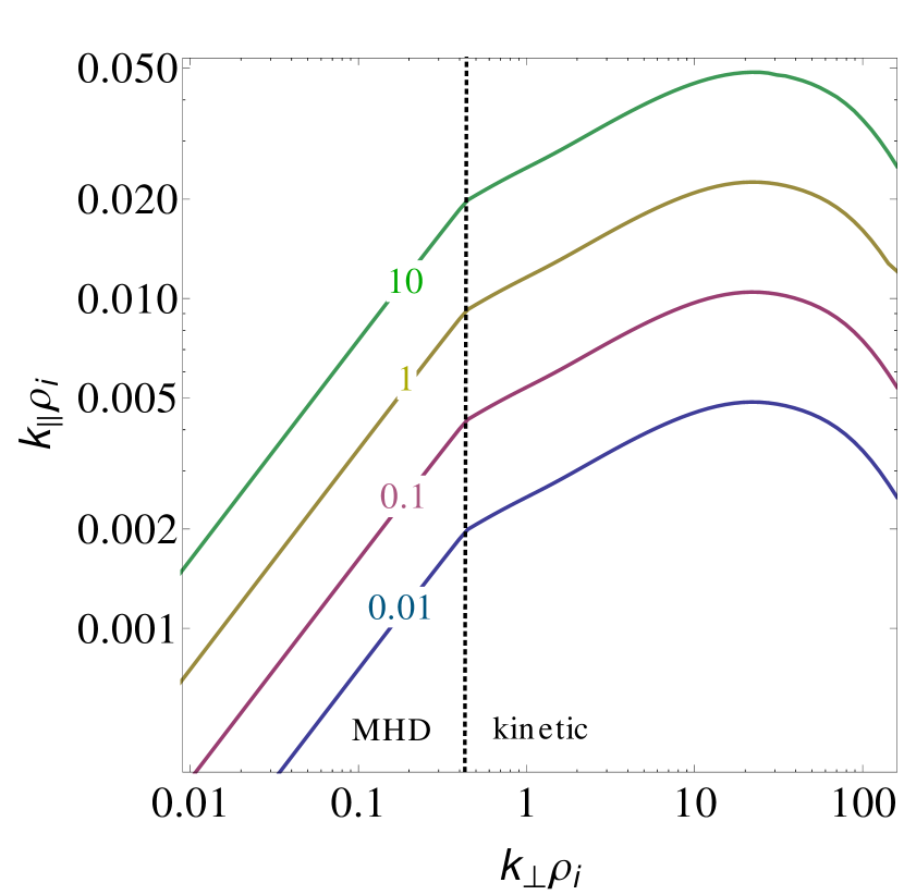
Figure 2: Equation (20) for $\varepsilon_{0}=\{0.01,0.1,1,10\}\times\varepsilon_{0,\mathrm{ref}}$ with $\varepsilon_{0,\mathrm{ref}}=7\times 10^{-16}\ \rm Jm^{-3}s^{-1}$ calculated from Alexandrova et al. (2009). The dotted line shows the transition from MHD to the kinetic regime. Solar wind parameters ($B=15.5$ nT, $n=20$ cm^-3, $T_{i}=61$ eV, $T_{e}=26$ eV, and $v_{S}=630$ km/s), the break frequency, and $\varepsilon_{0,\mathrm{ref}}$ are taken from observation 5 in Alexandrova et al. (2009).

The larger $\varepsilon_{0}$, the more the turbulence generates large parallel wavenumbers for the same perpendicular wavenumber. Figure 3 shows the hot damping rate ($\overline{\gamma}/\overline{\omega}_{r}$) for all ratios of $k_{\parallel}$ to $k_{\perp}$ from Figure 2. All damping rates fall approximately on the same dark blue solid line. $\overline{\gamma}/\overline{\omega}_{r}$ from the Lysak & Lotko (1996) approximation is shown in the dashed line for comparison. At least for typical solar wind parameters, the normalized hot damping rates for KAW are also approximately independent of the parallel wavenumber: $\overline{\gamma}(k_{\perp},k_{\parallel})/\overline{\omega}_{r}(k_{\perp},k_{\parallel})\sim\overline{\gamma}(k_{\perp})/\overline{\omega}_{r}(k_{\perp})$, which leads again to the same dissipation scale for all spectra independently of the injected energy rate.

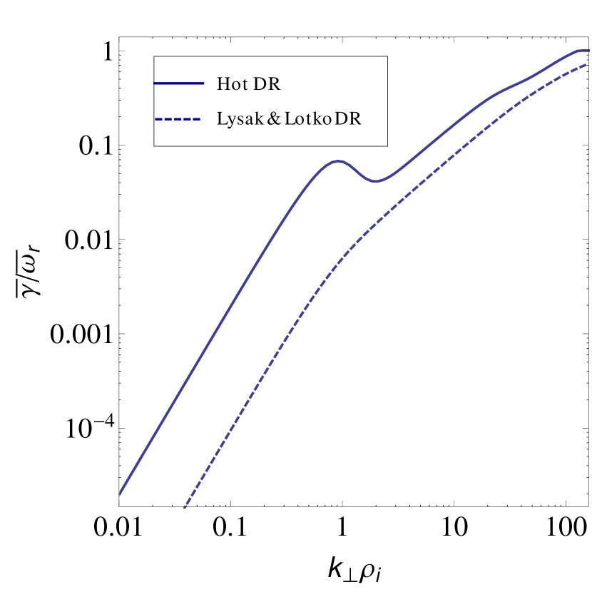
Figure 3: Hot damping rate ($\overline{\gamma}/\overline{\omega}_{r}$) for all ratios of $k_{\parallel}$ to $k_{\perp}$ from Figure 2 and the same parameters as in Figure 2. All damping rates fall approximately on the same dark blue solid line. $\overline{\gamma}/\overline{\omega}_{r}$ from the Lysak & Lotko (1996) approximation is shown in the dashed line for comparison.

We can estimate this dissipation scale for solar wind turbulence similar to the HD Kolmogorov dissipation scale by equating the argument of the exponential term in equation (22) with -1, i.e., where the energy flux is reduced by the factor of $1/e$ and the difference is converted into heat or other forms of particle acceleration

$$1=2C_{K}^{3/2}\int_{k_{0}}^{k_{\perp}}k_{\perp}^{\prime-1}\frac{\overline{\gamma}}{\overline{\omega}_{r}}(k_{\perp}^{\prime})dk_{\perp}^{\prime}.$$ (29)

Up to this scale the dissipation term is negligible or small compared to the spectral energy transport. When we assume for mathematical simplicity the normalized damping rate to be in the form of a power law $\overline{\gamma}/\overline{\omega}_{r}\propto k_{\perp}^{\zeta}$, the integral in equation (29) can be solved analytically:

$$1=2C_{K}^{3/2}\zeta^{-1}\overline{\gamma}/\overline{\omega}_{r}$$ (30)

$$\Rightarrow\overline{\gamma}(k_{d})/\overline{\omega}_{r}(k_{d})\sim 1.$$ (31)

Hence, dissipation sets in at scales $k_{d}=1/l_{d}$ where the damping rate equals the real frequency independently of the energy cascade rate.
The differences of the solar wind dissipation length in comparison to the hydrodynamic dissipation length

     Hydrodynamic Turbulence      

     Solar Wind Turbulence g    

Figure 4: Sketch of the role of different energy cascade rates on the energy distribution in k-space (left panels) and on the energy flux $\varepsilon(k)$ (right panel) for hydrodynamic turbulence (top panels) and solar wind turbulence (bottom panels). The different values for the energy cascade rate $\varepsilon_{0}$ are referred to as $\varepsilon_{1}$, $\varepsilon_{2}$, $\varepsilon_{3}$ with $\varepsilon_{1}<\varepsilon_{2}<\varepsilon_{3}$. In panel (c), the energy distribution for solar wind turbulence is assumed to follow critical balance, which implies that larger $\varepsilon_{0}$ result in larger parallel wavenumbers $k_{\parallel}$. For KAW larger parallel wavenumbers additionally result in larger damping rates $\gamma$ for the same $k_{\perp}$. The larger damping rates $\gamma$ are indicated by the intensity of the red color in panel (c). The dissipation scales $k_{d}$ shown in orange in panel (b) and (d) are defined as the scales where the energy is reduced by a factor of $1/e$.

are sketched in Figure 4. Top panels show the hydrodynamic case, bottom panels show the solar wind case. Panel (a) displays the isotropic energy distribution in HD turbulence and panel (c) shows the anisotropic energy distribution in a magnetized plasma under the assumption of critical balance for different values of $\varepsilon_{0}$ labeled $\varepsilon_{3}>\varepsilon_{2}>\varepsilon_{1}$.Panel (c) shows additionally in red the general intensity of damping for different $\varepsilon_{0}$ for linear wave mode damping such as in our KAW model.In a critically balanced turbulence, larger values of $\varepsilon_{0}$ lead to larger parallel wavenumbers (see equations (18) and (20)). The larger parallel wavenumbers at a given perpendicular wavenumber lead to larger damping rates. In contrast in HD turbulence, $\varepsilon_{0}$ has no influence on the damping rate $\gamma(k)=\nu k^{2}$. Following equation (12), panels (b) and (d) illustrate schematically the influence of different values of $\varepsilon_{0}$ ($\varepsilon_{2}>\varepsilon_{1}$) on the energy cascade rate $\varepsilon(k)$ and $\varepsilon(k_{\perp})$ for hydrodynamic turbulence and solar wind turbulence, respectively. The dissipation length, marked by the orange dashed lines, is defined as the scale where the energy flux is reduced by a factor of $1/e$. For HD turbulence, larger $\varepsilon_{0}$ leads to a smaller dissipation scale, whereas the dissipation length in the solar wind plasma is independent of the energy flux. To explain this difference in detail, we look at the equation that describes the relative change of the energy flux (derived from (12)

$$\frac{1}{\varepsilon(k)}\frac{d\varepsilon(k)}{dk}\propto-\left(\frac{\varepsilon(k)}{\rho}\right)^{-1/3}\gamma(k)k^{-\kappa}.$$ (32)

For resistive HD damping the relative change of energy flux , i.e., $1/\varepsilon(k)\ d\varepsilon/dk=d/dk\ \ln\varepsilon(k)$ on the left hand side of (32) depends on $\varepsilon(k)^{-1/3}$ and therefore on the energy injection rate $\varepsilon_{0}$. The relative change of the energy flux therefore changes depending on how strongly the turbulence is driven. Different $\varepsilon_{0}$ result in different amplitudes of the energy spectrum as well as in different exponential curves in HD turbulence. In the case of solar wind turbulence under the assumption of a critically balanced energy distribution the situation is different. A larger energy flux leads to a modified anisotropic distribution of energy in k-space, i.e., larger $k_{\parallel}$ for the same $k_{\perp}$ (see Figure 4(c)). These larger parallel wavenumbers result in larger damping rates $\gamma\sim k_{\parallel}v_{A}\overline{\gamma}(k_{\perp})\sim\varepsilon(k_{\perp})^{1/3}\overline{\gamma}(k_{\perp})$ (see colored lines and related color bar in Figure 4 (c)). By insertion of $\gamma(k)$ into (32), we see that the right hand side of (32) is independent of the energy flux $\varepsilon(k_{\perp})$. Therefore the relative change of the energy density and the spectral form of the energy density is independent of $\varepsilon_{0}$. The larger energy flux, which drives the turbulent energy to smaller scales, is compensated by the larger damping rates. This compensation of a larger energy flux by larger damping rates results in the same perpendicular dissipation scale for all values of $\varepsilon_{0}$ under the assumption $\gamma(k_{\perp},k_{\parallel})=k_{\parallel}v_{A}\overline{\gamma}(k_{\perp})$, which is approximately valid in the solar wind (see Figure 3 ).
In addition to the analysis of dissipation length scales, our model for the spectral energy density provides the opportunity to investigate the spectral shape of the dissipation range. There is an ongoing debate, whether the dissipation range forms an exponential decay (Alexandrova et al., 2009, 2012) or follows a power law (Sahraoui et al., 2009, 2013). By looking at equation (14), we formally see that under the assumption of (13) any damping rate that is of the form $\gamma=\gamma_{0}(k_{\perp}/k_{0})^{\kappa-1}$ leads to a power law dissipation spectrum with a spectral index of $\kappa+4/3C_{K}(\varepsilon_{0}/\rho)^{-1/3}\alpha_{0}^{-2/3}k_{0}^{-2/3}\gamma_{0}$, whereas $\gamma\propto k_{\perp}^{\kappa}$ implicates an exact exponential shape of the form $\exp(-l_{d}k_{\perp})$. Note that any deviation of $\gamma\propto k_{\perp}^{\kappa-1}$ leads to a ’quasi’ exponentially shaped dissipation spectrum. Figure 5 shows the damping rates, which would yield a power law (dotted line) or on the contrary an exact exponentially shaped dissipation range (dashed line) for a spectral index of $\kappa=7/3$. The KAW damping rate calculated from the hot dispersion relation for plasma parameters from observation 5 in Alexandrova et al. (2009) and for parallel wavenumbers following equation (20) is plotted as a solid line. $\gamma_{\mbox{KAW}}$ follows approximately $k_{\perp}^{2.2}$ up to the electron scales and is thus close to the $k_{\perp}^{\kappa}$ scaling for the exponentially shaped dissipation spectrum. At scales smaller than the electron scales, the damping rate flattens and stays approximately constant. Hence, we draw the conclusion that damping by KAWs leads to a ’quasi’ exponential decay in the dissipation range. Further observations at sub-electron scales are necessary to see whether the flattening in the KAW damping rate has an influence on the magnetic spectra in this range.

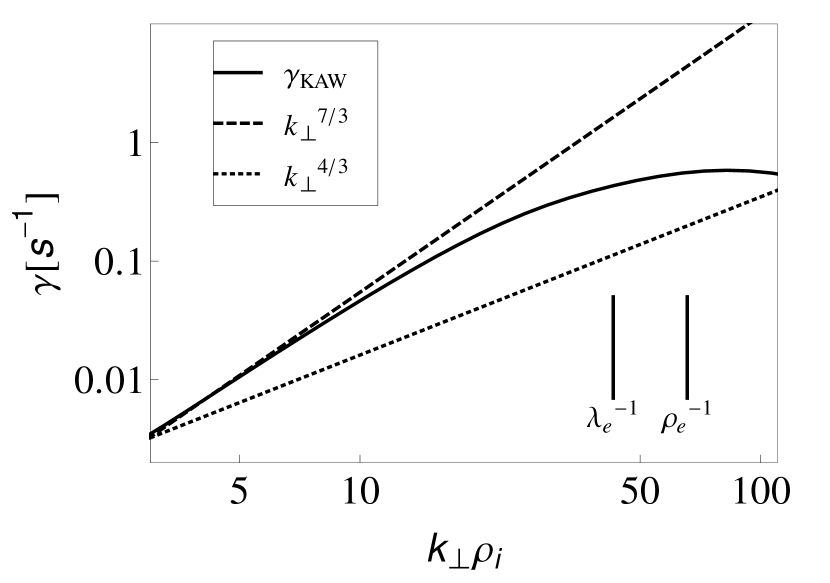
Figure 5: The solid line gives the KAW damping rate from equation (27) for the same parameters as in Figure 2. $k_{\perp}^{4/3}$ and $k_{\perp}^{7/3}$ is shown for comparison. $\lambda_{e}$ and $\rho_{e}$ are marked by the vertical lines.

3 APPLICATION TO THE SOLAR WIND

In this section, we quantitatively compare a model spectrum calculated with hot damping rates and critically balanced wavenumbers with observations in the solar wind, followed by a statistical study to be compared with the statistical study of the set of observations in Alexandrova et al. (2012). The statistical study aims to estimate the dissipation length for varying solar wind conditions. Here we present the first comparison of a dissipation model with a measured magnetic spectrum at electron scales. The blue dots in Figure 6 show observed spectral energy densities by Alexandrova et al. (2009) for $B=15.5$ nT, $n=20$ cm^-3, $T_{i}=61$ eV, $T_{e}=26$ eV, $v_{S}=630$ km/s, and an angle between the mean magnetic field and the solar wind velocity of $\Theta_{BV}=83^{\circ}$. For low frequencies the spectrum follows $\sim f^{-1.7}$ in agreement with Kolmogorov’s law and steepens on ion scales to $\sim f^{-2.8}$. Around the electron scales, the spectrum follows approximately an exponential function (Alexandrova et al., 2009). Our model spectrum is shown in brown for $\kappa=2.7$ for scales below ion scales, where we have applied Taylor’s hypothesis to convert wave vector spectra into frequency spectra using $f=k_{\perp}v_{S}/2\pi$. Apart from the spectral index $\kappa$, and the Kolmogorov constant $C_{K}$, our model equation has no other free parameters. In the ranges of $\kappa=[2.2,2.8]$ and $C_{K}=[1.4,2.1]$, we find through the calculation of the root-mean-square error that the model with $\kappa=2.7$ and $C_{K}=1.4$ describes the data best, but combinations of $\kappa=[2.5,2.7]$ and $C_{K}=[1.4,1.8]$ lead to similar spectral densities within a root-mean-square error difference of 10%. For the choice of the Kolmogorov constant, we follow Biskamp (1993). We discuss the influence of $C_{K}$ on energy spectra in Section 4. Deviations from the theoretically expected value of $\kappa=7/3\approx 2.33$ for KAW (Howes et al., 2006; Schekochihin et al., 2009) may be a result of intermittency effects (Salem et al., 2009; Lion et al., 2016) or superimposition of whistler wave fluctuations (Lacombe et al., 2014). Additionally, damping at electron scales results in spectral indices steeper than $7/3$ due to ’sampling’ effects of one-dimensional spacecraft measurements (von Papen & Saur, 2015). Several different wavevectors contribute to the spectral energy density at a certain spacecraft frequency, so that the sub-ion range is already affected by electron damping. For example, for a field to flow angle of $\Theta_{BV}=90^{\circ}$ this sampling effect steepens a 7/3 spectrum to 2.63 (von Papen & Saur, 2015). In order to take account of these effects, we use a spectral index which fits best to the data. The model spectrum follows in agreement with the observations a power law at the large scales and forms a ’quasi’ exponential decay at the electron scales.

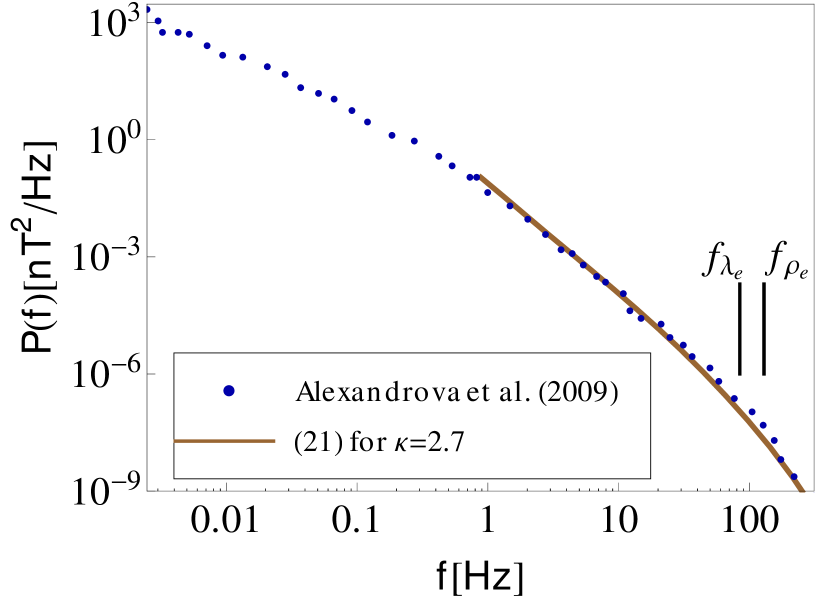
Figure 6: Equation (21) for the same parameters as in Figure 2. Observations from interval 5 in Alexandrova et al. (2009) are shown in blue dots. Vertical lines indicate the electron scales, where $f_{\lambda_{e}}$ corresponds to the Doppler-shifted $\lambda_{e}$, and $f_{\rho_{e}}$ to $\rho_{e}$.

Hence, the observed exponential form of the dissipation range in the observations seems to be compatible with electron Landau damping of kinetic Alfvén waves at least for this set of observations.
For further insight into the spectral behavior for varying parameters, we perform a statistical study with our model similar to the statistical study of 100 observed spectra by Alexandrova et al. (2012). They fit an exponential function with a characteristic dissipation scale $l_{d}$ and with a power law pre-factor

$$P_{A}(k_{\perp})=Ak_{\perp}^{-\alpha}\exp(-k_{\perp}l_{d})$$ (33)

to the solar wind spectra. The study by Alexandrova et al. (2012) finds that the variations of $l_{d}$ due to different solar wind conditions are related to the variations of the electron Larmor radius, $l_{d}\sim 1.35\rho_{e}$, with a high correlation coefficient of 0.7. The correlation between $l_{d}$ and the electron inertial length $\lambda_{e}$ is much weaker with a correlation coefficient of 0.34. The authors assume that the dissipation range in the analyzed set of spectra follows a universal structure of the form of equation (33) for all solar wind parameters. Here we use the same parameter ranges as the observed ones for the magnetic fields, the temperature ratios and the number densities: $B\in[2,20]$ nT, $T_{i}/T_{e}\in[0.5,5]$ and $n_{i}=n_{e}\in[3,60]$ cm^-3. The results of fitting equation (33) to our model through a a least mean square fit are shown in Figures 7 (a) and 7 (b). The red dots show the results for a wide range of ion and electron plasma betas ($\beta_{i}\in[0.1,10]$ and $\beta_{e}\in[0.1,20]$), the black and blue dots show separated results for small ($\beta_{i},\beta_{e}\in[0.1,1]$) and large plasma betas ($\beta_{i}\in[1,10]$ and $\beta_{e}\in[1,20]$), respectively. For every model spectrum, the parameters are chosen randomly within the given parameter ranges using logarithmic distributed values for the temperature ratio and the plasma beta and linear distributed values for the others.

Figure 7: Results of fitting equation (33) to 300 model spectra with hot damping rates. The dissipation length $l_{d}$ is shown as a function of the electron Larmor radius $\rho_{e}$ (a) and of the electron inertial length $\lambda_{e}$ (b). The red dots show the results for $\beta_{i}=[0.1,10]$ and $\beta_{e}=[0.1,20]$, the black and blue dots show separated results for small ($\beta_{i},\beta_{e}=[0.1,1]$) and large plasma betas ($\beta_{i}=[1,10]$ and $\beta_{e}=[1,20]$), respectively.

We find a very high correlation for the electron Larmor radius of 0.98 and a dissipation length $l_{d}\sim 0.9\rho_{e}$, which is similar to the observed value by Alexandrova et al. (2012). Also in agreement with the observational study by Alexandrova et al. (2012), Figure 7 (b) shows a much weaker correlation of 0.41 between the dissipation length $l_{d}$ and the electron inertial length $\lambda_{e}$. This correlation is mainly due to intervals, where $\beta_{e}\approx 1$, which means that the inertial length is comparable to the Larmor radius. Another possible explanation is, that also the inertial length is related to the dissipation scale for some solar wind conditions. For example for small electron plasma betas and low temperatures the electron Larmor radius is very small. In this case, the turbulence might dissipate on an alternative scale, e.g., the electron inertial length, which is reached first by the turbulent cascade. In order to look into this hypothesis, we study the dissipation length separately for small (black line) and large plasma betas (blue line). Indeed, the correlation between the dissipation length and the electron inertial length is higher for small plasma betas with a correlation coefficient of $0.74$ than for large plasma betas with a correlation coefficient of $0.56$. Additionally, the estimated dissipation length in the case of small plasma betas ($l_{d}\sim 1.2\rho_{e}$) is slightly larger than in the large beta case ($l_{d}\sim 0.9\rho_{e}$) suggesting that the energy is dissipated at scales larger than the electron gyroradius.

4 DISCUSSION

Here we discuss a number of assumptions that have been made in the construction of our solar wind dissipation model at electron scales. A range of the Kolmogorov constant $C_{K}=[1.4,2]$ in the solar wind was determined from experimental data and nonlinear simulations (Biskamp, 1993). In this study the constant is taken to be $C_{K}=1.4$ in both the MHD and kinetic regime. However, the ’constant’ may depend on the plasma parameters. For higher $C_{K}$ the argument of the exponential term in equation (21) is larger and therefore the effect of damping is increased in comparison to the nonlinear energy transfer. This variation of the Kolmogorov constant leads to an uncertainty in the magnetic spectra, but without any influence on the general physical description.
Here we use critical balance to obtain the anisotropy of the cascade of energy to smaller scales. This assumption is valid only for strong turbulence. On the contrary, there is no parallel energy cascade in weak turbulence (Sridhar & Goldreich, 1994). However, with increasing $k_{\perp}$ the nonlinear interactions become so strong that the assumption of weakness is no longer valid. Therefore the turbulence is either already strong from the beginning or will eventually become strong for increasing $k_{\perp}$. Yet, our model is not able to handle a changing from strong to weak turbulence when the collisionless damping reduces the amplitudes of the nonlinear interactions to a limit, where weak turbulence should be applied (See Howes et al. (2011) for a weakened cascade model).
The dissipation model presented here is similar to two earlier models, which also contain a nonlinear energy cascade and collisionless damping. Podesta et al. (2010) computed numerically the damping rate from the hot plasma dispersion relation. They conclude that a KAW energy cascade is almost completely dissipated before reaching the electron scales due to strong Landau damping. This would imply that the energy cascade to the electron scales must be supported by wave modes other than the KAW. Howes et al. (2011) argued, that they underestimated the weight of the nonlinear energy cascade in comparison to the dissipation (here described by $C_{K}$), leading to overestimated damping rates. The cascade model in Howes et al. (2008) employs the damping rates obtained from gyrokinetic theory. The authors find in agreement to our results an exponential shaped dissipation range for moderate damping with $\beta_{i}=1$ for $T_{i}/T_{e}=1$. For strong damping($\beta_{i}=0.01$ and $T_{i}/T_{e}=1$) the spectra show sharp cut offs. In Howes et al. (2011) it is assumed that in a model with only local interactions the damping dominates over the energy transfer in the case of strong damping. Therefore they constructed a weakened cascade model with nonlocal interactions. Following Schekochihin et al. (2009), damping can be considered strong if the decay time $1/\gamma$ is shorter or comparable to the wave period $2\pi/\omega_{r}$. Figure 1 shows that damping at $k_{\perp}\rho_{i}=1$ is relatively weak for typical solar wind parameters ($\beta_{i}\gtrsim 1$, $T_{i}/T_{e}\approx[0.5,5]$), thus the nonlocal effects should play a minor role in interpreting the observed energy spectra.
Our dissipation model is a linear model in the sense that it linearly combines the non-linear cascade towards smaller length scales and a process transferring magnetic field energy to particle energy. The mutual feedback of these processes might become stronger at small scales, where the dissipation rates become strong. However, we expect our model to still capture important aspects of the physics around electron scales. In our model we neglect physics on scales significantly beyond the electron scales, e.g., a possible third electrostatic turbulent cascade (Schekochihin et al., 2016).
For mathematical simplicity, we solve the hot plasma dispersion relation assuming Maxwellian distributions of protons and electrons with no temperature anisotropies. Observations of particle distributions show deviations from a Maxwellian due to the weakly collisional nature of the solar wind (Hundhausen et al., 1970; Feldman et al., 1973; Goodrich & Lazarus, 1976). Measured electron distribution functions are composed of an almost Maxwellian and isotropic core for electrons with energy below 50 eV and a highly anisotropic halo representing electrons of higher energy (Briand, 2009). Likewise, observations of proton distribution functions indicate anisotropies between the temperatures parallel and perpendicular to the magnetic field and bump-like deformations at high energy (Marsch et al., 1982). However, due to instabilities limiting the scope of the deformations, the measured deformation of the thermal distribution function is not as strong as expected (Briand, 2009).

5 CONCLUSIONS

We present an analytic dissipation model to describe turbulence at electron scales. It combines the energy transport from large to small scales and the dissipation by collisionless damping of KAWs. The model provides the possibility to analyze and interpret observations of turbulent fluctuations in the dissipation range with in principle arbitrary spectral index in the electron inertial range. The key results of our study are: A direct comparison of our model with observed spectra by Alexandrova et al. (2009, 2012) in the solar wind shows that damping by kinetic Alfvén waves can explain the ’quasi’ exponential spectral structure of the dissipation range at least for the observed solar wind conditions. The dissipation model provides an explanation for the independence of the dissipation scale from the energy cascade rate, which is a remarkable difference compared to hydrodynamic turbulence. This difference is due to the anisotropic nature of the plasma turbulence, i.e., due to a combination of critically balanced turbulence and a dispersion relation proportional to the parallel wavenumber. The critical balance assumption influences the energy cascade in a way, that the more energy is injected at the driving scales, the more effective the damping rate gets. A statistical study of model spectra confirms the high correlation between the dissipation length and the electron Larmor radius, as was reported in Alexandrova et al. (2012). Therefore the Larmor radius may play the role of a dissipation scale in solar wind turbulence. Our dissipation model can easily be applied to other turbulent systems, e.g., planetary magnetospheres for the prediction of spectral energy densities.

Appendix A Hot Plasma Dispersion Relation

A.1 Dielectric Tensor

For a nonrelativistic plasma with Maxwellian distributed electrons and protons with no zero-order drift velocities, the elements of the dielectric tensor can be cast in the form (e.g., Chen, 1984; Stix, 1992)

$$\epsilon_{xx} = 1+\sum_{s}\frac{\omega_{ps}^{2}}{\omega^{2}}\xi_{0s}\sum_{n=-\infty}^{\infty}n^{2}\frac{\Gamma_{n}(\mu_{s})}{\mu_{s}}Z(\xi_{ns})$$ (A1)

$$\epsilon_{yy} = 1+\sum_{s}\frac{\omega_{ps}^{2}}{\omega^{2}}\xi_{0s}\sum_{n=-\infty}^{\infty}\left\{n^{2}\frac{\Gamma_{n}(\mu_{s})}{\mu_{s}}-2\mu_{s}\Gamma_{n}^{\prime}(\mu_{s})\right\}Z(\xi_{ns})$$ (A2)

$$\epsilon_{zz} = 1-\sum_{s}\frac{\omega_{ps}^{2}}{\omega^{2}}\xi_{0s}\sum_{n=-\infty}^{\infty}\xi_{ns}\Gamma_{n}(\mu_{s})Z^{\prime}(\xi_{ns})~{}~{}$$ (A3)

$$\epsilon_{xy} = i\sum_{s}\frac{\omega_{ps}^{2}}{\omega^{2}}\xi_{0s}\sum_{n=-\infty}^{\infty}\Gamma_{n}^{\prime}(\mu_{s})nZ(\xi_{ns})$$ (A4)

$$\epsilon_{xz} = -\sum_{s}\operatorname{sgn}(q_{s})\frac{\omega_{ps}^{2}}{\omega^{2}}\xi_{0s}\sum_{n=-\infty}^{\infty}\frac{1}{\sqrt{2\mu_{s}}}n\Gamma_{n}(\mu_{s})Z^{\prime}(\xi_{ns})$$ (A5)

$$\epsilon_{yz} = i\sum_{s}\operatorname{sgn}(q_{s})\frac{\omega_{ps}^{2}}{\omega^{2}}\xi_{0s}\sum_{n=-\infty}^{\infty}\Gamma_{n}^{\prime}(\mu_{s})Z^{\prime}(\xi_{ns})\sqrt{\frac{\mu_{s}}{2}},$$ (A6)

where $\omega_{ps}=(n_{s}q_{s}^{2}/\epsilon_{0}m_{s})^{1/2}$ is the plasma frequency of species $s$ (with $n_{s}$ the number density, $q_{s}$ the charge, and $m_{s}$ the particle mass), $\Omega_{s}=q_{s}B/m_{s}$ is the gyrofrequency of species $s$ (negative for electrons), $\xi_{ns}=(\omega-n\Omega_{s})/k_{\parallel}v_{s}$, $v_{s}=(2k_{B}T_{s}/m_{s})^{1/2}$ is the thermal speed of species $s$ (with the Boltzmann constant $k_{B}$ and the temperature $T_{s}$), and $\mu_{s}=0.5k_{\perp}^{2}\rho_{s}^{2}$ (with the Larmor radius $\rho_{s}=v_{s}/\Omega_{s}$). The function $Z(\xi)$ is the plasma dispersion function, which was introduced by Fried & Conte (1961). Its derivative is given by $Z^{\prime}(\xi)=-2-2\xi Z(\xi)$. $\Gamma_{n}(\mu_{s})=e^{-\mu_{s}}I_{n}(\mu_{s})$, where $I_{n}\textsection$ is the modified Bessel function of the first kind of order $n$. Note that the derivative of $\Gamma_{n}$ is given by $\Gamma_{n}^{\prime}(\mu_{s})=\left(I_{n}^{\prime}(\mu_{s})-I_{n}(\mu_{s})\right)e^{-\mu_{s}}$.

A.2 Numerical Implementation

If we make no assumptions for the wave frequency and the plasma beta, the full system described by equation (27) needs to be solved numerically to find the wave frequency for given plasma parameters. In contrast to most previous studies, we do not apply the eight-pole approximation (Padé approximation) to evaluate the plasma dispersion function $Z(\xi)$ (see e.g., Rönnmark, 1982) but evaluate the $Z$ function directly in the form

$$Z(\xi)=i\sqrt{\pi}\exp(-\xi^{2})~{}\mathrm{erfc}(\xi)$$ (A7)

with the complementary error function erfc$(\xi)$ (e.g., Abramowitz & Stegun, 1964). In this way, we make sure that the damping rates are evaluated correctly even for heavily damped waves, i.e., $\operatorname{Im}(\omega)>-k_{\parallel}$ or $\operatorname{Im}(\omega)>-\operatorname{Re}(\omega-n\Omega)$ (Rönnmark, 1982).
A two-dimensional Newton’s method root search in the complex frequency plane is used here to find the solution of equation (27). To ensure accurate results for high perpendicular wavenumbers, the number of sum elements that are kept is about the same as $k_{\perp}\rho_{i}$ (Howes et al., 2006). We implemented an iterative root search to track the required wave mode from small wavenumbers to large wavenumbers. An initial guess of the frequency is set at a given initial wavenumber (e.g., MHD Alfvén wave frequency to track the kinetic Alfvén wave). At neighboring wavenumbers, the solution is then found by using the previously obtained frequency as an initial guess.

References

- Abramowitz & Stegun (1964) Abramowitz, M., & Stegun, I. A. 1964, Handbook of Mathematical Functions: with Formulas, Graphs, and Mathematical Tables (New York: Dover Publications, Inc.)
- Alexandrova et al. (2008) Alexandrova, O., Carbone, V., Veltri, P., & Sorriso-Valvo, L. 2008, ApJ, 674, 1153
- Alexandrova et al. (2012) Alexandrova, O., Lacombe, C., Mangeney, A., Grappin, R., & Maksimovic, M. 2012, ApJ, 760, 121
- Alexandrova et al. (2009) Alexandrova, O., Saur, J., Lacombe, C., et al. 2009, PhRvL, 103, 165003
- Bagenal & Delamere (2011) Bagenal, F., & Delamere, P. A. 2011, JGRA, 116, A05209
- Bale et al. (2005) Bale, S. D., Kellogg, P. J., Mozer, F. S., Horbury, T. S., & Reme, H. 2005, PhRvL, 94, 215002
- Barnes (1979) Barnes, A. 1979, Space Plasma Physics. The Study of Solar-System Plasmas, 2, 257
- Bieber et al. (1993) Bieber, J. W., Chen, J., Matthaeus, W. H., Smith, C. W., Pomerantz, M. A. 1993, JGRA, 98, 3585
- Bieber et al. (1996) Bieber, J. W., Wanner, W., Matthaeus, W. H. 1996, JGR, 101, 2511
- Biskamp (1993) Biskamp D. 1993, Nonlinear Magnetohydrodynamics (Cambridge: Cambridge Univ. Press)
- Boldyrev et al. (2013) Boldyrev, S., Horaites, K., Xia, Q., & Perez, J. C. 2013, ApJ, 777, 41
- Briand (2009) Briand, C. 2009, NPGeo, 16, 319
- Bruno & Carbone (2013) Bruno, R., & Carbone, V. 2013, LRSP, 10, 2
- Bruno & Trenchi (2014) Bruno, R., & Trenchi, L. 2014, ApJL, 787, L24
- Chen et al. (2013) Chen, C. H. K., Boldyrev, S., Xia, Q., & Perez, J. C. 2013, PhRvL, 110, 225002
- Chen et al. (2014) Chen, C. H. K., Leung, L., Boldyrev, S., Maruca, B. A., & Bale, S. D. 2014, GeoRL, 41, 8081
- Chen et al. (2010) Chen, C. H. K., Horbury, T. S., Schekochihin, A. A., et al. 2010, PhRvL, 104, 255002
- Chen (1984) Chen, F. F. 1974, Introduction to Plasma Physics and Controlled Fusion, Volume 1: Plasma Physics (New York: Springer US)
- Cho & Lazarian (2004) Cho, J., Lazarian, A. 2004, ApJ, 615, L41
- Corrsin (1964) Corrsin, S. 1964, PhFl, 7, 1156
- Denskat et al. (1983) Denskat, K. U., Beinroth, H. J., & Neubauer, F. M. 1983, JGZG, 54, 60
- Drake (2006) Drake, R. P. 2006, High-Energy-Density Physics, ed. L. Davison, Y. Horie (Berlin Heidelberg: Springer)
- Farmer & Goldreich (2004) Farmer, A. J., & Goldreich, P. 2004, ApJ, 604, 671
- Feldman et al. (1973) Feldman, W. C., Asbridge, J. R., Bame, S. J., & Montgomery, M. D. 1973, JGR, 78, 2017
- Fried & Conte (1961) Fried, B. D., Conte, S. D. 1961, The Plasma Dispersion Function (New York: Academic Press)
- Frisch (1995) Frisch, U. 1995, Turbulence - the Legacy of A. N. Kolmogorov (Cambridge: Cambridge Univ. Press)
- Gary & Nishimura (2004) Gary, S. P., Nishimura, K. 2004, JGRA, 109, A02109
- Gary & Smith (2009) Gary, S. P., & Smith, C. W. 2009, JGRA, 114, A12105
- Goldreich & Sridhar (1995) Goldreich, P., & Sridhar, S. 1995, ApJ, 438, 763
- Goodrich & Lazarus (1976) Goodrich, C. C., & Lazarus, A. J. 1976, JGR, 81, 2750.
- He et al. (2013) He, J., Tu, C., Marsch, E., Bourouaine, S., & Pei, Z. 2013, ApJ, 773, 72
- Horbury et al. (1996) Horbury, T. S., Balogh, A., Forsyth, R. J., & Smith, E. J. 1996, A&A, 316, 333
- Horbury et al. (2008) Horbury, T. S., Forman, M., & Oughton, S. 2008, PhRvL, 101, 175005
- Horbury et al. (2012) Horbury, T. S., Wicks, R. T., & Chen, C. H. K. 2012, SSRv, 172, 325
- Howes (2015) Howes, G. G. 2015, RSPTA, 373, 20140145
- Howes et al. (2006) Howes, G. G., Cowley, S. C., Dorland, W., et al. 2006, ApJ, 651, 590
- Howes et al. (2008) Howes, G. G., Cowley, S. C., Dorland, W., et al. 2008, JGRA, 113, A05103
- Howes et al. (2011) Howes, G. G., TenBarge, J. M., & Dorland, W. 2011, PhPl, 18, 102305
- Hundhausen et al. (1970) Hundhausen, A. J., Bame, S. J., Asbridge, J. R., & Sydoriak, S. J. 1970, JGR, 75, 4643
- Jokipii (1966) Jokipii, J. R. 1966, ApJ, 146, 480
- Kiyani et al. (2009) Kiyani, K. H., Chapman, S. C., Khotyaintsev, Y. V., Dunlop, M. W., & Sahraoui, F. 2009, PhRvL, 103, 075006
- Kolmogorov (1941) Kolmogorov, A. N. 1941, DoSSR, 30, 299 (English translation: 1991, RSPSA, 434, 9)
- Kovasznay (1948) Kovasznay, L. S. G. 1948, PhRv, 73, 1115
- Lacombe et al. (2014) Lacombe, C., Alexandrova, O., Matteini, L., et al. 2014, ApJ, 796, 5
- Leamon et al. (1998) Leamon, R. J., Smith, C. W., Ness, N. F., Matthaeus, W. H., & Wong, H. K. 1998, JGR, 103, 4775
- Leamon et al. (1999) Leamon, R. J., Smith, C. W., Ness, N. F., & Wong, H. K. 1999, JGR, 104, 22331
- Li et al. (2011) Li, G., Miao, B., Hu, Q., & Qin, G. 2011, PhRvL, 106, 125001
- Lion et al. (2016) Lion, S., Alexandrova, O., & Zaslavsky, A. 2016, ApJ, 824, 47
- Lysak & Lotko (1996) Lysak, R. L., & Lotko, W. 1996, JGR, 101, 5085
- Marsch et al. (1982) Marsch, E., Mühlhäuser, K.-H., Schwenn, R., et al. 1982, JGRA, 87, 52
- Matthaeus et al. (1990) Matthaeus, W. H., Goldstein, M. L., & Roberts, D. A. 1990, JGRA, 95, 20673
- Matthaeus et al. (1982) Matthaeus, W. H., Goldstein, M. L., & Smith, C. 1982, PhRvL, 48, 1256
- Narita et al. (2010) Narita, Y., Glassmeier, K.-H., Sahraoui, F., & Goldstein, M. L. 2010, PhRvL, 104, 171101
- Narita et al. (2011) Narita, Y., Gary, S. P., Saito, S., Glassmeier, K.-H., & Motschmann, U. 2011, GeoRL, 38, L05101
- Narita & Marsch (2015) Narita, Y. & Marsch, E. 2015, ApJ, 805, 24
- Narita (2015) Narita, Y. 2015, AnGeo, 33, 1413
- Pao (1965) Pao, Y.-H. 1965, PhFl, 8, 1063
- Podesta (2009) Podesta, J. J. 2009, ApJ, 2, 986
- Podesta et al. (2010) Podesta, J. J., Borovsky, J. E., Gary, S. P. 2010, ApJ, 712, 685.
- Richardson et al. (1995) Richardson, J. D., Paularena, K. I., Lazarus, A. J., & Belcher, J. W. 1995, GeoRL, 22, 325
- Roberts et al. (2013) Roberts, O. W., Li, X., & Li, B. 2013, ApJ, 769, 58
- Rönnmark (1982) Rönnmark, K. 1982, Kiruna Geophys. Inst. Rep, 179, 56
- Sahraoui et al. (2012) Sahraoui, F., Belmont, G., & Goldstein, M. L. 2012, ApJ, 748, 100
- Sahraoui et al. (2010) Sahraoui, F., Goldstein, M. L., Belmont, G., Canu, P., & Rezeau, L. 2010, PhRvL, 105, 131101
- Sahraoui et al. (2009) Sahraoui, F., Goldstein, M. L., Robert, P., & Khotyaintsev, Y. V. 2009, PhRvL, 102, 231102
- Sahraoui et al. (2013) Sahraoui, F., Huang, S. Y., Belmont, G., et al. 2013, ApJ, 777, 15
- Salem et al. (2012) Salem, C. S., Howes, G. G., Sundkvist, D., et al. 2012, ApJ, 745, L9
- Salem et al. (2009) Salem, C., Mageney, A., Bale, S. D., & Veltri, P. 2009, ApJ, 702, 537
- Saur (2004) Saur, J. 2004, ApJ, 602, L137
- Schekochihin et al. (2009) Schekochihin, A. A., Cowley, S. C., Dorland, W., et al. 2009, ApJS, 182, 310
- Schekochihin et al. (2016) Schekochihin, A. A., Parker, J. T., Highcock, E. G., et al. 2016, JPlPh, 82, 905820212
- Smith et al. (2006) Smith, C. W., Hamilton, K., Vasquez, B. J., & Leamon, R. J. 2006, ApJ, 645, L85
- Smith et al. (2012) Smith, C. W., Vasquez, B. J., & Hollweg, J. V. 2012, ApJ, 745, 8
- Sridhar & Goldreich (1994) Sridhar, S., & Goldreich, P. 1994, ApJ, 432, 612
- Stix (1992) Stix, T. H. 1992, Waves in Plasmas (New York: AIP)
- TenBarge & Howes (2012) TenBarge, J. M., & Howes, G. G. 2012, PhPl, 19, 055901
- von Papen et al. (2014) von Papen, M., Saur, J., Alexandrova, O. 2014, JGRA, 119, 2797
- von Papen & Saur (2015) von Papen, M., Saur, J. 2015, ApJ, 806, 116
- Wang et al. (2014) Wang, X., Tu, C., He, J., Marsch, E., & Wang, L. 2014, ApJ, 783, L9
- Zhao et al. (2013) Zhao, J. S., Wu, D. J., & Lu, J. Y. 2013, ApJ, 767, 109