On the Cohomology of Contextuality

Abstract

Recent work by Abramsky and Brandenburger used sheaf theory to give a mathematical formulation of non-locality and contextuality. By adopting this viewpoint, it has been possible to define cohomological obstructions to the existence of global sections. In the present work, we illustrate new insights into different aspects of this theory. We shed light on the power of detection of the cohomological obstruction by showing that it is not a complete invariant for strong contextuality even under symmetry and connectedness restrictions on the measurement cover, disproving a previous conjecture. We generalise obstructions to higher cohomology groups and show that they give rise to a refinement of the notion of cohomological contextuality: different “levels” of contextuality are organised in a hierarchy of logical implications. Finally, we present an alternative description of the first cohomology group in terms of torsors, resulting in a new interpretation of the cohomological obstructions.

1 Introduction

Contextuality is one of the most fundamental and peculiar features of quantum mechanics. Inspired by classic no-go theorems by Bell [10] and Kochen-Specker [18], the development of quantum information has been increasingly influenced by the study of this highly non-classical phenomenon. Recent work by Howard et al. has even suggested that it actually represents the source of the power of quantum computing [17]. The sheaf-theoretic description of non-locality and contextuality introduced in [4] has proved that contextuality is in fact a general mathematical property that goes beyond quantum physics and pervades various domains (e.g. relational databases [2] and constraint satisfaction [5]).

This rigorous mathematical formulation has allowed the application of powerful methods of sheaf cohomology to the study of the topological structure of contextuality [3, 6]. Central to this approach is the notion of cohomological obstruction to the existence of global sections, i.e. elements of the first Čech cohomology group that provide a sufficient (but not necessary) condition for the contextuality of empirical models. Although cohomology has been proved to correctly detect contextuality in various well-studied empirical models such as PR boxes [26], GHZ states [13, 14, 21], the Peres-Mermin “magic” square [23, 22, 25] and the whole class of models admitting “All-vs-Nothing” arguments [3] , there is evidence of a restricted number of false positives (e.g. the Hardy model [16]).

In the present paper, we illustrate new insights into the properties of cohomological obstructions with the ultimate goal of understanding how such false positives arise. In particular, we aim to give an answer to some of the open questions left by [6]: “Is the cohomological obstruction a full invariant for strong contextuality under suitable restrictions on the measurement scenario?”; “Can higher cohomology groups be used for the study of contextuality?”; “Is there a concrete way of describing cohomological obstructions?”.

We briefly outline our results:

• We disprove Conjecture 8.1 of [6] by providing an explicit example of a strongly contextual but cohomologically non-contextual empirical model defined on a simple $(2,2,4)$ Bell-type scenario which verifies any reasonably strong form of connectedness and symmetry condition.

• We generalise cohomological obstructions to higher cohomology groups. It turns out that this procedure can be done in a natural way only in odd dimensions. We obtain a refinement of the notion of cohomological contextuality: for each $q\geq 0$, we say that a model is $q$-cohomologically contextual if the $q$-th obstruction does not vanish.

• We show that higher obstructions are organised in a precise hierarchy of logical implications. We also prove that, unfortunately, this result cannot be used in the study of contextuality in no-signalling empirical models. Despite this fact, higher obstructions could potentially be used to study signalling properties.

• We give a new description of the first cohomology group (thus, in particular, of the cohomology obstructions) using torsors relative to a presheaf.

The paper is organised as follows. We summarise the sheaf viewpoint from [4] in Section 2, and recall the main definitions concerning sheaf cohomology in Section 3. Section 4 features the counterexample to Conjecture 8.1 of [6]. We generalise cohomological obstructions to higher cohomology groups in Section 5. Finally, in Section 6, we present torsors relative to a presheaf, and their relation to the first sheaf cohomology group.

2 The sheaf-theoretic framework

In this section we recall the main definitions of the sheaf-theoretic approach to non-locality and contextuality [4].

We start by considering a finite discrete space $X$, which can be seen as a set of measurement labels. We define a measurement cover as an antichain $\mathcal{M}=\{C_{i}\}_{i\in I}$ that satisfies $\bigcup_{i\in I}C_{i}=X$. This family contains the maximal sets of measurements that can be jointly performed, called measurement contexts. The set $X$, together with the cover $\mathcal{M}$ and a fixed finite set of outcomes $O$, constitute the measurement scenario $\langle X,\mathcal{M},O\rangle$, which represents the basic setting of the experiment we aim to study.

We consider $X$ as a discrete topological space and define the sheaf of events

$$\mathcal{E}:\textbf{Open}(X)^{op}=\mathcal{P}(X)^{op}\rightarrow\textbf{Set},$$

where $\mathcal{E}(U):=O^{U}$ for each subset $U\subseteq X$, and restriction maps coincide with function restriction: for $U\subseteq U^{\prime}\subseteq X$, we have

$$\rho_{U}^{U^{\prime}}:=\mathcal{E}(U\subseteq U^{\prime}):O^{U^{\prime}}\rightarrow O^{U}::s\mapsto s\mid_{U}.$$

Each $s\in\mathcal{E}(U)$ is called a section, in particular $g\in\mathcal{E}(X)$ is a global section.

A probabilistic empirical model $e$ is a compatible family $\{e_{C}\}_{C\in\mathcal{M}}$, where $e_{C}$ is a probability distribution over $\mathcal{E}(C)$. In this paper we will only consider possibilistic empirical models, i.e. the ones generated by the support of a probabilistic model.

Such models can be defined as subpresheaves $\mathcal{S}$ of $\mathcal{E}$ that verify the following properties:

1. $\mathcal{S}(C)\neq\emptyset$ for all $C\in\mathcal{M}$

2. $\mathcal{S}$ is flasque beneath the cover, i.e. the map $\mathcal{S}(U\subseteq U^{\prime})$ is surjective whenever $U\subseteq U^{\prime}\subseteq C$ for some $C\in\mathcal{M}$.

3. Every family $\{s_{C}\in\mathcal{S}(C)\}_{C\in\mathcal{M}}$ which is compatible (i.e. such that $s_{C}\mid_{C\cap C^{\prime}}=s_{C^{\prime}}\mid_{C\cap C^{\prime}}$ for all $C,C^{\prime}\in\mathcal{M}$) induces a global section in $\mathcal{S}(X)$. Note that this global section is unique since $\mathcal{S}$ is a subpresheaf of the sheaf $\mathcal{E}$.

These conditions state that $\mathcal{S}$ is completely determined by its values $\mathcal{S}(C)$ at each context $C\in\mathcal{M}$: values $\mathcal{S}(U)$ below the cover are fixed by flaccidity, and values for subsets $U$ above the cover are determined by condition 3. Flaccidity beneath the cover can also be interpreted as a possibilistic version of no-signalling.

Contextuality of an empirical model $\mathcal{S}$ on a measurement scenario $\langle X,\mathcal{M},O\rangle$ can be characterised as follows

• Given a context $C\in\mathcal{M}$ and a section $s\in\mathcal{S}(C)$, $\mathcal{S}$ is logically contextual at $s$, or $\mbox{LC}(\mathcal{S},s)$, if $s$ is not a member of any compatible family. We say that $\mathcal{S}$ is logically contextual, or $\mbox{LC}(\mathcal{S})$, if $\mbox{LC}(\mathcal{S},s)$ for some possible section $s$.

• $\mathcal{S}$ is strongly contextual, or $\mbox{SC}(\mathcal{S})$, if $\mbox{LC}(\mathcal{S},s)$ for all $s$. In other words there is no global section ($\mathcal{S}(X)=\emptyset$).

2.1 Bundle diagrams

The structure of the measurement cover can equivalently be described as an abstract simplicial complex having measurements as vertices [8, 9]. A set of vertices forms a face whenever the corresponding measurements can be jointly performed, hence contexts correspond to facets of the complex. This viewpoint allows us to graphically represent simple possibilistic empirical models as bundle diagrams. In figure 1 we have depicted the bundle diagram of a simple $(2,2,2)$ Bell-type scenario involving two agents Alice and Bob who can choose between two binary measurements each ($a_{1},a_{2}$ for Alice and $b_{1},b_{2}$ for Bob).

Figure 1: A $(2,2,2)$ Bell-type scenario. The section $(a_{1},b_{1})\mapsto(1,1)$ is represented in the centre. On the right, the global section $(a_{1},b_{1},a_{2},b_{2})\mapsto(1,1,0,0)$

The measurement simplicial complex lies at the base of the bundle, and above each vertex is a fibre of the values that can be assigned to each measurement ($0$ or $1$ in this case). A possible section is represented by an edge connecting the outcomes involved above the corresponding context as in the central diagram of the figure. No-signalling corresponds to the property that each edge above a context can be extended to at least one edge above each adjacent context. A global section is represented by a closed path traversing all the fibers exactly once as shown on the right-hand side of Figure 1.

Using this handy representation, we can have an immediate feedback on the contextuality of empirical models. As an example, consider the Hardy model [16, 15] and the Popescu-Rohrlich (PR) box model [26] represented in Figure 2.

$A$	$B$	$(0,0)$	$(1,0)$	$(0,1)$	$(1,1)$
$a_{1}$	$b_{1}$	$1$	$1$	$1$	$1$
$a_{1}$	$b_{2}$	$0$	$1$	$1$	$1$
$a_{2}$	$b_{1}$	$0$	$1$	$1$	$1$
$a_{2}$	$b_{2}$	$1$	$1$	$1$	$0$

(a) Hardy model

$A$	$B$	$(0,0)$	$(1,0)$	$(0,1)$	$(1,1)$
$a_{1}$	$b_{1}$	$1$	$0$	$0$	$1$
$a_{1}$	$b_{2}$	$1$	$0$	$0$	$1$
$a_{2}$	$b_{1}$	$1$	$0$	$0$	$1$
$a_{2}$	$b_{2}$	$0$	$1$	$1$	$0$

(b) PR-Box model

We can clearly see that the section $(a_{1},b_{1})\mapsto(0,0)$ in the Hardy bundle, marked in red, is not part of any compatible family, hence the model is logically contextual. However, it is not strongly contextual since there is a global section $(a_{,}b_{1},a_{2},b_{2})\mapsto(1,1,0,0)$ (marked in blue). On the other hand, all the sections in the PR-Box bundle are not part of any compatible family, which means that the model is strongly contextual.

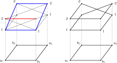
Figure 2: The Hardy model and the PR-Box model as bundle diagrams.

3 Sheaf cohomology

We recall the main results of [3, 6] concerning cohomological obstructions to the existence of global sections.

Consider a measurement scenario $\langle X,\mathcal{M},O\rangle$ and an empirical model $\mathcal{S}$ defined on it. We define a presheaf of abelian groups $\mathcal{F}:\mathcal{P}(X)^{op}\rightarrow\textbf{AbGrp}$ that represents $\mathcal{S}$. Explicitly, this means that $\mathcal{F}$ verifies conditions 1, 2 and 3, and that there is an injection $i:\mathcal{S}\hookrightarrow\mathcal{F}$ such that $i_{C}(s_{C})\neq 0\in\mathcal{F}(C)$ for all $C\in\mathcal{M}$ and for each $s_{C}\in\mathcal{S}(C)$. Typically, $\mathcal{F}:=F_{\mathbb{Z}}\mathcal{S}$ is used, where $F_{\mathbb{Z}}:\textbf{Set}\rightarrow\textbf{AbGrp}$ is the functor that assigns to a set $X$ the free abelian group $F_{\mathbb{Z}}(X)$ generated by it.

A $q$-simplex of the nerve of $\mathcal{M}$ is a tuple $\sigma=(C_{0},\dots,C_{q})$ of elements of $\mathcal{M}$ such that $|\sigma|:=\cap_{i=0}^{q}C_{i}\neq\emptyset$. The set of $q$-simplices is denoted by $\mathcal{N}(\mathcal{M})^{q}$. The nerve $\mathcal{N}(\mathcal{M})$ is the abstract simplicial complex generated by all the $\mathcal{N}(\mathcal{M})^{q}$s. For all $q\geq 0$ and each $0\leq j\leq q$, we can define the maps $\partial_{j}:\mathcal{N}(\mathcal{M})^{q+1}\rightarrow\mathcal{N}(\mathcal{M})^{q}$ by the expression

$$\partial_{j}(C_{0},\dots,C_{q+1}):=(C_{0},\dots,C_{j-1},\hat{C_{j}},C_{j+1},\dots,C_{q+1}).$$

This allows us to define the augmented Čech cochain complex

$$0\xrightarrow{\leavevmode\nobreak\ 0\leavevmode\nobreak\ }C^{0}(\mathcal{M},\mathcal{F})\xrightarrow{\delta^{0}}C^{1}(\mathcal{M},\mathcal{F})\xrightarrow{\delta^{1}}\dots$$

where, for all $q\geq 0$,

$$C^{q}(\mathcal{M},\mathcal{F}):=\bigoplus_{\sigma\in\mathcal{N}(\mathcal{M})^{q}}\mathcal{F}(|\sigma|)$$

is the abelian group of $q$-cochains, and $\delta^{q}:C^{q}(\mathcal{M},\mathcal{F})\rightarrow C^{q+1}(\mathcal{M},\mathcal{F})$ defined by

$$\delta^{q}(\omega)(\sigma):=\sum_{j=0}^{q+1}(-1)^{j}\rho_{|\sigma|}^{|\partial_{j}\sigma|}(\omega(\partial_{j}\sigma))\leavevmode\nobreak\ \leavevmode\nobreak\ \forall\omega\in C^{q}(\mathcal{M},\mathcal{F}),\leavevmode\nobreak\ \forall\sigma\in\mathcal{N}(\mathcal{M})^{q}$$

is the $q$-th coboundary map, where $\rho_{|\sigma|}^{|\partial_{j}\sigma|}$ denotes the restriction homomorphism $\mathcal{F}(|\sigma|\subseteq|\partial_{j}\sigma|)$. Čech cohomology $\check{H}^{\ast}(\mathcal{M},\mathcal{F})$ is defined as the cohomology of this augmented cochain complex.

We assume that $\mathcal{M}$ is a connected cover, i.e. given $C,C^{\prime}\in\mathcal{M}$ there exists a sequence of contexts $C=C_{0},C_{1},\dots,C_{n}=C^{\prime}$ such that $C_{i}\cap C_{i+1}\neq\emptyset$. Thanks to this assumption, cocycles in $Z^{0}(\mathcal{M},\mathcal{F})\cong\check{H}^{0}(\mathcal{M},\mathcal{F})$ correspond to compatible families $\{r_{C}\in\mathcal{F}(C)\}_{C\in\mathcal{M}}$ (i.e. such that $r_{C}\mid_{C\cap C^{\prime}}=r_{C^{\prime}}\mid_{C\cap C^{\prime}}$ for all $C,C^{\prime}\in\mathcal{M}$).

In order to study the extendability of a local section at a fixed context $C_{0}\in\mathcal{M}$, we shall define the relative cohomology of $\mathcal{F}$. We introduce two auxiliary presheaves. Firstly

$$\mathcal{F}\mid_{C_{0}}:\textbf{Open}(X)^{op}\rightarrow\textbf{AbGrp}::U\mapsto\mathcal{F}(U\cap C_{0}).$$

The restriction to $C_{0}$ yields an obvious morphism of sheaves $p^{C_{0}}:\mathcal{F}\Rightarrow\mathcal{F}\mid_{C_{0}}$ defined by

$$p^{C_{0}}_{U}:\mathcal{F}(U)\rightarrow\mathcal{F}\mid_{C_{0}}(U)::r\mapsto r\mid_{C_{0}\cap U}.$$

Notice that each $p^{C_{0}}_{U}$ is surjective since $\mathcal{F}$ is flasque beneath the cover and $U\cap C_{0}\subseteq C_{0}\in\mathcal{M}$. The second auxiliary functor is defined by $\mathcal{F}_{\tilde{C}_{0}}(U):=\ker(p_{U}^{C_{0}})$. Thus, we have an exact sequence of presheaves

$$\textbf{0}\Longrightarrow\mathcal{F}_{\tilde{C}_{0}}\Longrightarrow\mathcal{F}\xRightarrow{\leavevmode\nobreak\ p^{C_{0}}}\mathcal{F}\mid_{C_{0}},$$ (1)

which can be lifted to cochains to

$$0\longrightarrow C^{0}(\mathcal{M},\mathcal{F}_{\tilde{C}_{0}})\xhookrightarrow{\leavevmode\nobreak\ \leavevmode\nobreak\ \leavevmode\nobreak\ \leavevmode\nobreak\ \leavevmode\nobreak\ \leavevmode\nobreak\ \leavevmode\nobreak\ }C^{0}(\mathcal{M},\mathcal{F})\xrightarrow{\bigoplus_{C}p_{C}^{C_{0}}}C^{0}(\mathcal{F},\mathcal{F}\mid_{C_{0}}),\longrightarrow 0,$$

where exactness on the right is given by surjectivity of all the $p_{C}^{C_{0}}$. The map $\delta^{0}$ can be correstricted to a map $\tilde{\delta^{0}}:=\delta^{0}\mid^{Z^{1}(\mathcal{M},\mathcal{F})}$ whose kernel is $Z^{0}(\mathcal{M},\mathcal{F})\cong\check{H}^{0}(\mathcal{M},\mathcal{F})$ and whose cokernel is isomorphic to $\check{H}^{1}(\mathcal{M},\mathcal{F})$ (the same procedure can be applied to $\mathcal{F}\mid_{C_{0}}$ and $\mathcal{F}_{\tilde{C}_{0}}$). Therefore, by applying the snake lemma to

we obtain an exact sequence

where the “snake” homomorphism $\gamma_{C_{0}}$ is called the connecting homomorphism relative to the context $C_{0}$. We have $\mathcal{F}(C_{0})\cong\check{H}^{0}(\mathcal{M},\mathcal{F}\mid_{C_{0}})$ via the isomorphism

$$\psi^{0}:\mathcal{F}(C_{0})\rightarrow Z^{0}(\mathcal{M},\mathcal{F}\mid_{C_{0}})::r_{C_{0}}\mapsto(r_{C_{0}}\mid_{C_{0}\cap C})_{C\in\mathcal{M}}.$$ (2)

Thus, given an element $r_{0}\in\mathcal{F}(C_{0})$, it makes sense to define the cohomological obstruction of $r_{0}$ as the element $\gamma_{C_{0}}(r_{0})\in\check{H}^{1}(\mathcal{M},\mathcal{F}_{\tilde{C}_{0}})$.

We have the following key result from [6]:

Proposition 3.1.

Let $\mathcal{M}$ be a connected cover, $C_{0}\in\mathcal{M}$ and $r_{0}\in\mathcal{F}(C_{0})$. Then, $\gamma_{C_{0}}(r_{0})=0$ if and only if there exists a compatible family $\{r_{C}\in\mathcal{F}(C)\}_{C\in\mathcal{M}}$ such that $r_{C_{0}}=r_{0}$.

Given an empirical model $\mathcal{S}$ and a local section $s_{0}\in\mathcal{S}(C_{0})$, we define the following notions

• $\mathcal{S}$ is cohomologically logically contextual at $s_{0}$, or $\mbox{CLC}(\mathcal{S},s_{0})$, if $\gamma_{C_{0}}(s_{0})\neq 0$. We say that $\mathcal{S}$ is cohomologically logically contextual, or $\mbox{CLC}(\mathcal{S})$, if $\mbox{CLC}(\mathcal{S},s)$ for some section $s$.

• $\mathcal{S}$ is cohomologically strongly contextual, or $\mbox{\mbox{CSC}}(\mathcal{S})$, if $\mbox{CLC}(\mathcal{S},s)$ for all sections $s$.

The main result of [6] provides a sufficient condition for an empirical model to be contextual:

Theorem 3.2.

Let $\mathcal{S}$ be an empirical model. We have $\rm{CLC}(\mathcal{S})\Rightarrow\mbox{LC}(\mathcal{S})$ and $\mbox{\mbox{CSC}}(\mathcal{S})\Rightarrow\mbox{SC}(\mathcal{S})$.

However, it is sufficient to consider the Hardy model to show that this condition is not necessary [6]. Bundle diagrams can be used again to understand how such false positives arise. As an example, consider the diagram of the Hardy model in Figure 3.

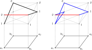
Figure 3: The Hardy model is LC but not CLC

On the left-hand side we graphically show that the red section $s:=(a_{1},b_{1})\mapsto(0,0)$ cannot be extended to a compatible family, proving local contextuality at $s$. However, when considering the presehaf of abelian groups $\mathcal{F}:=F_{\mathbb{Z}}\mathcal{S}$ needed to define cohomological obstructions, we are allowed to take formal linear combinations of sections over the same context. Thus, it is possible to obtain closed paths like the one in blue on the right-hand side of Figure 3, which is explicitly defined by

$$\{s,(a_{2},b_{1})\mapsto(1,0),(a_{2},b_{2})\mapsto(1,0),[(a_{1},b_{2})\mapsto(1,0)]-[(a_{1},b_{2})\mapsto(1,1)]+[(a_{1},b_{2})\mapsto(0,1)]\},$$

and represents a compatible family for $\mathcal{F}$. The existence of such a closed path shows why cohomology cannot detect contextuality in this case.

4 A false positive for strong contextuality

In [6], it is brought to attention that, although cohomology can fail to detect logical contextuality as in the case of the Hardy model, it is rather difficult to construct a strongly contextual false positive. Indeed, cohomology is able to detect the strong contextuality of a variety of well-known models, including GHZ states [13, 14, 21], PR Boxes [26], the Peres-Mermin “magic” square [23, 22, 25], all $\neg GCD$ models [6], and the whole class of models admitting All-vs-Nothing arguments [3]. The only known example of a strongly contextual false positive is the Kochen-Specker model [18, 20] for the cover

$$\{A,B,C\},\{B,D,E\},\{C,D,E\},\{A,D,F\},\{A,E,G\},$$

which “does not satisfy any reasonable criterion for symmetry, nor does it satisfy any strong form of connectedness” and where “the existence of measurements belonging to a single context, namely $F$ and $G$, seems to be crucial” [6]. Due to these limitations, the following conjecture was made:

Conjecture 4.1 (Conjecture 8.1 of [6]).

Under suitable assumptions of symmetry and connectedness of the cover, the cohomology obstruction is a complete invariant for strong contextuality.

In Figure 4, we introduce a counterexample to this conjecture.

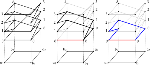
Figure 4: A $\mbox{SC}\wedge\neg\mbox{CLC}$ model over a $(2,2,4)$ scenario

The bundle diagram on the left-hand side represents an empirical model $\mathcal{S}$ (the explicit definition can be found in Appendix A) on a $(2,2,4)$ Bell-type scenario. Note that this measurement scenario is extremely simple and verifies any reasonably strong form of symmetry and connectedness. By carefully analysing the picture, one verifies that none of the sections can be extended to a compatible family of $\mathcal{S}$ (i.e. a closed path containing one and only one section per context), but each one of them is contained in a compatible family of $\mathcal{F}:=F_{\mathbb{Z}}\mathcal{S}$, namely a closed path similar to the one generating the false positive for the Hardy model (Figure 3). As an example, we show this feature by considering the section $s_{0}:=(a_{1},b_{1})\mapsto(0,0)$: from the central diagram of Figure 4 it appears clear that this section is non-extendable to a compatible family of $\mathcal{S}$, while the diagram on the right-hand side shows that $s_{0}$ is part of a compatible family for $\mathcal{F}$, explicitly defined as

$$\{s_{0},(a_{2},b_{1})\mapsto(0,0),(a_{2},b_{2})\mapsto(0,1),[(a_{1},b_{1})\mapsto(1,1)]-[(a_{1},b_{1})\mapsto(1,0)]+[(a_{1},b_{1})\mapsto(0,0)]\}.$$

We conclude that this model is strongly contextual but not cohomologically contextual (not even cohomologically logically contextual), essentially disproving Conjecture 8.1 of [6].

5 Higher cohomology groups

The theory developed so far involves only the first Čech cohomology group, which contains the obstructions. The existence of badly behaved false positives like the one presented in the previous section motivates a deeper inspection of the higher cohomology groups in search of information on how such extreme cases arise. We will introduce here a generalisation of cohomology obstructions to higher-dimensional cohomology groups.

Let $\mathcal{F}$ be an abelian presheaf representing an empirical model $\mathcal{S}$ on a scenario $\langle X,\mathcal{M},O\rangle$ (e.g. $\mathcal{F}:=F_{\mathbb{Z}}\mathcal{S}$). Let $q\geq 0$ be an integer and fix a context $C_{0}\in\mathcal{M}$. To each section $s_{0}\in\mathcal{F}(C_{0})$ we associate a $q$-relative cochain $c_{s_{0}}^{q}\in C^{q}(\mathcal{M},\mathcal{F}\mid_{C_{0}})$ defined by

$$c_{s_{0}}^{q}(\omega):=s_{0}\mid_{C_{0}\cap|\omega|},\leavevmode\nobreak\ \leavevmode\nobreak\ \forall\omega\in\mathcal{N}(\mathcal{M})^{q}.$$

This assignment determines a homomorphism $\psi^{q}:\mathcal{F}(C_{0})\rightarrow C^{q}(\mathcal{M},\mathcal{F}\mid_{C_{0}})$ which generalises the isomorphism (2). Although $\psi^{q}$ is not an isomorphism in general, it is always injective, which means that different sections in $\mathcal{F}(C_{0})$ are mapped to distinct elements of $C^{q}(\mathcal{M},\mathcal{F}\mid_{C_{0}})$.

Lemma 5.1.

For each $q\geq 0$, the homomorphism $\psi^{q}$ is injective.

Proof.

Let $s_{0}\in\ker(\psi^{q})$. Then $c_{s_{0}}^{q}=0$, thus in particular $0=c_{s_{0}}^{q}(\underbrace{C_{0},\dots,C_{0}}_{q+1\text{\leavevmode\nobreak\ times}})=s_{0}.$ Therefore $\ker(\psi^{q})=0$ and the homomorphism is injective. ∎

It turns out that parity in dimension plays an important role:

Lemma 5.2.

Let $q\geq 0$. The image of $\psi^{q}$ is contained in $Z^{q}(\mathcal{M},\mathcal{F}\mid_{C_{0}})$ if and only if $q$ is even.

Proof.

Let $s_{0}\in\mathcal{F}(C_{0})$. For any $\omega\in\mathcal{N}(\mathcal{M})^{q+1}$ we have

$$\delta^{q}\left(c_{s_{0}}^{q}\right)(\omega)=\sum_{k=0}^{q+1}(-1)^{k}\rho_{|\omega|}^{|\partial_{k}\omega|}\left(c_{s_{0}}^{q}(\partial_{k}\omega)\right)=\sum_{k=0}^{q+1}(-1)^{k}\rho_{|\omega|}^{|\partial_{k}\omega|}\left(s_{0}\mid_{C_{0}\cap|\partial_{k}\omega|}\right)=\sum_{k=0}^{q+1}(-1)^{k}s_{0}\mid_{C_{0}\cap|\omega|}.$$

The last sum is an alternating sum. Therefore, $\delta^{q}\left(c_{s_{0}}^{q}\right)(\omega)=0$ if and only if $q$ is even. ∎

Given a $q\geq 0$, we can generalise the construction of the connecting homomorphism to the order $2q$. For each $\sigma\in\mathcal{N}(\mathcal{M})^{2q}$, the exact sequence (1) yelds an exact sequence on objects

$$0\xrightarrow{\leavevmode\nobreak\ \leavevmode\nobreak\ 0\leavevmode\nobreak\ \leavevmode\nobreak\ }\mathcal{F}_{\tilde{{C_{0}}}}(|\sigma|):=ker(p^{C_{0}}_{|\sigma|})\xrightarrow{\leavevmode\nobreak\ \leavevmode\nobreak\ \leavevmode\nobreak\ \leavevmode\nobreak\ \leavevmode\nobreak\ }\mathcal{F}(|\sigma|)\xrightarrow{\leavevmode\nobreak\ \leavevmode\nobreak\ p^{C_{0}}_{|\sigma|}\leavevmode\nobreak\ \leavevmode\nobreak\ }\mathcal{F}\mid_{C_{0}}(|\sigma|)\longrightarrow 0,$$

where exactness on the right is given by flaccidity beneath the cover ($p^{C_{0}}_{|\sigma|}$ is surjective for all $\sigma$ since $|\sigma|\cap C_{0}\subseteq C_{0}$). We can sum these morphisms for every $\sigma\in\mathcal{N}(\mathcal{M})^{2q}$ and “lift” exactness to the chain level:

$$0\xrightarrow{\leavevmode\nobreak\ \leavevmode\nobreak\ 0\leavevmode\nobreak\ \leavevmode\nobreak\ }C^{2q}(\mathcal{M},\mathcal{F}_{\tilde{C}_{0}})\xrightarrow{\leavevmode\nobreak\ \leavevmode\nobreak\ \leavevmode\nobreak\ \leavevmode\nobreak\ \leavevmode\nobreak\ }C^{2q}(\mathcal{M},\mathcal{F})\xrightarrow{\leavevmode\nobreak\ \leavevmode\nobreak\ \bigoplus_{\sigma}p^{C_{0}}_{|\sigma|}\leavevmode\nobreak\ \leavevmode\nobreak\ }C^{2q}(\mathcal{M},\mathcal{F}\mid_{C_{0}})\longrightarrow 0.$$ (3)

Then, we take the correstriction $\tilde{\delta}^{2q}$ of the $2q$-th coboundary maps to $Z^{2q+1}$ and obtain

Finally, we apply the snake lemma to this diagram and obtain the $q$-th connecting homomorphism $\tilde{\gamma}^{q}_{C_{0}}$.

Definition 5.3.

Let $s_{0}\in\mathcal{F}(C_{0})$. We define the $q$-th cohomological obstruction of $s_{0}$ as the element

$$\gamma^{q}_{C_{0}}(s_{0}):=\tilde{\gamma}^{q}_{C_{0}}(\psi^{2q}(s_{0}))\in\check{H}^{2q+1}(\mathcal{M},\mathcal{F}).$$

The empirical model $\mathcal{S}$ underlying $\mathcal{F}$ is defined to be

• cohomologically logically $q$-contextual at a section $s_{0}$, or $\mbox{CLC}^{q}(\mathcal{S},s_{0})$, if $\gamma^{q}_{C_{0}}(s_{0})\neq 0$. We say that $\mathcal{S}$ is cohomologically logically $q$-contextual if $\mbox{CLC}^{q}(\mathcal{S},s)$ for some section $s$.

• cohomologically strongly $q$-contextual, or $\mbox{\mbox{CSC}}^{q}(\mathcal{S})$, if $\mbox{CLC}^{q}(\mathcal{S},s)$ for all $s$.

Notice that, due to parity arguments needed to achieve this definition, the cohomological obstruction is generalisable only to odd-dimensional cohomology groups.

In the case $q=0$, Proposition 3.1 tells us that the vanishing of the cohomological obstruction is equivalent to the existence of a compatible family in $\mathcal{F}$ containing $s_{0}$. The analogous result for higher obstructions is the following:

Lemma 5.4.

Given a $q\geq 0$, a context $C_{0}\in\mathcal{M}$ and a local section $s_{0}\in\mathcal{F}(C_{0})$, $\gamma_{C_{0}}^{q}(s_{0})=0$ if and only if there exists a family $s\in Z^{2q}(\mathcal{M},\mathcal{F})$ such that

$$p^{C_{0}}_{|\sigma|}(s(\sigma))=c^{2q}_{s_{0}}(\sigma)=s_{0}\mid_{C_{0}\cap|\sigma|}\leavevmode\nobreak\ \leavevmode\nobreak\ \forall\sigma\in\mathcal{N}(\mathcal{M})^{2q}.$$ (4)

Proof.

$\gamma^{q}(s_{0})=0\Leftrightarrow\tilde{\gamma}^{q}(c^{2q}_{s_{0}})=0\Leftrightarrow c^{2q}_{s_{0}}\in\ker(\tilde{\gamma}^{q})$. Since $\tilde{\gamma}^{q}$ is defined using the snake lemma, it is part of an exact sequence. Therefore, $c^{2q}_{s_{0}}\in\ker(\tilde{\gamma}^{q})$ if and only if there exists a family $s\in Z^{2q}(\mathcal{M},\mathcal{F})$ such that (4) is verified.

∎

5.1 A hierarchy of cohomological obstructions

Remarkably, higher cohomology obstructions are organised in a precise hierarchy of implications. In the following proposition we show that, if an obstruction vanishes at order $q\geq 0$, it must vanish at any higher order $q^{\prime}\geq q$ (the proof is given in Appendix B).

Proposition 5.5.

Let $\mathcal{F}$ be an abelian presheaf representing an empirical model $\mathcal{S}$ on a scenario $\langle X,\mathcal{M},O\rangle$. Let $s_{0}\in\mathcal{F}(C_{0})$. Then $\mbox{CLC}^{q+1}(\mathcal{S},s_{0})\Rightarrow\mbox{CLC}^{q}(\mathcal{S},s_{0})$ for all $q\geq 0$.

This result suggests the existence of an infinite number of “levels” of contextuality organised in the following hierarchy of logical implications:

However, it turns out that this refinement of the notion of cohomological contextuality cannot be applied to the study of contextuality in no-signalling empirical models (see Appendix B for the proof):

Proposition 5.6.

No-signalling empirical models are cohomologically $q$-non-contextual for any $q\gneq 0$.

Note that, on the other hand, the implications of Proposition 5.5 can potentially be used to study the signalling structure of empirical models. We aim to investigate this aspect in future work.

6 An alternative description of the first cohomology group

Since higher cohomology groups cannot be used to infer information on how false positives arise, we devote the last section of this paper to a detailed study of the first cohomology group $\check{H}^{1}(\mathcal{M},\mathcal{F}_{\tilde{C}_{0}})$. As explained in [6], this group is of crucial importance for the cohomological study of contextuality, as it contains all of the obstructions to the existence of global sections. Its relevance has been also previously highlighted by Penrose in his On the cohomology of impossible figures [24], which presents “intriguing resemblances” with our study [3]. Yet a full grasp of the nature of its elements is still to be achieved. We propose here a description of $\check{H}^{1}$ based on the notion of $\mathcal{F}$-torsors, as well as some considerations on the connecting homomorphism $\gamma$.

6.1 The connecting homomorphisms $\gamma$

The first step in understanding cohomological obstructions is studying the connecting homomorphisms. We present here some insights on how the properties of $\gamma$ can give us information on the type of contextuality of an empirical model.

Proposition 6.1.

Let $\mathcal{F}$ be an abelian presheaf representing an empirical model $\mathcal{S}$ on a scenario $\langle X,\mathcal{M},O\rangle$. The model is cohomologically strongly contextual if and only if $\gamma_{C}$ is injective for all $C\in\mathcal{M}$.

Proof.

Suppose $\mathcal{S}$ is cohomologically strongly contextual. By Proposition 3.1, we have $\gamma_{C}(s)\neq 0$ for all sections $s\in\mathcal{F}(C)$ and all contexts $C\in\mathcal{M}$. In other words, $\ker(\gamma_{C})=0$ for all $C\in\mathcal{M}$. For the converse, suppose that $\ker(\gamma_{C})=0$ for all $C\in\mathcal{M}$. Then, every non-zero local section of $\mathcal{F}(C)$ has a non-zero cohomological obstruction $\gamma_{C}(s)$. Thus the model is cohomologically strongly contextual. ∎

Thanks to this result, we can give a lower bound for the cardinality of $\check{H}^{1}(\mathcal{M},\mathcal{F}_{\tilde{C}_{0}})$ in the case of cohomologically strongly contextual models:

$$\mbox{\mbox{CSC}}(\mathcal{S})\Rightarrow|\check{H}^{1}(\mathcal{M},\mathcal{F}_{\tilde{C}_{0}})|\geq|\mathcal{F}(C_{0})|.$$

On the other hand, given a $\mbox{CLC}\wedge\neg\mbox{\mbox{CSC}}$ model, Proposition 6.1 implies that two distinct sections may give rise to the same non-zero cohomological obstruction.

The injectivity of a single connecting homomoprhism is a sufficient condition for the strong contextuality of an empirical model.

Proposition 6.2.

Let $\mathcal{F}$ be an abelian presheaf representing an empirical model $\mathcal{S}$ on a scenario $\langle X,\mathcal{M},O\rangle$. If there exists a $C_{0}\in\mathcal{M}$ such that $\gamma_{C_{0}}$ is injective, then $\mathcal{S}$ is strongly contextual.

Proof.

Suppose there is an injective $\gamma_{C_{0}}$. If $\mathcal{S}$ is not strongly contextual, there must exist a context $\bar{C}\in\mathcal{M}$ and a section $s\in\mathcal{S}(\bar{C})$ that is extendable to a compatible family $\sigma:=\{s_{C}\in\mathcal{S}(C)\}_{C\in\mathcal{M}}$. Consider the section $s_{C_{0}}$ of this family. It is trivially an extendable local section since it is part of the compatible family $\sigma$, thus $\neg\mbox{LC}(\mathcal{S},s_{C_{0}})$. By Theorem 3.2, this implies $\neg\mbox{CLC}(\mathcal{S},s_{C_{0}})$ or, equivalently, $\gamma_{C_{0}}(s_{C_{0}})=0$. $\mathcal{F}$ represents $\mathcal{S}$, thus $s_{C_{0}}$ is non-zero in $\mathcal{F}(C_{0})$, hence we conclude that $\ker(\gamma_{C_{0}})\neq 0$, which means that $\gamma_{C_{0}}$ is not injective.

∎

Notice that these two propositions clarify how CSC is a stronger condition than SC: we need all the connecting homomorphisms $\{\gamma_{C}\}_{C\in\mathcal{M}}$ to be injective in order to conclude that a model is CSC, but it is sufficient to have a single injective $\gamma_{C}$ to conclude that it is SC.

6.2 $\mathcal{F}$-torsors and their relation to $\check{H}^{1}$

We start by recalling the main definitions; the reader not familiar with the concept of torsor relative to a presheaf might refer to [28] for deeper insights. Let $\mathcal{F}:\textbf{Open}(X)^{op}\rightarrow\textbf{AbGrp}$ be a presheaf of abelian groups over a topological space $X$. An $\mathcal{F}$-presheaf is a presheaf of sets $T$ over $X$ equipped with a morphism of presheaves $\phi:\mathcal{F}\times T\Rightarrow T$ such that, for each open $U\subseteq X$, the map

$$\phi_{U}:\mathcal{F}(U)\times T(U)\rightarrow T(U)::(g,t)\mapsto g\raisebox{-3.44444pt}{\scalebox{2.0}{$\cdot$}}t$$

is a left action of $\mathcal{F}(U)$ on $T(U)$. Given two $\mathcal{F}$-presheaves $T$ and $T^{\prime}$, a morphism of $\mathcal{F}$-presheaves from $T$ to $T^{\prime}$ is a morphism of presheaves $\psi:T\Rightarrow T^{\prime}$ such that $\psi_{U}$ is equivariant for all open $U\subseteq X$. An $\mathcal{F}$-presheaf $T$ is called an $\mathcal{F}$-torsor if

1. There exists an open cover $\mathcal{V}$ of $X$ that trivialises $T$, i.e. such that $T(V)\neq\emptyset$ for all $V\in\mathcal{V}$.

2. The action $\phi_{U}:\mathcal{F}(U)\times T(U)\rightarrow T(U)$ is simply transitive.

The simplest example of $\mathcal{F}$-torsor is the trivial $\mathcal{F}$-torsor $\mathcal{U}\mathcal{F}$, where the action is simply given by $g.\mathcal{U}(h):=\mathcal{U}(g+h)$. We denote by $\mbox{Trs}_{\mathcal{F}}$ the set of isomorphism classes of $\mathcal{F}$-torsors. It can be proved that an $\mathcal{F}$-torsor $T$ is isomorphic to the trivial $\mathcal{F}$-torsor if and only if $T(X)\neq\emptyset$.

Now, we adapt this discussion to the case of empirical models. Let $\mathcal{F}$ be an abelian presheaf representing an empirical model $\mathcal{S}$ on a scenario $\langle X,\mathcal{M},O\rangle$, with $\mathcal{M}:=\{C_{i}\}_{i\in I}$. Let

$$\mbox{Trs}(\mathcal{M},\mathcal{F}):=\left\{T\in\mbox{Trs}_{\mathcal{F}}\mid T\text{ is trivialised by }\mathcal{M}\right\},$$

seen as a pointed set with the isomorphism class of the trivial $\mathcal{F}$-torsor as distinguished element. We have the following remarkable result, which is a readaptation of a known correspondence between torsors and cohomology (the proof can be found in Appendix C).

Proposition 6.3.

There is a bijection of pointed sets $\rm Trs(\mathcal{M},\mathcal{F})$ $\cong\check{H}^{1}(\mathcal{M},\mathcal{F})$.

This bijection equips $\mbox{Trs}(\mathcal{M},\mathcal{F})$ with a group structure. The addition of two $\mathcal{F}$-torsors is defined componentwise at each subset $U\subseteq X$ by $g([z])(U)+g([w])(U):=g([z]+[w])(U)$ for all $[z],[w]\in\check{H}^{1}(\mathcal{M},\mathcal{F})$ (refer to Appendix C for the definition of the bijection $g:\check{H}^{1}(\mathcal{M},\mathcal{F})\rightarrow\mbox{Trs}(\mathcal{M},\mathcal{F})$). Clearly, the above bijection becomes an isomorphism of abelian groups with respect to this addition.

This results implies that the elements of the first cohomology group $\check{H}^{1}(\mathcal{M},\mathcal{F}_{\tilde{C}_{0}})$ relative to a context $C_{0}\in\mathcal{M}$ (and, in particular, cohomological obstructions) can be seen as isomorphism classes of $\mathcal{F}_{\tilde{C}_{0}}$-torsors trivialised by the measurement cover $\mathcal{M}$.

Until now, elements of $\check{H}^{1}$ could only be identified via the abstract equations imposed by the rigid definition of cohomology. The reason why we believe the new description might be more satisfactory, is that despite their seemingly sophisticated definition, torsors are rather simple objects, as explained by Baez in [7]. In the simplest terms, an $\mathcal{F}_{\tilde{C}_{0}}$-torsor is the presheaf $\mathcal{F}_{\tilde{C}_{0}}$ having lost its identity in each group $\mathcal{F}_{\tilde{C}_{0}}(U)$, for $U\subseteq X$. Rather than describing the local sections at each $\mathcal{F}_{\tilde{C}_{0}}(U)$, it measures their difference. We aim to further develop this viewpoint in future work.

Conclusions

Sheaf cohomology is a powerful method for the detection of contextuality. However, our work has highlighted some decisive limitations concerning Čech cohomology. Indeed, it cannot provide a full invariant for contextuality (neither logical nor strong) even under reasonably strong assumptions on symmetry and connectedness of the cover, and, although obstructions can be generalised to higher cohomology groups, they cannot be applied to the study of no-signalling empirical models. In future work, we aim to redevelop the sheaf-cohomological study of contextuality from a different viewpoint. The machinery of obstruction theory, a branch of homotopy theory that deals with the extendability of maps, allows the definition of obstructions to the extension of continuous functions in a cohomology theory with coefficients in the homotopy groups. This promising approach will require an adaptation of the concept of empirical model to fit this framework. A possibility would be to formalise the bundle diagram representation and define models as fiber bundles or, more generally, as fibrations. This would allow the definition of Postnikov towers [27], which give rise to cohomological obstructions.

In the last section, we have provided an alternative description of the first cohomology group using torsors relative to a presheaf. Although this approach is still at a developing stage, it allows us to understand cohomological obstructions as a concrete mathematical object. The implications of this new viewpoint will be considered in future work.

Appendix A Explicit definition of the counterexample to conjecture 8.1 of [6]

We give the explicit definition of the model introduced in Section 4 as a possibility table:

$A$	$B$	$00$	$01$	10	02	20	03	30	11	12	21	13	31	22	23	32	33
$a_{1}$	$b_{1}$	1	0	0	0	0	0	0	1	0	0	0	0	1	0	0	1
$a_{1}$	$b_{2}$	1	0	1	0	0	0	0	1	0	1	0	0	1	0	1	1
$a_{2}$	$b_{1}$	1	0	1	0	0	0	0	1	0	1	0	0	1	0	1	1
$a_{2}$	$b_{2}$	0	1	0	0	0	0	1	0	1	0	0	0	0	1	0	0

Table 1: The possibilistic empirical model pictured in Figure 4. It is strongly contextual but cohomologically logically non-contextual.

Appendix B Proofs of the propositions in Section 5

Proof of Proposition 5.5.

We will show the converse: $\neg\mbox{CLC}^{q}(\mathcal{S},s_{0})\Rightarrow\neg\mbox{CLC}^{q+1}(\mathcal{S},s_{0})$. Suppose $\neg\mbox{CLC}^{q}(\mathcal{S},s_{0})$, then $\gamma_{C_{0}}^{q}(s_{0})=0$. By Lemma 5.4 there exists a family $s\in Z^{2q}(\mathcal{M},\mathcal{F})$ such that

$$p^{C_{0}}_{|\sigma|}(s(\sigma))=c^{2q}_{s_{0}}(\sigma)\leavevmode\nobreak\ \forall\sigma\in\mathcal{N}(\mathcal{M})^{2q}.$$

For all $\tau\in\mathcal{N}(\mathcal{M})^{2q+2}$, we define

$$f(s)(\tau):=\rho^{|\partial_{2q+1}\partial_{2q+2}\tau|}_{|\tau|}(s(\partial_{2q+1}\partial_{2q+2}\tau))=s(\partial_{2q+1}\partial_{2q+2}\tau)\mid_{|\tau|}.$$

Notice that $f(s)(\tau)\in\mathcal{F}(|\tau|)$, thus $f(s)\in C^{2q+2}(\mathcal{M},\mathcal{F})$. We can actually show that $f(s)$ is in $Z^{2q+2}(\mathcal{M},\mathcal{F})$ as follows. Given an arbitrary $\nu\in\mathcal{N}(\mathcal{M})^{2q+3}$, we have

$$\begin{split}\delta^{2q+2}(f(s))(\nu)&=\sum_{k=0}^{2q+3}(-1)^{k}\rho^{|\partial_{k}\nu|}_{|\nu|}(f(s)(\partial_{k}\nu))=\sum_{k=0}^{2q+3}(-1)^{k}\rho^{|\partial_{k}\nu|}_{|\nu|}\rho^{|\partial_{2q+1}\partial_{2q+2}\partial_{k}\nu|}_{|\partial_{k}\nu|}(s(\partial_{2q+1}\partial_{2q+2}\partial_{k}\nu))\\ &=\sum_{k=0}^{2q+3}(-1)^{k}\rho^{|\partial_{2q+1}\partial_{2q+2}\partial_{k}\nu|}_{|\nu|}(s(\partial_{2q+1}\partial_{2q+2}\partial_{k}\nu))\\ &=\sum_{k=0}^{2q+1}(-1)^{k}\rho^{|\partial_{2q+1}\partial_{2q+2}\partial_{k}\nu|}_{|\nu|}(s(\partial_{2q+1}\partial_{2q+2}\partial_{k}\nu))+\rho^{|\partial_{2q+1}\partial_{2q+2}\partial_{2q+2}\nu|}_{|\nu|}(s(\partial_{2q+1}\partial_{2q+2}\partial_{2q+2}\nu))\\ &-\rho^{|\partial_{2q+1}\partial_{2q+2}\partial_{2q+3}\nu|}_{|\nu|}(s(\partial_{2q+1}\partial_{2q+2}\partial_{2q+3}\nu))\\ &\end{split}$$ (5)

Notice that the last two terms of te sum cancel out since $\partial_{2q+1}\partial_{2q+2}\partial_{2q+2}\nu=\partial_{2q+1}\partial_{2q+2}\partial_{2q+3}\nu$. Hence,

$$\begin{split}\delta^{2q+2}(f(s))(\nu)&\stackrel{{\scriptstyle\eqref{equ: part1}}}{{=}}\sum_{k=0}^{2q+1}(-1)^{k}\rho^{|\partial_{2q+1}\partial_{2q+2}\partial_{k}\nu|}_{|\nu|}(s(\partial_{2q+1}\partial_{2q+2}\partial_{k}\nu))\\ &=\sum_{k=0}^{2q+1}(-1)^{k}\rho^{|\partial_{k}\partial_{2q+1}\partial_{2q+2}\nu|}_{|\nu|}(s(\partial_{k}\partial_{2q+1}\partial_{2q+2}\nu)),\end{split}$$ (6)

where the last equality is valid since now $0\leq k\leq 2q+1$ and therefore it is unimportant whether we cancel the $k$-th term before or after having canceled the $(2q+2)$-th and the $(2q+1)$-th. We can now relabel $\partial_{2q+1}\partial_{2q+2}\nu:=\tilde{\nu}\in\mathcal{N}(\mathcal{M})^{2q+1}$ and obtain

$$\begin{split}\delta^{2q+2}(f(s))(\nu)&\stackrel{{\scriptstyle\eqref{equ: part2}}}{{=}}\sum_{k=0}^{2q+1}(-1)^{k}\rho^{|\partial_{k}\tilde{\nu}|}_{|\nu|}(s(\partial_{k}\tilde{\nu}))=\delta^{2q}(s)(\tilde{\nu})=0,\end{split}$$

where the last equality is due to the fact that $s\in Z^{2q}(\mathcal{M},\mathcal{F})$.

Let $\sigma\in\mathcal{N}(\mathcal{M})^{2q+2}$. We have

$$\begin{split}p^{C_{0}}_{|\sigma|}(f(s)(\sigma))&=f(s)(\sigma)\mid_{|\sigma|\cap C_{0}}=s(\partial_{2q+1}\partial_{2q+2}\sigma)\mid_{|\sigma|\cap C_{0}}=s(\tilde{\sigma})\mid_{|\sigma|\cap C_{0}}=s(\tilde{\sigma})\mid_{|\tilde{\sigma}|\cap|\sigma|\cap C_{0}}\\ &=\left(s(\tilde{\sigma})\mid_{|\tilde{\sigma}|\cap C_{0}}\right)\mid_{|\sigma|}=\left(p^{C_{0}}_{|\tilde{\sigma}|}(s(\tilde{\sigma}))\right)\mid_{|\sigma|}=\left(c^{2q}_{s_{0}}(\tilde{\sigma})\right)\mid_{|\sigma|}=\left(s_{0}\mid_{|\tilde{\sigma}|\cap C_{0}}\right)\mid_{|\sigma|}\\ &=s_{0}\mid_{|\tilde{\sigma}|\cap|\sigma|\cap C_{0}}=s_{0}\mid_{|\sigma|\cap C_{0}}=c^{2q+2}_{s_{0}}(\sigma).\end{split}$$

By Lemma 5.4 this implies $\gamma_{C_{0}}^{q+1}(s_{0})=0$. ∎

Proof of Proposition 5.6.

Consider an abelian presheaf $\mathcal{F}$ representing an empirical model $\mathcal{S}$ on a scenario $\langle X,\mathcal{M},O\rangle$, where $\mathcal{M}:=\{C_{i}\}_{i\in I}$. Let $C_{0}\in\mathcal{M}$ be an arbitrary context, and $s_{C_{0}}\in\mathcal{F}(C_{0})$ an arbitrary section. By no-signalling, there exists a family $\{s_{C_{i}}\in\mathcal{F}(C_{i})\}_{i\in I}$ such that $s_{C_{i}}\mid_{C_{i}\cap C_{0}}=s_{C_{0}}\mid_{C_{i}\cap C_{0}}$ for all $i$. We define $z\in C^{2}(\mathcal{M},\mathcal{F})$ by the expression

$$z(\omega):=s_{\partial_{0}\partial_{2}\omega}\mid_{|\omega|}\leavevmode\nobreak\ \in\mathcal{F}(|\omega|)\leavevmode\nobreak\ \leavevmode\nobreak\ \forall\omega\in\mathcal{N}(\mathcal{M})^{2}.$$

More explicitly, given an $\omega:=(C_{i},C_{j},C_{k})\in\mathcal{N}(\mathcal{M})^{2}$, we define

$$z(C_{i},C_{j},C_{k}):=s_{C_{j}}\mid_{C_{i}\cap C_{j}\cap C_{k}}\leavevmode\nobreak\ \in\mathcal{F}(C_{i}\cap C_{j}\cap C_{k}).$$

Given a general $\sigma:=(C_{i},C_{j},C_{k},C_{l})\in\mathcal{N}(\mathcal{M})^{3}$, we have

$$\begin{split}\delta^{2}(z)(\sigma)&=z(C_{j},C_{k},C_{l})\mid_{|\sigma|}-z(C_{i},C_{k},C_{l})\mid_{|\sigma|}+z(C_{i},C_{j},C_{l})\mid_{|\sigma|}-z(C_{i},C_{j},C_{k})\mid_{|\sigma|}\\ &=s_{C_{k}}\mid_{|\sigma|}-s_{C_{k}}\mid_{|\sigma|}+s_{C_{j}}\mid_{|\sigma|}-s_{C_{j}}\mid_{|\sigma|}=0,\end{split}$$

thus $z\in Z^{2}(\mathcal{M},\mathcal{F})$. Moreover, for any general $\omega=(C_{i},C_{j},C_{k})\in\mathcal{N}(\mathcal{M})^{2}$ we have

$$\begin{split}p^{C_{0}}_{|\omega|}(z(\omega))&=z(\omega)\mid_{|\omega|\cap C_{0}}=s_{C_{j}}\mid_{C_{i}\cap C_{j}\cap C_{k}\cap C_{0}}=\left(s_{C_{j}}\mid_{C_{j}\cap C_{0}}\right)\mid_{C_{i}\cap C_{j}\cap C_{k}\cap C_{0}}=\left(s_{C_{0}}\mid_{C_{j}\cap C_{0}}\right)\mid_{|\omega|\cap C_{0}}\\ &=s_{C_{0}}\mid_{|\omega|\cap C_{0}}=c^{2}_{s_{C_{0}}}(\omega).\end{split}$$

By Lemma 5.4, this result implies $\gamma_{C_{0}}^{1}(s_{C_{0}})=0$, and by Proposition 5.5, we conclude $\neg\mbox{CLC}^{q}(\mathcal{S})$ for all $q>0$. ∎

Appendix C Proof of Proposition 6.3

Proof of Proposition 6.3.

Let $T\in\mbox{Trs}(\mathcal{M},\mathcal{F})$. We arbitrarily choose a collection $\{t_{i}\in T(C_{i})\}_{i\in I}$. By simple transitivity, for all $i,j\in I$ there exists a unique $g_{ij}\in\mathcal{F}(C_{i}\cap C_{j})$ such that $g_{ij}\raisebox{-3.44444pt}{\scalebox{2.0}{$\cdot$}}t_{j}\mid_{C_{i}\cap C_{j}}=t_{i}\mid_{C_{i}\cap C_{j}}$. We also have

$$\begin{split}(g_{kj}\mid_{C_{i}\cap C_{j}\cap C_{k}}+g_{ji}\mid_{C_{i}\cap C_{j}\cap C_{k}})\raisebox{-3.44444pt}{\scalebox{2.0}{$\cdot$}}t_{i}\mid_{C_{i}\cap C_{j}\cap C_{k}}&=g_{kj}\mid_{C_{i}\cap C_{j}\cap C_{k}}\raisebox{-3.44444pt}{\scalebox{2.0}{$\cdot$}}\left(g_{ji}\raisebox{-3.44444pt}{\scalebox{2.0}{$\cdot$}}t_{i}\mid_{C_{i}\cap C_{j}}\right)\mid_{C_{i}\cap C_{j}\cap C_{k}}\\ &=g_{kj}\mid_{C_{i}\cap C_{j}\cap C_{k}}\raisebox{-3.44444pt}{\scalebox{2.0}{$\cdot$}}\left(t_{j}\mid_{C_{i}\cap C_{j}}\right)\mid_{C_{i}\cap C_{j}\cap C_{k}}\\ &=\left(g_{kj}\raisebox{-3.44444pt}{\scalebox{2.0}{$\cdot$}}t_{j}\mid_{C_{j}\cap C_{k}}\right)\mid_{C_{i}\cap C_{j}\cap C_{k}}=t_{k}\mid_{C_{i}\cap C_{j}\cap C_{k}}=g_{ki}\raisebox{-3.44444pt}{\scalebox{2.0}{$\cdot$}}t_{i}\mid_{C_{i}\cap C_{j}\cap C_{k}},\end{split}$$

which implies $g_{kj}\mid_{C_{i}\cap C_{j}\cap C_{k}}+g_{ji}\mid_{C_{i}\cap C_{j}\cap C_{k}}=g_{ki}\mid_{C_{i}\cap C_{j}\cap C_{k}}$ for all $i,j,k\in I$ by simple transitivity. This equation tells us that $\check{T}$, defined by $\check{T}(C_{i},C_{j}):=g_{ij}$ for all $i,j\in I$, is a $1$-cocycle. Let

$$f:\mbox{Trs}(\mathcal{M},\mathcal{F})\rightarrow\check{H}^{1}(\mathcal{M},\mathcal{F})::T\mapsto[\check{T}].$$

In order to show that this map is well-defined, we need to prove that $\check{T}$ is independent of the choice of the family $\{t_{i}\}_{i\in I}$. Suppose we choose $\{t_{i}^{\prime}\in T(C_{i})\}_{i\in I}$ instead, then we obtain a family $\{g^{\prime}_{ij}\in\mathcal{F}(C_{i}\cap C_{j})\}_{i,j\in I}$ as before. By simple transitivity, for each $i\in I$ there exists an element $g_{i}\in\mathcal{F}(C_{i})$ such that $g_{i}\raisebox{-3.44444pt}{\scalebox{2.0}{$\cdot$}}t_{i}^{\prime}=t_{i}$. Thus, we obtain a family $g:=\{g_{i}\in\mathcal{F}(C_{i})\}_{i\in I}$. We have

$$\begin{split}\left(g_{i}\mid_{C_{i}\cap C_{j}}+g^{\prime}_{ij}\right)\raisebox{-3.44444pt}{\scalebox{2.0}{$\cdot$}}t^{\prime}_{j}\mid_{C_{i}\cap C_{j}}&=g_{i}\mid_{C_{i}\cap C_{j}}\raisebox{-3.44444pt}{\scalebox{2.0}{$\cdot$}}\left(g^{\prime}_{ij}\raisebox{-3.44444pt}{\scalebox{2.0}{$\cdot$}}t^{\prime}_{j}\mid_{C_{i}\cap C_{j}}\right)=g_{i}\mid_{C_{i}\cap C_{j}}\raisebox{-3.44444pt}{\scalebox{2.0}{$\cdot$}}t_{i}^{\prime}\mid_{C_{i}\cap C_{j}}=t_{i}\mid_{C_{i}\cap C_{j}},\leavevmode\nobreak\ \leavevmode\nobreak\ \forall i,j\in I.\end{split}$$

On the other hand,

$$\begin{split}\left(g_{ij}+g_{j}\mid_{C_{i}\cap C_{j}}\right)\raisebox{-3.44444pt}{\scalebox{2.0}{$\cdot$}}t^{\prime}_{j}\mid_{C_{i}\cap C_{j}}=g_{ij}\raisebox{-3.44444pt}{\scalebox{2.0}{$\cdot$}}\left(g_{j}\mid_{C_{i}\cap C_{j}}\raisebox{-3.44444pt}{\scalebox{2.0}{$\cdot$}}t^{\prime}_{j}\mid_{C_{i}\cap C_{j}}\right)=g_{ij}\raisebox{-3.44444pt}{\scalebox{2.0}{$\cdot$}}t_{j}\mid_{C_{i}\cap C_{j}}=t_{i}\mid_{C_{i}\cap C_{j}},\leavevmode\nobreak\ \leavevmode\nobreak\ \forall i,j\in I.\end{split}$$

Again, by simple transitivity, this implies $g_{i}\mid_{C_{i}\cap C_{j}}+g^{\prime}_{ij}=g_{ij}+g_{j}\mid_{C_{i}\cap C_{j}}$ for all $i,j\in I$, which is equivalent to say $\delta^{0}(g)(C_{i},C_{j})=g^{\prime}_{ij}-g_{ij}$ for all $i,j\in I$. Consequently, it does not matter whether we define $\check{T}(C_{i},C_{j}):=g_{ij}$ or $\check{T}(C_{i},C_{j}):=g^{\prime}_{ij}$ since these two $1$-cocycles are cohomologous.

Notice that $f$ maps the trivial $\mathcal{F}$-torsor to $0\in\check{H}^{1}(\mathcal{M},\mathcal{F})$, thus it is a morphism of pointed sets. To prove that $f$ is a bijection, we introduce an inverse $g:\check{H}^{1}(\mathcal{M},\mathcal{F})\rightarrow\mbox{Trs}(\mathcal{M},\mathcal{F})$. Given $[z]\in\check{H}^{1}(\mathcal{M},\mathcal{F})$, we define the presheaf $g([z]):\textbf{Open}(X)^{op}\rightarrow\textbf{AbGrp}$ by the expression

$$g([z])(U):=\left\{(t_{i})_{i\in I}\in\bigoplus_{i\in I}\mathcal{F}(C_{i}\cap U)\mathrel{\Bigg{|}}t_{i}\mid_{C_{i}\cap C_{j}\cap U}-t_{j}\mid_{C_{i}\cap C_{j}\cap U}=z(C_{i},C_{j})\mid_{C_{i}\cap C_{j}\cap U},\forall i,j\in I\right\},$$

for any $U\subseteq X$. The restriction maps are given by $g([z])(U\subseteq U^{\prime})::(t^{\prime}_{i})_{i\in I}\mapsto(t_{i}^{\prime}\mid_{C_{i}\cap U})_{i\in I}$. We define an $\mathcal{F}$-action on $g([z])$ by the expression $g\raisebox{-3.44444pt}{\scalebox{2.0}{$\cdot$}}(t_{i})_{i\in I}:=(t_{i}-g\mid_{C_{i}\cap U})_{i}$, for any $g\in\mathcal{F}(U)$.

We need to show that $g([z])\in\mbox{Trs}(\mathcal{M},\mathcal{F})$. To do so, we show that for any context $C_{j}\in\mathcal{M}$, there exists an isomorphism of $\mathcal{F}\mid_{C_{j}}$-presheaves $\mathcal{F}\mid_{C_{j}}\Rightarrow g([z])\mid_{C_{j}}$ (recall that $\mathcal{F}$ denotes the trivial $\mathcal{F}$-torsor). Consider a $U\subseteq C_{j}$. The map

$$h^{j}_{U}:\mathcal{F}\mid_{C_{j}}(U)\rightarrow g([z])\mid_{C_{j}}(U)::g\mapsto\left(z(C_{i},C_{j})\mid_{C_{i}\cap C_{j}\cap U}-g\mid_{C_{i}\cap C_{j}\cap U}\right)_{i\in I}$$

is an isomorphism with inverse

$$k^{j}_{U}:g([z])\mid_{C_{j}}(U)\rightarrow\mathcal{F}\mid_{C_{j}}(U)::(t_{i})_{i\in I}\mapsto-t_{j}.$$

In fact, $h_{U}^{j}$ is equivariant since

$$\begin{split}g\raisebox{-3.44444pt}{\scalebox{2.0}{$\cdot$}}h^{j}_{U}(h)&=g\raisebox{-3.44444pt}{\scalebox{2.0}{$\cdot$}}\left(z(C_{i},C_{j})\mid_{C_{i}\cap C_{j}\cap U}-h\mid_{C_{i}\cap C_{j}\cap U}\right)_{i\in I}=\left(z(C_{i},C_{j})\mid_{C_{i}\cap C_{j}\cap U}-h\mid_{C_{i}\cap C_{j}\cap U}-g\mid_{C_{i}\cap C_{j}\cap U}\right)\\ &=h_{U}^{j}(\mathcal{U}(g+h))=h_{U}^{j}(g\raisebox{-3.44444pt}{\scalebox{2.0}{$\cdot$}}h),\end{split}$$

where the last action is the one of the trivial $\mathcal{F}$-torsor. Moreover, $k_{U}^{j}$ is indeed the inverse of $h_{U}^{j}$:

$$\begin{split}h^{j}_{U}\left(k^{j}_{U}\left((t_{i})_{i\in I}\right)\right)&=h_{U}(-t_{j})=\left(z(C_{i},C_{j})\mid_{C_{i}\cap C_{j}\cap U}+t_{j}\right)_{i\in I}=\left(t_{i}-t_{j}+t_{j}\right)_{i\in I}=(t_{i})_{i\in I},\end{split}$$

and

$$\begin{split}k^{j}_{U}(h^{j}_{U}(g))=k_{U}\left(\left(z(C_{i},C_{j})\mid_{C_{i}\cap C_{j}\cap U}-g\mid_{C_{i}\cap C_{j}\cap U}\right)_{i\in I}\right)=-z(C_{j},C_{j})\mid_{C_{j}\cap U}+g=g,\end{split}$$

where the last equality is due to the fact that $z$ is a $1$-cocycle. Since $\mathcal{F}\mid_{C_{j}}\cong g([z])\mid_{C_{j}}$ for all contexts $C_{j}$, we now that $g([z])$ is an $\mathcal{F}$-torsor trivialised by the measurement cover $\mathcal{M}$.

We also need to show that the definition of $g$ is independent of the choice of the representative $z$ of the $1$-cocycle $[z]$. Suppose we take a cohomologous $1$-cocycle $z^{\prime}$. Then there exists a family $h:=\{h_{i}\in\mathcal{F}(C_{i})\}_{i\in I}$ such that $z^{\prime}(C_{i},C_{j})-z(C_{i},C_{j})=\delta^{0}(h)$. Then we can define an isomorphism of $\mathcal{F}$-torsors $g([z])\cong g([z^{\prime}])$ induced by the maps

$$\psi_{U}:g([z])(U)\rightarrow g([z^{\prime}])(U)::(t_{i})_{i\in I}\mapsto(h_{i}\mid_{C_{i}\cap U}+t_{i})_{i\in I}.$$

In fact, this map is equivariant since

$$\begin{split}g\raisebox{-3.44444pt}{\scalebox{2.0}{$\cdot$}}\psi_{U}\left((t_{i})_{i\in I}\right)&=g\raisebox{-3.44444pt}{\scalebox{2.0}{$\cdot$}}\left((h_{i}\mid_{C_{i}\cap U}+t_{i})_{i\in I}\right)=\left(h_{i}\mid_{C_{i}\cap U}+t_{i}-g\mid_{C_{i}\cap U}\right)_{i\in I}\\ &=\psi_{U}\left(\left(t_{i}-g\mid_{C_{i}\cap U}\right)_{i\in I}\right)=\psi_{U}\left(g\raisebox{-3.44444pt}{\scalebox{2.0}{$\cdot$}}(t_{i})_{i\in I}\right),\end{split}$$

and its inverse is clearly

$$g([z^{\prime}])(U)\rightarrow g([z])(U)::(t^{\prime}_{i})_{i\in I}\mapsto(t^{\prime}_{i}-h_{i}\mid_{C_{i}\cap U})_{i\in I}.$$

We can finally show that $g$ is the inverse of $f$.

• Let $T\in\mbox{Trs}(\mathcal{M},\mathcal{F})$. We want to show that $T\cong g([\check{T}])$. Let $U\subseteq X$, and suppose that $\check{T}$ is defined with respect to the family $\{t_{i}\in T(C_{i})\}_{i\in I}$. Consider an element $s\in T(U)$ and the induced family $\{s_{i}\in T(U\cap C_{i})\}_{i\in I}:=\{s\mid_{C_{i}\cap U}\}_{i\in I}$. By simple transitivity, for each $i\in I$ there is a unique $g_{i}\in\mathcal{F}(C_{i}\cap U)$ such that $g_{i}\raisebox{-3.44444pt}{\scalebox{2.0}{$\cdot$}}s_{i}=t_{i}\mid_{C_{i}\cap U}$. This allows us to define the isomorphism

  $$\phi_{U}:T(U)\rightarrow g([\check{T}])(U)::s\rightarrow(g_{i})_{i\in I}$$

  We leave to the reader the rather simple verification of the fact it is actually an isomorphism, but we explicitly show that it is equivariant. To see this, let $h\in\mathcal{F}(U)$. We have $\phi_{U}(h\raisebox{-3.44444pt}{\scalebox{2.0}{$\cdot$}}s)=(k_{i})_{i\in I}$, where, for all $i\in I$, $k_{i}$ is the unique element in $\mathcal{F}(C_{i}\cap U)$ such that $k_{i}\raisebox{-3.44444pt}{\scalebox{2.0}{$\cdot$}}(h\raisebox{-3.44444pt}{\scalebox{2.0}{$\cdot$}}s)\mid_{C_{i}\cap U}=t_{i}\mid_{C_{i}\cap U}$. More explicitly, $k_{i}$ is the unique element such that

  $$k_{i}\raisebox{-3.44444pt}{\scalebox{2.0}{$\cdot$}}(h\mid_{C_{i}\cap U}\raisebox{-3.44444pt}{\scalebox{2.0}{$\cdot$}}s_{i})=t_{i}\mid_{C_{i}\cap U},$$

  which is equivalent to

  $$(k_{i}+h\mid_{C_{i}\cap U})\raisebox{-3.44444pt}{\scalebox{2.0}{$\cdot$}}s_{i}=t_{i}\mid_{C_{i}\cap U}.$$

  On the other hand, $h\raisebox{-3.44444pt}{\scalebox{2.0}{$\cdot$}}\phi_{U}(s)=h\raisebox{-3.44444pt}{\scalebox{2.0}{$\cdot$}}(g_{i})_{i\in I}=(g_{i}-h\mid_{C_{i}\cap U})_{i\in I}$. Since

  $$(g_{i}-h\mid_{U\cap C_{i}})\raisebox{-3.44444pt}{\scalebox{2.0}{$\cdot$}}(h\mid_{C_{i}\cap U}\raisebox{-3.44444pt}{\scalebox{2.0}{$\cdot$}}s_{i})=(g_{i}-h\mid_{C_{i}\cap U}+h\mid_{C_{i}\cap U})\raisebox{-3.44444pt}{\scalebox{2.0}{$\cdot$}}s_{i}=g_{i}\raisebox{-3.44444pt}{\scalebox{2.0}{$\cdot$}}s_{i}=t_{i}\mid_{C_{i}\cap U},$$

  we conclude that by simple transitivity that $k_{i}=g_{i}-h\mid_{U\cap C_{i}}$ for all $i\in I$, which leads to $h\raisebox{-3.44444pt}{\scalebox{2.0}{$\cdot$}}\phi_{U}(s)=\phi_{U}(h\raisebox{-3.44444pt}{\scalebox{2.0}{$\cdot$}}s)$.

• Let $[z]\in\check{H}^{1}(\mathcal{M},\mathcal{F})$. We want to show that $f(g([z]))=[z]$. We construct the family $\{t_{k}\in g([z])(C_{k})\}$ given by $t_{k}:=(z(C_{i},C_{k}))_{i\in I}$ and we use it to define $f(g([z]))$ by setting, for all $i,j\in I$, $f(g([z]))(C_{i},C_{j})$ to be the unique element $g_{ij}\in\mathcal{F}(C_{i}\cap C_{j})$ such that $g_{ij}\raisebox{-3.44444pt}{\scalebox{2.0}{$\cdot$}}t_{j}\mid_{C_{i}\cap C_{j}}=t_{i}\mid_{C_{i}\cap C_{j}}$. Notice that

  $$\begin{split}z(C_{l},C_{k})\raisebox{-3.44444pt}{\scalebox{2.0}{$\cdot$}}t_{k}\mid_{C_{l}\cap C_{k}}&=z(C_{l},C_{k})\raisebox{-3.44444pt}{\scalebox{2.0}{$\cdot$}}(z(C_{i},C_{k})\mid_{C_{i}\cap C_{l}\cap C_{k}})_{i\in I}=(z(C_{i},C_{k})\mid_{C_{i}\cap C_{l}\cap C_{k}}-z(C_{l},C_{k})\mid_{C_{i}\cap C_{l}\cap C_{k}})_{i\in I}\\ &=(z(C_{i},C_{l}))_{i\in I}=t_{l}\mid_{C_{l}\cap C_{k}}.\end{split}$$

  Therefore, by simple transitivity, $g_{ij}=z(C_{i},C_{j})$ for all $i,j\in I$, proving $f(g([z]))=[z]$.

∎

References

• [1]
• [2] S. Abramsky (2013): In Search of Elegance in the Theory and Practice of Computation: Essays Dedicated to Peter Buneman, chapter Relational Databases and Bell’s Theorem, pp. 13–35. Springer Berlin Heidelberg, Berlin, Heidelberg, 10.1007/978-3-642-41660-6_2.
• [3] S. Abramsky, R. Soares Barbosa, K. Kishida, R. Lal & S. Mansfield (2015): Contextuality, cohomology and paradox. In S. Kreutzer, editor: 24th EACSL Annual Conference on Computer Science Logic (CSL 2015), Leibniz International Proceedings in Informatics (LIPIcs) 41, Schloss Dagstuhl–Leibniz-Zentrum fuer Informatik, Dagstuhl, Germany, pp. 211–228, 10.4230/LIPIcs.CSL.2015.211.
• [4] S. Abramsky & A. Brandenburger (2011): The Sheaf-Theoretic Structure of Non-Locality and Contextuality. New Journal of Physics 13, pp. 113036–113075, 10.1088/1367-2630/13/11/113036.
• [5] S. Abramsky, G. Gottlob & P. Kolaitis (2013): Robust Constraint Satisfaction and Local Hidden Variables in Quantum Mechanics. In: Artificial Intelligence (IJCAI ’13), 2013 23rd International Joint Conference on, AAAI Press, pp. 440–446. Available at http://ijcai.org/papers13/Papers/IJCAI13-073.pdf.
• [6] S. Abramsky, S. Mansfield & R. Soares Barbosa (2012): The cohomology of non-locality and contextuality. Electronic Proceedings in Theoretical Computer Science 95 - Proceedings 8th International Workshop on Quantum Physics and Logic (QPL 2011), Nijmegen, pp. 1–14, 10.4204/EPTCS.95.1.
• [7] J. Baez: Torsors Made Easy. Available at http://math.ucr.edu/home/baez/torsors.html.
• [8] R. Soares Barbosa (2014): On monogamy of non-locality and macroscopic averages: examples and preliminary results. Electronic Proceedings in Theoretical Computer Science 172 - Proceedings 11th International Workshop on Quantum Physics and Logic (QPL 2014), Kyoto, pp. 36–55, 10.4204/EPTCS.172.4.
• [9] R. Soares Barbosa (2015): Contextuality in quantum mechanics and beyond. D.Phil. thesis, Oxford University.
• [10] J. S. Bell (1964): On the Einstein Podolsky Rosen paradox. Physics 1(3), pp. 195–200, 10.1016/S0065-3276(08)60492-X.
• [11] G. Carù (2015): Detecting Contextuality: Sheaf Cohomology and All vs Nothing Arguments. Master’s thesis, University of Oxford. Available at http://www.cs.ox.ac.uk/files/7608/Dissertation.pdf.
• [12] D. E. Daykin & R. Häggkvist (1981): Degrees giving independent edges in a hypergraph. Bulletin of the Australian Mathematical Society 23(01), pp. 103–109, 10.1017/S0004972700006924.
• [13] D. M. Greenberger, M. A. Horne, A. Shimony & A. Zeilinger (1990): Bell’s theorem without inequalities. American Journal of Physics 58(12), pp. 1131–1143, 10.1119/1.16243.
• [14] D. M. Greenberger, M. A. Horne & A. Zeilinger (1989): Going beyond Bell’s Theorem, 10.1007/978-94-017-0849-4_10.
• [15] L. Hardy (1992): Quantum mechanics, local realistic theories, and Lorentz-invariant realistic theories. Phys. Rev. Lett. 68(20), pp. 2981–2984, 10.1103/PhysRevLett.68.2981.
• [16] L. Hardy (1993): Nonlocality for two particles without inequalities for almost all entangled states. Phys. Rev. Lett. 71(11), pp. 1665–1668, 10.1103/PhysRevLett.71.1665.
• [17] M. Howard, J. Wallman, V. Veitch & J. Emerson (2014): Contextuality supplies the ”magic” for quantum computation. Nature 510(7505), pp. 351–355, 10.1038/nature13460.
• [18] S. Kochen & E. P. Specker (1975): The Problem of Hidden Variables in Quantum Mechanics. In: The Logico-Algebraic Approach to Quantum Mechanics, The University of Western Ontario Series in Philosophy of Science 5a, Springer Netherlands, pp. 293–328, 10.1007/978-94-010-1795-4_17.
• [19] S. Mansfield (2013): The Mathematical Structure of Non-Locality & Contextuality. D.Phil. thesis, Oxford University. Available at http://www.cs.ox.ac.uk/people/shane.mansfield/DPhilThesis-ShaneMansfield.pdf.
• [20] S. Mansfield & R. Soares Barbosa (2013): Extendability in the sheaf-theoretic approach: Construction of Bell models from Kochen-Specker models. In: Informal pre-proceedings of 10th Workshop on Quantum Physics and Logic (QPL 2013), ICFo Barcelona. Available at http://arxiv.org/pdf/1402.4827.pdf.
• [21] N. D. Mermin (1990): Quantum mysteries revisited. American Journal of Physics 58(8), pp. 731–734, 10.1119/1.16503.
• [22] N. D. Mermin (1993): Hidden variables and the two theorems of John Bell. Rev. Mod. Phys. 65, pp. 803–815, 10.1103/RevModPhys.65.803.
• [23] N.D. Mermin (1990): Simple unified form for the major no-hidden-variables theorems. Phys. Rev. Lett. 65, pp. 3373–3376, 10.1103/PhysRevLett.65.3373.
• [24] R. Penrose (1992): On the Cohomology of Impossible Figures. Leonardo 25(3/4), pp. 245–247, 10.2307/1575844.
• [25] A. Peres (1990): Incompatible results of quantum measurements. Physics Letters A 151(3), pp. 107 – 108, 10.1016/0375-9601(90)90172-K.
• [26] S. Popescu & D. Rohrlich: Quantum nonlocality as an axiom. Foundations of Physics 24(3), pp. 379–385, 10.1007/BF02058098.
• [27] M. M. Postnikov (1951): Determination of the homology groups of a space by means of the homotopy invariants. In: Dokl. Akad. Nauk. SSSR (N.S.), 76, pp. 359–362.
• [28] A. Skorobogatov (2001): Torsors and Rational Points. Cambridge University Press. Available at http://dx.doi.org/10.1017/CBO9780511549588. Cambridge Books Online.