Physics of cosmological cascades and observable properties

Abstract

TeV photons from extragalactic sources are absorbed in the intergalactic medium and initiate electromagnetic cascades. These cascades offer a unique tool to probe the properties of the universe at cosmological scales. We present a new Monte Carlo code dedicated to the physics of such cascades. This code has been tested against both published results and analytical approximations, and is made publicly available. Using this numerical tool, we investigate the main cascade properties (spectrum, halo extension, time delays), and study in detail their dependence on the physical parameters (extra-galactic magnetic field, extra-galactic background light, source redshift, source spectrum and beaming emission). The limitations of analytical solutions are emphasised. In particular, analytical approximations account only for the first generation of photons and higher branches of the cascade tree are neglected.

1 Introduction

The Universe is opaque to gamma-rays. Very high-energy photons from extragalactic sources are absorbed by the ambient soft radiation and converted into electron-positron pairs (Gould & Schréder, 1967; Wdowczyk et al., 1972). These leptons are deflected by the ExtraGalactic Magnetic Field (EGMF) and cool through inverse Compton scattering, producing new gamma-rays that may, in turn, be absorbed. The observable properties of the resulting electromagnetic cascade depend on the characteristics of the intergalactic medium. The development of cascades has three main observable effects. First, the source spectrum is altered because each high energy TeV photon is reprocessed into thousands of GeV photons (Protheroe, 1986; Roscherr & Coppi, 1998; Aharonian et al., 2002; Neronov & Vovk, 2010). Second, due to the deflection of leptons by the EGMF, new gamma-rays are emitted along different lines of sight, so that a point source may appear as extended (Aharonian et al., 1994; Eungwanichayapant & Aharonian, 2009). Third, as leptons are deflected, cascade photons travel a longer distance and arrive with a significant time delay, as compared to unabsorbed, primary photons (Kronberg, 1995; Plaga, 1995; Ichiki et al., 2008; Murase et al., 2008; Takahashi et al., 2008).

Observation (or non-detection) of electromagnetic cascades is crucial to several astrophysical issues. It offers a unique tool to probe the intergalactic medium, especially the Extragalactic Background Light (EBL) and the EGMF. The background photons involved in the cascades have two distinct origins. Inverse Compton scattering mainly occurs on photons from the Cosmic Microwave Background (CMB) while high energy gamma-rays are mostly absorbed by the EBL of stars and dust, which extends from infrared to ultraviolet. Our knowledge of the EBL is limited. Direct observations at these wavelengths are very inaccurate due to strong contamination from the zodiacal light. The predictions of the different models proposed in the literature can differ by up to an order of magnitude, depending on wavelength and redshift (Franceschini et al., 2008; Domínguez et al., 2011; Finke et al., 2010; Kneiske & Dole, 2010; Gilmore et al., 2012, see Fig. 1). Absorption of the gamma ray spectrum of high-energy sources provides unequal constrains on the EBL (Stecker et al., 1992).

Recently, cosmological cascades were also used to probe the properties of the extragalactic magnetic field, the origin of which is still debated (Durrer & Neronov, 2013). A primordial magnetic field could have been generated during inflation or during the phase transition when electroweak and QCD forces decoupled. This field would have remained unaffected during the evolution of the extragalactic medium. Alternatively magnetic fields generated by galaxies during large scale structure formation could have propagated in the intergalactic medium through plasma jets. Depending on the properties of the field generation and evolution, its value $B$ is expected to lie in the range $10^{-17}$ to $10^{-9}$ Gauss (Essey et al., 2011; Finke et al., 2015), with coherence length $\lambda_{B}$ (scale of de-correlation of two nearby field lines) between $10^{-6}$ and $10^{4}$ Mpc. Electromagnetic cascades represent a unique tool to probe the intergalactic magnetic field (Aharonian & Atoyan, 1985) when conventional methods such as Faraday rotation cannot be applied. Neronov & Semikoz (2007) and Elyiv et al. (2009) have suggested to measure the extension of pair halos to probe the EGMF. Indeed Neronov et al. (2010) demonstrated that for a strong enough magnetic field, halos in the GeV energy band can remain long after the TeV blazar’s end of activity. Alternatively, the spectral analysis can also provide constraints on the EGMF (e.g. D’Avezac et al., 2007; Neronov & Vovk, 2010; Kachelrieß, 2010). Although most studies focus on the average intensity and coherence length of the field, it has been shown recently that anisotropies in the images of pair halos could also provide crucial information on the magnetic helicity (Long & Vachaspati, 2015; Batista et al., 2016).

In the past years, all three effects have been searched intensely in the data of the space gamma-ray telescope Fermi and of Cherenkov air telescopes such as MAGIC, H.E.S.S, or VERITAS. However none of the methods has provided undisputed evidence yet. Cascade contribution to the GeV spectrum has mostly provided upper limits, and most Blazar observations remain compatible with no cascade emission (Arlen et al., 2014). Such constraints however provide lower limits on the EGMF intensity (Neronov & Vovk, 2010). No time delay has been clearly detected either, which also provides lower limits on the amplitude of the random component of the magnetic field (Neronov et al., 2011). Detection of pair halos requires a very accurate modelling of the instrument point spread function (PSF) and has not given undisputed results either (Krawczynski et al., 2000; Aharonian et al., 2001; Abramowski et al., 2014; Prokhorov & Moraghan, 2016). A detection in Fermi-LAT data sets was claimed recently (Chen et al., 2015), but has not been confirmed by the Fermi collaboration yet. Much better constraints are expected from CTA (Meyer et al., 2016).

Regardless of the detection method, a deep understanding of the cascade physics is crucial to interpret observational data. In the past decade, the cascade physics has been investigated through fast, analytical (or semi-analytical) methods that allow to quickly cover a large parameter space, and Monte Carlo simulations. Although much slower, the latter have proven to be mandatory to derive quantitative results and to interpret precise observations. Several codes have been developed over the years but only the most recent include the cosmological expansion on the particle trajectory (Taylor et al., 2011; Kachelriess et al., 2012; Arlen et al., 2014; Settimo & De Domenico, 2015). To our knowledge, only one is publicly available (ELMAG Kachelriess et al., 2012) but the lepton trajectories in the magnetised, intergalactic medium is treated in a simple, 1D, diffusion approach. In this paper we present a new Monte Carlo code that is publicly available. This code is dedicated to cascades induced by high-energy photons (or leptons) and does not take into account hadronic processes (see e.g. Oikonomou et al., 2014; Essey et al., 2011, for results on cosmic-ray induced cascades). It computes the physics of leptonic cascades at the highest level of precision and with the fewest approximations. Using this code, we present a systematic exploration of the parameter space.

In Section 2 we present the basic analytical theory of cosmological cascades and simple analytical estimates of their observables. The results of our code are presented in Section 3 and are tested against analytical approximations and other published numerical results. The last sections of the paper is devoted to an exploration of the parameter space. We study the impact of the source properties (redshift, spectrum, anisotropy) in Section 4. Then, in Section 5, we explore the effects of the intergalactic medium (EBL, EGMF). Technical aspects of the code are presented in Appendix A.

2 Physics of cosmological cascades

Cosmological electromagnetic cascades involves three main processes: pair production through photon-photon annihilation, inverse Compton scattering, and propagation of charged particles in a magnetised, expanding universe. All other processes are negligible. In particular, as long as primary photons do not exceed 100 TeV and the extragalactic magnetic field remains below $B=10^{-10}$ G, synchrotron cooling is orders of magnitude weaker than Compton cooling, and synchrotron photons only contribute at low energy, below the infrared range ($<0.02$ eV). This section presents a simple analytical view of the cascade physics.

2.1 Propagation of particles in a magnetised, expanding Universe

Cosmological cascades develop on kpc to Gpc scales. On the largest scales, the geometry and the expansion of the universe must be taken into account. Throughout this paper we assume a $\Lambda$-CDM model. A complete description of particle trajectories can be found in appendix A.1. However a few important points must be noted here. First, in an expanding Universe and in absence of any interaction, the particle (photons and leptons) momentum $p$ evolves with redshift $z$ as $p\propto(1+z)$, also meaning that their energy continuously decreases with time. In the specific case of photons, the energy scales with momentum: $E_{\gamma}\propto p\propto(1+z)$, providing the well-known cosmological redshift. The cosmological evolution of lepton energy is slightly more complex. However, in the limit of highly relativistic particles, it also scales as $(1+z)$.

The propagation of leptons is also affected by the extragalactic magnetic field (EGMF). In this work, we assume that no field is created or dissipated in the cosmological voids, and that it is simply diluted as the universe expands: $B(z)\propto(1+z)^{2}$ (see Durrer & Neronov, 2013, eq. 22). In that case, the Larmor radius evolves as:

$$R_{L}=\frac{E_{e}}{e_{c}B(1+z)}\approx 1.1~{}(1+z)^{-1}\left(\frac{E_{e}}{1\rm{TeV}}\right)\left(\frac{B}{10^{-15}\rm{G}}\right)^{-1}\textrm{Mpc},$$ (1)

where $e_{c}$ is the lepton charge, $E_{e}$ and $B$ are respectively the lepton energy and the EGMF intensity at $z=0$. In comoving coordinates, this means that the comoving Larmor radius $R_{L}(1+z)$ is constant and that for a uniform magnetic field, the perpendicular comoving motion of leptons is a pure circle. When Compton losses are included, lepton trajectories become converging spirals.

In practice, the cosmological magnetic field is expected to be highly turbulent (Caprini & Gabici, 2015; Durrer & Neronov, 2013). Although it should be described by a full turbulent spectrum, its properties are often characterised by its intensity $B$ and its coherence length $\lambda_{B}$. In this paper, we will consider that the field structure can be modelled by uniform magnetic cells of same intensity and size $\lambda_{B}$ but with random orientations. Inside a particular cell, the lepton comoving trajectories become simple helicoidal trajectories.

2.2 Photon absorption by the EBL

High-energy photons (of energy $E_{\gamma}$) annihilate with soft, ambient photons. The annihilation cross section being maximal close to the threshold, the interaction is most efficient with soft photons of energy $\sim(m_{e}c^{2})^{2}/E_{\gamma}$ where $m_{e}$ is the lepton mass and $c$ is the speed of light. This explains why TeV photons are absorbed preferentially by eV photons of the EBL (Gould & Schréder, 1967). Fig. 1 shows six models of EBL that can be found in the literature (Franceschini et al., 2008; Domínguez et al., 2011; Finke et al., 2010; Kneiske & Dole, 2010; Gilmore et al., 2012) and illustrates the uncertainty of EBL intensity and spectrum. It can be seen that at $z=2$, the EBL photon densities can differ by one order of magnitude from one model to the other.

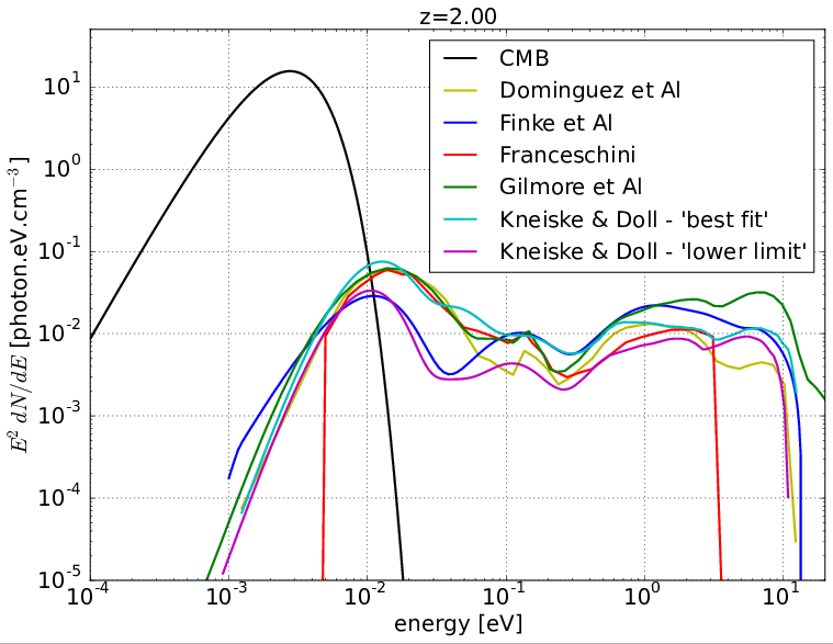
Figure 1: Comoving spectral energy distribution of target photons at a redshift $z=2$, including the Cosmological Microwave Background (black line) and different models of EBL (color lines).

The photon mean annihilation distance is plotted in Fig. 2 as a function of the initial photon energy, assuming the EBL model from Domínguez et al. (2011). The solid lines show the results for an expanding universe while the dashed lines show the results for a static universe. Below 1 TeV, the absorption mean free path quickly becomes larger than the typical distance of targeted sources (100 Mpc to Gpc), so that only TeV photons are significantly absorbed. Below 200-300 GeV, photons tend to travel over such large distances that two cosmological effects work in concert to produce a diverging mean free path. First, the target photon density vanishes as $(1+z)^{3}$ as the universe expands (horizon event). Second, gamma-rays photons are more and more redshifted before reaching the next annihilation point, requiring higher and higher energy target photons. As the EBL photon density drops at 10 eV, the mean free path diverges at low energy. Photons emitted at low redshift, with an energy of 1 TeV travel a few hundred Mpc before producing pairs. This distance decreases quickly at higher energy to reach few Mpc to few kpc. Considering a blazar like Mrk421 ($z=0.0308$, 135 Mpc) emitting very high-energy photons up to 100 TeV, primary gamma-rays are typically absorbed over a distance of a few Mpc.

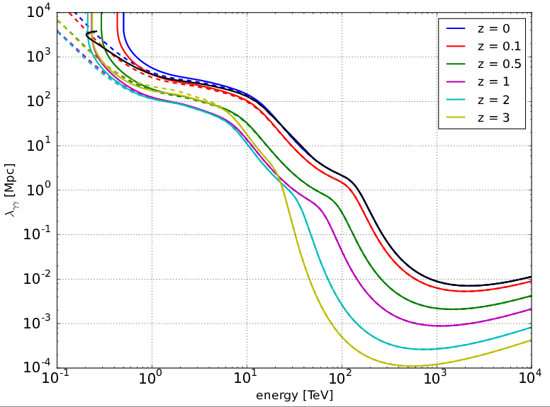
Figure 2: Gamma-ray annihilation mean free path $\lambda_{\gamma\gamma}=ct_{\gamma\gamma}$ (where $t_{\gamma\gamma}$ is the mean cosmic time between two interactions) as a function of their initial energy, and for different emission redshifts (solid lines). For comparison, the mean free path for a static universe (with properties frozen at their values at the initial redshift) is shown in dashed lines. The black line shows the thin/thick transition where the mean free path equals the source distance $D_{s}$ and where the energy equals the absorption energy $E_{\rm abs}$.

Since the density of the EBL photons decreases with their energy, gamma-ray absorption is more efficient at high energy. The transition from optically thin to optically thick photon-photon absorption where the radiation becomes fully absorbed occurs at an initial energy $E_{\rm abs}=(1+z)E_{\rm cut}$ where $E_{\rm cut}$ is the corresponding energy cut-off observed in the spectra at $z=0$. Fig. 3 shows the cut-off energy as a function of source redshift. Distant sources are more absorbed and their absorption occurs at lower energy. Significant differences are observed between the different EBL models. At large redshift ($z>1$), the different EBL models are very different, and differences up to a factor 6 are observed in the cutoff energy. At lower redshifts the EBL models are consistent with each other and only differ by a factor 2 at the lowest energies as, at such low distance, gamma-gamma absorption occurs mainly above 10 TeV. The effects of the EBL model on the cascades will be discussed in section 5.1.

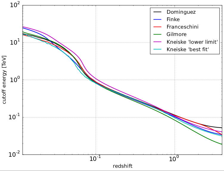
Figure 3: Cut-off energy $E_{\rm cut}$ observed at $z=0$ as a function of the source redshift for different EBL models.

2.3 Compton scattering by the CMB

High-energy leptons Compton up-scatter soft ambient photons to gamma-ray energies. In the Thomson regime, the Compton cross-section does not depend on the energy, and the scattering rate scales linearly with the target photon number density, hence Compton scattering mostly occurs on CMB photons. The CMB is modelled by a blackbody with a temperature $T_{\rm cmb}=(1+z)T_{\rm cmb,0}$ (Black curve in Fig. 1), where $T_{\rm cmb,0}=2.725$ K is the temperature at $z=0$. The associated CMB mean density, average energy and mean energy density are respectively:

$$n_{cmb} =16\pi\zeta(3)\left(\frac{k_{B}T_{\rm cmb}}{hc}\right)^{3}\approx 411(1+z)^{3}\quad\rm{cm}^{-3},$$ (2)

$$\epsilon_{cmb} =\frac{\pi^{4}}{30\zeta(3)}k_{B}T_{\rm cmb}\approx 6.34\times 10^{-4}(1+z)\quad\rm{eV},$$ (3)

$$\rho_{cmb} =n_{cmb}\epsilon_{cmb}\approx 0.26(1+z)^{4}\quad\rm{eV.cm}^{-3},$$ (4)

where $\zeta(3)\approx 1.202$, $k_{B}$, and $h$ are the Apéry’s, the Boltzmann’s, and the Planck’s constants respectively. In the Thomson regime, leptons of local energy $E_{e}$ up-scatter soft photons to typical energy:

$$E_{\gamma}=\frac{4\epsilon_{cmb}E_{e}^{2}}{3m_{e}^{2}c^{4}}\approx 3.23(1+z)\left(\frac{E_{e}}{1\rm{TeV}}\right)^{2}\quad\rm{GeV}.$$ (5)

Between two Compton scatterings, the leptons travel a Compton mean free path $\lambda_{ic}=1/(n_{cmb}\sigma_{T})\approx 1.19$ kpc (corresponding to a scattering time of $t_{ic}=\lambda_{ic}/c=3870$ yr), where $\sigma_{T}$ is the Thomson cross section. And on average, they loose energy at rate:

$$\frac{dE_{e}}{dt}=\frac{4}{3}c\sigma_{T}\rho_{cmb}\left(\frac{E_{e}}{m_{e}c^{2}}\right)^{2}.$$ (6)

After a flight of length $x$, the lepton energy is $E_{e}(x)=E_{e}^{0}/(1+x/D_{ic}^{0})$ where

$$D_{ic}^{0}=\frac{3m^{2}c^{4}}{4\sigma_{T}\rho_{cmb}E_{e}^{0}}\approx 367~{}(1+z)^{-4}\left(\frac{E_{e}^{0}}{1\rm{TeV}}\right)^{-1}\quad\rm{kpc},$$ (7)

is the initial Compton cooling distance, and $E_{e}^{0}$ is the lepton energy at the production site.

2.4 Observables

Based on these simple properties, some analytical estimates for typical cascade observables can be derived. Here we make the following standard assumptions:

• The source of primary gamma-rays is isotropic and mono-energetic with an energy $E_{\gamma}^{0}$.

• The primary gamma-rays all annihilate at exactly the same distance $\lambda_{\gamma\gamma}$ as given in Fig. 2.

• The leptons are produced by photon-photon annihilation in the direction of the parent gamma-ray photon and have exactly half of its energy.

• Compton interactions occur in the Thomson regime and the leptons travel exactly over one mean free path $\lambda_{ic}$ between two Compton scatterings.

• The leptons are deflected by a uniform magnetic field perpendicular to the motion.

• Magnetic deflections occur locally on scales much smaller than the photon annihilation length and the source distance.

• The scattered photons all get exactly the average energy given by equation 5 and are emitted in the propagation direction of the scattering lepton.

• The absorption of these scattered photons (hereafter refereed to as first generation photons) and the associated pair production is neglected. The contribution of higher generation particles is not considered.

• Cosmological effects are neglected.

With the above assumptions we can derive the following cascade geometrical and distribution properties:

Geometry:

Geometrical effects (halo effects and time delay) are due to the lepton deflection in the extragalactic magnetic field. Two cases can be studied:

• If the coherence length is large ($\lambda_{B}\gg D_{ic}^{0}$) the magnetic field can be considered as uniform and the lepton deflection after a travel distance $x$ is: $\delta=\int_{0}^{x}ds/R_{L}(s)$. It means that a lepton of initial energy $E_{e}^{0}=E_{\gamma}^{0}/2$ having cooled down to energy $E_{e}$ has been deflected from its original trajectory by an angle:

  $$\delta=\frac{D_{ic}^{0}}{2R_{L}^{0}}\left[\left(\frac{E_{e}^{0}}{E_{e}}\right)^{2}-1\right],$$ (8)

  where $R_{L}^{0}$ (Eq. 1) is the initial Larmor radius of the lepton. As soon as the lepton has lost a significant fraction of its energy, the previous equation reduces to:

  $$\delta\approx\frac{D_{ic}}{2R_{L}}=\frac{e_{c}B\lambda_{ic}}{2E_{\gamma}},$$ (9)

  where $D_{ic}$ and $R_{L}$ are no longer the initial values but are now evaluated locally at energy $E_{e}\ll E_{e}^{0}$, corresponding to photons scattered to energy $E_{\gamma}$ (Eq. 5).

• If the coherence length is short ($\lambda_{B}\ll D_{ic}^{0}$), the leptons travel across many zones of a highly turbulent field. We assume that the field is composed of many cells of size $\lambda_{B}$, with uniform field and random directions. In each cell, the leptons are deflected by an angle $\sim\lambda_{B}/R_{L}$ in a random direction. Considering this process as a random walk leads to:

  $$\delta =\frac{\sqrt{D_{ic}^{0}\lambda_{B}}}{2R_{L}^{0}}\left[\left(\frac{E_{e}^{0}}{E_{e}}\right)^{2}-1\right]$$

  $$\approx\frac{\sqrt{D_{ic}\lambda_{B}}}{2R_{L}},$$ (10)

  where the last approximation is obtained similarly to Eq. 9.

In both cases, the magnetic deflection is a function of the lepton energy $\delta(E_{e})$ and of the secondary gamma-ray energy $\delta(E_{\gamma})$. In the following, we will concentrate on large-coherence case ($\lambda_{B}\gg D_{ic}^{0}$). However, similar constraints are easily obtained for short coherence lengths.

The geometrical properties of the cascade (extension, time delay) can be derived from the magnetic deflection angle (e.g. Neronov & Semikoz, 2007; Dermer et al., 2011). They are illustrated in Fig. 4.

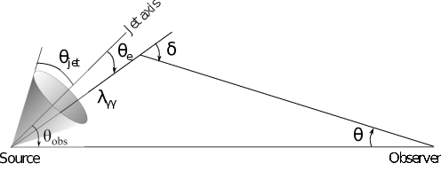
Figure 4: Geometry of the one-generation model.

In the one-generation approximation, halo photons observed with a finite angle $\theta$ were emitted out of the line of sight and then deflected back to the observer. Assuming the lepton deflection occurs on very short distances compared to the photon absorption length, the detection angle and time delay are:

$$\theta =\arcsin\left(\frac{\lambda_{\gamma\gamma}}{D_{s}}\sin\delta\right)\approx\frac{\lambda_{\gamma\gamma}}{D_{s}}\delta,$$ (11)

$$c\Delta t =\lambda_{\gamma\gamma}(1-\cos\delta)-D_{s}(1-\cos\theta)\approx\lambda_{\gamma\gamma}\frac{\delta^{2}}{2},$$ (12)

where $D_{s}$ is the distance to the source, $\lambda_{\gamma\gamma}$ is the annihilation distance of the primary photons, and where the last approximations were obtained in the small-angle approximation ($\lambda_{\gamma\gamma}\ll D_{s},\delta\ll 1$). These relations are illustrated in Figs. 5 in the case of large coherence length.

As high-energy leptons travel and get deflected, the detection angle and time delay decrease as energy increases. In this regime, the small angle approximation is well satisfied and for large coherence length ($\lambda_{B}\gg D_{ic}^{0}$) the latter equations combined to Eq. 5 and 9 yield respectively to:

$$\theta \approx 0.79^{\circ}\left(\frac{\tau_{\gamma\gamma}}{397.4}\right)^{-1}\left(\frac{B}{10^{-14}\,\textrm{G}}\right)\left(\frac{E_{\gamma}}{1\,\textrm{GeV}}\right)^{-1},$$ (13)

$$\Delta t \approx 65\left(\frac{\lambda_{\gamma\gamma}}{1.32\rm Mpc}\right)\left(\frac{B}{10^{-17}\textrm{G}}\right)^{2}\left(\frac{E_{\gamma}}{1\,\textrm{GeV}}\right)^{-2}\,\textrm{yrs},$$ (14)

where $\tau_{\gamma\gamma}=D_{s}/\lambda_{\gamma\gamma}$ is the annihilation optical depth. All values are calculated for a source at $z=0.13$ emitting primary photons at $E_{\gamma}^{0}=100$ TeV. These equations show the complementarity in the search for pair halos and pair echoes. Pair halos can only be observed if they are larger than the instrument point spread function (PSF). For a typical PSF of $0.1^{\circ}$, the above values correspond to magnetic fields larger than $10^{-14}$ G. Hence, large magnetic field strengths can be constrained through detection of pair halos. In this case, time delays are as long as $10^{8}$ yrs and echoes cannot be observed. On the other hand, still with the values above, observable echoes shorter than $5$ yr require magnetic fields lower than $10^{-18}$-$10^{-17}$ G. Hence low magnetic field strengths can be constrained though detection of pair echoes. In that case, pair halos are typically smaller than $0.0001^{\circ}$ and cannot be resolved.

As the lepton energy decreases, both the detection angle and the time delay increase until the maximal deflection $\delta=\pi/2$ is reached for which $\theta_{\rm max}\approx 1/\tau_{\gamma\gamma}=5.7^{\circ}(\tau_{\gamma\gamma}/10)^{-1}$. This corresponds to the maximal halo size. At a lower lepton energy, the Larmor radius becomes smaller than the magnetic coherence length. The leptons are trapped by the magnetic field and cannot travel farther. This leads to the formation of a cloud of $e^{+}-e^{-}$ pairs around the source. The size of the observed halo then corresponds to the physical extension of the pair cloud, i.e. $\lambda_{\gamma\gamma}$.

Distributions:

In the following, unless otherwise specified, all distributions are normalised to one single primary photons emitted.

The cascade spectrum produced by one single high-energy photon is computed as $dN/dE_{\gamma}=2(dN/dt)_{ic}/(dE_{\gamma}/dE_{e})/(dE_{e}/dt)$, where the factor 2 accounts for the two leptons produced by one single primary photon. Noting that the number of photons up-scattered by one lepton per unit time is $(dN/dt)_{ic}=c/\lambda_{ic}$, and using Eq. 5 and 6 to derive the last terms leads to:

$$E_{\gamma}^{2}\frac{dN}{dE_{\gamma}}=\frac{m_{e}c^{2}}{2}\sqrt{\frac{3E_{\gamma}}{\epsilon_{cmb}}}\approx 556\left(\frac{E_{\gamma}}{1\,{\rm GeV}}\right)^{1/2}(1+z)^{-1}\textrm{GeV}.$$ (15)

It is a simple power-law $dN/dE_{\gamma}\propto E_{\gamma}^{-\Gamma}$ with index $\Gamma=3/2$. If unabsorbed, this spectrum extends up to the energy of photons scattered by the highest-energy leptons, i.e. $E_{\gamma,\rm max}=0.8\left(E_{\gamma,0}/1~{}{\rm TeV}\right)^{2}$ GeV. However, for distant sources, such a power-law spectrum is typically cut at lower energies by photon absorption (Fig. 3). In principle, a new generation of particles is then produced. Higher photons generation have often been neglected although they may contribute significantly to the overall spectrum (see section 3).

The angular distribution can be computed as $dN/d\theta=(dN/dE_{\gamma})(dE_{\gamma}/d\delta)(d\delta/d\theta)$. Using Eq. 15, 9, and 11 to estimate the three factors respectively allows to derive the angular distribution of first-generation photons produced by one single primary photon, for large coherence length and small angle:

$$\theta\frac{dN}{d\theta} =m_{e}c^{2}\left(\frac{3}{2\lambda_{ic}\epsilon_{\rm cmb}}\frac{\tau_{\gamma\gamma}\theta}{e_{c}B}\right)^{1/2}$$

$$=1972.3\left(\frac{\tau_{\gamma\gamma}}{397.4}\right)^{1/2}\left(\frac{B}{10^{-15}\rm G}\right)^{-1/2}\left(\frac{\theta}{1^{\circ}}\right)^{1/2}.$$ (16)

Identically, writing $dN/dt=(dN/dE_{\gamma})(dE_{\gamma}/d\delta)(d\delta/dt)$ and using Eq. 12 gives the following distribution of time delays:

$$\Delta t\frac{dN}{dt} =m_{e}c^{2}\left(\frac{3}{4\lambda_{ic}\epsilon_{cmb}e_{c}B}\right)^{1/2}\left(\frac{c\Delta t}{2\lambda_{\gamma\gamma}}\right)^{1/4}$$

$$=437.2\left(\frac{\lambda_{\gamma\gamma}}{1.32\rm Mpc}\right)^{-1/4}\left(\frac{\Delta t}{10^{6}\rm yr}\right)^{1/4}\left(\frac{B}{10^{-15}\rm G}\right)^{-1/2}.$$ (17)

These distributions are pure power-laws and do not show any specific angular (or time) scale because they are composed by the contributions of photons detected with all possible energies. However, as discussed below, real observations are obtained in a limited energy range, with a given aperture angle, and with a finite observation duration. This produces characteristic scales in energy, arrival angle and time delay, that appear as cuts or breaks in the corresponding distributions.

3 Code description and test cases

The analytical approximations presented in the previous sections are useful to understand the physics of the cascades and to obtain orders of magnitude estimates, but accurate calculations require numerical simulations. For this purpose, we have developed a new Monte Carlo code. In this section, we outline the main features of this code and compare its results to the analytical predictions presented in section 2.4 as well as to other published results.

3.1 Code and simulation set-up

Our Monte Carlo code is designed to track the propagation of all particles and to reproduce the properties of the cascade as precisely as possible. A complete description of the code can be found in appendix A. However, the main algorithm is summarised here (see also Fig. 21):

• Primary particles (photons or leptons) are launched at a given redshift and with a given energy. Particle energy can also be sampled from a power-law distribution. In this paper will focus only on cascades initiated by photons.

• Interaction distances are generated randomly according to the probability distribution given by the exact cross-sections ($e^{+}-e^{-}$ pair production for a photon, Klein-Nishima cross-section for a lepton) and taking into account the cosmological evolution of the target particles.

• The particles are propagated taking into account all cosmological effects (redshift, expansion). In particular, the transport of leptons in the EGMF is computed as described in appendix A.1. If the particles interact before reaching the Earth, the interaction outcome is computed. Energy and direction of the outcoming particles are generated according to the probability distributions given by the exact differential cross-sections. Particles with updated parameters and new particles are then stored for later treatment. The physical parameters of the particles reaching the Earth without any interaction are stored for post-processing.

• The extragalactic magnetic field is modeled by dividing the comoving space into a number of cells with size $\lambda_{B}$, defining regions of uniform magnetic field. For each cube a random magnetic field direction is computed and is kept for the entire simulation. The EGMF is set by its strength at redshift $z=0$. For very short coherence lengths, the lepton interaction distance ($\lambda_{IC}\approx 1$ kpc) can become larger than $\lambda_{B}$. In such a case, the motion to the next interaction location is divided in shorter steps of length a fraction of $\lambda_{B}$, to ensure that the leptons are deflected by all cells.

The following subsections present the results of test simulations. For the sake of comparison, we first consider a simple canonical model consisting in a mono-energetic source (100 TeV) emitting isotropically at z=0.13 (around 557 Mpc). We use the EBL model of Domínguez et al. (2011). With this set-up the characteristic annihilation distance of primary photons is $\lambda_{\gamma\gamma}=1.32$ Mpc. The EGMF is set to $B=3\times 10^{-16}$ G with a coherence length of $\lambda_{B}=1$ Mpc.

We focus on the three main observables characterising the photons detected on Earth: their energy, their arrival angle, and their time delay. We derive the 3D photon distribution in this space of parameter. We also concentrate on the contribution of the different generations of particles, i.e. their rank in the cascade tree. In the following, the zeroth generation corresponds to the primary photons emitted at the source. These photons annihilate, produce pairs, that in turn produce the photons of first generation. Again, these can produce pairs which up-scatter target photons producing the second photon generation, and so on. As we are only interested in the detection of photons, their energy will be written $E$, where the subscript $\gamma$ has been dropped for simplicity.

3.2 Correlations between observables

In the framework of the approximations used in the one-generation analytical model, the photon energy, detection angle and time delay are linked exactly through simple relations. When these approximations are relaxed a significant scatter is expected. Fig. 5 show the three possible correlations between the photon energy $E$, the detection angle $\theta$, and the time delay $\Delta t$.

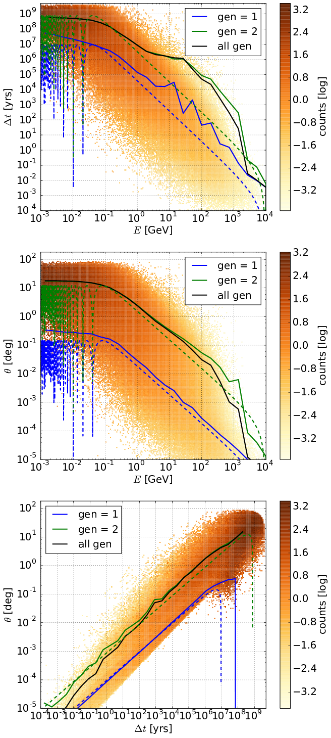
Figure 5: Top panel: Correlation between the time delay $\Delta t$ and energy $E$ of detected photons. The density map shows the number of photons per unit energy and time delay $(E\Delta t)d^{2}N/(dEd\Delta t)$ with a log color scale. The blue, green and black solid lines show the average time delay for first-generation photons only, second-generation photons, and all photons, respectively. The blue and green dashed lines show the analytical estimates for the first and second generations only (see sec. 2.4). With the same notations, the middle and bottom panels show the energy-detection angle and detection angle-time delay correlations respectively.

In addition, the average behaviour is plotted in solid line for each generation by binning the x-axis (with 4 bins per decade) and averaging the y-values. The analytical estimates of the one-generation model (from Eq. 11 and 12) are shown for comparison as blue, dashed lines. The expected trends are recovered: the smaller the energy, the larger the observation angle and the arrival time delay. As the leptons cool down, they produce more and more gamma-ray photons per unit time. As a result, the total cascade emission is dominated by a very large number of photons with low-energy, large angle, long time delay, as can be seen in Fig. 5. However, several important points can be made.

The averaged values for the first-generation photons (blue line) are consistent with the analytical results of sec. 2.4: both the saturation at low energy and the slopes in the small-angle regime are well recovered. The saturations observed in time correspond to the maximal delay (photons that are emitted away from, and scattered back to the observer) while the saturation observed in detection angle corresponds to photons deflected by an angle of $\delta=\pi/2$. The power-law regimes correspond to Eq. 13 and 14. Most of the observed deviations at high energy (e.g. fluctuations and peaks) come from the limited statistics of the simulations: averaged values can be contaminated by a few photons with very large values (typically photons scattered by EBL targets instead of CMB photons). Physical processes that are not taken into account in the analytical estimates (Klein-Nishina regime, dispersion in the annihilation distance, non-uniform magnetic field, energy dispersion around the averaged value …) are also responsible for deviations to the approximations, but the effects are weaker.

These results also show that the one-generation model underestimates the detection angle and the time delay by at least two orders of magnitude when the contribution of second-generation photons is significant. Indeed the highest energy, second-generation photons are almost all produced at the location where the parent leptons which emitted them where produced. As these photons have lower energy than the primary photons, their annihilation distance is larger $\lambda_{\gamma\gamma}^{gen=1}\gg\lambda_{\gamma\gamma}^{gen=0}$. As a result, the highest energy, second-generation photons are typically produced at a distance $\lambda_{\gamma\gamma}^{gen=1}$ from the source. The geometry remains however similar so that an estimate for the second-generation observable quantities can be found by substituting $\lambda_{\gamma\gamma}$ by $\lambda_{\gamma\gamma}^{gen=1}$ in the results of sec. 2.4. For primary photons at 100 TeV, the highest-energy, first-generation photons ($8$ TeV) have mean free path $\lambda_{\gamma\gamma}^{gen=1}=117$ Mpc. This is shown in Fig. 5 as green dashed lines. As can be seen, this new estimate matches well the average results of second-generation dominated cascades.

We emphasise that a single generation never dominates at all energies, angles and time delays. In our canonical simulation for instance, only the low-energy spectrum is dominated by second-generation photons while the highest energy photons are mostly first-generation photons (see Fig. 6). This is why the average time delay drops below the second-generation estimates at high energy.

In principle, the ratio of first to second generation photons depends on the energy of primary photons and the source distance. If primary photons have energy smaller than or close to the absorption energy $E_{\rm abs}$, then the absorption is so weak that the production of second-generation photons is quenched, and the cascade is dominated by first-generation photons (this will be illustrated in Fig. 12 for instance). However, the results presented here remain general as soon as the energy of primary photons is significantly larger than the absorption energy (see also Berezinsky & Kalashev, 2016).

In any case, there is a large dispersion around the average quantities, showing that the latter might be of limited practical use.

3.3 Photon distributions

The energy, angle and time distributions are obtained by integrating over the other two parameters. In this section we focus on photons with energy above 1 GeV which corresponds to the typical energy range of gamma-ray observatories.

The spectrum of our fiducial model, integrated over the entire sky, over all possible arrival times, and normalised to one primary photon, is shown in Fig. 6. It is compared to Fig. 1 of Taylor et al. (2011) and to the results of the Elmag code (Kachelriess et al., 2012) using the same set-up. Spectral shapes provided by the different codes are compatible each other.

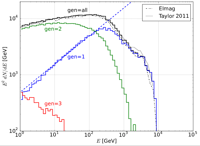
Figure 6: Full spectrum for an isotropic and mono-energetic source (100 TeV) at $z$=0.13 (black line). The blue, green and red lines show the contributions of generations 1, 2 and 3 respectively. The analytic expression (Eq. 15) is shown in blue dashed line. The dotted-dashed, and dotted lines show the results from Elmag (Kachelriess et al., 2012) and Taylor et al. (2011) respectively.

All primary photons at 100 TeV are absorbed and produce the first-generation spectrum (blue line). Below $E_{\rm cut}$ analytical estimates (Eq. 15) are well reproduced by the first-generation population, in spite of the approximations made. Above 1 TeV the photon of the first generation are absorbed (Fig. 3) and produce a second generation which dominates the spectrum below about 100 GeV (green line). The spectrum of the second generation is similar to the spectrum of the first generation ($dN/dE\propto E^{-3/2}$) except it is softer in the energy range shown in this figure (it can be shown that $dN/dE\propto E^{-7/4}$). A few second-generation photons are also absorbed and produce a weak third-generation population (red line) which does not contribute to the total spectrum.

The angle distribution integrated over energies $E>1$ GeV and over all arrival times, normalised to one primary photon is shown in Fig. 7.

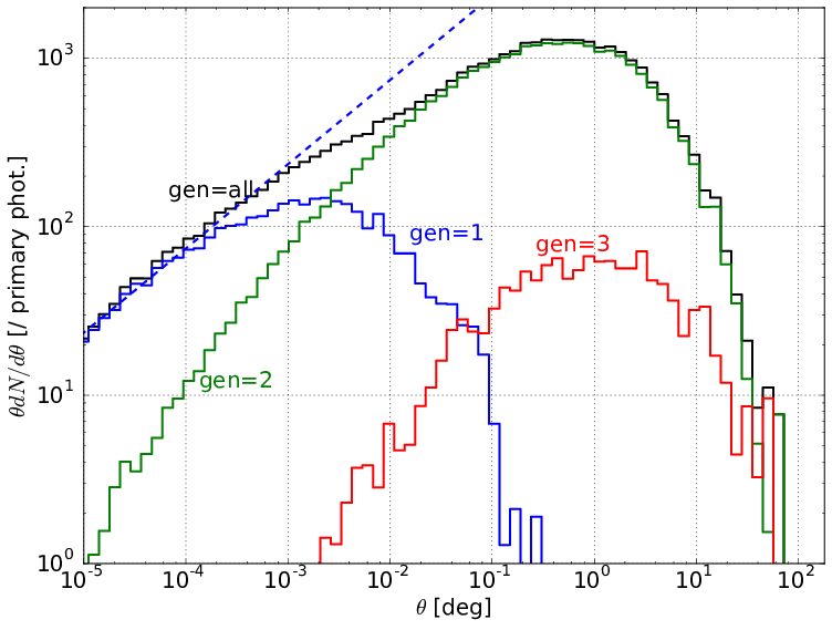
Figure 7: Detection angle distribution for $E>1$ GeV photons. The colors are the same as in Fig. 6. The blue, dashed line shows the analytical estimate of Eq. 16.

The emission is peaked at the center and decreases as a power-law with increasing angle. At small angles, the distribution of first-generation photons is well approximated by the analytical estimate given in Eq. 16: $dN/d\theta\propto\theta^{-1/2}$. However, only photons above 1 GeV are considered here. Hence, low-energy photons with large angles are not observed. And, as compared to the analytical estimate, the angular distribution drops at a typical size that depends on the minimal energy and the magnetic field. As second-generation photons have a larger mean free-path, they typically arrive with larger angles. Interestingly, the distribution is dominated by second-generation photons at observable scales ($\theta>0.1^{\circ}$). This result remains general as long as the energy of primary photons is significantly larger than the absorption energy $E_{\rm abs}$ (i.e. photons have absorption depth $\tau_{\gamma\gamma}(E^{0})>>1$). Primary photons with energy comparable to the absorption energy ($\tau_{\gamma\gamma}(E^{0})\approx 1$) are weakly absorbed and do not produce high-generation photons. For sources with an extended intrinsic spectrum, the contribution of first- and second-generation photons to the angular distribution is more complex (see sec. 4.2).

The time delay distribution integrated over energies $E>1$ GeV and all detection angles, and normalised to one primary photon, is shown in Fig. 8.

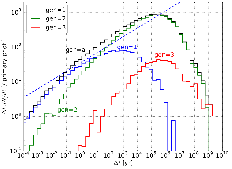
Figure 8: Distribution of time delays for $E>1$ GeV photons. The colors are the same as in Fig. 6. The blue, dashed line shows the analytical estimate of Eq. 17.

As time evolves after a source flare, less and less photons are observed. The one-generation model (Eq. 17) provides a good estimate of the first-generation distribution for time delays ranging from about 1 month to 100 years. Shorter time delays correspond to high energy photons that are absorbed, producing a drop below the analytical estimate. Longer time delays correspond to low-energy photons below the selection criterion $E>1$ GeV, producing a cut of the distribution above 1000 years. Interestingly, accessible time delays ($\Delta t<1$ yr) after a flaring event (such as a GRB) are short enough to be dominated by first-generation photons only, allowing for the use of simple formulae to derive constraints from the potential detection of pair echoes.

The three distributions presented on Figs. 6, 7 and 8 ($dN/dE$, $dN/d\theta$, and $dN/dt$) are global distributions in the sense that they are integrated over large ranges of the 2 others quantities. For instance, the spectrum shown in Fig. 6 is the integrated over all detection angles and all arrival times. However, in a more realistic situation, only limited ranges of these quantities are accessible. As low-energy photons arrive with large angle, large time delay, and are products of primary photons emitted far away from the line of sight, any of the following effects will damp the spectrum at low energy, while cutting the large angle and large time delay part of the associated distributions:

1. If the instrument is only sensitive above a given energy (see discussion before).

2. If the instrument aperture is limited.

3. If the exposure time is finite after an impulsive flaring event.

4. If the source emission is beamed within a limited opening angle.

The effect of finite exposure time is illustrated in Fig. 9 (see also Ichiki et al., 2008).

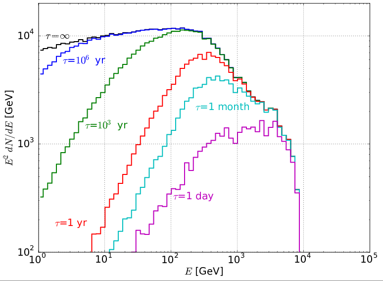
Figure 9: Total spectrum of an flaring event integrated over a finite exposure time ($t_{\rm obs}=\tau$), or equivalently: instantaneous spectrum of a source that has been active for a give time ($t_{\rm act}=\tau$) in the past.

This can be interpreted in two ways. If the source produces a strong, impulsive flaring event (such as a GRB for instance), this figure shows the integrated spectra as data is accumulated from the detection of the unabsorbed, primary photons up to time $t_{\rm obs}=\tau$. As time evolves lower energy photons are detected and the low-energy part of the spectrum builds up slowly. Alternatively, this figure also shows the instantaneous spectra observed at present time, if the source (such as an AGN) has been active for a time $t_{act}=\tau$ in the past, with constant luminosity (Dermer et al., 2011). As the activity period increases, we are able to detect secondaries produced by primaries emitted earlier. As leptons had more time to cool down, these secondaries have lower energy. As a result, long activity sources have spectra that extend to lower energy.

4 Source properties

The simple case presented in section 3 allows us to understand general behavior of electromagnetic cascades. However, several effects must be included to produce realistic cascades. Gamma-ray sources (AGNs, GRBs) do not emit photons at a single energy or isotropically but instead produce non-thermal, beamed radiation. Here we investigate the following intrinsic properties of the source:

• Redshift $z$.

• Intrinsic spectrum: here we consider power-law spectra in the form $dN/dE\propto E^{-\Gamma}$ for $100$ MeV$\geq E\geq E_{\rm max}$.

• Emission profile: here we assume a disk emission, i.e. an axisymmetric angular distribution $dN_{e}/d\Omega_{e}$ uniform up to a given half-opening angle $\theta_{\rm jet}$ observed with an angle $\theta_{\rm obs}$ away from its axis (see Fig. 4).

In the following we use simulation parameters corresponding to the Blazar 1ES0229+200 (Tavecchio et al., 2009; Taylor et al., 2011; Vovk et al., 2012) with a redshift $z=0.14$ corresponding to a distance of 599 Mpc, and a hard spectrum with $\Gamma=1.2$. The unconstrained maximal energy of the intrinsic spectrum is set to $E_{\rm max}=100$ TeV and the emission is assumed to be isotropic. The EGMF has an averaged intensity of $B=10^{-15}$ G, and a coherence length $\lambda_{B}=1$ Mpc. We use the EBL model of Domínguez et al. (2011).

In this section, the spectra are normalised to $L_{0}$, the intrinsic luminosity of the source as observed at $z=0$ (i.e. the intrinsic luminosity decreased by a factor $1+z$).

4.1 Source redshift

The spectral evolution with redshift is shown in Fig. 10 for $z=0.04$ ($D_{s}\sim 175$ Mpc), $z=0.14$ ($D_{s}\sim 599$ Mpc), $z=1$ ($D_{s}\sim 3.4$ Gpc), and $z=2$ ($D_{s}\sim 5.3$ Gpc).

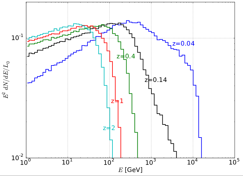
Figure 10: Full spectrum of sources at different redshifts ($z=0.04$, $0.14$, $0.4$, $1$ and $2$), normalised to the intrinsic luminosity attenuated by a factor $1+z$ to account for the universe expansion.

As expected, the cut-off energy decreases with increasing distance as the column density of target photons increases. At high redshift, we find that the absorption depth goes simply as $\tau_{\gamma\gamma}\propto E^{2}$ producing a super-exponential cutoff $\propto e^{-E^{2}/E_{\rm cut}^{2}}$. However the spectra of nearby sources show a more complex and harder absorption cutoff. In our setup, the maximal energy of primary photons (100 TeV) is large enough to generate an efficient cascade. As a result, almost all shown spectra are dominated by second-generation photons. Only when the source is close enough ($z=0.04$), the absorption is weak enough to quench the production of second-generation photons. As discussed by Berezinskii & Smirnov (1975) the spectrum softens as the generation order increases, which is consistent with the harder spectrum observed at $z=0.04$. The intrinsic spectrum used here is hard ($\Gamma=1.2$), so that most of the intrinsic luminosity is concentrated at the highest energies ($E_{0}\sim E_{\rm max}$). Most of the spectrum is then fully absorbed and redistributed as cascade contribution. As a result, the amplitude of the observed spectra is almost insensitive to the absorption energy, i.e. also to the source redshift.

The evolution of the angular distribution and time delays of photons with energy $E>1$ GeV, are illustrated by their average values in Fig. 11 for different EGMF strengths.

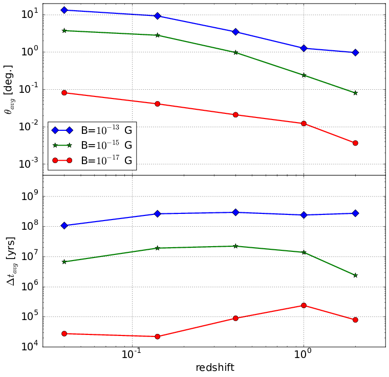
Figure 11: Average arrival angle (top) and time delay (bottom) of photons with energy $E>1$ GeV, as a function of the source redshift, for different EGMF strengths ($B=10^{-13},10^{-15}$, and $10^{-17}$ G).

Both the halo extension and the time delay increase with magnetic field, as leptons of given energy are more deflected by stronger fields. Their evolution with redshift is the result of several effects. The halo extension decreases with distance. To zeroth order, it is simply due to geometrical effects: the same annihilation distance to the source corresponds to a smaller angle as seen from a more distant observer (see for instance Eq. 11 for first-generation photons: $\theta\propto\lambda_{\gamma\gamma}/D_{s}$). In contrast, the time delay does not suffer from any geometrical dependence on distance (see for instance Eq. 12 for first-generation photons) and shows only little evolution with redshift. To first order however, the cosmological evolution of the universe also influences the angular size and time delay of secondary photons (namely through $\lambda_{\gamma\gamma}(z)$, $\lambda_{ic}(z)$, $B(z)$, and $E(z)$), explaining the remaining evolution.

4.2 Source spectrum

Fig. 12 shows the observed spectra when the source intrinsic spectrum is changed.

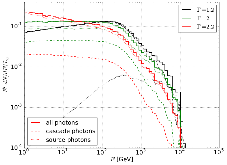
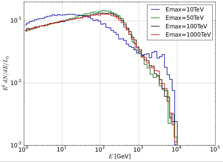
Figure 12: Top panel: Observed spectra for $E_{\rm max}=100$ TeV and different spectral indices $\Gamma$ (solid lines) . The contributions of the primary source and the cascade are shown in dotted and dashed lines respectively. Spectra are normalised to $L_{0}$, the intrinsic luminosity attenuated by $1+z$. Bottom panel: Spectra for $\Gamma=1.2$ and different maximal energies $E_{\rm max}$.

The top and bottom panel show the results for different spectral indices ($\Gamma$=1.2, 2 and 2.2, $E_{\rm max}=100$ TeV) and different maximal energies ($E_{\rm max}=10$, 50, 100 TeV and 1 PeV, $\Gamma=1.2$) respectively. At source distance $z=0.14$, photons with energy higher than a few TeV are absorbed and redistributed towards low energies. For hard spectra ($\Gamma<2$), many primary photons are absorbed. This induces a strong cascade which dominates the intrinsic source emission at all energies. The observed spectrum is very similar to the mono-energetic model shown in Fig. 6. In contrast, when the intrinsic spectra are soft ($\Gamma>2$), only few primary photons are absorbed. The cascade contribution is negligible and only the absorbed, intrinsic spectrum is observed. As far as only the cascade emission is concerned (dashed lines), the spectrum is only weakly dependent on the intrinsic hardness. This strong universality of the cascade emission is also illustrated in the bottom panel where the shape of the observed spectrum is highly insensitive to the maximal energy, Only the case with $E_{\rm max}=10$ TeV shows significant departure from the generic spectral shape. In that specific case, the intrinsic spectrum does not extend much beyond the absorption energy $E_{\rm abs}$ at that distance, and the spectrum is dominated by first-generation photons which were produced below the average annihilation distance.

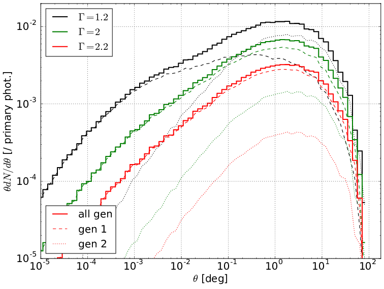
Figure 13: Angular distribution of $E>1$ GeV photons, for different intrinsic spectral indices $\Gamma$ and $E_{\rm max}=100$ TeV (solid lines). The dashed and dotted lines show the contributions of first-generation photons and second-generation photons respectively.

Fig. 13 shows the angular distribution in the 1 GeV-1 TeV band, for different intrinsic spectral indices. As can be seen, the angular distribution is rather insensitive to the intrinsic spectrum. Although the angular distribution of cascades induced by one single primary photon depends on the energy of this primary (it scales as $\lambda_{\gamma\gamma}(E_{0})$, see Eq. 13), two effects contribute to keep the final distribution induced by an extended intrinsic spectrum quite universal. First, most of the cascade is induced by primary photons just above the absorption threshold (see Fig. 3), i.e. in the 1-10 TeV range, because they are more numerous. In this range the mean absorption length is rather insensitive to the primary energy (see Fig. 2). Second, when the intrinsic spectrum extends to higher energy and is hard enough ($\Gamma\lesssim 2$), part of the cascade is in principle also induced by these high-energy photons with shorter absorption length. However the first-generation photons produced by these high-energy primaries are also absorbed. They produce second-generation photons that eventually dominate the angular distribution and have larger absorption depth (see sec. 3.2). Here also, the second-generation photons contribute dominantly to the cascade when they have energy just above the absorption energy, that is when they have absorption length comparable to that of low-energy primaries. This makes the spectrum insensitive to the energy of primary photons, that is to the intrinsic spectrum. The time delay distribution is even less sensitive to the properties of the intrinsic spectrum, and is not shown here.

These results show that the emission properties of cascades (spectrum, angular distribution and time distribution) do not depend on the properties of the intrinsic spectrum as long as the maximal energy of the source is large enough compared to the absorption energy. Although the cascade properties are highly dependent on several other parameters such as the distance and the EGMF, this illustrates the universal properties of the cascade emission with respect to the source intrinsic spectrum (e.g. Berezinsky & Kalashev, 2016).

4.3 Source beaming

Anisotropic emission can be modelled at the post-processing stage if the source emission is axisymmetric (e.g. a beamed emission) and the intergalactic medium is isotropic (see appendix A.4). If the source axis is not aligned with the line of sight, a jet structure is observed in the cascade emission (Neronov et al., 2010; Arlen et al., 2014). This is illustrated in Fig. 14.

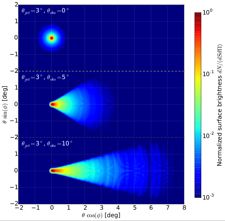
Figure 14: Images of a misaligned source at $z=0.14$, emitting a power-law spectrum with index $\Gamma=1.2$ in a uniform cone of half-opening angle $\theta_{\rm jet}=3^{\circ}$. Here $B=10^{-15}$ G, and $\lambda_{B}=1$ Mpc. Observations at three angles at shown: $\theta_{\rm obs}=0^{\circ}$, $5^{\circ}$, $10^{\circ}$ from top to bottom.

The general analysis of the misaligned case is beyond the scope of the current paper. In the following, we shall concentrate on the case of a beamed emission aligned with the line of sight.

The effect of the jet half-opening angle $\theta_{\rm jet}$ on the observed spectrum is shown in Fig. 15.

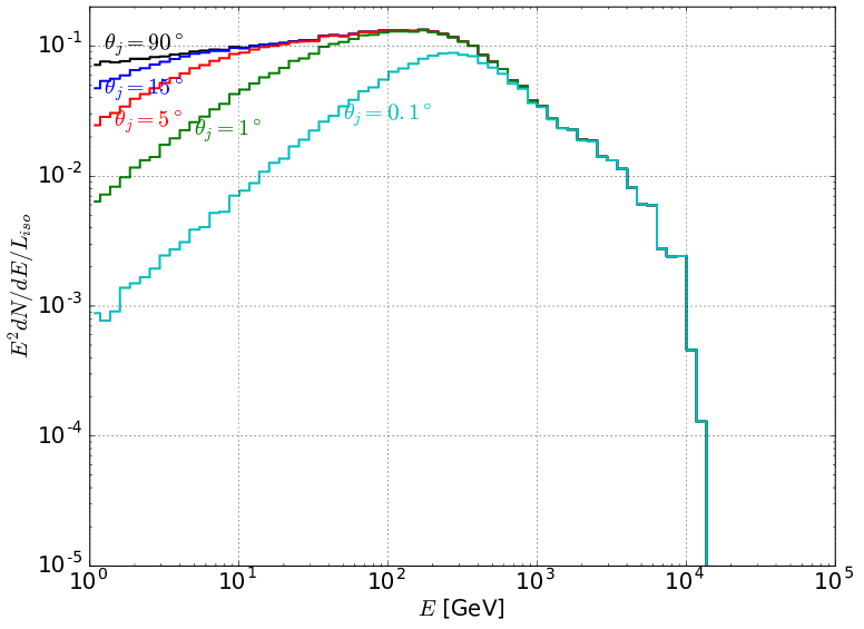
Figure 15: Energy spectra for different jet half-opening angles $\theta_{\rm jet}$. All spectra are normalised to the luminosity of an isotropic source of equal flux inside the emission cone: $L_{\rm iso}=2L_{0}/(1-\cos\theta_{\rm jet})$.

Lower energy photons typically originate from primary photons emitted farther away from the line of sight. Therefore in the case of a beamed source with no photon emitted at large angle, the cascade emission is suppressed below some critical energy (see for instance Tavecchio et al., 2010). Then, the more collimated the jet, the larger the critical energy. The precise transition energy depends on the magnetic field strength and coherence length. Although its value can be derived in the framework of a one-generation model, such results do not apply to sources emitting at high energy and producing high-generation dominated cascades.

The effect of the jet opening angle on the observed angular distribution and time delays is illustrated in Fig. 16 for different source distances.

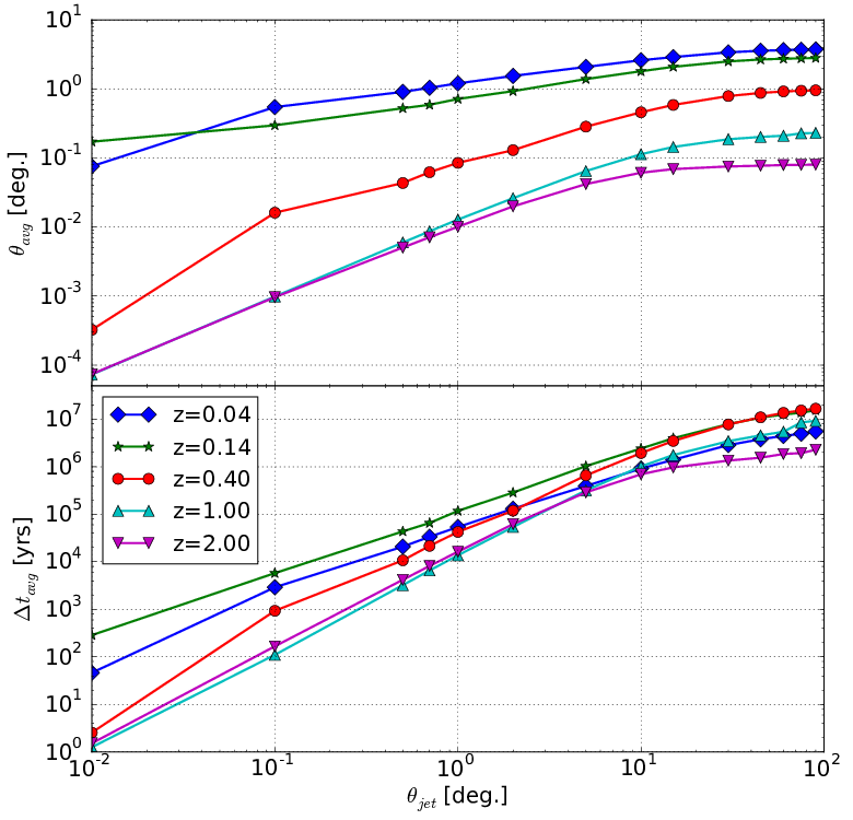
Figure 16: Average detection angle (top) and time delay (bottom) of photons with energy $E>1$ GeV as a function of the jet opening angle for sources at different redshifts.

Photons emitted with a large angle $\theta_{e}$ with respect to the line of sight are typically observed with a large angle $\theta\approx\theta_{e}/\tau_{\gamma\gamma}$. As a result, the averaged detection angle in the 1 GeV - 100 TeV band is expected to scale as $\langle\theta\rangle\ \propto\ \theta_{\rm jet}$. This is clearly observed for distant sources with $z>0.4$ at small angle. The increase of the average angle with the jet opening angle is less pronounced for nearby sources. This results from a combination of the source intrinsic spectrum (different primary energies correspond to different annihilation distances) and the complex absorption feature for nearby sources (see Fig. 10 and the associated discussion). At larger jet opening angle, the average detection angle is limited by the physical extension of the halo around the sources. For all opening angles, the average angle decreases with the source redshift mostly because of geometrical effect (halos look smaller when observed from larger distances).

The average time delay increases with the jet opening angle. Indeed with a large jet opening, there is a larger halo effect. Then photons are more deflected and arrive at latter times. The redshift dependence is less pronounced than that of the average angle, as already mentioned.

These results show that the effect of the source beaming on the cascade properties cannot be modelled by simple one-generation models, and that it must be investigated numerically.

5 Properties of the intergalactic medium

In section 4 we explored the effect of the source parameters on the development and observability of a cosmological cascade. We now illustrate the impact of the intergalactic medium, in particular the effects of:

• the extragalactic background light model

• the extragalactic magnetic field (amplitude $B$ and coherence length $\lambda_{B}$)

The same fiducial simulation is used, as in section 4.

5.1 Extragalactic background light

The extragalactic light (EBL) affects the absorption of gamma-rays. Fig. 17 shows the spectrum computed for an isotropic source with a spectral index of $\Gamma=1.2$ at a redshift $z=2$ using 6 different EBL models (Franceschini et al., 2008; Domínguez et al., 2011; Finke et al., 2010; Kneiske & Dole, 2010; Gilmore et al., 2012). The different EBL models predict different cut-off energies. This dependence on EBL models is similar to the analytical expectation from Fig. 3. Below the cutoff energy, the cascade spectrum is however quite universal (in shape and intensity). Indeed the intrinsic spectrum used here is hard so that most of the absorbed energy corresponds to photons with energy close to the maximal energy $E_{\rm max}$ of the intrinsic spectrum, independently of the absorption energy $E_{\rm abs}$.

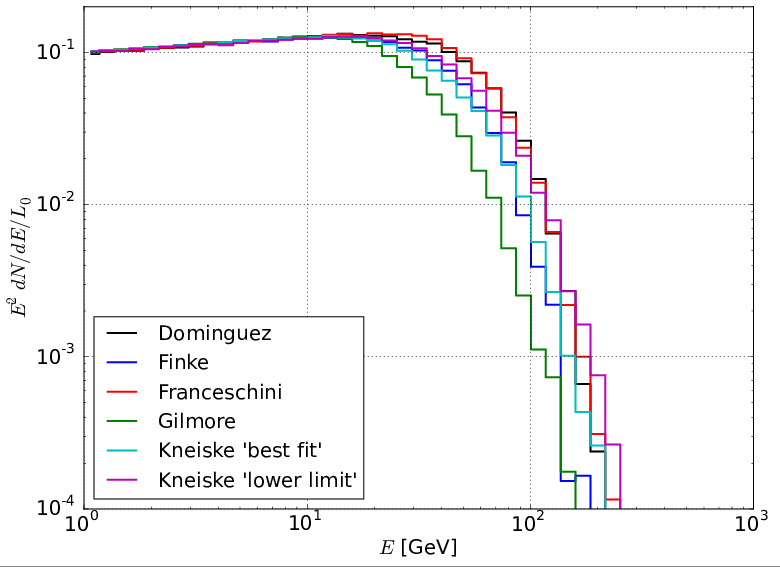
Figure 17: Full-sky spectrum for different EBL models. The source is located at redshift $z=2$.

Fig. 18 shows the distribution of detection angles for photons with energies $E>1$ GeV and for the 6 different EBL models.

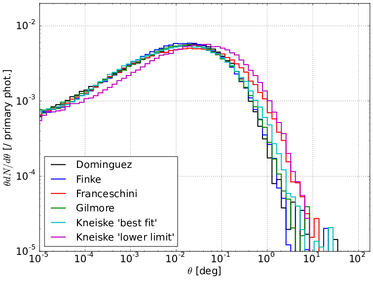
Figure 18: Detection angle distribution of $E>1$ GeV photons emitted at $z=2$ and for different EBL models.

Although the general shape of the distribution is similar from one model to the other, the typical angular scales involved can vary by a factor from 1 to 6.

5.2 Extragalactic magnetic field

The amplitude and coherence length of EGMF have no effect on the full integrated spectrum over an infinite time. It can however have an effect if the spectrum is integrated only over a finite observational time or if a limited aperture is used. These questions have already been largely studied in the literature (e.g. Taylor et al., 2011; Vovk et al., 2012; Arlen et al., 2014). We do not reproduce these studies here.

Fig. 19 shows the average time delay and arrival angle of photons with energy $E>1$ GeV versus the amplitude of the EGMF for a coherence length $\lambda_{B}=1$ Mpc.

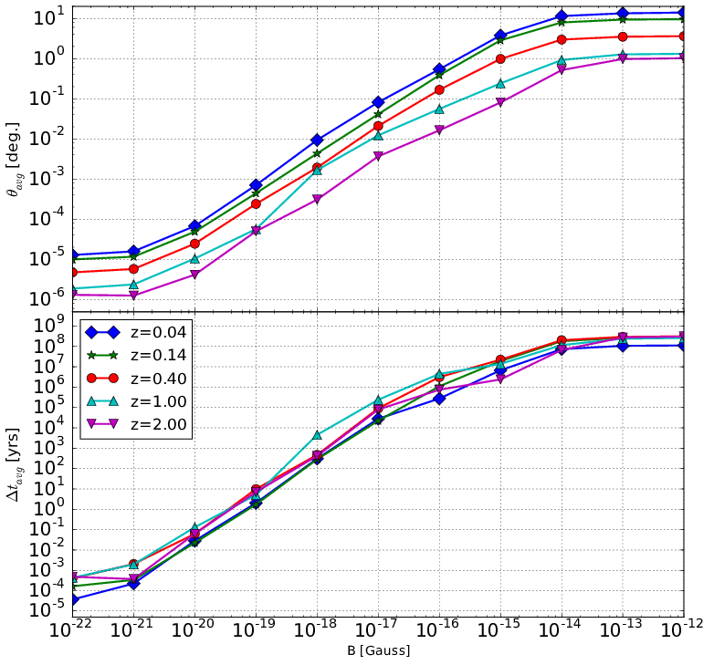
Figure 19: Average detection angle (top) and average time delay (bottom) of photons with energy $E>1$ GeV as a function of the EGMF strength for different source redshifts. The coherence length is $\lambda_{B}=1$ Mpc.

For strong magnetic fields ($B>10^{-14}$ G), leptons are trapped near their production site by the magnetic field and produce an isotropic source of typical size $\lambda_{\gamma\gamma}$. This translates into a typical average angle (and time delay), that is independent of the field intensity (Aharonian et al., 1994). For weak magnetic fields ($B<10^{-14}$G), there is no isotropisation of the emission and the average angle increases with the magnetic field intensity: the stronger the field, the larger the deflection and the larger the detection angle (Elyiv et al., 2009). For very weak magnetic fields ($B<10^{-21}$G, the arrival angle and time delay saturate at minimal values corresponding to the intrinsic extension of the cascade, resulting from the small misalignment of the product particles with respect to their parent particles during pair production and Compton interactions. This intrinsic extension is independent on the magnetic field strength (Neronov & Semikoz, 2009, Eq. 41). Also, nearby sources naturally appear as more extended than distant sources. Nonetheless, as for the effect of the jet opening angle, a combination of the intrinsic spectrum of the source and the complex absorption profile at low redshift produces an increase of the average angle that can be slower than the linear expectation of Eq. 11 and that depends on the source redshift.

The properties of the cascade emission also depend on the coherence length. The general shape of the angular and time delay distributions (not shown here) are quite insensitive to that length scale, but the typical angular (and time) scales depend on it. The average angle and time delays of photons with energy $E>1$ GeV are shown as a function of the coherence length in Fig. 20.

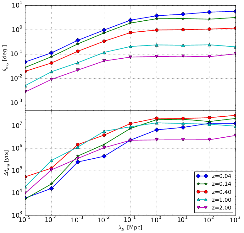
Figure 20: Average detection angle (top) and average time delay (bottom) of photons with energy $E>1$ GeV as a function of the EGMF coherence length $\lambda_{B}$ for different source redshifts. The field strength is $B=10^{-15}$ G.

At large coherence length ($\lambda_{B}>1$ Mpc), the leptons only visit a single uniform magnetic cell and the deflection is governed by the orientation of the field in that cell. This produces a halo size that is quite independent of the coherence length. At small coherence length ($\lambda_{B}<10$ kpc), the leptons travel through many magnetic cells and have a random walk. The deflection angle then increases as $\lambda_{B}^{1/2}$, and so does the detection angle. Although the angular scales cannot be derived from the simple one-generation model, the expected behaviour $\theta_{avg}\propto\lambda_{B}^{1/2}$ is well recovered by the full simulations. In the simple model presented in section 2.4, the transition between the two regimes occurs when the lepton cooling distance associated to the observation energy $E$ equals the magnetic coherence length. We consider only photons above 1 GeV and at $z=0.14$, the absorption energy is about 1 TeV. The corresponding cooling distance of the parent leptons is then in the range $10<D_{ic}<500$ kpc (according to eq. 5 and 7). The transition is then expected to occur in the same range $10<\lambda_{B}<500$ kpc as observed in Fig 20. Whereas the absorption energy depends only moderately on the source distance, the cooling distance scales as $D_{ic}\propto(1+z)^{-4}$, so that the transition occurs at much smaller coherence length for high-z sources, as observed in Fig. 20.

6 Conclusion

In this article, we have presented a new, publicly available, Monte Carlo code to model the emission of electromagnetic cascades. This code makes very few approximations: it uses the exact interaction cross sections, both the EBL and CMB photons are targets for the lepton and photon interaction, it computes the exact 3D trajectory of leptons in cubic cells immersed in an uniform magnetic field and it takes into account the cosmological expansion in the evolution of the target properties, the particle energy and the particle trajectories. It can model the emission of cascades initiated by sources at any distance (as long as EBL models are accessible), with any intrinsic spectrum and any axisymmetric emission. The code was validated by comparison to published results and analytical estimates.

With this code, we have studied the role of the different physical parameters (source spectrum, redshift, anisotropic emission, EBL spectrum and EGMF) involved in the cascade properties. This study also emphasises the limitations of the analytical estimates often used in the interpretation of high-energy observations. In particular, high-generation photons quickly dominate the cascade properties as soon as the intrinsic spectrum extends to energies significantly larger than the source absorption energy (typically a few TeV). Most studies use one-generation models to interpret the results of search for pair halos. We have shown that the angular distribution at potentially observable scales ($\theta>0.1^{\circ}$) can be fully dominated by second-generation photons if the intrinsic spectrum of the source is hard and extends to high energy. In that case, analytic expressions and their interpretations can be misleading.

The dependence of cosmological cascades on the characteristics of the sources (variability, spectrum, anisotropy) as well as those of the intergalactic medium (EBL, EGMF) is subtle and complex. Moreover, the observable properties of cascades depend also crucially on the way observations are conducted (aperture angle of the instrument, energy bands, time of the observation and time of exposure…). A detailed numerical modelling of the cascades is a prerequisite to disentangling all these effects. The code can be used: to interpret data, to design observational strategies for present and future high-energy telescopes and to tighten the constraints on the EGMF.

Appendix A Monte Carlo code

The code was designed to be accurate and general, without any approximation, fast, and easy to use. It is written in Fortran 95 and parallelised with OpenMP. The source code is available at the following address: https://gitlab.com/tfitoussi/cascade-simulation with some additional informations. Simulations return series of events (detected photons) which are then post-processed to generate observables such as spectra, angular distributions, images or timing delays. Post-processing scripts in python 2.7 are accessible at https://gitlab.com/tfitoussi/simulation-analysis. These scripts were developed for our own needs and should be considered as examples and templates. More details are given on the mentioned Git repositories.

The general architecture of the code is presented in Fig. 21 (see also section 3.1), additional details are given below on the particular way some selected physical or numerical issues are dealt with.

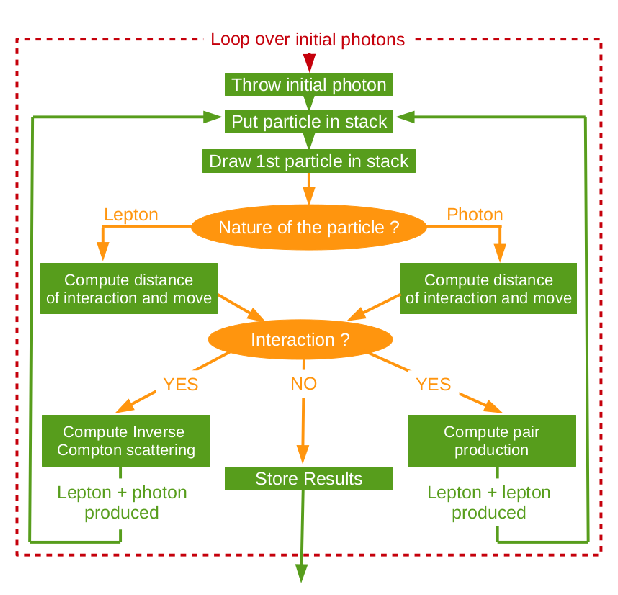
Figure 21: Scheme of the simulation process.

A.1 Particles propagation

In this section, we describe how the propagation of leptons is computed.

The Friedmann - Lemaitre - Robertson - Walker metric for a spatially flat and isotropic universe is:

$$ds^{2}=c^{2}dt^{2}-a^{2}(t)d\chi^{2},$$ (18)

where $t$ is the cosmic time, $a(t)$ is the scale factor and $\chi$ the comoving distance. The code uses a flat $\Lambda$-CDM concordance model ($\Omega_{k}=0$). The results presented in this paper have been obtained with $\Omega_{M}=0.3$, $\Omega_{\Lambda}=0.7$ and the Hubble constant $H_{0}=67.8$ km s^-1 Mpc^-1. The evolution of the Universe is described by the Friedmann - Lemaitre equation:

$$\frac{H^{2}}{H_{0}^{2}}=\left(\frac{\dot{a}}{a}\right)^{2}=\Omega_{M}(1+z)^{3}+\Omega_{k}(1+z)^{2}+\Omega_{\Lambda}$$ (19)

where $z=1/a-1$ is the cosmological redshift. Then, the evolution of redshift with cosmic time is governed by:

$$dt=\frac{da}{\dot{a}}=\frac{-dz}{(1+z)H(z)}.$$ (20)

Photons follow geodesics $ds^{2}=0$. The comoving distance travelled by photons between two interactions is therefore:

$$\Delta\chi=c\int_{t_{1}}^{t_{2}}\frac{dt}{a}=c\int_{z_{2}}^{z_{1}}\frac{dz}{H(z)}.$$ (21)

The lepton propagation is affected by the extragalactic magnetic field (EGMF) and their equation of motion is:

$$\frac{d^{2}x^{\mu}}{d\tau^{2}}+\Gamma^{\mu}_{\ \alpha\beta}\frac{dx^{\alpha}}{d\tau}\frac{dx^{\beta}}{d\tau}=\frac{f^{\mu}}{m_{e}},$$ (22)

where $m_{e}$ is the lepton mass, $x^{\mu}$ is the position quadri-vector, $\tau$ is the particle proper time, the $\Gamma^{\mu}_{\ \alpha\beta}$ are the Christofell symbols, and $f^{\mu}$ is the Lorentz force computed from the electro-magnetic tensor. We assume a passive field diluted as $B(z)=B_{0}/a^{2}$ where $B_{0}$ is its value at $z=0$. In terms of comoving coordinates $\vec{\chi}$ and cosmic time $t$, the equations of motion read:

$$\frac{d^{2}t}{d\tau^{2}}+\frac{a}{c^{2}}\frac{da}{dt}\left(\frac{d\chi}{d\tau}\right)^{2} =0,$$ (23)

$$\frac{d^{2}\vec{\chi}}{d\tau^{2}}+\frac{2}{a}\frac{da}{dt}\frac{dt}{d\tau}\frac{d\vec{\chi}}{d\tau} =\frac{e_{c}}{a^{2}m_{e}c}\frac{d\vec{\chi}}{d\tau}\times\vec{B}_{0}$$ (24)

where $e_{c}$ is the lepton charge and $c$ the speed of light. The cosmic time is linked to the particle proper time as: $d\tau=dt/\gamma$ and the comoving velocity is related to the proper velocity $v$ as: $d\chi/dt=v/ac$. Defining $p=(\gamma^{2}-1)^{1/2}$ the lepton dimensionless momentum, the first equation reduces to $\dot{p}/p=-\dot{a}/a$, the solution of which describes how the particle energy evolves with cosmic time:

$$p\propto 1/a=(1+z).$$ (25)

Note that highly relativistic particles behave very much like photons since $p\approx\gamma$. The second equation is simpler when written in terms of a generalised conformal time $\eta$ defined by $d\eta=dt/(\gamma a^{2})$:

$$\frac{d^{2}\vec{\chi}}{d\eta^{2}}+\vec{\omega}_{B,0}\times\frac{d\vec{\chi}}{d\eta}=\vec{0},$$ (26)

where $\vec{\omega}_{B,0}=e_{c}\vec{B}_{0}/(m_{e}c)$ is the cyclotron pulsation at $z=0$ (i.e. a constant). This equation is the equation of motion of a charged particle in a constant magnetic field. The solution is the classical helicoidal motion. The period of generalised conformal time between two interactions occurring at cosmic times $t_{1}$ and $t_{2}$ is computed numerically as:

$$\Delta\eta=\int_{t_{1}}^{t_{2}}\frac{dt}{\gamma a^{2}}=\int_{z_{2}}^{z_{1}}\frac{(1+z)}{\gamma(z)H(z)}dz.$$ (27)

And the associated rotation angle is:

$$\theta=-\omega_{B,0}\Delta\eta.$$ (28)

The trajectory is then easily described by Rodrigues’ rotation formulae. Let $\vec{b}=\vec{B}/B$ the direction of the magnetic field and $\vec{u}_{1}=\vec{v}_{1}/v_{1}$ the velocity direction at time $t_{1}$. Defining two orthogonal vectors in the perpendicular plane $\vec{e_{1}}=\vec{b}\times\vec{u}_{1}$ and $\vec{e_{2}}=\vec{b}\times\vec{e_{1}}$, the change in the velocity direction and in comoving position read respectively:

$$\Delta\vec{u} =\sin\theta\vec{e_{1}}+2\sin^{2}\left(\theta/2\right)\vec{e_{2}}$$ (29)

$$\frac{\Delta\vec{\chi}}{\chi_{s}} =\vec{u}_{1}+\sin\left(\theta/2\right){\rm sinc}\left(\theta/2\right)\vec{e_{1}}+\left(1-{\rm sinc}~{}\theta\right)\vec{e_{2}}$$ (30)

where $\chi_{s}=c\Delta\eta p/(1+z)$ is the curvilinear, comoving distance travelled by the lepton, and ${\rm sinc}(x)=\sin{(x)}/x$.

Integrals 21 and 27 are computed numerically using a Gauss-Legendre quadrature with 30 quadrature points allowing to reach machine precision for floats in double precision.

A.2 Accuracy

Monte Carlo simulations of electro-magnetic cascades might suffer from numerical accuracy issues when very small angles and time delays are computed. The code is run with double precision floats, with relative precision of $\sim 10^{-15}$. This provides sufficient precision to deal with realistic cascades.

The particle directions and positions are described numerically by 3D vectors. Angles are typically computed from the arccosine of the dot product of two such vectors. The relative precision on angles is then about $\sim 10^{-7}$ rad, which is far below any instrumental PSF.

Time delays are computed by comparing the arrival time of cascade photons to the arrival time of primary photons. The particle motion is computed by integrating the trajectory, including the cosmological expansion (see Sec. A.1). This implies numerical integration and iterative methods. As explained above, numerical integrations use enough quadrature points to reach machine precision as long as $z<6$. In addition, the computation of the interaction distance is performed using the Newton-Raphson method with a convergence criterium small enough to also reach machine precision. For our cosmological model, the age of the universe is $4.3\times 10^{17}$ s. The machine precision of $10^{-15}$ then allows to access time delays shorter than one hour, which is also enough for the typical integration time of realistic observations with Fermi and Cherenkov telescopes.

A.3 Acceleration methods

Although Monte Carlo simulations allow for an exact description of each particle motion and interaction, more and more particles must be tracked by the code as the cascade develops. Here we describe some aspects of numerical acceleration methods that allow for enough cascade statistics and fast computation time, with negligible effect on the cascade physics. We use three methods to reduce the computing time.

1. As leptons cool down, they end up producing Compton photons at low energy, when they are not expected to be observed because of strong sky background and low instrument sensitivity. Below some threshold energy, leptons are thus removed from the stack and are not tracked further by the code. Identically, photons that are not detected are discarded below a corresponding threshold energy. In the results presented here, we used a lepton threshold energy of $E_{\rm th}^{e}=5.56$ GeV, which corresponds to describing the cascade emission only above 100 MeV.

2. As the cascade develops, many low-energy particles are produced, providing a much better statistics at low energy. In order to increase the relative statistics at high energy, a weighted sampling is performed at each interaction, based on the energy of the involved particles. Namely, only a fraction $f_{s}=(E_{\rm out}/E_{\rm in})^{\alpha_{s}}$ of each outgoing particle is kept, where $E_{\rm out}$ and $E_{\rm in}$ are the energy of the child and parent particles respectively, and where $\alpha_{s}$ is an efficiency parameter (typically $\alpha_{s}=0.6$ for the results shown here). In order to keep track of the physical number of particles in the simulation, each particle is given a weight. And at each interaction, the weight of the particles that are not discarded by this sampling method is increased by a factor $f_{s}$. This procedure is applied both to leptons and photons.

3. As the typical Compton interaction length ($\lesssim 1$ kpc) is much shorter than the photon annihilation distance ($\gtrsim 1$ Mpc), most of the time is spent computing the motion and Compton scatterings of leptons. At low energy, leptons up-scatter a huge number of target photons to gamma-ray energies. This large number of interactions at low energy allows to perform a sampling of the Compton interactions. Namely, target photons are gathered in macro-photons consisting of $N$ physical photons (not necessary an integer number). Leptons are then considered to interact with this much sparser population of targets, which spares a significant fraction of computation time. The interaction distance, lepton energy loss and weight of the produced gamma-rays are increased accordingly with factor $N$ while the deflection angle is increased by a factor $N^{1/2}$. The size of the macro-photons is chosen such that on average a constant fraction $\eta$ of the lepton energy is typically lost during each interaction with a macro-photon: $N=\eta E_{k}/\langle\Delta E\rangle$, where $E_{k}=(\gamma-1)m_{e}c^{2}$ is the lepton kinetic energy, $\langle\Delta E\rangle=(4/3)(\gamma^{2}-1)E_{cmb}$ is the average lepton energy loss in the Thomson regime at each scattering event on CMB photons, and $E_{cmb}=2.7T_{cmb}$ is the average energy of CMB photons. We used $\eta=0.5\%$ for the results presented here. Such an interaction sampling is performed only when $N>1$, that is for leptons with kinetic energy lower than $E_{k}/(m_{e}c^{2})=(3/4)\eta m_{e}c^{2}/E_{cmb}-2$, that is about $E_{k}<1$ TeV at $z=0$. In practice, the numerical computation of the lepton energy after the up-scattering of a macro-photon can lead to negative energies for several reasons (energy dispersion around the average value, interactions with EBL photons, interactions in the Klein-Nishina regime, and overestimation of the energy variation by assuming a constant lepton energy). However, such events remain very rare given the small fraction $\eta$ chosen here, and are simply discarded. As for particle sampling, the Compton sampling increases the relative statistics at high energy, where only few photons are detected.

A.4 Modelling isotropic and anisotropic emission

A.4.1 Code outputs

Regardless of the geometrical properties of the source emission, the code is always run with primary photons emitted in a single direction $\vec{e}_{z}$. Secondary photons are detected when they cross the sphere of comoving radius equal to the comoving distance to the source. There, the following properties of each detected photon $i$ are recorded:

• Weight $w_{i}$

• Energy $E_{i}$

• Time delay $\Delta t_{i}$

• Angular position on the sphere $\vec{n}_{p,i}$. Positions are measured in a spherical system of coordinates ($\theta_{p,i}^{\rm code},\phi_{p,i}^{\rm code}$) with main axis $\vec{e}_{z}$ (as we will see, we consider only axisymmetric cascades, so that the orientation of this base around $\vec{e}_{z}$ is irrelevant).

• Angular direction $\vec{n}_{d,i}$. Directions are measured from an observer point of view in a spherical system of coordinates ($\theta_{d,i}^{\rm code},\phi_{d,i}^{\rm code}$) with main axis the position vector $\vec{n}_{p}$ and orientation defined by the direction of the primary photons $\vec{e}_{z}$.

A.4.2 Physical observables

From these outputs, the case of an isotropic source is simply modelled by means of rotations. Namely, the integration over all emission directions $\vec{n}_{e}$ with respect to the line of sight is equivalent to the integration over all detection positions in the code outputs. Hence photons detected at any position $\theta_{p}^{\rm code}$ are kept with their other properties unchanged (weight, energy, time, direction) and any distribution (e.g. energy spectrum, angular distribution of detected photon etc) can be derived.

The case of anisotropic emission is more complex to handle. Here is a short description of the method used to model any axisymmetric emission in a post-processing stage. The derivation is based on two main assumptions:

• First, it is assumed that the source emission is axisymmetric around a jet axis that makes an angle $\theta_{\rm obs}$ with respect to the line of sight i (see Fig. 4). The source emission is described by its angular distribution $dN_{e}/d\Omega_{e}$, where $d\Omega_{e}=-\sin\theta_{e}d\theta_{e}d\phi_{e}$ is the elementary solid angle and the spherical coordinates $(\theta_{e},\phi_{e}$) are defined with respect to the jet axis $\vec{n}_{\rm jet}$. The emission distribution is typically characterised by its half opening angle $\theta_{\rm jet}$. For instance, the disk profile used in Fig. 14 is a uniform angular distribution up to the jet half opening angle: $dN_{e}/d\Omega_{e}=1/(2\pi(1-\cos\theta_{\rm jet}))$ if $\theta_{e}<\theta_{\rm jet}$ and 0 otherwise.

• Second, it is assumed that the cascade initiated by a single primary photon is axisymmetric around the direction of this primary. This approximation is accurate for small magnetic coherence lengths for which many different magnetic cells with random orientations are crossed by the particles. It might become less accurate when the magnetic field is coherent over very large distances. However, our numerical simulations show that cascades initiated by unidirectional primary photons of $E_{\gamma,0}<100$ TeV, emitted at $z=0.13$ remain highly axisymmetric up to $\lambda_{B}=10$ Mpc. Although images of misaligned jets might be inaccurate above this scale, such limitation vanishes for aligned jets and isotropic emission.

The code provides the distribution of photons in a local system of coordinated based on the direction of each primary photons. To recover the total source geometry, we must transform these results to a distribution of photons in a global system of coordinates. Energy and time delay does not depend on the choice of coordinates are kept unchanged. The position of detected photons does depend on the choice of coordinates. However a given observer corresponds to one specific position so that the detection positions is a fix parameter. Hence only the direction of detected photons must be transformed carefully.

In the global frame, the direction of secondaries is best measured in a system of spherical coordinates $(\theta_{d},\phi_{d})$ with main axis the position vector $\vec{n}_{p}$ (i.e. the line of sight) and oriented with respect to the jet axis $\vec{n}_{\rm jet}$. The direction of this base is the same as the one used to measure directions in the code (hence $\theta_{d}=\theta_{d}^{\rm code}$). However, the orientation is now defined independently of the primary direction. Images are obtained by plotting the photon density in the sky plane ($\theta_{d}\sin{\phi_{d}},\theta_{d}\cos{\phi_{d}})$. In the main body of the paper, the subscript $d$ has been dropped with no ambiguity.

Because of the axisymmetric assumptions, each detected photon actually produces a (non-uniform) ring in the sky plane of the observer. Hence, the numerical result is a continuous function of $\phi_{d}$ and a discrete function of $\theta_{d}$. For an observer misaligned by an angle $\theta_{\rm obs}$ from the jet axis, the emission from photon $i$ observed at angle $\phi_{d}$ corresponds to primary light emitted with an angle $\theta_{e,i}(\phi_{d})$ away from the jet axis, and this angle is defined as:

$$\cos\theta_{e,i}=\cos\theta_{\rm obs}\cos\theta_{p,i}^{\rm code}+\sin\theta_{\rm obs}\sin\theta_{p,i}^{\rm code}\sin(\phi_{d}-\phi_{d,i}^{\rm code}).$$ (31)

Since for an anisotropic source, the emission intensity depends on that angle, the weight of each ring $i$ depends on the azimuthal angle $\phi_{d}$:

$$W_{i}(\phi_{d})=\frac{w_{i}}{2\pi}\left.\frac{dN_{e}}{d\Omega_{e}}\right|_{\theta_{e,i}}.$$ (32)

This procedure provides the number of photons detected per unit direction-solid angle and per unit position-solid angle: $d^{2}N/(d\Omega_{p}d\Omega_{d})$ at position $\theta_{p}=\theta_{\rm obs}$ and in direction $(\theta_{d},\phi_{d})$. Dividing this further by the luminosity distance $D_{L}$ of the source gives the surface brightness, that is the number of detected photons per unit detector surface and per unit direction solid angle: $dN/(dSd\Omega_{d})=dN/(d\Omega_{p}\Omega_{d})/D_{L}^{2}$.

References

- Abramowski et al. (2014) Abramowski A., et al., 2014, A&A, 562, A145
- Aharonian & Atoyan (1985) Aharonian F. A., Atoyan A. M., 1985, International Cosmic Ray Conference, 1, 301
- Aharonian et al. (1994) Aharonian F. A., Coppi P. S., Voelk H. J., 1994, ApJ, 423, L5
- Aharonian et al. (2001) Aharonian F. A., et al., 2001, A&A, 366, 746
- Aharonian et al. (2002) Aharonian F. A., Timokhin A. N., Plyasheshnikov A. V., 2002, A&A, 384, 834
- Arlen et al. (2014) Arlen T. C., Vassilev V. V., Weisgarber T., Wakely S. P., Shafi S. Y., 2014, ApJ, 796, 18
- Batista et al. (2016) Batista R. A., Saveliev A., Sigl G., Vachaspati T., 2016, arXiv:1607.00320 [astro-ph]
- Berezinskii & Smirnov (1975) Berezinskii V. S., Smirnov A. I., 1975, Ap&SS, 32, 461
- Berezinsky & Kalashev (2016) Berezinsky V., Kalashev O., 2016, Physical Review D, 94, 023007
- Caprini & Gabici (2015) Caprini C., Gabici S., 2015, Phys. Rev. D, 91, 123514
- Chen et al. (2015) Chen W., Buckley J. H., Ferrer F., 2015, Phys. Rev. Lett., 115, 211103
- D’Avezac et al. (2007) D’Avezac P., Dubus G., Giebels B., 2007, A&A, 469, 857
- Dermer et al. (2011) Dermer C. D., Cavadini M., Razzaque S., Finke J. D., Chiang J., Lott B., 2011, ApJ, 733, L21
- Domínguez et al. (2011) Domínguez A., et al., 2011, MNRAS, 410, 2556
- Durrer & Neronov (2013) Durrer R., Neronov A., 2013, A&ARv, 21, 62
- Elyiv et al. (2009) Elyiv A., Neronov A., Semikoz D., 2009, Phys. Rev. D, 80
- Essey et al. (2011) Essey W., Ando S., Kusenko A., 2011, Astroparticle Physics, 35, 135
- Eungwanichayapant & Aharonian (2009) Eungwanichayapant A., Aharonian F., 2009, International Journal of Modern Physics D, 18, 911
- Finke et al. (2010) Finke J. D., Razzaque S., Dermer C. D., 2010, AJ, 712, 238
- Finke et al. (2015) Finke J. D., Reyes L. C., Georganopoulos M., Reynolds K., Ajello M., Fegan S. J., McCann K., 2015, arXiv:1510.02485 [astro-ph]
- Franceschini et al. (2008) Franceschini A., Rodighiero G., Vaccari M., 2008, A&A, 487, 837
- Gilmore et al. (2012) Gilmore R. C., Somerville R. S., Primack J. R., Domínguez A., 2012, MNRAS, 422, 3189
- Gould & Schréder (1967) Gould R. J., Schréder G. P., 1967, Phys. Rev. Lett., 155, 1408
- Ichiki et al. (2008) Ichiki K., Inoue S., Takahashi K., 2008, ApJ, 682, 127
- Kachelrieß (2010) Kachelrieß M., 2010, in 25th Texas Symposium on Relativistic Astrophysics. p. 224
- Kachelriess et al. (2012) Kachelriess M., Ostapchenko S., Tomas R., 2012, Computer Physics Communications, 183, 1036
- Kneiske & Dole (2010) Kneiske T. M., Dole H., 2010, A&A, 515, A19
- Krawczynski et al. (2000) Krawczynski H., Coppi P. S., Maccarone T., Aharonian F. A., 2000, A&A, 353, 97
- Kronberg (1995) Kronberg P. P., 1995, Nature, 374, 404
- Long & Vachaspati (2015) Long A. J., Vachaspati T., 2015, Journal of Cosmology and Astroparticle Physics, 2015, 065
- Meyer et al. (2016) Meyer M., Conrad J., Dickinson H., 2016, The Astrophysical Journal, 827, 147
- Murase et al. (2008) Murase K., Takahashi K., Inoue S., Ichiki K., Nagataki S., 2008, ApJ, 686, L67
- Neronov & Semikoz (2007) Neronov A., Semikoz D. V., 2007, JETP Letters, 85, 473
- Neronov & Semikoz (2009) Neronov A., Semikoz D. V., 2009, Physical Review D, 80, 123012
- Neronov & Vovk (2010) Neronov A., Vovk I., 2010, Science, 328, 73
- Neronov et al. (2010) Neronov A., Semikoz D., Kachelriess M., Ostapchenko S., Elyiv A., 2010, ApJ, 719, L130
- Neronov et al. (2011) Neronov A., Semikoz D. V., Tinyakov P. G., Tkachev I. I., 2011, A&A, 526, A90
- Oikonomou et al. (2014) Oikonomou F., Murase K., Kotera K., 2014, Astronomy & Astrophysics, 568, A110
- Plaga (1995) Plaga R., 1995, Nature, 374, 430
- Prokhorov & Moraghan (2016) Prokhorov D. A., Moraghan A., 2016, Monthly Notices of the Royal Astronomical Society, 457, 2433
- Protheroe (1986) Protheroe R. J., 1986, MNRAS, 221, 769
- Roscherr & Coppi (1998) Roscherr B., Coppi P. S., 1998, in AIP Conference Proceedings. AIP Publishing, pp 760–764, doi:10.1063/1.55297
- Settimo & De Domenico (2015) Settimo M., De Domenico M., 2015, Astroparticle Physics, 62, 92
- Stecker et al. (1992) Stecker F. W., de Jager O. C., Salamon M. H., 1992, ApJ, 390, L49
- Takahashi et al. (2008) Takahashi K., Murase K., Ichiki K., Inoue S., Nagataki S., 2008, ApJ, 687, L5
- Tavecchio et al. (2009) Tavecchio F., Ghisellini G., Ghirlanda G., Costamante L., Franceschini A., 2009, MNRAS, 399, L59
- Tavecchio et al. (2010) Tavecchio F., Ghisellini G., Foschini L., Bonnoli G., Ghirlanda G., Coppi P., 2010, MNRAS, 406, L70
- Taylor et al. (2011) Taylor A. M., Vovk I., Neronov A., 2011, A&A, 529, A144
- Vovk et al. (2012) Vovk I., Taylor A. M., Semikoz D., Neronov A., 2012, ApJ, 747, L14
- Wdowczyk et al. (1972) Wdowczyk J., Tkaczyk W., Wolfendale A. W., 1972, Journal of Physics A: General Physics, 5, 1419