Quantum state transfer on distance regular spin networks with intrinsic decoherence

Abstract

By considering distance-regular graphs as spin networks, we investigate the state transfer fidelity in this class of networks. The effect of environment on the dynamics of state transfer is modeled using Milburn’s intrinsic decoherence [G. J. Milburn, Phys. Rev. A 44, 5401 (1991)]. We consider a particular type of spin Hamiltonians which are extended version of those of Christandl et al [Phys. Rev. A 71, 032312 (2005)]. It is shown that decoherence destroys perfect communication channels. Using optimal coupling strengths derived by Jafarizadeh and Sufiani [Phys. Rev. A 77, 022315 (2008)], we show that destructive effect of environment on the communication channel increases by increasing the decoherence rate, however the state transfer fidelity reaches a steady value as time approaches infinity which is independent of the decoherence rate. Moreover, it is shown that for a given decoherence rate, the fidelity of transfer decreases by increasing the distance between the sender and the receiver.

Keywords: state transfer, distance regular spin network, intrinsic decoherence, optimal fidelity

PACs Index: 03.65.Ud

1 Introduction

The transfer of a quantum state from one part of a physical unit, e.g., a qubit, to another part is a crucial ingredient for many quantum information processing (QIP) protocols [3]. In a quantum-communication protocol, the transfer of quantum data from one location $A$ to another one $B$, can be achieved by spin networks with engineered Hamiltonians for perfect state transfer (PST) and suitable coupling strengths between spins(see for instance [2] and [4]-[9]). Particularly, Christandl, et. al showed that PST over long distances can be implemented by a modulated $N$-qubit XX chain (with engineered couplings between neighborhood spins). Then, Jafarizadeh and Sufiani in [2] extended the Christandl’s work to any arbitrary distance-regular graph as spin network and showed that by choosing suitable couplings between spins, one can achieve to the unit fidelity of state transfer. Apart from these works, it could be noticed that real systems (open systems) suffer from unavoidable interactions with their environment (outside world). These unwanted interactions show up as noise in quantum information processing systems and one needs to understand and control such noise processes in order to build useful quantum information processing systems. Open quantum systems occur in a wide range of disciplines, and many tools can be employed in their study. The dynamics of open quantum systems have been studied extensively in the field of quantum optics. The main objective in this context is to describe the time evolution of an open system with a differential equation which properly describes non-unitary behavior. This description is provided by the master equation, which can be written most generally in the Lindblad form. In fact, the master equation approach describes quantum noise in continuous time using differential equations, and is the approach to quantum noise most often used by physicists.

In the state transfer scenarios , the decoherence effects of the system-environment interactions avoid us to achieve unit fidelity. Study of the influence of different kinds of noise on the fidelity of quantum state transfer has seldom considered so far. Recently, M. L. Hu, et al [10] have studied state transfer over an $N$-qubit open spin chain with intrinsic decoherence and a chin with dephasing environment[11]. By solving the corresponding master equation analyticaly, they investigated optimal state transfer and also creation and distribution of entanglement in the model of Milburn’s intrinsic decoherence. In this work, we extend their approach to any arbitrary distance regular spin network (DRSN) in order to transfer quantum data with optimal fidelity over the antipodes of these networks. In fact it is shown that, the optimal transfer fidelity depends on the spectral properties of the networks, and the desired fidelity is evaluated in terms of the polynomials associated with the networks. Moreover, a closed formula for the steady fidelity $F^{(s)}(t)$ at large enough times $t$ is given in terms of the corresponding polynomials.

The organization of the paper is as follows. In section 2, some preliminaries such as definition of distance regular networks, technique of stratification and spectral distribution for these networks are reviewed. In section $3$, the model describing interactions of spins with each others- via a distance regular network- is introduced and the Milburn’s intrinsic decoherence is employed in order to obtain the optimal fidelity of state transfer as the main result of the paper. Section $4$ is concerned with some important examples of distance regular networks where the fidelity of transfer is evaluated in each case. Paper is ended with a brief conclusion.

2 Preliminaries

2.1 Distance-regular networks and stratification

Distance-regular graphs lie in an important category of graphs which possess some useful properties. In these graphs, the adjacency matrices $A_{i}$ are defined based on shortest path distance denoted by $\partial$. More clearly, if $\partial(\alpha,\beta)$ (distance between the nodes $\alpha,\beta\in V$) be the length of the shortest walk connecting $\alpha$ and $\beta$ (recall that a finite sequence $\alpha_{0},\alpha_{1},...,\alpha_{n}\in V$ is called a walk of length $n$ if $\alpha_{k-1}\sim\alpha_{k}$ for all $k=1,2,...,n$, where $\alpha_{k-1}\sim\alpha_{k}$ means that $\alpha_{k-1}$ is adjacent with $\alpha_{k}$), then the adjacency matrices $A_{i}$ for $i=0,1,...,d$ in distance-regular graphs are defined as: $(A_{i})_{\alpha,\beta}=1$ if and only if $\partial(\alpha,\beta)=i$ and $(A_{i})_{\alpha,\beta}=0$ otherwise, where $d:=$max$\{\partial(\alpha,\beta):\alpha,\beta\in V\}$ is called the diameter of the graph. In fact, an undirected connected graph $G=(V,E)$ is called distance-regular graph (DRG) with diameter $d$ if for all $i,j,k\in\{0,1,...,d\}$, and $\alpha,\beta$ with $\partial(\alpha,\beta)=k$, the number

$$p^{k}_{ij}=\mid\{\gamma\in V:\partial(\alpha,\gamma)=i\;\ and\;\ \partial(\gamma,\beta)=j\}\mid$$ (2-1)

is constant in that it depends only on $k,i,j$ but does not depend on the choice of $\alpha$ and $\beta$. Some more details about these graphs have been given in the section $B.I$ of the Appendix $B$ of Ref.[2].

For a given vertex $\alpha\in V$, let $\Gamma_{i}(\alpha):=\{\beta\in V:\partial(\alpha,\beta)=i\}$ denotes the set of all vertices being at distance $i$ from $\alpha$. Then, the vertex set $V$ can be written as disjoint union of $\Gamma_{i}(\alpha)$ for $i=0,1,2,...,d$, i.e.,

$$V=\bigcup_{i=0}^{d}\Gamma_{i}(\alpha),$$ (2-2)

In fact, by fixing a point $o\in V$ as a reference vertex, the relation (2-2) stratifies the vertices into a disjoint union of associate classes $\Gamma_{i}(o)$ (called the $i$-th stratum or $i$-th column with respect to $o$). With each associate class $\Gamma_{i}(o)$ we associate a normalized vector in $l^{2}(V)$ (the Hilbert space of all square summable functions in $V$) defined by

$$|\phi_{i}\rangle=\frac{1}{\sqrt{\kappa_{i}}}\sum_{\alpha\in\Gamma_{i}(o)}|\alpha\rangle,$$ (2-3)

where, $|\alpha\rangle$ denotes the eigenket of $\alpha$-th vertex at the associate class $\Gamma_{i}(o)$ and $\kappa_{i}=|\Gamma_{i}(o)|$ is called the $i$-th valency of the graph. The space spanned by $|\phi_{i}\rangle$s, for $i=0,1,...,d$ is called “stratification space”. Then, the adjacency matrix reduced to this space satisfies the following three term recursion relation

$$A|\phi_{i}\rangle=\beta_{i+1}|\phi_{i+1}\rangle+\alpha_{i}|\phi_{i}\rangle+\beta_{i}|\phi_{i-1}\rangle.$$ (2-4)

i.e., the adjacency matrix $A$ takes a tridiagonal form in the orthonormal bases $\{|\phi_{i}\rangle,i=0,1,\ldots,d-1\}$, so that, for spin networks of distance-regular type we can restrict our attention to the stratification space for the purpose of state transfer from $|\phi_{0}\rangle$ to $|\phi_{d}\rangle$ (state associated with the last stratum of the network). For the purpose of optimal state transfer, we will deal with particular distance-regular graphs (as spin networks) for which starting from an arbitrary vertex as reference vertex (prepared in the initial state which we wish to transfer), the last stratum of the networks with respect to the reference state contains only one vertex.

Now, let $A_{i}$ be the $i$th adjacency matrix of the graph $\Gamma=(V,E)$. Then, for the reference state $|\phi_{0}\rangle=|o\rangle$ one can write

$$A_{i}|\phi_{0}\rangle=\sum_{\beta\in\Gamma_{i}(o)}|\beta\rangle.$$ (2-5)

Then, by using (2-3) and (2-5), we obtain

$$A_{i}|\phi_{0}\rangle=\sqrt{\kappa_{i}}|\phi_{i}\rangle.$$ (2-6)

It can be shown that [2], for the adjacency matrices $A_{i}$ of distence regular graphs, we have

$$A_{i}=P_{i}(A),\;\ i=0,1,...,d,$$ (2-7)

where, $P_{i}$ is a polynomial of degree $i$. Then, the Eq.(2-6) gives

$$|\phi_{i}\rangle=\frac{P_{i}(A)}{\sqrt{\kappa_{i}}}|\phi_{0}\rangle.$$ (2-8)

2.2 Spectral techniques

In this subsection, we recall some preliminary facts about spectral techniques used in the paper, where more details have been given in the appendix $B.II$ of [2] and Refs. [12]-[15].

Actually the spectral analysis of operators is an important issue in quantum mechanics, operator theory and mathematical physics [16, 17]. As an example $\mu(dx)=|\psi(x)|^{2}dx$ ($\mu(dp)=|\widetilde{\psi}(p)|^{2}dp$) is a spectral distribution which is assigned to the position (momentum) operator $\hat{X}(\hat{P})$.

It is well known that, for any pair $(A,|\phi_{0}\rangle)$ of a matrix $A$ and a vector $|\phi_{0}\rangle$, one can assign a measure $\mu$ as follows

$$\mu(x)=\langle\phi_{0}|E(x)|\phi_{0}\rangle,$$ (2-9)

where $E(x)=\sum_{i}|u_{i}\rangle\langle u_{i}|$ is the operator of projection onto the eigenspace of $A$ corresponding to eigenvalue $x$, i.e.,

$$A=\int xE(x)dx.$$ (2-10)

Then, for any polynomial $P(A)$ we have

$$P(A)=\int P(x)E(x)dx,$$ (2-11)

where for discrete spectrum the above integrals are replaced by summation. Therefore, using the relations (2-9) and (2-11), the expectation value of powers of adjacency matrix $A$ over reference vector $|\phi_{0}\rangle$ can be written as

$$\langle\phi_{0}|A^{m}|\phi_{0}\rangle=\int_{R}x^{m}\mu(dx),\;\;\;\;\ m=0,1,2,....$$ (2-12)

Obviously, the relation (2-12) implies an isomorphism from the Hilbert space of the stratification onto the closed linear span of the orthogonal polynomials with respect to the measure $\mu$. Moreover, using the correspondence $A\equiv x$ and the equations (2-4) and (2-8), one gets three term recursion relations between polynomials $P_{i}(x)$

$$\beta_{i+1}\frac{P_{i+1}(x)}{\sqrt{\kappa_{i+1}}}=(x-\alpha_{i})\frac{P_{i}(x)}{\sqrt{\kappa_{i}}}-\beta_{i}\frac{P_{i-1}(x)}{\sqrt{\kappa_{i-1}}}$$ (2-13)

for $i=0,...,d-1$. Multiplying by $\beta_{1}...\beta_{i}$ we obtain

$$\beta_{1}...\beta_{i+1}\frac{P_{i+1}(x)}{\sqrt{\kappa_{i+1}}}=(x-\alpha_{i})\beta_{1}...\beta_{i}\frac{P_{i}(x)}{\sqrt{\kappa_{i}}}-\beta_{i}^{2}.\beta_{1}...\beta_{i-1}\frac{P_{i-1}(x)}{\sqrt{\kappa_{i-1}}}.$$ (2-14)

By rescaling $P_{i}$ as $Q_{i}=\beta_{1}...\beta_{i}\frac{P_{i}}{\sqrt{\kappa_{i}}}$, the three term recursion relations (2-13) are replaced by

$$Q_{0}(x)=1,\;\;\;\;\;\ Q_{1}(x)=x,$$

$$Q_{i+1}(x)=(x-\alpha_{i})Q_{i}(x)-\beta_{i}^{2}Q_{i-1}(x),$$ (2-15)

for $i=1,2,...,d$.

In the next section, we will need the distinct eigenvalues of adjacency matrix of a given undirected graph and the corresponding eigenvectors in order to obtain the evolved density matrix and the corresponding fidelity of state transfer. As it is known from spectral theory, we have the eigenvalues $x_{k}$ of the adjacency matrix $A$ as roots of the last polynomial $Q_{d+1}(x)$ in (2-15), and the normalized eigenvectors as [22, 23]

$$|\psi_{k}\rangle=\frac{1}{\sqrt{\sum_{l=0}^{d}P^{2}_{l}(x_{k})}}\left(\begin{array}[]{c}P_{0}(x_{k})\\ P_{1}(x_{k})\\ \vdots\\ P_{d}(x_{k})\\ \end{array}\right),$$ (2-16)

in which we have $P_{i}(x)={\frac{\sqrt{\kappa_{i}}}{\beta_{1}\ldots\beta_{i}}}Q_{i}(x)$ for $i=0,1,\ldots,d$.

3 The model

The model we will consider is a distance-regular network consisting of $N$ sites labeled by $\{1,2,...,N\}$ and diameter $d$. Then we stratify the network with respect to a chosen reference site, say $1$, and assume that the network contains only the output site $N$ in its last stratum (i.e., $|\phi_{d}\rangle=|N\rangle$). At time $t=0$, the qubit in the first (input) site of the network is prepared in the state $|\psi_{in}\rangle$. We wish to transfer the state to the $N$th (output) site of the network with unit efficiency after a well-defined period of time. Although our qubits represent generic two state systems, for the convenience of exposition we will use the term spin as it provides a simple physical picture of the network. The standard basis for an individual qubit is chosen to be $\{|0\rangle=|\downarrow\rangle,\;\ |1\rangle=|\uparrow\rangle\}$, and we shall assume that initially all spins point “down” along a prescribed $z$ axis; i.e., the network is in the state $|\b{0}\rangle=|0_{A}00...00_{B}\rangle$. Then, we consider the dynamics of the system to be governed by the quantum-mechanical Hamiltonian

$$H_{G}=\frac{1}{2}\sum_{m=0}^{d}J_{m}\sum_{{}_{(i,j)\in R_{m}}}H_{ij},$$ (3-17)

with $H_{ij}$ as

$$H_{ij}={\mathbf{\sigma}}_{i}\cdot{\mathbf{\sigma}}_{j},$$ (3-18)

where, ${\mathbf{\sigma}}_{i}$ is a vector with familiar Pauli matrices $\sigma^{x}_{i},\sigma^{y}_{i}$ and $\sigma^{z}_{i}$ as its components acting on the one-site Hilbert space ${\mathcal{H}}_{i}$, and $J_{m}$ is the coupling strength between the reference site $1$ and all of the sites belonging to the $m$-th stratum with respect to $1$.

Then, by employing the symmetry corresponding to conservation of $z$ component of the total spin and reduction of the main Hilbert space to the single excitation subspace spanned by the basis $\{|l\rangle,l=1,\ldots,N\}$ with $|l\rangle=|0...0\underbrace{1}_{l-th}0...0\rangle$, the hamiltonian in (3-17) can be written in terms of the adjacency matrices $A_{i}$, $i=0,1,...,d$ as follows

$$H=2\sum_{m=0}^{d}J_{m}A_{m}+\frac{N-4}{2}\sum_{m=0}^{d}J_{m}\kappa_{m}I.$$ (3-19)

For details, see [2]. For the purpose of the optimal transfer of state, as we will see in the next subsection, we will need only the difference between the energies, and so the second constant term in (3-19) dose not affect the last desired result and can be neglected for simplicity.

Now, using the Eq.(2-7) and restricting the $N$-dimensional single excitation subspace to the $(d+1)$-dimensional Krylov subspace spanned by the stratification basis $\{|\phi_{0}\rangle,|\phi_{1}\rangle,\ldots,|\phi_{d-1}\rangle\}$, we can write

$$H=2\sum_{m=0}^{d}J_{m}P_{m}(A)=2\sum_{m=0}^{d}J_{m}\sum_{k=0}^{d}P_{m}(x_{k})|\psi_{k}\rangle\langle\psi_{k^{\prime}}|,$$ (3-20)

where $x_{k}$ and $|\psi_{k}\rangle$ for $k=0,1,\ldots,d$ are the corresponding eigenvalues and eigenvectors of the adjacency matrix $A$ given by the spectral method illustrated in the previous sections (given by Eq.(2-16)). Obviously, the energy eigenvalues are given by

$$E_{k}=2\sum_{m=0}^{d}J_{m}P_{m}(x_{k}).$$ (3-21)

3.1 Milburn’s intrinsic decoherence

Milburn in ref. [1] has assumed that on sufficiently short time steps, the system does not evolve continuously under unitary evolution but rather in a stochastic sequence of identical unitary transformations which can account for the disappearance of quantum coherence as the system evolves. With this assumption, Milburn obtained the master equation for the evolution of the system as

$$\frac{d\rho}{dt}=\frac{1}{\gamma}\{\exp(-i\gamma H)\rho\exp(i\gamma H)-\rho\},$$ (3-22)

where $\gamma$ is the intrinsic decoherence parameter and $H$ is the Hamiltonian of the considered system. Expanding the above equation, keeping terms up to first order in $\gamma$ gives

$$\frac{d\rho}{dt}=-i[H,\rho]-\frac{\gamma}{2}[H,[H,\rho]].$$ (3-23)

The second term on the r.h.s of the above equation represents the decoherence effect on the system, where in the limit of $\gamma\rightarrow 0$ the ordinary Schrödinger equation is recovered. By defining three auxiliary super-operators $J$, $S$ and $L$ as

$$J\rho=\gamma H\rho H,\;\;\ S\rho=-i[H,\rho],\;\;\ L\rho=-\frac{\gamma}{2}\{H^{2},\rho\},$$

one can straightforwardly show that [10] the Eq.(3-23) simplifies to ${\frac{d\rho}{dt}}=(J+S+L)\rho$, where its solution can be written in terms of the so called Kraus operators $K_{l}(t)$ as

$$\rho(t)=\sum^{{\infty}}_{{}_{l=0}}K_{l}(t)\rho(0)K^{{{\dagger}}}_{l}(t).$$ (3-24)

In the Eq.(3-24), $\rho(0)$ denotes the initial state of the system and the Kraus operators $K_{l}(t)=(\gamma t)^{l/2}H^{l}\exp(-iHt)\exp(-\gamma tH^{2}/2)/\sqrt{l!}$ satisfy the relation $\sum^{{\infty}}_{l=0}K^{{{\dagger}}}_{l}(t)K_{l}(t)=I$ for all times $t$.

Now by expanding $\rho(0)$ in terms of energy eigenstates as $\rho(0)=\sum_{k,k^{\prime}}a_{kk^{\prime}}|\psi_{k}\rangle\langle{\psi_{k^{\prime}}}|$, one can obtain

$$\rho(t)=\sum_{k,k^{\prime}}a_{kk^{\prime}}\exp[-it(E_{k}-E_{k^{\prime}})-\frac{\gamma t}{2}(E_{k}-E_{k^{\prime}})^{2}]|\psi_{k}\rangle\langle\psi_{k^{\prime}}|$$ (3-25)

where $a_{kk^{\prime}}=\langle\psi_{k}|\rho(0)|\psi_{k^{\prime}}\rangle$, $E_{k}$ and $|\psi_{k}\rangle$ are eigenvalues and the corresponding eigenvectors of the system. Consider the initial state as

$$\rho(0)=|{\phi_{0}}\rangle\langle{\phi_{0}}|=\sum a_{kk^{\prime}}|{\psi_{k}}\rangle\langle{\psi_{k^{\prime}}}|,$$

where, using Eq.(2-16), we have

$$a_{kk^{\prime}}=\langle{\psi_{k}}|{\phi_{0}}\rangle\langle{\phi_{0}}|{\psi_{k^{\prime}}}\rangle=\frac{P_{0}(x_{k})P_{0}(x_{k^{\prime}})}{\sqrt{\sum_{l}{P_{l}}^{2}(x_{k})\sum_{l}{P_{l}}^{2}(x_{k^{\prime}})}}=\frac{1}{\sqrt{\sum_{l}{P_{l}}^{2}(x_{k})\sum_{l}{P_{l}}^{2}(x_{k^{\prime}})}}.$$

Then, Eq.(3-25) gives us

$$\rho(t)=\sum_{k,k^{\prime}}{\frac{\exp{[-it(E_{k}-E_{k^{\prime}})-\frac{\gamma t}{2}(E_{k}-E_{k^{\prime}})^{2}]}}{\sqrt{\sum_{l}{P_{l}}^{2}(x_{k})\sum_{l}{P_{l}}^{2}(x_{k^{\prime}})}}}|\psi_{k}\rangle\langle\psi_{k^{\prime}}|.$$ (3-26)

Now, employing the Eq.(2-16), the fidelity of state transfer is given by

$$F(t)=\langle{\phi_{d}}|\rho(t)|{\phi_{d}}\rangle=\sum_{k,k^{\prime}}\frac{\exp[-it(E_{k}-E_{k^{\prime}})-\frac{\gamma t}{2}(E_{k}-E_{k^{\prime}})^{2}]}{{\sum_{l}{P_{l}}^{2}(x_{k})\sum_{l}{P_{l}}^{2}(x_{k^{\prime}})}}P_{d}(x_{k})P_{d}(x_{k^{\prime}}),$$ (3-27)

where the eigenvalues $E_{k}$ are evaluated via the Eq. (3-21). On the other hands, one can show that for distance regular networks, we have $P_{d}(x_{k})=(-1)^{k}$ (see Refs. [19], [20]). Therefore the fidelity (3-27) is simplified to

$$F(t)=\langle{\phi_{d}}|\rho(t)|{\phi_{d}}\rangle=\sum_{k,k^{\prime}}(-1)^{k+k^{\prime}}\frac{\exp[-it(E_{k}-E_{k^{\prime}})-\frac{\gamma t}{2}(E_{k}-E_{k^{\prime}})^{2}]}{{\sum_{l}{P_{l}}^{2}(x_{k})\sum_{l}{P_{l}}^{2}(x_{k^{\prime}})}}.$$ (3-28)

Due to the exponential term in the Eq.(3-27), for large enough times $t\rightarrow{\infty}$ the transfer fidelity tends to zero except for $k$,$k^{\prime}$ with $E_{k}=E_{k^{\prime}}$. Therefore, after large enough times $t\gg$, the transfer fidelity arrives at a stable value as follows

$$F^{s}(t\rightarrow\infty)=\sum_{k=0}^{d}\frac{1}{[\sum_{l}{P_{l}}^{2}(x_{k})]^{2}}+2\sum_{{k<k^{\prime}}_{with{E_{k}=E_{k^{\prime}}}}}^{d}\frac{(-1)^{k+k^{\prime}}}{\sum_{l}{P_{l}}^{2}(x_{k})\sum_{l}{P_{l}}^{2}(x_{k^{\prime}})}.$$ (3-29)

In fact for the networks for which $E_{k}\neq E_{k^{\prime}}$ for $k\neq k^{\prime}$, one obtains the steady fidelity as

$$F^{s}(t\rightarrow\infty)=\sum_{k=0}^{d}\frac{1}{[\sum_{l}{P_{l}}^{2}(x_{k})]^{2}}=\sum_{k=0}^{d}a^{2}_{kk}.$$ (3-30)

4 Examples

4.1 The Cyclic network with even number of nodes

A well known example of distance-regular networks, is the cycle graph with $N$ vertices denoted by $C_{N}$. For the purpose of optimal state transfer, we consider the even number of vertices $N=2m$ for which the last stratum contains a single state corresponding to the $m$-th node. The adjacency matrices are given by

$$A_{0}=I_{2m},\;\;\ A_{i}=S^{i}+S^{-i},\;\ i=1,2,...,m-1,\;\;\ A_{m}=S^{m},$$ (4-31)

where, $S$ is the $N\times N$ circulant matrix with period $N$ (i.e. $S^{N}=I_{N}$). The corresponding parameters $\alpha_{i}$ and $\beta_{i}$ are given by

$$\alpha_{i}=0,\;\ i=0,1,...,m;\;\ \beta_{1}=\beta_{m}=\sqrt{2},\;\ \beta_{i}=1,\;\ i=2,...,m-1.$$ (4-32)

Now, using the recursion relations (2-15), one can show that

$$Q_{0}(x)=P_{0}(x)=1,\;\ Q_{i}(x)=P_{i}(x)=2T_{i}(x/2),\;\ i=1,...,m-1,\;\;\ Q_{m}(x)=2P_{m}(x)=2T_{m}(x/2),$$ (4-33)

where $T_{i}$’s are Tchebychev polynomials of the first kind. Then, the eigenvalues of the adjacency matrix $A\equiv A_{1}$ are given by

$$x_{i}=\omega^{i}+\omega^{-i}=2\cos(2\pi i/N)=2\cos(\pi i/m),\;\ i=0,1,...,m$$

with $\omega:=e^{2\pi i/N}$. Details have given in Ref.[2].

By choosing the suitable coupling constants given in [3], and Eq. (3-28), the fidelity of transfer can be plotted. In Figure 1, the fidelity of transfer has plotted for $N=4$ with three different decoherence rates $\gamma=0.1$, $\gamma=0.2$ and $\gamma=0.3$ and coupling constants $J_{0}=-J_{2}=-\pi/4$ and $J_{1}=0$. Figure 2 shows the fidelity of transfer for the cases $N=4$, $N=6$ and $N=8$ with $\gamma=0.1$ and the same coupling strengths. As it is seen from Figure 1 and Figure 2, the fidelity decreases with increasing decoherence rate $\gamma$; and for a given $\gamma$, the optimal probability of transfer decreases by distance.

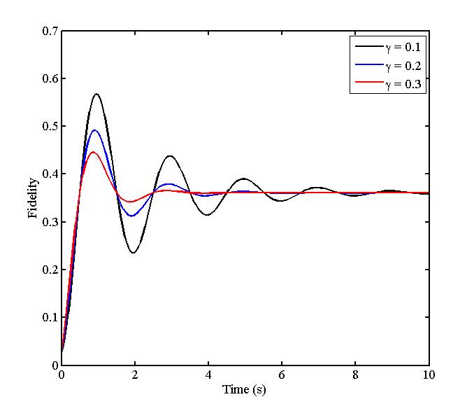
Figure 1: (Color online) Dynamics of the state transfer fidelity for $C_{4}$ with three different decoherence rates

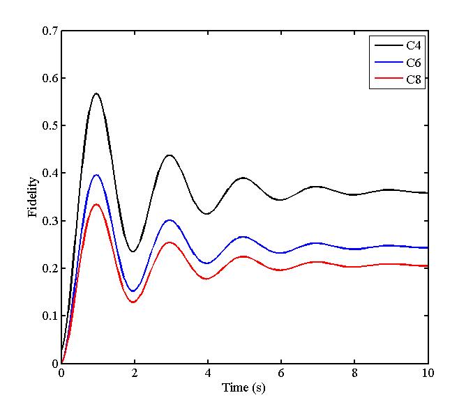
Figure 2: (Color online) Dynamics of the state transfer fidelity for $C_{N}$ with $N=4,6,8$ and $\gamma=0.1$

4.2 The hypercube network

The hypercube of dimension $d$ (known also as binary Hamming scheme $H(d,2)$) is a network with $N=2^{d}$ nodes, each of which can be labeled by an $d$-bit binary string. Two nodes on the hypercube described by bitstrings $\vec{x}$ and $\vec{y}$ are are connected by an edge if $|\vec{x}-\vec{y}|=1$, where $|\vec{x}|$ is the Hamming weight of $\vec{x}$.

In other words, if $\vec{x}$ and $\vec{y}$ differ by only a single bit flip, then the two corresponding nodes on the network are connected. Thus, each of $2^{d}$ nodes on the hypercube has degree $d$. For the hypercube network with dimension $d$ we have $d+1$ strata with adjacency matrices

$$A_{i}=\sum_{perm.}\underbrace{\sigma_{x}\otimes\sigma_{x}...\otimes\sigma_{x}}_{i}\underbrace{\otimes I_{2}\otimes...\otimes I_{2}}_{d-i},\;\ i=0,1,...,d,$$ (4-34)

where, the summation is taken over all possible nontrivial permutations. The eigenvalues $x_{i}$ and the corresponding parameters $\alpha_{i}$ and $\beta_{i}$ for $i=0,1,...,d$, are given by $x_{i}=2i-d$ and

$$\alpha_{i}=0,\;\;\ \beta_{i}=\sqrt{i(d-i+1)},$$

respectively. For details see Ref.[2]. Figure 3 shows the optimal fidelity of transfer for the case $d=3$(the known cube network) with decoherence rates $\gamma=0.1$, $\gamma=0.2$ and $\gamma=0.3$. We have chosen the optimal set of coupling strengths $J_{0}=-\frac{3\pi}{4},\;\ J_{1}=\frac{\pi}{4},\;\ J_{2}=J_{3}=0$ given in Ref.[2]. In Figure 4, the results for the cases $d=3$, $d=4$ and $d=5$ is shown, where it is seen that the fidelity decreases by increasing the dimension $d$ of the hypercube $H(d,2)$.

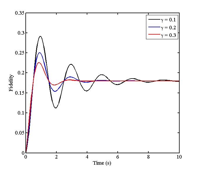
Figure 3: (Color online) Dynamics of the state transfer fidelity for the cube network $H(3,2)$ with three different decoherence rates

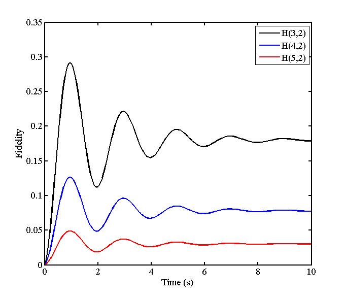
Figure 4: (Color online) Dynamics of the state transfer fidelity for $H(d,2)$ with $d=3,4,5$ and $\gamma=0.1$

4.3 The Crown network

A crown graph on $2m$ vertices is an undirected network with two sets of vertices $u_{i}$ and $v_{i}$, where the vertex $u_{i}$ is connected to $v_{j}$ whenever $i\neq j$. The corresponding adjacency matrix is given by $A=K_{m}\otimes\sigma_{x}$ where, $K_{m}$ is the adjacency matrix of the complete graph with $m$ vertices and $\sigma_{x}$ is the Pauli matrix. Then, the stratification bases (Krylov bases) are given by

$$|\phi_{0}\rangle=|1\rangle,$$

$$|\phi_{1}\rangle=\frac{1}{\sqrt{n-1}}(|m+1\rangle+|m+2\rangle+\cdots+|2m-1\rangle),$$

$$|\phi_{2}\rangle=\frac{1}{\sqrt{m-1}}(|2\rangle+|3\rangle+\cdots+|m\rangle),$$

$$|\phi_{3}\rangle=|2m\rangle.$$

In the $\{|\phi_{i}\rangle\}$ bases, the adjacency matrix is represented as

$$A=\left(\begin{array}[]{cccc}0&\sqrt{m-1}&0&0\\ \sqrt{m-1}&0&m-2&0\\ 0&m-2&0&\sqrt{m-1}\\ 0&0&\sqrt{m-1}&0\\ \end{array}\right),$$

so that we have $\alpha_{i}=0$ for $i=0,1,2,3$ and $\beta_{1}=\beta_{3}=\sqrt{m-1},\;\ \beta_{2}=m-2$. Now, by using (2-15) one can easily calculate the roots $x_{i}$ as follows:

$$x_{0}=-(m-1),\;\ x_{1}=-1,\;\ x_{2}=1,\;\ x_{3}=(m-1).$$

Now, following the algorithm given in [2], one can obtain the optimal couplings $J_{i}$ as follows

$$J_{0}=-\frac{\pi}{4},\;\;\ J_{1}=J_{2}=0,\;\;\ J_{3}=\frac{\pi}{4}.$$

Figure 5 shows the optimal fidelity of transfer for the case $m=3$ with decoherence rates $\gamma=0.1$, $\gamma=0.2$ and $\gamma=0.3$. Plots for the cases $m=3$, $m=4$ and $m=5$ with $\gamma=0.1$ are shown in Figure 6.

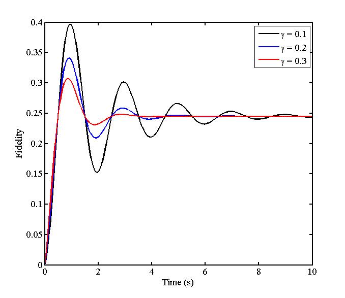
Figure 5: (Color online) Dynamics of the state transfer fidelity for the Crown network with $m=3$ and three different decoherence rates

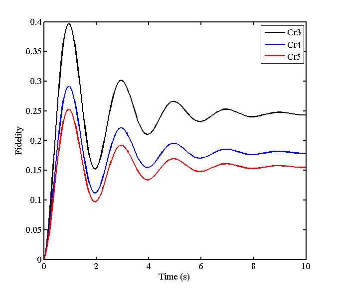
Figure 6: (Color online) Dynamics of the state transfer fidelity for the Crown network with $m=3,4,5$ and $\gamma=0.1$

5 Conclusion

In summery, optimal state transfer over distance regular spin networks (DRSN) in the Milburn’s intrinsic decoherence environment was studied. In fact, using the spectral properties of these networks and employing the stratification technique for them, we obtained the transfer fidelity over DRSNs in terms of the polynomials associated with them. By choosing the optimal coupling constants (considered in Phys. Rev. A 77, 022315 (2008)) for perfect state transfer (PST), it was seen that intrinsic decoherence destroys perfect communication so that destructive effect of environment on the communication channel increases by increasing the decoherence rate. However the transfer fidelity reaches a steady value as time approaches infinity which is independent of the decoherence rate. Moreover, it was shown in some examples that for a given decoherence rate, the fidelity of transfer decreases by distance between the sender and the receiver (antipodes of the corresponding networks).

References

- [1] G. J. Milburn, Phys. Rev. A 44, 5401 (1991).
- [2] M. A. Jafarizadeh and R. Sufiani, Phys. Rev. A 77, 022315, (2008).
- [3] D. Bouwmeester, A. Ekert, and A. Zeilinger, (2000), The Physics of Quantum Information (Springer-Verlag, Berlin).
- [4] S. Bose, (2003), Phys. Rev. Lett. 91, 207901.
- [5] M. Christandl, N. Datta, A. Ekert, and A. J. Landahl, (2004), Phys. Rev. Lett. 92, 187902.
- [6] M. Christandl, N. Datta, T. C. Dorlas, A. Ekert, A. Kay and A. J. Landahl, (2005), Phys. Rev. A 71, 032312.
- [7] D. Burgarth, S. Bose, Phys.Rev.A 71, 052315(2005).
- [8] R. H. Crooks, D.V. khveshchenko, Phys.Rev. A 77,062305 (2008).
- [9] V. Kostak, G. M. Nikolopoulos, I. Jex, Phys. Rev. A 75, 042319 (2007).
- [10] Hu, M. and Lian, H. Eur. Phys. J. D (2009) 55: 711. doi:10.1140/epjd/e2009-00220-8.
- [11] Hu, M. and Lian, H. Eur. Phys. J. D (2011) 59 (3). doi:10.1140/epjd/e2010-001837.
- [12] M. A. Jafarizadeh and S. Salimi,(2006), J. Phys. A : Math. Gen. 39, 1-29.
- [13] M. A. Jafarizadeh, R. Sufiani, S. Salimi and S. Jafarizadeh, (2007), Eur. Phys. J. B 59, 199-216.
- [14] M. A. Jafarizadeh, R. Sufiani and S. Jafarizadeh, (2007), J. Phys. A: Math. Theor. 40, 4949-4972.
- [15] M. A. Jafarizadeh, S. Salimi, (2007), Annals of physics, Vol. 322 1005-1033.
- [16] H. Cycon, R. Forese, W. Kirsch and B. Simon Schrodinger operators (Springer-Verlag, 1987).
- [17] P. D. Hislop and I. M. Sigal, Introduction to spectral theory: With applications to schrodinger operators (1995).
- [18] M. A. Jafarizadeh, et al., J. Phys. A: Math. Theor. 41, 475302, (2008).
- [19] G. Coutinho, et. al, Perfect state transfer on distance-regular graphs and association schemes, quant-ph/14011745, (2014).
- [20] A. E. Brouwer and W. H. Haemers. Spectra of graphs. Universitext. Springer, New York, 2012.
- [21] M A Jafarizadeh, et al., J. Stat. Mech. 05014, (2011).
- [22] T. S. Chihara, An Introduction to Orthogonal Polynomials, Gordon and Breach, Science Publishers Inc, 1978.
- [23] Z. Alipour, M.A. Jafarizadeh, N. Fooladi and R. Sufiani, International Journal of Modern Physics E, 1465-1476, 2011.
- [24] Turchette,Q.A., Hood,C.J., Lange,W., Mabuchi,H., Kimble,H.J., Phys. Rev. Lett. 75, 4710 (1995); M. Brune et al., Phys. Rev. Lett. 77, 4887 (1996).
- [25] Mattle,K., Weinfurter,H., Kwiat,P.G., Zeilinger,A., Phys. Rev. Lett. 76, 4656 (1996).