A Simulation Tool for tccp Programs

Abstract

The Timed Concurrent Constraint Language tccp is a declarative synchronous concurrent language, particularly suitable for modelling reactive systems. In tccp, agents communicate and synchronise through a global constraint store. It supports a notion of discrete time that allows all non-blocked agents to proceed with their execution simultaneously.

In this paper, we present a modular architecture for the simulation of tccp programs. The tool comprises three main components. First, a set of basic abstract instructions able to model the tccp agent behaviour, the memory model needed to manage the active agents and the state of the store during the execution. Second, the agent interpreter that executes the instructions of the current agent iteratively and calculates the new agents to be executed at the next time instant. Finally, the constraint solver components which are the modules that deal with constraints.

In this paper, we describe the implementation of these components and present an example of a real system modelled in tccp.

Section 1 Introduction

It is well known that many critical applications in different domains, such as health [26], railways [22] or automotive [17] have a reactive and concurrent behaviour that is difficult to model and analyse. Unfortunately, certain errors in these applications may have highly negative consequences and, therefore, it is essential to detect failures in software in the early design phases. This is why most modelling languages for these complex systems are supported by simulation and verification tools that guarantee the software’s safety and reliability with respect to the critical properties.

Several formalisms have been developed to solve the problem of describing and analysing concurrent systems. In this paper, we focus on the Concurrent Constraint Paradigm (ccp) [23] characterised by the use of store-as-constraint instead of the classical store-as-value paradigm. Specifically, tccp [7] is a language suitable for describing reactive systems within this paradigm. As opposed to the interleaving composition of processes supported by most concurrent modelling languages, tccp makes use of the synchronous composition of processes. Synchronous languages have proved to be very useful for modelling hardware and software systems. Some successful examples are Lustre [15] or SIGNAL [12]. The synchronous management of processes clearly simplifies the scheduling tasks, although it complicates the memory use. The declarative and synchronous character of tccp makes it particularly suitable not only for describing but also for analysing complex concurrent systems.

There are a few tools for tccp proposed in the literature [20, 25]. In this paper, we present a modular framework for tccp with the aim of overcoming the lack of simulation and analysis tools. Classically, the implementation of logic languages has been based on the definition of the so-called abstract machines which provide an abstraction layer on the ultimate device that will execute the programs. Warren Abstract Machine (WAM) [3] is the first and most well-known abstract machine for logic languages. In the context of concurrent logic languages, there exist other proposals such as the abstract machine based on the construction of an AND/OR tree for the implementation of Parlog [13], or the Parallel Inference Machine (PMI) for language KL1 [27].

We have built a simulation tool for tccp programs following the abstract machine philosophy but with some differences derived from the special features of the language. The construction of a tool for executing tccp implies dealing with its declarative, constraint-based and synchronous character. For instance, the logic and concurrent nature of tccp involves the creation of a large number of fine-grain agents with a well-delimited variable scope. In addition, the use of constraints as data makes the integration of constraint solvers in the tool necessary. Furthermore, to correctly deal with the synchronisation, all agents executing in parallel must have a consistent view of the global memory (called store in tccp).

The implemented tool comprises different components to successfully solve the aforementioned problems. The core of the tool is formed by a set of abstract instructions and a memory model that is able to represent the state of the tccp program (that is, the current agent and the state of the global store) during the execution. In addition, the tool includes an interpreter that executes the current active agent iteratively. Finally, there is a module with the constraint solvers used to manage the basic operations on the global store correctly.

In this paper, we describe all these components, their implementation and evaluation with a typical tccp example.

The rest of the paper is organised as follows. Section 2 presents tccp language syntax and semantics. Section 3 describes the approach and the main elements of the abstract machine: the memory model, the instructions and the agent interpreter. In Section 4, we comment on some implementation issues of the prototype simulator. Section 5 shows the simulation of the tccp example, with several results and measures obtained after different executions. In Section 6, we present some related work. And finally, in Section 7, we present the conclusions and future work.

Section 2 Introducing tccp

As stated in the Introduction, in this paper, we focus on the Concurrent Constraint Paradigm (ccp) [23] which is characterised by the use of store-as-constraint instead of the classical store-as-value paradigm. Within this paradigm, tccp [7] is a well-known language suitable for describing reactive systems. In tccp, agents execute synchronously in parallel, and communicate across a global monotonic constraint store. The store is monotonic in the sense that the constraints added can never be removed. The language includes the notion of discrete time and the capability to capture the absence of information.

The tccp language is parametric w.r.t. a cylindric constraint system that is able to abstractly capture the notion of shared constraint store over which two main operations can be carried out. The write operation (denoted as tell in the language) that updates the store with new constraints, and the read operation (denoted as ask in the language) to request whether a given constraint is entailed by the store.

Definition 2.1 (Cylindric constraint system [7]).

A cylindric constraint system is an algebraic structure of the form $\mathbf{C}=\langle\mathcal{C},\,\preceq,\,\wedge,\,\mathit{true},\,\mathit{false},\,\mathit{Var},\,\exists\rangle$ such that:

1. $\langle\mathcal{C},\,\preceq,\,\wedge,\,\mathit{true},\,\mathit{false}\rangle$ is a complete lattice where $\wedge$ is the least upper bound ($lub$) operator, and $\mathit{true}$ and $\mathit{false}$ are, respectively, the least and the greatest elements of $\mathcal{C}$. We often use the inverse order $\vdash$ (the entailment relation) instead of $\preceq$ over constraints. Formally $\forall c,d\ \in\mathcal{C}$ $c\preceq d\Leftrightarrow d\mathrel{\vdash}c$.

2. $\mathit{Var}$ is a denumerable set of variables.

3. For each element $x\in\mathit{Var}$, a function (called cylindric operator) $\exists_{x}\colon\mathcal{C}\rightarrow\mathcal{C}$ is defined such that, for any $c,d\in\mathcal{C}$ the following axioms hold:

   1. $c\mathrel{\vdash}\exists_{x}c$

   2. if $c\mathrel{\vdash}d$ then $\exists_{x}c\mathrel{\vdash}\exists_{x}d$

   3. $\exists_{x}(c\wedge\exists_{x}d)=\exists_{x}c\wedge\exists_{x}d$

   4. $\exists_{x}(\exists_{y}c)=\exists_{y}(\exists_{x}c)$

   5. To model parameter passing, diagonal elements are added to the primitive constraints. For all $x$, $y$ ranging over $\mathit{Var}$, the constraint $d_{xy}$ which satisfies the following axioms is added.

      1. $\mathit{true}\mathrel{\vdash}d_{xx}$

      2. if $z\neq x,y$ then $d_{xy}=\exists_{z}(d_{xz}\wedge d_{zy})$

      3. if $x\neq y$ then $\exists_{xy}(c\wedge d_{xy})\mathrel{\vdash}c$.

      Diagonal elements represent the equality relation between variables in the constraint systems.

The syntax of tccp agents is given by the following grammar:

$$A::=\, \textsf{stop}\mid\mathop{\mathit{\mathsf{tell}}}\nolimits(c)\mid A\parallel A\mid\mathop{\mathsf{now}}\>c\mathrel{\mathsf{then}}A\mathrel{\mathsf{else}}A\mid\mathop{\exists{x}}{A}\mid p({x})\mid\textstyle{\textstyle{\sum_{i=1}^{n}\mathop{\mathsf{ask}}(c_{i})\rightarrow A}}$$

where $c$, $c_{i}$ are finite constraints in $\mathcal{C}$, $x\in\mathit{Var}$, $p\in\Pi$ (the set of all process symbols), ${x}$ is a list of variable names corresponding to the formal parameters of process $p$, and $n\in\mathbf{N}^{>0}$. A tccp program is a pair $D\mathbin{.}A$, where $A$ is the initial agent and $D$ is a set of process declarations of the form $p({x}):-A$.

The operational semantics of tccp is described by a transition system $T=(\mathit{Conf},\rightarrow)$. Configurations in $\mathit{Conf}$ are pairs $(A,c)$ representing the agent $A$ to be executed in the current store $c$. The transition relation $\rightarrow\subseteq\mathit{Conf}\times\mathit{Conf}$ models a computational step which consumes one step of discrete time which is used to synchronize the agents in parallel. In Figure 1, we formally describe this operational semantics.

$$\setlabel{}{}\frac{\>\>d\neq\mathit{false}\>\>}{\;(\mathop{\mathit{\mathsf{tell}}}\nolimits(c),d)\rightarrow(\textsf{stop},c\wedge d)\;}\;\text{\small\begin{tabular}[]{@{}l@{}}\end{tabular}}{(\mathbf{tell})}\quad\quad\quad\quad\setlabel{}{}\frac{\>\>\exists\,1\leq k\leq n\,.\,d\vdash c_{k}\quad d\neq\mathit{false}\>\>}{\;(\textstyle{\sum_{i=1}^{n}\mathop{\mathsf{ask}}(c_{i})\rightarrow A_{i}},d)\rightarrow(A_{k},d)\;}\;\text{\small\begin{tabular}[]{@{}l@{}}\end{tabular}}{(\mathbf{ask})}$$

$$\setlabel{}{}\frac{\>\>(A,d)\rightarrow(A^{\prime},d^{\prime})\quad d\vdash c\>\>}{\;(\mathop{\mathsf{now}}\>c\mathrel{\mathsf{then}}A\mathrel{\mathsf{else}}B,d)\rightarrow(A^{\prime},d^{\prime})\;}\;\text{\small\begin{tabular}[]{@{}l@{}}\end{tabular}}{(\mathbf{now1})}\quad\quad\setlabel{}{}\frac{\>\>(A,d)\not\rightarrow\quad d\vdash c\quad d\neq\mathit{false}\>\>}{\;(\mathop{\mathsf{now}}\>c\mathrel{\mathsf{then}}A\mathrel{\mathsf{else}}B,d)\rightarrow(A,d)\;}\;\text{\small\begin{tabular}[]{@{}l@{}}\end{tabular}}{(\mathbf{now2})}$$

$$\setlabel{}{}\frac{\>\>(B,d)\rightarrow(B^{\prime},d^{\prime})\quad d\not\vdash c\>\>}{\;(\mathop{\mathsf{now}}\>c\mathrel{\mathsf{then}}A\mathrel{\mathsf{else}}B,d)\rightarrow(B^{\prime},d^{\prime})\;}\;\text{\small\begin{tabular}[]{@{}l@{}}\end{tabular}}{(\mathbf{now3})}\quad\quad\setlabel{}{}\frac{\>\>(B,d)\not\rightarrow\quad d\not\vdash c\quad d\neq\mathit{false}\>\>}{\;(\mathop{\mathsf{now}}\>c\mathrel{\mathsf{then}}A\mathrel{\mathsf{else}}B,d)\rightarrow(B,d)\;}\;\text{\small\begin{tabular}[]{@{}l@{}}\end{tabular}}{(\mathbf{now4})}$$

$$\setlabel{}{}\frac{\>\>(A,d)\rightarrow(A^{\prime},d^{\prime})\quad(B,d)\rightarrow(B^{\prime},d^{\prime\prime})\>\>}{\;(A\parallel B,d)\rightarrow(A^{\prime}\parallel B^{\prime},d^{\prime}\wedge d^{\prime\prime})\;}\;\text{\small\begin{tabular}[]{@{}l@{}}\end{tabular}}{(\mathbf{par1})}\quad\quad\setlabel{}{}\frac{\>\>(A,d)\rightarrow(A^{\prime},d^{\prime})\quad(B,d)\not\rightarrow\>\>}{\;\begin{array}[]{c}(A\parallel B,d)\rightarrow(A^{\prime}\parallel B,d^{\prime})\\ (B\parallel A,d)\rightarrow(B\parallel A^{\prime},d^{\prime})\end{array}\;}\;\text{\small\begin{tabular}[]{@{}l@{}}\end{tabular}}{(\mathbf{par2})}$$

$$\setlabel{}{}\frac{\>\>(A,l\wedge\mathop{\exists}\nolimits_{x}d)\rightarrow(B,l^{\prime})\>\>}{\;(\mathop{\exists^{l}{x}}{A},d)\rightarrow(\mathop{\exists^{l^{\prime}}{x}}{B},d\wedge\mathop{\exists}\nolimits_{x}l^{\prime})\;}\;\text{\small\begin{tabular}[]{@{}l@{}}\end{tabular}}{}{(\mathbf{hid})}\quad\quad\quad\quad\setlabel{}{}\frac{\>\>\mathit{p}(\overrightarrow{{\mathit{x}}})\mathrel{\mathord{:}\mathord{-}}A\in D\quad d\neq\mathit{false}\>\>}{\;({\mathit{p}\mathit{(\mbox{$\overrightarrow{{x}}$})}},d)\rightarrow(A,d)\;}\;\text{\small\begin{tabular}[]{@{}l@{}}\end{tabular}}{(\mathbf{proc})}$$

Figure 1: The transition system for tccp.

Let us briefly describe the behaviour of each tccp agent. Agent stop ends the computation. Agent $\mathop{\mathit{\mathsf{tell}}}\nolimits(c)$ adds $c\in\mathcal{C}$ to the store. Agent $\textstyle{\textstyle{\sum_{i=1}^{n}\mathop{\mathsf{ask}}(c_{i})\rightarrow A_{i}}}$ allows the non-deterministic choice. If a guard $c_{i}$ is entailed by the store, a transition takes place and agent $A_{i}$ is executed (rule ask) in the next time instant. If no guard is currently entailed by the global store, the choice agent suspends and waits for one of its guards to be activated by a concurrent agent.

The conditional agent $\mathop{\mathsf{now}}\>c\mathrel{\mathsf{then}}A\mathrel{\mathsf{else}}B$ behaves as $A$ (respectively $B$) in case $c$ is (respectively is not) entailed by the store. It is worth noting that tccp handles negation as failure, this meaning that asking whether a constraint $c$ is held by the store $d$ produces false ($d\not\vdash c$) both when $\neg c$ is entailed and when no information about $c$ can be deduced. The parallel composition $\parallel$ is interpreted in terms of maximal parallelism, i.e., at each step all the parallel enabled agents can be executed simultaneously (rules par1 and par2).

The hiding agent $\mathop{\exists{x}}{A}$ makes variable $x$ local to $A$. Finally, $p({x})$ takes from $D$ a declaration of the form $p({x}):-A$ and then executes $A$.

In order to detect when the store becomes inconsistent we explicitly check if $d\neq\mathit{false}$ in the rules in fig:op_sem_tccp. This check follows the philosophy defined for ccp in [23] and for tccp in [9], where computations that reach an inconsistent store are considered failed computations.

Let us formalize the notion of behaviour of a tccp program $P$ in terms of the transition system described in fig:op_sem_tccp. The small-step operational behaviour of tccp collects all the small-step computations associated with $P$ (in terms of sequences of tccp stores closed by prefix) for each possible initial store.

Definition 2.2 (Small-step observable behaviour of tccp).

Let $P=D.A$ be a tccp program. The small-step (observable) behaviour of $P$ is defined as:

$$\mathcal{B}^{\mathit{ss}}\lsem D.A\rsem \coloneq\bigcup_{c_{0}\in\mathcal{C}}\big{\{}c_{0}\cdot c_{1}\cdot\ldots\cdot c_{n}\mid$$

$$\qquad\quad(A,c_{0})\rightarrow(A_{1},c_{1})\rightarrow\dots\rightarrow(A_{n},c_{n})\big{\}}$$

where $\rightarrow$ is the transition relation given in fig:op_sem_tccp.

Subsection 2.1 Example of tccp

We show an example of a tccp program in Figure 2. This program (extracted from [4]) models a photocopier by means of four procedure declarations which represent the user process user(C,A), the photocopier photocopier(C,A,MIdle,E,T), the system process system(MIdle,E,C,A,T) and the intialization of such processes initialize(MIdle).

1  user(C,A):-	ask(A=[free$\mid$_]) $\rightarrow$ (tell(C=[on$\mid$_])+ ask(A=[free$\mid$_]) $\rightarrow$ (tell(C=[off$\mid$_])+
2	ask(A=[free$\mid$_]) $\rightarrow$ (tell(C=[c$\mid$_])+ ask(A=[free$\mid$_]) $\rightarrow$ (tell(true)).

3  pho	tocopier	(C,A,MIdle,E,T):- $\exists$ Aux,Aux’,T’(tell(T=[Aux$\mid$T’])||
4	ask	(true) $\rightarrow$	now	(Aux > 0) then
5				now	(C=[on$\mid$_]) then tell(E=[going$\mid$_]) || tell(T’=[MIdle$\mid$_])|| tell(A=[free$\mid$_])
6				else	now	(C=[off$\mid$_]) then tell(E=[stop$\mid$_]) || tell(T’=[MIdle$\mid$_])|| tell(A=[free$\mid$_])
7					else	now	(C=[c$\mid$_]) then tell(E=[going$\mid$_]) || tell(T’=[MIdle$\mid$_])|| tell(A=[free$\mid$_])
8						else	tell(Aux’=Aux-1) || tell(T’=[Aux’$\mid$_]) || tell(A=[free$\mid$_])
9			else tell(E=[stop$\mid$_]) || tell(A=[free$\mid$_])).

10  system	(MIdle,E,C,A,T):- $\exists$ E’,C’,A’,T’
11	(tell(E=[_$\mid$E’]) || tell(C=[_$\mid$C’])|| tell(A=[_$\mid$A’]) || tell(T=[_$\mid$T’]) || user(C,A) ||
12	ask(true) $\rightarrow$ (photocopier(C,A’,MIdle,T,E’)) || ask(A’=[free$\mid$_]) $\rightarrow$ (system(MIdle,E’,C’,A’,T’))).

13  initialize	(MIdle):- $\exists$ E,C,A,T
	(tell(A=[free$\mid$_]) || tell(T=[MIdle$\mid$_])|| tell(E=[off$\mid$_]) || system(MIdle,E,C,A,T)).

Figure 2: A tccp program modelling a photocopier

Streams C and A are the communication channels through which the user sends commands to the photocopier, and the photocopier communicates its state to the user, respectively. The user waits for the photocopier to be free to send it a new command (make a copy (c), turn on/off (on/off) or do nothing (true)), which is non deterministically chosen. Agent photocopier uses stream T as a counter to check whether a command has been received during MIdle time units and, in another case, to automatically turn off. In the case deadline MIdle has not been reached, agent photocopier accepts the command sent by the user, and behaves accordingly, updating its local state, in stream E, and counter T.

Agent system is in charge of creating and synchronising agents photocopier and user correctly. Finally, initialize creates the initial agents and streams and establishes the value of the time deadline MIdle.

The example shows several characteristics of tccp. For instance, the use of streams as ask guards in agent user (lines 1-2) is a usual way of modelling agent synchronisation and communication. In this case, we guarantee that the user does not send a new command until the photocopier has processed the previous one and, therefore, it has instantiated the head of stream A to free (rule ask of Figure 1). In addition, the combination of tell and streams makes it possible to extract values from the store. For example, agent tell(T = [Aux|T’]) (line 3) in photocopier adds constraint T = [Aux|T’] to the store (rule tell of Figure 1). But, if a constraint such as T = [v|_ ] already exists in the store, the agent has the side effect of binding Aux to v and the tail of the stream to T’.

It is worth noting the use of agent now in agent photocopier. As rules for now in Figure 1 show, agent now is able to handle both positive and negative information from the store. Thus, for instance, in lines 4-8, photocopier reads and processes the command sent by the user, but if no command has been delivered (the store has no information about variable C), agent now proceeds in the else branch (line 9).

The store may hold different types of constraints. In addition to the logic constraints on streams, the example contains linear constraints on numerical variables which can be added/read to/from the store (lines 4 and 8).

The example also shows the extensive creation, through agent $\exists$, of new local variables (rule hid of Figure 1). When streams are used as communication channels between agents, the proliferation of variables in tccp is a consequence of the monotonic character of the store. Specifically, the evolution over time of agents user and photocopier involves the addition of new values to the streams for which new references to the stream tail are needed (lines 3 and 10). Observe that to simplify the tccp syntax nested $\exists$ agents are collapsed, that is, for instance, $\exists$ Aux($\exists$ Aux’($\exists$ T’ $\cdots$)) is written as $\exists$ Aux,Aux’,T’($\cdots$).

Finally, note that rules par1 and par2 of Figure 1 synchronise tccp agents completely, that is, at each time instant, all agents that can evolve, proceed synchronously. This is why sometimes it is necessary to include delays (ask(true)) in the agents. For instance, the delay in line 4 of photocopier guarantees that when the following agent now is executed, the value of variable Aux has been correctly extracted from the store in line 3.

Section 3 Architecture of the proposal

The development of tools for tccp holds many challenges, due to its logic, concurrent and synchronous nature. The main problems we face are:

• Dynamic generation of fine-grained procedures: tccp procedures usually have a short live cycle, but with a cyclic or recursive behaviour. The correct identification of the procedures instances and their scope is a challenge when implementing tools.

• Dynamic generation of (local) variables: the dynamic generation of procedures creates a large number of variables, local to each procedure instance. In addition, the typical syntax of streams also abuses fresh variables. The challenge is how to correctly identify variables and store them.

• Parallel execution of agents: tccp agents executing in parallel can have a different view of the store, although it is a shared and single memory. It is a challenge to keep the different views consistently.

• Constraint solving: the dynamic generation of procedures and variables makes it challenging to solve constraints efficiently.

We propose an architecture that facilitates the development of tools for the simulation and analysis of tccp, addressing the aforementioned problems modularly which gives us independency from the final implementation platform. Our proposal is based on the definition of the so-called tccp abstract machine where the different elements of the tccp semantics are separated following a structured methodology which leads to the construction of modular, extensible and reusable tools. Although we are aware that the machine is not abstract in the classic sense, we call it so because it constitutes the execution core of the abstract instructions.

fig:architecture depicts the architecture of our proposal. The input of any tool is a tccp program in plain text that is transformed into an intermediate code that the tccp machine can interpret. The program interpreter takes the transformed tccp program and controls its execution at a high level, i.e., it commands the tccp machine to run the different program agents, but it is unaware of the semantics of the agents. The program interpreter may be implemented as a simulator, an interactive simulator, or even as a model checker if the memory structures to record the whole search state space are added.

The abstract machine defines a set of instructions that model the basic operations on the global store. The behaviour of the different tccp agents is implemented using these instructions, which bridge the gap between the modelling language and the language used in the implementation. These basic instructions work on an abstract view of the store, i.e., they do not take into account the type of constraints handled by the language, or how memory is really managed, which will depend on each specific implementation.

The abstract machine includes an agent interpreter that knows the behaviour of each agent, given as a sequence of basic instructions. Finally, the store module has a dual role. On the one hand, as explained above, it provides an interface to the abstract machine that has an abstract view of actual memory model. On the other hand, because tccp is a constraint-based paradigm, the store makes use of a constraint solver to manage the constraint operations.

This kind of architecture is highly modular, which has several advantages. If the semantics of an agent is modified, we only have to change the agent interpreter. If the tccp language is extended with new agents, we also have to slightly modify the parser. Similarly, if we wish to support other types of constraints, or to solve constraints more efficiently, we only have to revise the constraint solver and the implementation of the store.

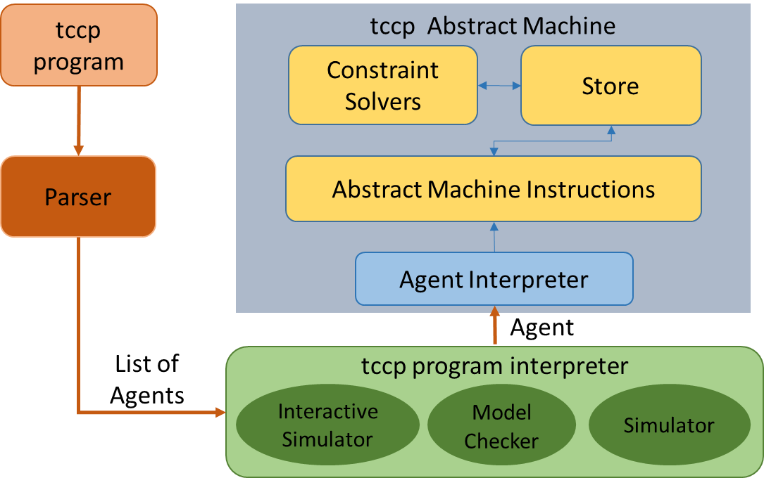
Figure 3: The architecture of the proposal

We now describe the main elements of this proposal in more detail: the store, the instructions of the abstract machine and the agent interpreter.

Subsection 3.1 Store

The store is the memory of the abstract machine, and is in charge of keeping the constraints over variables. The store is unique during the execution of tccp programs, which means that all agents access the same memory structure. In tccp, the preservation of the store consistency among all agents in execution is essential to guarantee the correct implementation of the parallel operator (rules par1 and par2 of fig:op_sem_tccp).

An agent of tccp is a light process with a short execution time. The natural mechanism of execution involves the creation of a large number of variables, with a restricted scope. We solve this issue by dividing the store into two memory elements: the symbol table and the global memory.

The symbol table is a tree structure used to determine the scope of a variable. Each tree node contains the local variables visible for a set of agents. There are two tccp agents that can define new variable scopes and, therefore, can add new nodes to the tree: exists and procedure call agents (rules hid and proc of fig:op_sem_tccp). The scope of the rest of the agents is associated with an already existing node. The global memory is responsible for keeping the constraints over the variables and provides the consistency of the store.

3.1.1 Abstract Machine Instructions

We now enumerate the set of basic instructions of the abstract machine used to implement the execution of agents. We need some preceding definitions. Let $x\in Var$, and $A$ be a tccp agent.

• $A.x$ denotes the variable named $x$ in the scope of $A$.

• $p.{x}$ represents the formal parameter ${x}$ of procedure $p$ in the tccp program.

In the description below, $global$ is the global store of the abstract machine (comprising the symbol table and the global memory), $A$ is the current agent to be executed by the machine, $c$ is a constraint, and $local_{1}$ and $local_{2}$ are the local stores produced by the parallel execution of agents.

The abstract machine provides the following basic functions:

• $is\_consistent():Boolean$: returns whether or not $global$ is consistent.

• $add\_variable(A.x)$: adds variables $x$ to $global$. Variables $x$ must be local to agent $A$.

• $add\_parameter(p.{x},{x^{\prime}})$: given a call $p({x^{\prime}})$ to a tccp procedure $p({x})$, adds new variables ${x}$ to $global$ and links it to the variables ${x^{\prime}}$ used in the procedure call.

• $add\_constraint(c)$: adds constraint $c$ to $global$.

• $entails(c):Boolean$: checks if $global$ entails constraint $c$.

• $merge(local_{1},local_{2})$: updates $global$ with the new constraints added to $local_{1}$ and $local_{2}$, if it is possible, that is, if no inconsistencies exist between the constraints in $local_{1}$ and $local_{2}$.

3.1.2 Agent Interpreter

The agent interpreter transforms each agent into the sequence of abstract machine instructions following the semantics given in fig:op_sem_tccp. fig:agentInterpreter depicts how the agent interpreter works. Given the current $A$, the interpreter first executes the corresponding abstract machine instructions, which directly interact with the store $global$, and then determines the agent $nA$ to be next executed.

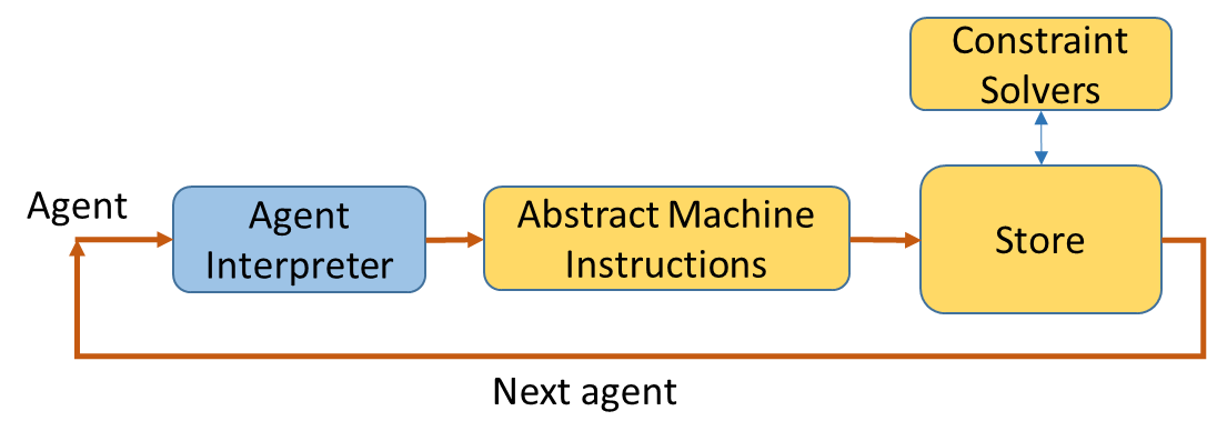
Figure 4: Interpreter of agents

In the following paragraphs, we define the execution of the current agent $A$, denoted as execute(A), inductively on the syntactic structure of $A$. We assume that the agent $A$ is executed on the global store $global$. Function $execute(A)$ returns the new store $local$ produced by the execution of agent $A$ and the set of agents to be next executed. Some agents, such as stop and tell, always return an empty set of agents.

parallel:

$A_{1}||A_{2}$

1. $is\_consistent()$: if it is true, continue to step 2 else stop

2. Let $execute(A_{1})=\langle local_{1},nA_{1}\rangle$

3. Let $execute(A_{2})=\langle local_{2},nA_{2}\rangle$

4. Return $\langle merge(local_{1},local_{2}),nA_{1}||nA_{2}\rangle$

tell(c)

1. $is\_consistent()$: if it is true, continue to step 2 else stop

2. $add\_constraint(c)$

3. Return $\langle global,\textsf{stop}\rangle$

choice:

$\sum_{i=1}^{n}\mathop{\mathsf{ask}}(c_{i})\rightarrow A_{i}$

1. $is\_consistent()$: if it is true, continue to step 2 else stop

2. If $\neg entails(c_{i})$ for $i=1,\dots,n$, proceed with step 4, else select randomly one branch $\mathop{\mathsf{ask}}(c_{i})\rightarrow A_{i}$ such that $entails(c_{i})$ holds and proceed with step 3

3. Return $\langle global,A_{i}\rangle$

4. Return $\langle global,\sum_{i=1}^{n}\mathop{\mathsf{ask}}(c_{i})\rightarrow A_{i}\rangle$

now:

$\mathop{\mathsf{now}}\>c\mathrel{\mathsf{then}}A\mathrel{\mathsf{else}}B$

1. $is\_consistent()$: if it is true, continue to step 2 else stop

2. if $entails(c)$ then return $execute(A)$, else return $execute(B)$

hiding:

$\mathop{\exists{x}}{}$

1. $is\_consistent()$: if it is true, continue to step 2, else stop

2. $add\_variable(A.x)$

3. Return $execute(A)$

procedure call:

$p({x}):-A$

1. $is\_consistent()$: if it is true, continue to step 2 else stop

2. $add\_parameter(p.{x},p.{x^{\prime}})$, where ${x^{\prime}}$ are the variable used in the procedure call $p({x^{\prime}})$

3. Return $\langle global,A\rangle$

Observe that the implementation of agents described above closely follows the agent semantics of fig:op_sem_tccp. Thus, proving the correctness of the implementation reduces to proving that the basic instructions of Section 3.1.1 update the store correctly.

Section 4 Implementation issues

We have implemented a tccp simulator based on the abstract machine presented in Section 3. The tool accepts tccp programs with linear constraints over arithmetic variables, and logic constraints over streams. A stream can store text or linear expressions over arithmetic variables.

The tccp machine has been implemented in Java. We have used existing third party Java libraries to implement the different elements of the simulation tool. The tccp machine includes two different constraint solvers, one for linear constraints and another for logic constraints. The first one is based on Parma Polyhedra Library [6] (PPL), a library that provides numerical abstractions such as convex polyhedra or grids. The constraint solver for linear constraints uses convex polyhedron to represent a system of linear constraints, and each dimension represents a variable. The polyhedron is universe (true) when all variables are unconstrained, and it is empty (false) when constraints are not satisfied. Moreover, PPL also provides methods to check if the polyhedron entails a specific constraint. The logic constraint solver has been developed from scratch, since it strongly depends on the memory model implemented. There are other Java constraint solvers, such as JaCoP [24], which supports a large variety of constraints (basic arithmetic operation constraints, logical and conditional constraints, regular constraints for the assignment to variables, etc.). This constraint solver is versatile and easy to use in solutions such as this proposal. However, we have preferred to use PPL, since we plan to extend our abstract machine and the simulation tool for modelling rectangular hybrid systems and PPL provides more suitable numeric abstraction to represent continuous variables and their evolution over time.

We have used ANTLR [21] to generate the parsers included in the simulator. Given a grammar described in the notation similar to BNF, ANTLR produces the base classes for the parser and visitor. We have extended the base visitor to control how to walk the parse-tree, and to specify the returned type. The tool includes a parser that transforms a tccp program from plain text into a list of Agent objects. In addition, there are independent parsers for linear constraints and logic constraints. They return respectively, PPL Constraint System and Stream objects.

Subsection 4.1 Store implementation

The store, presented in Section 3, has to keep and manage logic constraints over streams, and linear constraints over numeric variables, which are represented by convex polyhedron. To this end, the memory model is extended with a convex polyhedron, called $disc\_poly$, that saves linear constraints. Each dimension of $disc\_poly$ represents a variable. The dimension assigned will be the same until the end of the program execution. Consistently with the notion of store in tccp, polyhedron $disc\_poly$ is monotonic, that is, constraints are added but never removed.

The symbol table is a tree, whose nodes have an identifier and store the list of variables belonging to this scope. For each variable, the node keeps the symbol identifier and the memory position that saves its information. The need to use a tree instead of a list will be clear later, when we discuss the dynamic procedure generation.

The global memory is an array of registers, which keep the type of memory element, and a data field. Currently, there are four types of memory elements, and each type saves different information in the data field:

• Constant: the data field stores the value of the constant.

• Discrete variable: the data field stores the dimension that represents this variable in $disc\_poly$.

• Reference: the data field saves the referenced memory position.

• Functor: the element is a stream with head and tail. The data field keeps the memory position of the head. The tail is always stored in the next position from the head.

Below, we address the main issues of the store implementation, most of them are related to the characteristics of tccp enumerated in Section 3.

Store consistency

The store includes diverse structures that keep the different kinds of constraints and variables. The global consistency or inconsistency is determined as follows: the store is consistent if constraints over streams are consistent and $disc\_poly$ is not empty. In any other case, the store is inconsistent.

Dynamic procedure generation

Every procedure call adds a new node to the symbol table, and links it with its father node. The identifier of the new node will be propagated, if necessary, to the nodes of the agents in its scope. This new node contains the list of its parameters. If a parameter is associated with a variable or constant value, it points to the caller variable/constant position. If a parameter is associated with an arithmetic expression, the parameter is linked to a variable that is constrained by this expression. Observe that when more than one procedure calls are executed in parallel, the new nodes created have the same father node, and this is why the symbol table built is a tree.

Dynamic variable generation

The execution of an exists agent adds a new node in the symbol table that identifies the scope of the variables. The symbol table identifies and manages the potentially large number of variables with repeated names. Similarly to the dynamic procedure generation, the identifier of the exists node will be propagated, if necessary, to the nodes of the agents in its scope. When these agents are executed, they start looking for symbols in the node of its exists parent. If the symbol is not found, they look in the parent of the node, and repeat this process until they find the symbol or reach a node created by a procedure call.

Concurrency in the store

Agents executing in parallel have probably different views of the store, which can involve consistency problems. We address this issue by executing each agent with a copy of the memory structures that store the constraints. When concurrent agents have been executed, all the copies are merged in such a way that the resulting store is in the right state (consistent or not) and includes the right constraints. For instance, if $agent_{1}$ and $agent_{2}$ add constraints over arithmetic variables, each agent will modify a copy of $disc\_poly$, named $p_{1}$ and $p_{2}$, and after executing both agents $disc\_poly=p_{1}\cap p_{2}$.

Section 5 Evaluation

In this section, we evaluate the current simulator running the photocopier example, presented in sec:photocopier_example. This example has an infinite and non-deterministic behaviour. In the evaluation, we will execute a finite number of steps of the abstract machine. In addition, we need to repeat the same trace several times to obtain statistics. To this end, the user process always selects the last branch of the choice; that is, the user does not send commands to the photocopier.

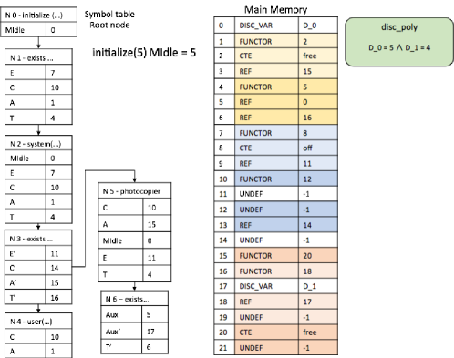
Figure 5: Photocopier example - store state 7 steps

We execute the example using the call initialize(MIdle) || tell(MIdle = 5). fig:copier_execution depicts the state of the store after carrying out 7 steps of the simulation. On the left hand side, we have the symbol table in which each node is created by a procedure call or an exists agent. The root node (N0) is created because the procedure call initialize(MIdle) that contains the parameter MIdle set to 5. In the next step, an exists agent is executed which creates the node N1 containing the list of local variables. Then, several tell agents and a procedure call to system are executed in parallel. The tell agents add values to the heads of A, T and E, and the procedure call adds a new node (N2) with the list of parameters of system pointing to the variables used in the call. In the following step, the exists agent is executed which creates a new node (N3), and the parallel agent comprising four tell agents, a procedure call to user and two ask agents. The first ask can proceed, but the second one blocks because A’ is unbound. Due to parallel execution of the procedure calls (user(C,A) $||$ photocopier(C,A’,MIdle,E’,T’)), nodes N3 and N4 are created. The rest of the nodes are generated in a similar way.

The main memory, on the right, holds information about the value of the variables during the execution. For example, positions 0 and 17 store the information of the variables of the system (MIdle, Aux and Aux’). Observe that Aux (position 5) is a reference to position 0, which keeps a variable represented in $disc\_poly$ by dimension 0. Another type of element in memory are functors, which represent stream variables. For example, position 1 is a functor whose head is a constant set to free, and whose tail is a reference to 15.

Table 1: Evaluation results

	30 steps	100 steps	500 steps
Symbol Table (nodes)	26	85	417
Global Memory (regiters)	78	239	1169
disc_poly (dimensions)	6	6	6
Heap used (MB)	4	4.1	7
Heap allocated (MB)	16.3	16.3	16.3
Parser (ms)	192	196	197
Simulation (ms)	87	192	2,170

tab:structures shows the size of the store with respect to the number of steps executed. In the example, an increment of steps implies that more procedure calls and exists agents are executed. Consequently, the number of nodes in the symbol table increases with the number of steps executed and similarly the size of the global memory. In addition, when a new element is added to a stream, three registers are allocated: the functor, the head and the tail. Observe that the photocopier example has linear constraints (Aux’ = Aux -1). Since the photocopier does not receive commands, the value stored in T is decremented until it is 0. In consequence, after some steps, $disc\_poly$ has 6 dimensions and the following constraint system:

$$D\_0=5\wedge D\_1=4\wedge D\_2=3\wedge D\_3=2\wedge D\_4=1\wedge D\_5=0$$

We have used the Java monitoring console to collect information regarding the execution time and the memory allocated. The tests have been carried out in a virtualized Ubuntu machine, with 2GB of RAM memory and one processor. The Java virtual machine is OpenJDK Client VM 24.95-b01. The bottom part of tab:structures also shows the average heap usage and execution times obtained by executing several times the same example. Observe that, the execution of the parser takes longer than executing 30 steps of the abstract machine. Obviously, when the number of steps is higher, the parser remains in the same magnitude, and the simulator consumes more time. The execution time has been measured without printing the symbol table and memory state, since printing slows down the execution. For example, the simulator execution time of 30 steps printing the status of symbol table each step takes an average of 187 ms, which is more or less the execution time of the parser. With respect to the memory, we have monitored the heap used and allocated. The memory used/allocated is not the real total memory used by the Java application. We should investigate how to obtain this information in future work.

Section 6 Related Work

In this section, we describe and compare other proposals in the literature for the implementation of concurrent, declarative or synchronous languages, some of which were mentioned in the Introduction.

Lustre [15] and SIGNAL [5, 11] share with tccp their declarative and synchronous character. Both languages are data-flow oriented, that is, programs operate over infinite sequence of values. They have been used for the modelling and analysis of industrial critical systems, which proves that synchronous languages are not only useful in academia. For example, Lustre is the language underpinning a wide range of tools [14], the most important being SCADE Suite [10], a toolset for modelling, simulating, verifying and generating certified code for critical systems. Similarly, POLYCHRONY [19] is the development framework of SIGNAL. It provides mechanisms for the design, simulation, verification and code generation for distributed hardware platforms.

Unlike our proposal, the final aim of the tools developed for Lustre and SIGNAL is to generate code, optimized for specific platforms. Instead, the main concern of our architecture is its compositional character and, in consequence, its ability to adapt to new constraint solvers, new language extensions, or new agent interpreters that execute the program differently. In fact, since the current implementation is based on an interpreted abstract machine running on Java, the performance completely depends on the underlying Java virtual machine.

In the context of concurrent logic programming, there are some older languages which share characteristics with tccp. For example, PARLOG [8] is a logic concurrent language descendent of PROLOG [18], intended to describe distributed systems. PARLOG supports fine-grain parallelism similar to that of tccp. Process communication is also carried out using streams, but it lacks global memory and mechanisms for hiding and creating new local variables. In contrast, PARLOG incorporates the notion of modes, associated with the process parameters, to synchronise them. In [13], the authors present an abstract machine for the implementation of PARLOG on uniprocessors. In this implementation, the PARLOG computation is represented by an AND/OR tree in which each node is a process that can be runnable or locked (waiting for some data), in a similar way to the tccp agents. Although, both proposals (tccp and PARLOG) agree that the agents (processes) have an associated sequence of instructions of the underlying abstract machine, the memory models are considerably different. This is principally because of the tccp hiding operator which makes it possible to define an arbitrary number of local variables. As regards implementation issues, both implementations provide simulators on the language, but use different target languages (C and Java).

Along the same lines, Kernel Language KL1 [27] is a committed-choice logic language based on the Guarded Horn Clauses GHC [28] intended to be target language for the implementation of concurrent logic languages. The main goal of KL1 is, therefore, the construction of efficient, production-quality programs to exploit physical parallelism. The implementation of KL1 was developed on the Parallel Inference Machine (PIM), which has a hierarchical memory-architecture where clusters have processing elements connected by a bus. In this implementation, the difficulties are also related to memory architecture and management.

With respect to tccp tools, [25] presents an interpreter of tccp implemented in Mozart-Oz [16]. The semantics of tccp is mapped into Mozart-Oz directly defining a translation from tccp to Mozart-Oz. Nevertheless, this work is not publicly available and does not included the latest features of tccp presented during the last years.

In [20], authors present a tccp interpreter, implemented in Maude. Similar to our proposal, they parse, interpret and simulate tccp programs. Their tool implements six Maude modules, one for each tccp entity (agents, constraints, programs, store, constraint system and operational semantics) which are used to directly translate from tccp to Maude.

Section 7 Conclusions and Future Work

We have presented an abstract machine for tccp, which defines the behaviour of tccp agents over a memory architecture called store. The abstract machine is composed of different modules which have been design to be as independent as possible. Most of the architecture components are unaware of the actual implementation of the memory or the particular implementation of the agent behaviour. We think that this approach facilitates and simplifies the development of tools for tccp. In addition, we have implemented a tool for the simulation of tccp following this abstract machine architecture. The tool has been implemented in Java, and uses other external libraries and frameworks to implement different elements. For example, we use ANTLR to generate the parsers, and PPL to implement the constraint solver for linear constraints.

We have evaluated the simulator with the photocopier example, running different number of abstract machine steps. We have presented the state of the abstract machine store after executing the example, and shown some performance measures obtained with profiling tools. We believe that the performance is acceptable, although we should improve the memory model to achieve more efficient implementations for constructing, for instance, a tccp model checker.

Although, the current tool at http://morse.uma.es/tools/tccp may be only used to simulate some available tccp codes, we plan to extend its capability by allowing users to simulate their own programs. In fact, the tool only lacks a frontend that manages syntax errors. In addition, due to the different implementation approaches followed by tool [20] and ours, it is difficult to compare performance of both tools but we plan to do it in the near future.

As future work, we wish to extend the abstract machine to hy-tccp [2]. hy-tccp is an extension of tccp for hybrid systems, which adds a notion of continuous time and new agents to describe the continuous dynamics of hybrid systems. hy-tccp is independent from the kind of constraints over continuous variables. To implement a hy-tccp simulator, we will assume that the hybrid systems are rectangular. Because of the independence amongst the different entities which compose implementation, the extension of the current abstract machine will involve adding the new agents of the hy-tccp language and probably new abstract machine instructions. In addition, the parser should be extended to recognise the new agents. Finally, we will reuse PPL as the constraint solver for constraints over continuous variables.

References

- [1]
- [2] D. Adalid, M. Gallardo & L. Titolo (2015): Modeling Hybrid Systems in the Concurrent Constraint Paradigm. Electronic Proceedings in Theoretical Computer Science 173, 10.4204/EPTCS.173.1.
- [3] H. Aït-Kaci (1991): Warren’s Abstract Machine: A Tutorial Reconstruction. MIT Press, Cambridge, MA, USA.
- [4] M. Alpuente, M. del Mar Gallardo, E. Pimentel & A. Villanueva (2005): Quantitative Aspects of Programming Languages (QAPL 2004) A semantic framework for the abstract model checking of tccp programs. Theoretical Computer Science 346(1), pp. 58 – 95, 10.1016/j.tcs.2005.08.009.
- [5] P. Amagbégnon, L. Besnard & P. Le Guernic (1995): Implementation of the Data-flow Synchronous Language SIGNAL. In: Proceedings of the ACM SIGPLAN 1995 Conference on Programming Language Design and Implementation, PLDI ’95, ACM, New York, NY, USA, pp. 163–173, 10.1145/207110.207134.
- [6] R. Bagnara, P.M. Hill, E. Ricci & E. Zaffanella (2005): Special Issue on the Static Analysis Symposium 2003 Precise widening operators for convex polyhedra. Science of Computer Programming 58(1), pp. 28 – 56, 10.1016/j.scico.2005.02.003.
- [7] F. de Boer, M. Gabbrielli & M. Meo (2000): A Timed Concurrent Constraint Language. Information and Computation 161(1), pp. 45 – 83, 10.1006/inco.1999.2879.
- [8] K. Clark & S. Gregory (1986): PARLOG: Parallel Programming in Logic. ACM Trans. Program. Lang. Syst. 8(1), pp. 1–49, 10.1145/5001.5390.
- [9] M. Comini, L. Titolo & A. Villanueva (2011): Abstract diagnosis for timed concurrent constraint programs. TPLP 11(4-5), pp. 487–502, 10.1017/S1471068411000135.
- [10] Esterel Technologies (2016): SCADE Suite. Available at http://www.esterel-technologies.com/products/scade-suite/.
- [11] A. Gamatié & T. Gautier (2010): The Signal Synchronous Multiclock Approach to the Design of Distributed Embedded Systems. IEEE Transactions on Parallel and Distributed Systems 21(5), pp. 641–657, 10.1109/TPDS.2009.125.
- [12] T. Gautier & P. Le Guernic (1987): SIGNAL: A declarative language for synchronous programming of real-time systems. In G. Kahn, editor: FPCA, Lecture Notes in Computer Science 274, Springer, pp. 257–277, 10.1007/3-540-18317-5_15.
- [13] S. Gregory, I.T. Foster, A.D. Burt & G.A. Ringwood (1989): An abstract machine for the implementation of PARLOG on uniprocessors. New Generation Computing 6(4), pp. 389–420, 10.1007/BF03037448.
- [14] N. Halbwachs (2005): A synchronous language at work: the story of Lustre. In: Proceedings. Second ACM and IEEE International Conference on Formal Methods and Models for Co-Design, 2005. MEMOCODE ’05., pp. 3–11, 10.1109/MEMCOD.2005.1487884.
- [15] N. Halbwachs, P. Caspi, P. Raymond & D. Pilaud (1991): The synchronous data flow programming language LUSTRE. Proceedings of the IEEE 79(9), pp. 1305–1320, 10.1109/5.97300.
- [16] S. Haridi, P. Van Roy, P. Brand & C. Schulte (1998): Programming languages for distributed applications. New Generation Computing 16(3), pp. 223–261, 10.1007/BF03037481.
- [17] E.Y. Kang, G. Perrouin & P.Y. Schobbens (2013): Model-Based Verification of Energy-Aware Real-Time Automotive Systems. In: Engineering of Complex Computer Systems (ICECCS), 2013 18th International Conference on, pp. 135–144, 10.1109/ICECCS.2013.27.
- [18] R.A. Kowalski (1988): The Early Years of Logic Programming. Commun. ACM 31(1), pp. 38–43, 10.1145/35043.35046.
- [19] P. Le Guernic, J.-P. Talpin & J.-C. Le Lann (2003): POLYCHRONY for System Design. Journal of Circuits, Systems and Computers 12(03), pp. 261–303, 10.1142/S0218126603000763.
- [20] A. Lescaylle & A. Villanueva (2009): The tccp Interpreter. Electronic Notes in Theoretical Computer Science 258(1), pp. 63 – 77, 10.1016/j.entcs.2009.12.005.
- [21] T. Parr (2013): The Definitive ANTLR 4 Reference, 2nd edition. Pragmatic Bookshelf.
- [22] J. Qian, J. Liu, X. Chen & J. Sun (2015): Modeling and Verification of Zone Controller: The SCADE Experience in China’s Railway Systems. In: Complex Faults and Failures in Large Software Systems (COUFLESS), 2015 IEEE/ACM 1st International Workshop on, pp. 48–54, 10.1109/COUFLESS.2015.15.
- [23] V.A. Saraswat & M. Rinard (1990): Concurrent Constraint Programming. In: Proceedings of the 17th ACM SIGPLAN-SIGACT Symposium on Principles of Programming Languages, POPL ’90, ACM, New York, NY, USA, pp. 232–245, 10.1145/96709.96733.
- [24] J. Sedlacek & T. Hurka (2016): JaCoP - Java Constraint Programming solver. Available at http://jacop.osolpro.com/.
- [25] T. Sjöland, E. Klintskog & S. Haridi (2001): An interpreter for Timed Concurrent Constraints in Mozart (Extended Abstract).
- [26] L.A. Tuan, M.C. Zheng & Q.T. Tho (2010): Modeling and Verification of Safety Critical Systems: A Case Study on Pacemaker. In: Secure Software Integration and Reliability Improvement (SSIRI), 2010 Fourth International Conference on, pp. 23–32, 10.1109/SSIRI.2010.28.
- [27] K. Ueda & T. Chikayama (1990): Design of the Kernel Language for the Parallel Inference Machine. The Computer Journal 33(6), pp. 494–500, 10.1093/comjnl/33.6.494.
- [28] K. Ueda (1986): Logic Programming ’85: Proceedings of the 4th Conference Tokyo, Japan, July 1–3, 1985, chapter Guarded horn clauses, pp. 168–179. Springer Berlin Heidelberg, Berlin, Heidelberg, 10.1007/3-540-16479-0_17.